Understanding Global Systems Today—A Calibration of the World3-03 Model between 1995 and 2012

Abstract

In 1972 the Limits to Growth report was published. It used the World3 model to better understand the dynamics of global systems and their relationship to finite resource availability, land use, and persistent pollution accumulation. The trends of resource depletion and degradation of physical systems which were identified by Limits to Growth have continued. Although World3 forecast scenarios are based on key measures and assumptions that cannot be easily assessed using available data (i.e., non-renewable resources, persistent pollution), the dynamics of growth components of the model can be compared with publicly available global data trends. Based on Scenario 2 of the Limits to Growth study, we present a calibration of the updated World3-03 model using historical data from 1995 to 2012 to better understand the dynamics of today’s economic and resource system. Given that accurate data on physical limits does not currently exist, the dynamics of overshoot to global limits are not assessed. In this paper we offer a new interpretation of the parametrisation of World3-03 using these data to explore how its assumptions on global dynamics, environmental footprints and responses have changed over the past 40 years. The results show that human society has invested more to abate persistent pollution, to increase food productivity and have a more productive service sector.

1. Introduction

One use of system dynamics models is to analyse real systems in order to understand and improve some undesirable performance patterns [1]. Models are also applied to policy testing [2], exploring what-if scenarios [3], or policy optimization [4]. Within a finite planet, material consumption and the degradation of physical systems cannot grow forever. Since economic growth is coupled with real growth in consumption, overshoot and collapse of the global system is expected to occur in the future. If measures are taken to decouple economic growth from real material consumption growth then it is still possible to avoid these limits. This is the main message of the Limits to Growth (LTG) work [5]. Commissioned by the Club of Rome in the early 1970s, the LTG based its results and analysis on the World3 model first published in 1972.

Despite authors’ effort to communicate the results of the model simulations in a clear and accessible way [5,6,7,8], misunderstandings and lively debates took place within the research community [9,10]. An assessment of the LTG scenarios 36 years after the original publication [9,11] showed that the trends of historical data compared favourably with key features of the 1972’s “standard run scenario”. The “standard run” has a global collapse in the economy and population around the middle of this century.

Although the powerful message conveyed by the “standard run” overshoot and collapse scenario shaped the media debate for the last 40 years, in the LTG the assumptions on natural resources availability were deemed conservative. The LTG policy recommendations were set on the basis of Scenario 2 that, differently from the “standard run” scenario, accounted for enough resource availability to sustain economic growth for a longer time. In this case the overshoot and collapse of economic and population dynamics was due to the unsustainable accumulation of persistent pollution in the environment linked to resource use. Randers [12] argued that “It now appears that the tightest constraint on physical growth is not resource scarcity, or vulgar shortage of raw materials. Rather the most pressing limit seems to be on the emission side. To be concrete, the world appears to have much more fossil fuels than was assumed, indeed more than man can burn without causing serious climate change”.

While World3 was not intended to produce point forecasts of the future but to explore behavioural modes, new data can be used to recalibrate the relationships associated with the behaviour of the system. Moreover, the relation between data and the model structure, and its eventual influence on the recalibration, can be assessed. In light of new data relating to the global system, the LTG authors refined World3 twice, resulting in new versions named World3-91 and World3-03 [7,8]. These updates were concerned with numerical values of parameters and relations rather than structural modifications of the model, and helped to validate the model outcomes against real data. Recent work aimed at simplifying the model to help with communication of results also led to greater insight into global dynamics and the issues raised by LTG [13,14].

In this paper we present a re-run and recalibration of the World3-03 model using historical data from 1995 to 2012. The resulting parameters (i.e., the outcomes of the calibration) and their variation from the parameters in World3-03, are assumed to provide insight on the current status of the global system, as well as highlighting open issues linked to the model structure and how they may affect the representativeness and meaningfulness of LTG today. The recalibration exercise has several advantages. In particular, it allows us to (i) better understand the origin of World3-03 behavioural modes and how the structure affects the model’s results; and (ii) support the development of global modelling today by pointing out how those original assumptions around behaviour modes have changed with time.

Given the difficulty in estimating the World3 measures of non-renewable resources and persistent pollution variables (given the uncertainty of non-renewable resources reserves, and different data quality and availability for persistent pollution impacts by sector at the global level), and given the uncertainty of assessing the cost in terms of economic output as well as the positive effect in coping with resource constraints of adaptive technology, this paper does not attempt to provide forecasts further than the year 2012. Therefore, we do not run the model forward in time and cannot explore the overshoot and collapse behaviours. The paper is limited to a static representation of the dynamic behaviour mode of the global system using time series from 1995 to 2012. The available historical data used are: (i) industrial output; (ii) service output; (iii) population; (iv) birth rate; (v) life expectancy; (vi) arable land.

Section 2 of the paper reviews the original World3 model and outcomes highlighting the key sources of uncertainty within the model in terms of structural assumptions and forecasts for the future. Section 3 describes the methodology used to analyse and calibrate World3-03, explaining how we limited the modifications in the model structure which are needed to match the available data with model behaviours. Section 4 presents the calibration itself and the results of our analysis, discussing the role of the variation of single parameters on the structure and functioning of the world system of today. Section 5 provides conclusions based on our findings, limitations to this work, next steps and suggestions for future research.

2. The Limits to Growth World3 Model Review

2.1. System Dynamics as a Modelling Paradigm

System dynamics (SD) is a mathematical modelling paradigm first developed by Forrester [2] to study complex systems. It is grounded on the concepts of stocks, flows, information flows, feedback loops and delays. Every stock is a numerical variable which determines the status of the system. It represents an accumulation whose variation is determined by the difference between its inflows and outflows. Information flows connect stock variables with inflows and outflows within the system. Stocks, flows, and information flows together determine the structure and the interconnectivity within the model.

Within the network of model relations, every path that links a variable to its inflow is called a feedback loop, which is the first important tool to describe and understand system complexity using SD. Feedback loops may be positive/reinforcing loops (when a feedback loop tends to increase the value of a variable), or negative/balancing loops (when a feedback loop tends to reduce the value of a variable or to stabilise it on a given value). Feedback loops are the basic component in SD because they are able to capture the complexity of the system by showing the causal relations between the model components.

The second important SD tool is the presence of delays. Within a system, a delay represents the natural time for a set of actions or policies in the system to be effective and measurable. They can be either “information” or “material” delays [15]. Information delays are concerned with the time required by social beings to adapt to environmental changes (e.g., time needed by households to perceive natural resource scarcity or the threat of climate change). Material delays describe material in transit within the system (e.g., time for investments to materialize into the increased productivity of plants). Given the role of information and material delays, the consequences of initial behaviours may not be immediately visible but affect the system over time.

2.2. World3—Purpose and Structure

Commissioned by the Club of Rome in 1970s, World3 was built at a time when industrial capital accumulation was considered the driving factor of economic and population growth. The model builds on several assumption on the structure of the economy and the evolution of the society which are linked to the scientific knowledge and historical period in which the model was developed. However, such assumptions are demonstrated to be still true, and the model can be modified to reflect numerical changes revealed over time by means of minor changes to the coefficients and relations [7,8]. In World3, by using material resources, industrial capital is increased to provide material equipment and increase the land available for both services and agricultural activities in order to provide satisfactory health services and nutrition to the population. The representation of exponential population growth is assured by recorded continuous increases in life expectancy and by increasing birth rates. Industrial capital is assumed to grow exponentially as well, thus supporting agricultural processes, and generating local pollution, lands erosion, and maintaining high levels of land fertility through production activities. Industrial and agricultural processes generate persistent pollutants that accumulate in the environment and tend to decrease land fertility and impact people’s life expectancy. It is worth noting that in the 70s the service and telecommunication sectors were not highly developed, and renewable resources were not sufficiently deployed to be a credible substitute to fossil fuels. Economic growth is modelled as mainly consisting of material growth, where every unit of capital and person is responsible for one fraction of material depletion, land erosion and pollutants generation (both local and persistent).

World3 is a system dynamics simulation model used to develop alternative global scenarios by describing the most likely behaviour mode which emerges from the interconnectivity of economic growth and Earth system limits. The planetary boundaries are represented by (i) non-renewable resources; (ii) persistent pollution and (iii) land availability and fertility. Economic growth is represented by the linkage between (iv) population and (v) industrial capital. World3 is based on Forrester’s global model World2 [16]. As World2 was mainly built on the intuition of its developer, World3 aimed at filling the gap between World2 and the literature available up to 1972. This makes World3 larger in size and more grounded in theory. However, they still share very similar basic assumptions on planetary limits and on the core components of the global system. World3 and World2 simulate the dynamic behaviour of the global system from the year 1900 to 2100.

While other more complex models have been developed over the past few decades, including integrated assessment models [17,18], World3 offers a simpler construct to understand the overall dynamics and behaviours of the global system. The simplicity and transparency of World3 should allow policy makers and modellers to better understand and engage with those global trends, behaviour modes and risks.

In Table 1 the key model variables (stocks) in World3 are presented and their main inflows and outflows identified. For example, the stock variable Arable Land represents all the land available for Food production. Its inflow is represented by the Land Development Rate, which is dependent on food demand. The outflow is represented by (i) Land Removal For Urban and Industrial Use, which is dependent on Population increases; and (ii) Arable Land Erosion Rate, which is proportional to Food production through the variable Land Yield. This means that Arable Land may increase its potential in food production through higher Land Yield, but it could also decrease its potential in food production if it is allocated to urban or industrial use (residential or factory buildings), or affected by the negative effects of soil erosion on land productivity.

Table 1. Stocks and flows within the World3 model.

Stocks	Inflows	Outflows
Population 0 to 14: All living people younger than 15 years old	Births: Variable fraction of Population 15 to 44. Dependent on Human Fertility.	Maturation 14 to 15: Constant fraction of Population 0 to 14 Deaths 0 to 14: Variable fraction of Population 0 to 14. Dependent on Life expectancy.
Population 15 to 44: All living people between 15 and 44 years old	Maturation 14 to 15: Constant fraction of Population 0 to 14.	Maturation 44 to 45: Constant fraction of Population 15 to 44. Deaths 15 to 44: Variable fraction of Population 15 to 44. Dependent on Life expectancy.
Population 45 to 64: All living people between 45 and 64 years old	Maturation 44 to 45: Constant fraction of Population 15 to 44.	Maturation 64 to 65: Constant fraction of Population 45 to 64. Deaths 45 to 64: Variable fraction of Population 45 to 64. Dependent on Life expectancy.
Population 65 Plus: All living people older than 64 years old	Maturation 64 to 65: Constant fraction of Population 45 to 64.	Deaths 65 Plus: Variable fraction of Population 65 Plus. Dependent on Life expectancy.
Potentially Arable Land: Measured in hectares, it imposes the maximum limit of land of the planet. It is assumed to be converted to Arable Land at cost which rises with land depletion.	-	Land Development Rate: Dependent on Food demand. The aim is to add have Arable Land to sustain Food production through the variable Land Yield.
Arable Land: Measured in hectares, it represents the all land under cultivation, and represents the basis for food production.	Land Development Rate: Dependent on Food demand. The aim is to have Arable Land to sustain Food production through the variable Land Yield.	Land Removal For Urban and Industrial Use: Dependent on Population increases. Arable Land Erosion Rate: Proportional to Food production through the variable Land Yield.
Urban And Industrial Land: Land converted in Urban and Industrial Areas.	Land Removal For Urban and Industrial Use: Dependent on Population increases.	-
Land Fertility: Determines how much food a hectare of land can produce. When pollution rises it can decrease to zero, but can also regenerate.	Land Fertility Regeneration: Variable fraction of Industrial Agricultural Inputs.	Land Fertility Degradation: Proportional to the amount of Persistent Pollution.
Non-Renewable Resources: All the materials of the planet used in Industrial Processes.	-	Resource Usage Rate: Variable in proportion of Industrial Output.
Persistent Pollution: Every pollutant from industrial and agricultural activity which accumulates in the environment and is harmful for both Land Fertility and People Life Expectancy.	Persistent Pollution Appearance Rate: Variable in proportion to Industrial Output and Agricultural Inputs Arable Land (summed up).	Persistent Pollution Assimilation Rate: Variable, decreases if Persistent Pollution increases.
Industrial Capital: Material capital which composes all Industrial Processes which extract materials and sustain the global economy by material injection.	Industrial Capital Investment: Variable fraction of Industrial Output.	Industrial Capital Depreciation: Constant fraction of Industrial Capital.
Service Capital: Material capital which produced output from intangibles.	Service Capital Investment: Variable fraction of Industrial Output.	Service Capital Depreciation: Constant fraction of Service Capital.
Agricultural Inputs: Material capital used for agricultural activity.	Variable fraction of Industrial Output.	Constant fraction of Agricultural Inputs.

Table 1. Stocks and flows within the World3 model.

Stocks	Inflows	Outflows
Population 0 to 14: All living people younger than 15 years old	Births: Variable fraction of Population 15 to 44. Dependent on Human Fertility.	Maturation 14 to 15: Constant fraction of Population 0 to 14 Deaths 0 to 14: Variable fraction of Population 0 to 14. Dependent on Life expectancy.
Population 15 to 44: All living people between 15 and 44 years old	Maturation 14 to 15: Constant fraction of Population 0 to 14.	Maturation 44 to 45: Constant fraction of Population 15 to 44. Deaths 15 to 44: Variable fraction of Population 15 to 44. Dependent on Life expectancy.
Population 45 to 64: All living people between 45 and 64 years old	Maturation 44 to 45: Constant fraction of Population 15 to 44.	Maturation 64 to 65: Constant fraction of Population 45 to 64. Deaths 45 to 64: Variable fraction of Population 45 to 64. Dependent on Life expectancy.
Population 65 Plus: All living people older than 64 years old	Maturation 64 to 65: Constant fraction of Population 45 to 64.	Deaths 65 Plus: Variable fraction of Population 65 Plus. Dependent on Life expectancy.
Potentially Arable Land: Measured in hectares, it imposes the maximum limit of land of the planet. It is assumed to be converted to Arable Land at cost which rises with land depletion.	-	Land Development Rate: Dependent on Food demand. The aim is to add have Arable Land to sustain Food production through the variable Land Yield.
Arable Land: Measured in hectares, it represents the all land under cultivation, and represents the basis for food production.	Land Development Rate: Dependent on Food demand. The aim is to have Arable Land to sustain Food production through the variable Land Yield.	Land Removal For Urban and Industrial Use: Dependent on Population increases. Arable Land Erosion Rate: Proportional to Food production through the variable Land Yield.
Urban And Industrial Land: Land converted in Urban and Industrial Areas.	Land Removal For Urban and Industrial Use: Dependent on Population increases.	-
Land Fertility: Determines how much food a hectare of land can produce. When pollution rises it can decrease to zero, but can also regenerate.	Land Fertility Regeneration: Variable fraction of Industrial Agricultural Inputs.	Land Fertility Degradation: Proportional to the amount of Persistent Pollution.
Non-Renewable Resources: All the materials of the planet used in Industrial Processes.	-	Resource Usage Rate: Variable in proportion of Industrial Output.
Persistent Pollution: Every pollutant from industrial and agricultural activity which accumulates in the environment and is harmful for both Land Fertility and People Life Expectancy.	Persistent Pollution Appearance Rate: Variable in proportion to Industrial Output and Agricultural Inputs Arable Land (summed up).	Persistent Pollution Assimilation Rate: Variable, decreases if Persistent Pollution increases.
Industrial Capital: Material capital which composes all Industrial Processes which extract materials and sustain the global economy by material injection.	Industrial Capital Investment: Variable fraction of Industrial Output.	Industrial Capital Depreciation: Constant fraction of Industrial Capital.
Service Capital: Material capital which produced output from intangibles.	Service Capital Investment: Variable fraction of Industrial Output.	Service Capital Depreciation: Constant fraction of Service Capital.
Agricultural Inputs: Material capital used for agricultural activity.	Variable fraction of Industrial Output.	Constant fraction of Agricultural Inputs.

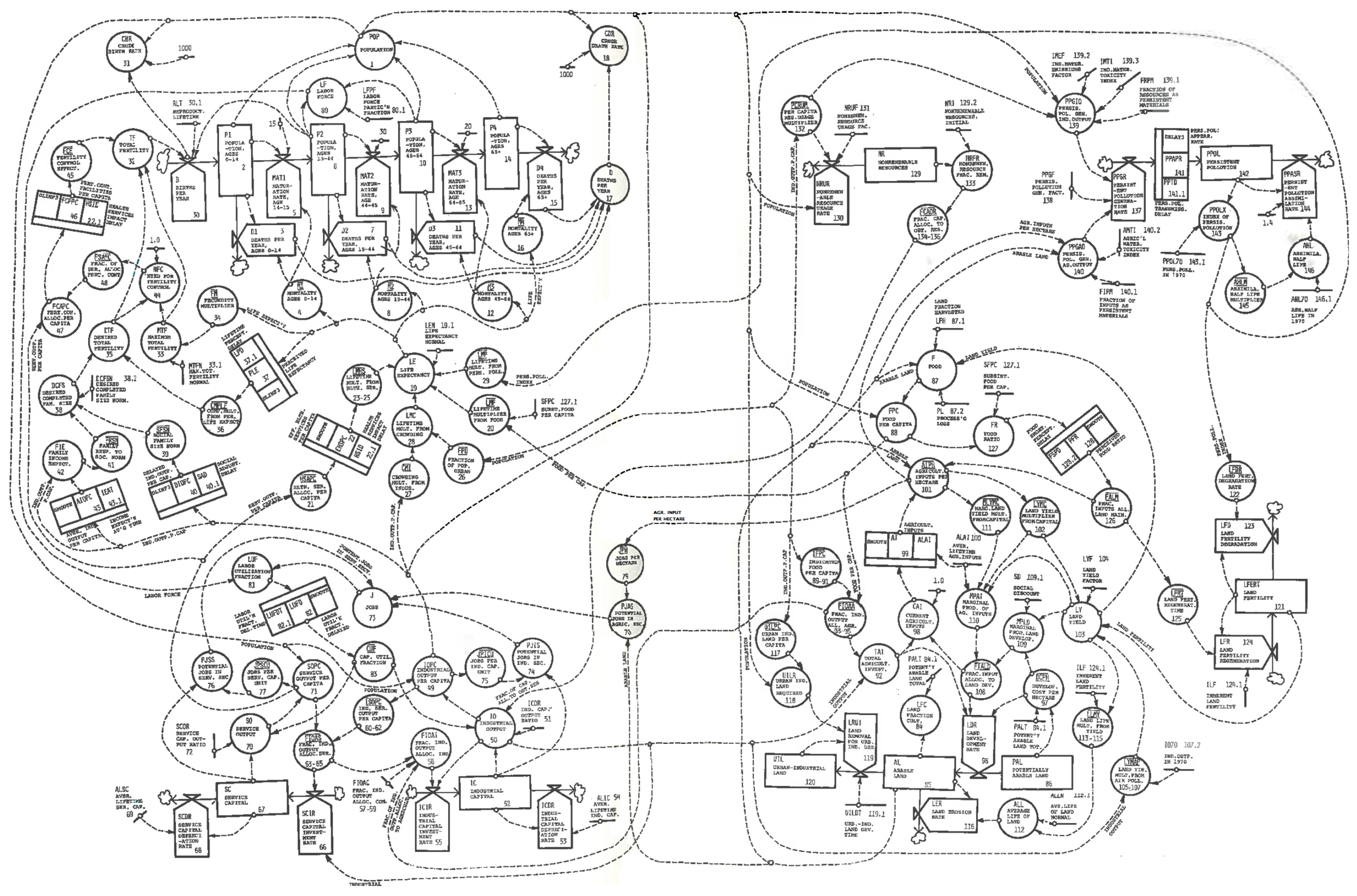
Figure 1 shows the stock and flow diagram of World3 as first published in 1972. The stock and flow structure represents the pillars of the model and are all mutually interconnected. The network of relationships is assumed to capture the complexity of the world we live in within a model useful to study the dynamics of real capital growth under the constraints of a finite planet.

The eight World3 variables presented in the LTG as the main scenario outputs are (i) Total Population, (ii) Birth Rate; (iii) Death rate; (iv) Industrial Output Per Capita; (v) Service Output Per Capita; (vi) Food Per Capita; (vii) Non-Renewable Resources; and (viii) Persistent Pollution Index. Due to the unavailability of data (Meadows indicated that only 0.1% of data were available to build World3 model [19]), only (i), (ii), (iii) were defined consistently with data publicly available. However, assumptions were made for the others.

Figure 1. Stock and flow diagram (dynamo representation) of World3 model structure [6].

Figure 1. Stock and flow diagram (dynamo representation) of World3 model structure [6].

2.3. World3 Limits

Forecasting the future is not easy, and every forecast is based on assumptions which reflect the knowledge available at the time in which it is made and the interpretation that the modeller places on that knowledge. Modelled in System Dynamics, World3 was designed to generate patterns for possible uncertain future scenarios of the global system. The main assumption of the LTG in building the scenarios is that investing in technology, which supports economic growth, is the way to overcome physical constraints in the system. The cost of technology deployment, within LTG, is considered a reduction of industrial output which is proportional to the burden of the problem to be solved. For example, the higher the emissions rate in the environment, the higher the cost to control their damaging effects. While the standard run of World3 assumes no adaptive technology investment and economic collapse due to resource scarcity, the Scenario 2 of LTG assumes a much higher level of non-renewables available alongside more efficient use of those.

On the basis of Scenario 2, assumptions in developing and deploying adaptive technology to cope with planetary limits are made, and run through four separate scenarios (Scenario 3 to 6 in [8]). Three important structures able to capture the complexity of this process are endogenously represented in the model—(i) the effect of technology in containing persistent pollution; (ii) the effect of technology in increasing land yield and reducing land erosion; and (iii) the effect of technology in reducing non-renewable resources consumption. Their effect is seen in the proportional reduction of economic output and in the dynamic change of three important parameters which quantify the effects of economic output on planetary limits. These parameters could be varied to control and even nullify the effect of physical constraints (Table 2).

Table 2. World3 parameters which quantify natural constraints to economic growth.

Parameter	Value in Standard Run [Range]	Controlled Flow	Meaning and Use of the Parameter
Resource Use Factor 1	1 [0–1]	Resource Usage	Resource use variation determines the rate of depletion of Non-Renewable Resources. Setting it to zero correspond to null resource depletion, which means infinite Non-Renewable Resources.
Land Yield Factor 1	1 [1–not limited] plus shift between table functions which indicate two different uses of lands and relative impact on Arable Land Erosion Rate.	Arable Land Erosion	Its increases determine how much Food can be produced using one hectare of land in addition to conventional land yield from capital. However, the greater the Land Yield per hectare, the higher the Arable Land Erosion Rate.
Persistent Pollution Generation Factor 1	1 [0–1]	Persistent Pollution Appearance Rate	Its variation determines the amount of Persistent Pollution generated from the combined effects of Agricultural and Industrial activities. Setting it to zero assumes null Persistent Pollution generation.

Table 2. World3 parameters which quantify natural constraints to economic growth.

Parameter	Value in Standard Run [Range]	Controlled Flow	Meaning and Use of the Parameter
Resource Use Factor 1	1 [0–1]	Resource Usage	Resource use variation determines the rate of depletion of Non-Renewable Resources. Setting it to zero correspond to null resource depletion, which means infinite Non-Renewable Resources.
Land Yield Factor 1	1 [1–not limited] plus shift between table functions which indicate two different uses of lands and relative impact on Arable Land Erosion Rate.	Arable Land Erosion	Its increases determine how much Food can be produced using one hectare of land in addition to conventional land yield from capital. However, the greater the Land Yield per hectare, the higher the Arable Land Erosion Rate.
Persistent Pollution Generation Factor 1	1 [0–1]	Persistent Pollution Appearance Rate	Its variation determines the amount of Persistent Pollution generated from the combined effects of Agricultural and Industrial activities. Setting it to zero assumes null Persistent Pollution generation.

3. Methodology of Analysis

Extensive sensitivity analysis and tests have been performed on World3 since 1972 [6,19,20]. However, there is no standardized way to test the results of a model [1,15,21]. Criticism of World3 included the relationship between material growth (Industrial Output) and intangible assets growth (Service Output) assumed to produce economic output without consuming resources. According to this structure, Industrial Output can stabilize before Population, which implicitly assumes the behaviour of the global population leads to a decoupling of its material consumption [22]. This assumption is difficult to prove at the aggregate level of World3. Furthermore, the structure of innovation and technology dimensions applied to the system are very intuitive and not based on robust statistical evidence [6].

Model calibration, “the process of estimating the model parameters to obtain a match between observed and simulated structures and behaviours” [23], can be considered the ultimate test of a model. In the LTG, the match between every simulation run and the historical data from the year 1900 to the year 1970 is considered a test of the model itself. In addition, a continuous review process has been undertaken by the LTG team [7,8]. Therefore, we believe that running an updated version of World3 (World3-03) based on data which are consistent, comparable and updated could contribute to improve the understanding of how the dynamics of growth matches real data.

World3 was designed to explore general future behavioural trends rather than provide data robust forecasts. As the world has not already experienced an overshoot and collapse we cannot recalibrate the physical limits within World3. Therefore, this paper does not look into the future and is intended to be a static representation of reality. We use a calibration to provide a match between the system behaviour generated by World3-03 and recent data. By using the selected data trends as constraints to control the model behaviour, and allowing the input parameters to vary, we argue that the resulting parameter values, in comparison with the ones used to generate the base run scenario, carry enough information to inform consistent conclusions regarding the status of the global system.

3.1. Model Calibration as Descriptive Methodology

In this paper we assume that, by generally capturing the dynamics of the global system, there is a combination of parameters which allows the behaviour of World3 outcomes to perfectly match with real data. The methodology adopted is to make sure that the combination of parameters is also meaningful and provides consistent conclusions.

The original scenarios in World3 included a set of policy responses, starting in selected years, which introduced non-linear trends in growth. These years changed in the further versions of World3 (policies starting in 1975, 1995, 2002). The policies relate to rates of accumulation of knowledge and technology and, with a certain delay, to deployment of such technology. These non-linear effects are extremely useful when looking in the long term forecast of the state of the world. However, as we are more interested in providing a snapshot in time to define the current dynamics of the global system rather than characterise long term trends or explore the overshoot scenarios these policy response scenarios can be just approximated by single parameters.

For our purposes, we do not need long time series from where non-linear effects of economic growth would emerge. We start the simulation from the year 1995, and include 18 years of time series to identify the current trend of the most important variables. The selection of parameters to be considered, and the groups of parameters calibrated at any step during the calibration helps us to develop a description of the global system as it is today according to the World3 structural assumptions. We rely on the emergent property of the calibration to generate the parameters, which, in comparison with the base run scenario proposed in the LTG, helps describing the state of the world today. The following steps were performed:

(1)

The World3-03 structure is taken on the basis of previous studies.

(2)

The addition of a few parameters, mainly to allow scaling of real data into World3 values, was necessary. However, no structural assumptions have been challenged or changed from the original version of World3-03.

(3)

Screening of all edited parameters and selection of a sub-group of them to present in this paper was necessary to add meaning to the output of the calibration process.

3.2. Historical Data Used and Changes in World3-03

Lyneis and Pugh [24] consider the calibration an iterative process done “by hand”. The first aspect we considered to ensure a good calibration was to use enough historical data to cover the behaviour modes of every stock variable in the model. Then, the parameters chosen to run the calibration have to be dependent on the constraints imposed by the historical data. In other words, historical data represents pathways through which World3 outputs based on model behaviours should pass, and model behaviours can vary only in function of the values of the parameters. Allowing a selected parameter to vary within a range of values gives a degree of freedom to the model behaviour to find a way to match with historical data. An iterative process to vary the values of parameters (or groups of parameters) within certain ranges was performed to find the correct set of inputs which matched most closely with the historical data pathways.

A preliminary comparison of the metadata of World3 variable definitions was used to identify real data time series to use (Table 3).

Table 3. Match between historical data and World3-03 stock variables.

World3 Variable	Dataset Variable	Reference Dataset	Stock Variables Covered
Population	Population, total	United Nations Population division	Population 0 to 14
			Population 15 to 44
			Population 45 to 64
			Population 65 plus
Birth Rate	Birth rate, crude (per 1000 persons)	United Nations Population division	Population 0 o 14
			Population 15 to 44
			Industrial Capital
			Service Capital
Life Expectancy	Life expectancy at birth, total (years)	United Nations Population division	Population stocks
			Arable Land
			Service Capital
Industrial Output	Industry value added 2005 constant	World Bank National account Data	Industrial Capital
			Population 0 to 14
			Arable Land
Service Output	Service value added 2005 constant	World Bank National account Data	Service Capital
			Population stocks
Arable Land	Arable Land (hectares)	Food and Agriculture Organization (FAO) data	Arable Land
			Potentially Arable Land
			Urban and Industrial Land

Table 3. Match between historical data and World3-03 stock variables.

World3 Variable	Dataset Variable	Reference Dataset	Stock Variables Covered
Population	Population, total	United Nations Population division	Population 0 to 14
			Population 15 to 44
			Population 45 to 64
			Population 65 plus
Birth Rate	Birth rate, crude (per 1000 persons)	United Nations Population division	Population 0 o 14
			Population 15 to 44
			Industrial Capital
			Service Capital
Life Expectancy	Life expectancy at birth, total (years)	United Nations Population division	Population stocks
			Arable Land
			Service Capital
Industrial Output	Industry value added 2005 constant	World Bank National account Data	Industrial Capital
			Population 0 to 14
			Arable Land
Service Output	Service value added 2005 constant	World Bank National account Data	Service Capital
			Population stocks
Arable Land	Arable Land (hectares)	Food and Agriculture Organization (FAO) data	Arable Land
			Potentially Arable Land
			Urban and Industrial Land

Where data does not match, perfectly simple scaling parameters were adopted such as the inflation rate between 1968 dollars (as used in World3) and 2005 dollars (as reported by the World Bank). Table 4 summarizes these scaling parameters, resulting in our version, called the World3-03-Edited version, used in this study.

Table 4. Parameters and variable additions to World3-03-Edited structure.

Additional Elements in the Model Structure	Role of Parameter
Parameter Lifetime Multiplier From Services	Controls the effect of Service Output on Health Services
Parameter Investment in Services	Controls the fraction of Industrial Output allocated to Service capital
Parameter W3-Reality Exchange Rate	Exchange rate which allows a comparison with World3 capital measures with 2005 dollar values
Auxiliary variable Industrial Output 2005 Value	Allows a comparison between current World Bank data and World3 Industrial Output
Auxiliary variable Service Output 2005 Value	Allows a comparison between current World Bank data and World3 Service Output
Auxiliary variable Arable Land Harvested	Used to compare FAO’s data with World3 Arable Land
Parameter Arable Land Erosion Factor	Used as indicator for current use of lands in relation to Arable Land Erosion Rate

Table 4. Parameters and variable additions to World3-03-Edited structure.

Additional Elements in the Model Structure	Role of Parameter
Parameter Lifetime Multiplier From Services	Controls the effect of Service Output on Health Services
Parameter Investment in Services	Controls the fraction of Industrial Output allocated to Service capital
Parameter W3-Reality Exchange Rate	Exchange rate which allows a comparison with World3 capital measures with 2005 dollar values
Auxiliary variable Industrial Output 2005 Value	Allows a comparison between current World Bank data and World3 Industrial Output
Auxiliary variable Service Output 2005 Value	Allows a comparison between current World Bank data and World3 Service Output
Auxiliary variable Arable Land Harvested	Used to compare FAO’s data with World3 Arable Land
Parameter Arable Land Erosion Factor	Used as indicator for current use of lands in relation to Arable Land Erosion Rate

3.2.1. Demographic-Social Related Variables

Correspondence in the values of Population, Birth Rate, and Life Expectancy perfectly match between public dataset definitions and World3 variables definitions [6]. For clarity they were all taken from United Nations Population Division. Total Population is the aggregated value of all the populations of any country estimated at midyear. Birth Rate indicates the number of live births per year every 1000 persons. Life expectancy at birth indicates the number of years offspring infant would live if prevailing patterns of mortality at the time of its birth were to stay the same throughout its life. In World3, Population is governed by the dynamics of mortality (directly related with Life Expectancy) and Births (directly related with Total Fertility). In Life Expectancy four different factors converge, e.g., (i) health services; (ii) crowding effect; (iii) food per capita; and (iv) persistent pollution. Total Fertility is calculated using a more complex structure which derives from the dynamics of Industrial Output Per Capita and Service Output per Capita.

3.2.2. Economic Related Variables

In World3, Service Output and Industrial Output are generated by a multiplication between respective “Capital” stock variables and “Capital-Output Ratio” parameters. The metadata definition for those stock variables are as follows [6]:

• “Service capital in the model is associated with the activities listed under ISIC (International Standard Industrial Classification) divisions 6 through 9: Wholesale and retail trade, restaurants and hotels; transport, storage, and communication; financing, insurance, real estate, and business services; and community, social, and personal services.”
• “Industrial capital stock provides the output in ISIC divisions 2 through 5: Mining and quarrying, manufacturing; electricity, gas, and water; and construction.”

Nowadays, the closest available data which we used for our comparison is:

(1)

Service, etc., value added (constant 2005 US Dollars) from the aggregation World Bank National Account’s national level data. “...this includes ISIC divisions 50–99 which are value added in wholesale and trade (including hotels and restaurants), transport, and government, financial, professional, and personal services such as education, health care, and real estate services. Also included are imputed bank service charges, import duties, and any statistical discrepancies noted by national compilers as well as discrepancies arising from rescaling.”

(2)

Industry, value added (constant 2005 US dollars) obtained by aggregating national level World Bank National Account Data. “…this includes ISIC divisions 10–45, which comprises value added in mining, manufacturing, construction, electricity, water, and gas.”

Every capital unit in World3 is a material unit rather than a monetary unit. To allow a comparison between our data and World3 ones, we extended the model structure with one additional parameter and two variables. The parameter is W3-Reality Exchange Rate. Its role is to convert the value of the variables Industrial Output and Service Output into 2005-dollars. The resulting values are recorded in the new variables Industrial Output 2005 value and Service Output 2005 value, which in turn are used for the comparison with the historical data.

In World3, the Service Output is calculated from Service Capital by dividing it by the parameter Service Capital Output Ratio. In turn, Service Capital is accumulated through allocations (investment) from Industrial Output and depleted by Service Capital Depreciation. The main effect of Service Output in World3 is in the development of Health Services calculated as fraction of the former. Heath Services represent the facilities necessary to sustain Life Expectancy and to allow Population growth control. By performing preliminary calibration analysis it was clear that a sufficient degree of freedom (available parameters to vary) was not present to allow the model behaviour to converge to the historical data. Thus, two other variables have been created to allow a correct match. The first is Investments in Services which is linked to the model as a correction factor between Industrial Output and investments in Service Capital. The variable is assumed to be higher than 1 and applied as a multiplication in the relationship. The second variable is Lifetime Multiplier from Services which corrects the relationship between Service Output and Health Services. These additions allowed the correct match between the historical values of Service Output, Industrial Output and Life Expectancy.

3.2.3. Agricultural-Land-Related Variables

In World3, the variable Arable Land is defined as “all areas which are used from time to time or full-time to grow crops and includes area under annual crops, area under permanent crops (tree crops, banana, sugar cane), area under temporary grass and fodder crops, and fallow” [6]. The FAO’s definition of Arable Land considers “land under temporary meadows for mowing or for pasture, land under market or kitchen gardens, and land temporary fallow. However, land abandoned as a result of shifting cultivation is excluded”. The differences in the two metadata requires the addition of the new variable Arable Land Harvested which is derived from the multiplication of the stock Arable Land and the already existing parameter Land Fraction Harvested. The Land Fraction Harvested parameter is considered to be 70%. The added variable Arable Land Harvested is used for the comparison in the calibration.

Arable Land is the basic quantity which, together with Industrial Output and Land Fertility, determines the level of Food production. Food production is required to sustain human Life Expectancy. However, according to the structure of World3-03, Land Fertility dynamics are dependent exclusively on the level of Persistent Pollution dynamics.

The main constraint of the Land sector in relation to World3 dynamics is represented by the combination of the Potentially Arable Land initial value (which represents the maximum total availability of land in the planet) and the dynamics of Arable Land Erosion Rate, which represents a permanent outflow of land from the system. The Arable Land Erosion Rate is assumed to increase at high levels of land exploitation (see Figure 2). The standard run scenario of World3-03 uses the curve Land Life Multiplier from Land Yield (LLMFLY) Table 1 (red curve in Figure 2) to define this erosion rate. The numerical function of this increase is set out in a pre-defined table within World3 (the table functions). However, technology to support the better use of Arable Land allows a gradual change from LLMFLY Table 1 to LLMFLY Table 2 (red curve to green curve in Figure 2). LLMFLY Table 2 is assumed to have a lower impact in eroding land than LLMFLY Table 1. For the purpose of our study, we add the new parameter Arable Land Erosion Factor which allows us to vary the impact of erosion between the two curves so as to better fit real data. Its range of variation is constrained between 0 and 1. The 0 value corresponds to using the Table 1, the 1 value corresponds to the Table 2, and every value in between correspond to any of the curves shown in Figure 2.

Figure 2. Variation of the parameter Arable Land Erosion Factor between the two table functions used to define the impact of increases in Land Yield to Arable Land Erosion.

Figure 2. Variation of the parameter Arable Land Erosion Factor between the two table functions used to define the impact of increases in Land Yield to Arable Land Erosion.

4. Calibration

4.1. Initialization of the Calibration Process and Calibration Parameters Selection

The first step of the initialization of the calibration is to link together selected historical data and correspondent World3-03-Edited variables (shown in Table 3). Secondly, the 1995 values (initial values) of four stock variables (i.e., every population cohort is analysed and updated based on the data of the United Nations Population Division Report [25]) and one parameter which are covered by historical data have been updated. The updated parameter is Processing Loss, which is meant to take into account of percentage of food which is produced by Arable Land but is wasted in the food supply chain, plus a small percentage which considers area that is cultivated for purpose different from food production (for example, cotton). 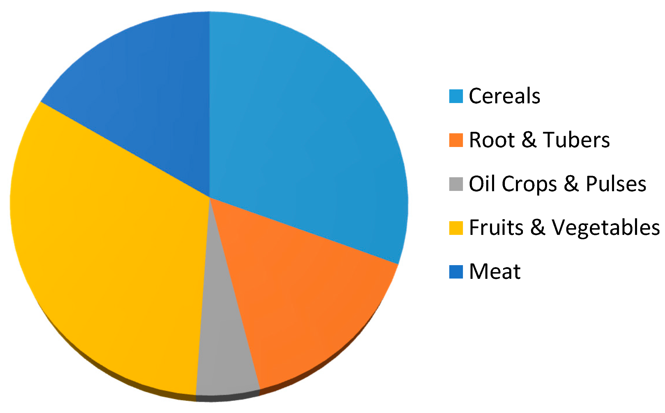Food wasted after its production has been approximated globally [26] for (i) cereals; (ii) root and tubers; (iii) oil crops and pulses; (iv) fruits and vegetables; and (v) meat. In order to convert those data into a single global loss figure, the meat production value had to be multiplied by 7 to account for its larger land footprint per unit of weight and then summed up to the other four categories. Figure 3 shows the relative waste from each type of food category. The resulting aggregate Processing Loss is 32%. We increase it by a small percentage to also take into account land cultivated for other purposes and estimate global Processing Loss to be 35%. This is comparable to the value of 10% considered in the World3 base run scenario.

Figure 3. The relative food processing loss (waste) from different food categories globally. The total food processing loss is estimated to be 35% of food production.

Figure 3. The relative food processing loss (waste) from different food categories globally. The total food processing loss is estimated to be 35% of food production.

Thirdly, the model structures surrounding Persistent Pollution and Non-Renewable Resources stock variables were initially omitted from the study. Since there is no accurate way to measure real quantities which are comparable with those variables (global physical limits or absolute level of recoverable resources), these structures were nullified for the initial part of the calibration, to be re-included once all other parameters are able to represent the dynamics of growth for the World3 model. By re-including these parameters post initial calibration we can test the robustness of our model. It is worth noting that their effects have a limited contribution on the model behaviour in the time frame considered (1995–2012).

The modification within the initial calibration of the model follows:

• Resources Usage Factor 1 parameter, which quantifies the amount of resources extracted from the stock Non-Renewable Resources is set to 0. Setting it to 0 corresponds to considering infinite resources. Non-renewable resources demand is always satisfied to allow economic growth.
• Persistent Pollution Generator Factor1 parameter, which determines the rate of pollution generated by the aggregated effects of Industrial and Agricultural activities is set to 0. Setting this parameter to 0 eliminates pollution generation and in turn its harmful effects on Population and Land Fertility.
• Initial Persistent Pollution parameter, which determines the level of Persistent Pollution at the beginning of the simulation, is set to 0.
• Initial Land Fertility parameter, which determines the level of Land Fertility at the beginning of the simulation, is set to 600. Together with the exclusion of persistent pollution effect, Land Fertility is reduced to be a simple constant for the time frame of the entire simulation.

The final step in the initialization is to perform a sensitivity analysis to screen every parameter of World-03-Edited in order to select the smallest number of parameters whose variations affects the behaviour of the model outcomes in relation to the constraints imposed by the selected historical data. The remaining parameters that do not affect the outcomes are assumed to have the values in the World3-03 initial structure.

For the purpose of this study, sensitivity screening of every parameter of World3-03-Edited consisted of performing several calibrations to (i) build confidence in the model behaviour and (ii) identify every parameter whose variation does not affect the result of the calibration. The total number of resulting parameters in the model is 59. By eliminating the effects of Non-Renewable Resources and Persistent Pollution, this number was reduced to 44 parameters. By manually updating the initial values of the population cohort stocks and the value of the parameter Processing Loss, the number of parameters subjected to this analysis was reduced to 39. A second outcome of this activity was the identification of the values of the new parameters W3-Reality Exchange Rate and Land Fraction Harvested that converge to fixed values. W3-Reality Exchange Rate converts 2005 dollars into 1968 dollars and we calculate a conversion factor is $7.19 for every World3-03 dollar. This compares favourably with the actual inflation figure for the United States over this period ($5.61) but it is not possible to externally validate the global figure as global inflation data does not exist for this whole period. Given inflation is likely to have been higher in emerging and developing countries, we feel this figure can be justified. Land Fraction Harvested converged to the value 0.68 (in the standard scenario mode it was 0.7).

The sensitivity screening analysis allowed the selection of a group of 16 parameters (Table 5) that are used for the next phase of the calibration. The remaining were assumed to have the value imposed in the standard run scenario of World3-03. According to the role every parameter had in the model behaviour, the final group was split into three sub-groups. For the purpose of this study these sub-groups were named (i) “Economic” related parameters, concerned with the behaviours constrained between Industrial Output, Service Output and Life Expectancy variables; (ii) “Agricultural-Food” related parameters that mainly affects the linkages constrained within Arable Land, Industrial Output and Life Expectancy variables; and (iii) “Demographic-Social” related parameters which concerned the model behaviours constrained by Services Output, Industrial Output, Life Expectancy and Birth Rate variables.

Table 5. List of the 15 parameters used in the calibration and sub-group division according to their role in the model.

Parameter	Parameter Role in World3-03-Edited Model	Sub-group
Initial Industrial Capital	Initial value of Industrial Capital stock variable	Economic
Initial Service Capital	Initial value of Service Capital stock variable	Economic
Industrial Capital Output Ratio 1	Represents the ratio which defines the amount of output produced by every unit of Industrial Capital	Economic
Service Capital Output Ratio 1	Represents the ratio which defines the amount of output produced by every unit of Service Capital	Economic
Average Life of Service Capital 1	Represents the average amount of years the Service Capital can be used before depreciating	Economic
Investment in Services (*)	Acts as corrective factor in the allocation of investments form Industrial Output to Service Capital	Economic
Initial Arable Land	Initial value of Arable Land stock variable	Agriculture-Food
Initial Potentially Arable Land	Initial value of Potentially Arable Land stock variable	Agriculture-Food
Land Yield Factor 1	Determines the contribution of technology improvements in the food production in addition to conventional agricultural systems	Agriculture-Food
Arable Land Erosion Factor (*)	Determines how land are carefully used in relation to the level of exploitation in the food production	Agriculture-Food
Desired completed family size normal	Describes the desired family size by the average family	Demographic-Social
Lifetime Multiplier from Services (*)	A correction factor which defines the effect of Service Output on Health services	Demographic-Social
Income expectation averaging time	Average time spent from people to change their desires in family planning according to economic wages	Demographic-Social
Health services impact delay	Determines the delay between the changes in service output per capita and the time in which health facilities (hospital, doctors) are operative	Demographic-Social
Social adjustment delay	Determines the time population need to change their family planning to adapt to demographic changes	Demographic-Social
Lifetime perception delay	Determines the time spent by people to adapt to changes in relation to their expectation of life	Demographic-Social

* parameters that have been added to World3-03 structure for the purpose of this study (see Table 4).

Table 5. List of the 15 parameters used in the calibration and sub-group division according to their role in the model.

Parameter	Parameter Role in World3-03-Edited Model	Sub-group
Initial Industrial Capital	Initial value of Industrial Capital stock variable	Economic
Initial Service Capital	Initial value of Service Capital stock variable	Economic
Industrial Capital Output Ratio 1	Represents the ratio which defines the amount of output produced by every unit of Industrial Capital	Economic
Service Capital Output Ratio 1	Represents the ratio which defines the amount of output produced by every unit of Service Capital	Economic
Average Life of Service Capital 1	Represents the average amount of years the Service Capital can be used before depreciating	Economic
Investment in Services (*)	Acts as corrective factor in the allocation of investments form Industrial Output to Service Capital	Economic
Initial Arable Land	Initial value of Arable Land stock variable	Agriculture-Food
Initial Potentially Arable Land	Initial value of Potentially Arable Land stock variable	Agriculture-Food
Land Yield Factor 1	Determines the contribution of technology improvements in the food production in addition to conventional agricultural systems	Agriculture-Food
Arable Land Erosion Factor (*)	Determines how land are carefully used in relation to the level of exploitation in the food production	Agriculture-Food
Desired completed family size normal	Describes the desired family size by the average family	Demographic-Social
Lifetime Multiplier from Services (*)	A correction factor which defines the effect of Service Output on Health services	Demographic-Social
Income expectation averaging time	Average time spent from people to change their desires in family planning according to economic wages	Demographic-Social
Health services impact delay	Determines the delay between the changes in service output per capita and the time in which health facilities (hospital, doctors) are operative	Demographic-Social
Social adjustment delay	Determines the time population need to change their family planning to adapt to demographic changes	Demographic-Social
Lifetime perception delay	Determines the time spent by people to adapt to changes in relation to their expectation of life	Demographic-Social

* parameters that have been added to World3-03 structure for the purpose of this study (see Table 4).

4.2. Calibration with and without Environmental Limits

By iterating the process of calibrating each group of parameters separately, it is possible to obtain a meaningful convergence between model behaviour modes and the selected historical data. By calibrating the model without environmental limitations, the methodology produces a set of parameters which show clear patterns in comparison to the initial study.

World3-03 assumes that the cost of technology is determined by the implemented level of technology rather than the available level of technology [8]. In World3-03, the initial time to start accumulating knowledge for developing technology solutions is 2002 with a 20-year delay to implement such technology [8]. Therefore, each adaptive effect would not have any impact during the whole time frame considered within this study, and to include effects of environmental limits in the model over the timescale considered, it is sufficient to manually include the effects of the structures of non-renewable resources and Persistent Pollution in the following way:

• Resources Usage Factor parameter, which quantifies the amount of resources extracted from the stock Non-Renewable Resources is set to 1. Setting it to 1 corresponds to assuming resource consumption compatible with the Scenario 2 trends.
• Persistent Pollution Generator Factor 1 parameter, which determines the rate of pollution generated by the aggregated effects of Industrial and Agricultural activities is set to 1. Setting this parameter to 1 assumes pollution generation and in turn its harmful effect to Population and Land Fertility at the same level as Scenario 2.
• Initial Persistent Pollution parameter, which determines the level of Persistent Pollution at the beginning of the simulation, is set to the same value obtained from running Scenario 2 until the year 1995.
• Initial Land Fertility parameter, which determines the level of Land Fertility at the beginning of the simulation, is set to the same value obtained from running Scenario2 until the year 1995, i.e., 563 vegetable equivalent kilograms of food per hectare per year.

By iterating the process with the same 16 parameters group by group, we obtain a new convergence between historical data and model behaviour. Any difference in the calibration values obtained using these two approaches—with and without environmental limits—allows us to check on the robustness of our assessment of World3 dynamics.

4.3. Calibration Results

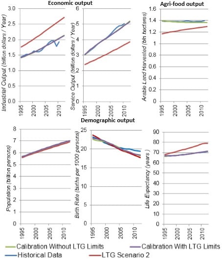
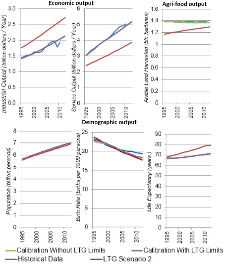
The conclusions drawn from the calibration are limited to the assumptions of Limits to Growth. In order to perform a consistent analysis, the parameters values as well as the relative model behaviour outcomes are presented in contrast to the Scenario 2 parameter values and behaviour modes of World3-03.

4.3.1. Economic Parameters and Outputs

In this category we include parameters and outputs which are related to Industrial Output, Service Output, and their mutual interdependence. Table 6 summarises the calibrated values compared to Scenario 2.

Table 6. Result of the calibration process in relation and parameter variation in comparison with World3-03 Scenario 2.

Parameter	Value Scenario 2	Value Calibration Without Limits	Value Calibration With Limits	Variation meaning
Industrial Capital-Output Ratio 1	3	3.64	3.64	There are lower rates of Industrial Output from every unit of Industrial Capital compared to the Scenario 2 of World3. This is due to more investment in technology to decouple industrial growth from planetary impacts.
Service Capital-Output Ratio 1	1	0.579	0.577	The productivity of Service Output per unit of Service Capital is higher than in the Scenario 2.
Investment in Services (*)	1 (not relevant)	2.07	2.02	There are higher investments in Service Capital than in the Scenario 2.
Average Life of Service Capital 1	20	24.07	24.02	Service Capital have longer life than in the Scenario 2

* parameters that have been added to World3-03 structure for the purpose of this study (see Table 4).

Table 6. Result of the calibration process in relation and parameter variation in comparison with World3-03 Scenario 2.

Parameter	Value Scenario 2	Value Calibration Without Limits	Value Calibration With Limits	Variation meaning
Industrial Capital-Output Ratio 1	3	3.64	3.64	There are lower rates of Industrial Output from every unit of Industrial Capital compared to the Scenario 2 of World3. This is due to more investment in technology to decouple industrial growth from planetary impacts.
Service Capital-Output Ratio 1	1	0.579	0.577	The productivity of Service Output per unit of Service Capital is higher than in the Scenario 2.
Investment in Services (*)	1 (not relevant)	2.07	2.02	There are higher investments in Service Capital than in the Scenario 2.
Average Life of Service Capital 1	20	24.07	24.02	Service Capital have longer life than in the Scenario 2

* parameters that have been added to World3-03 structure for the purpose of this study (see Table 4).

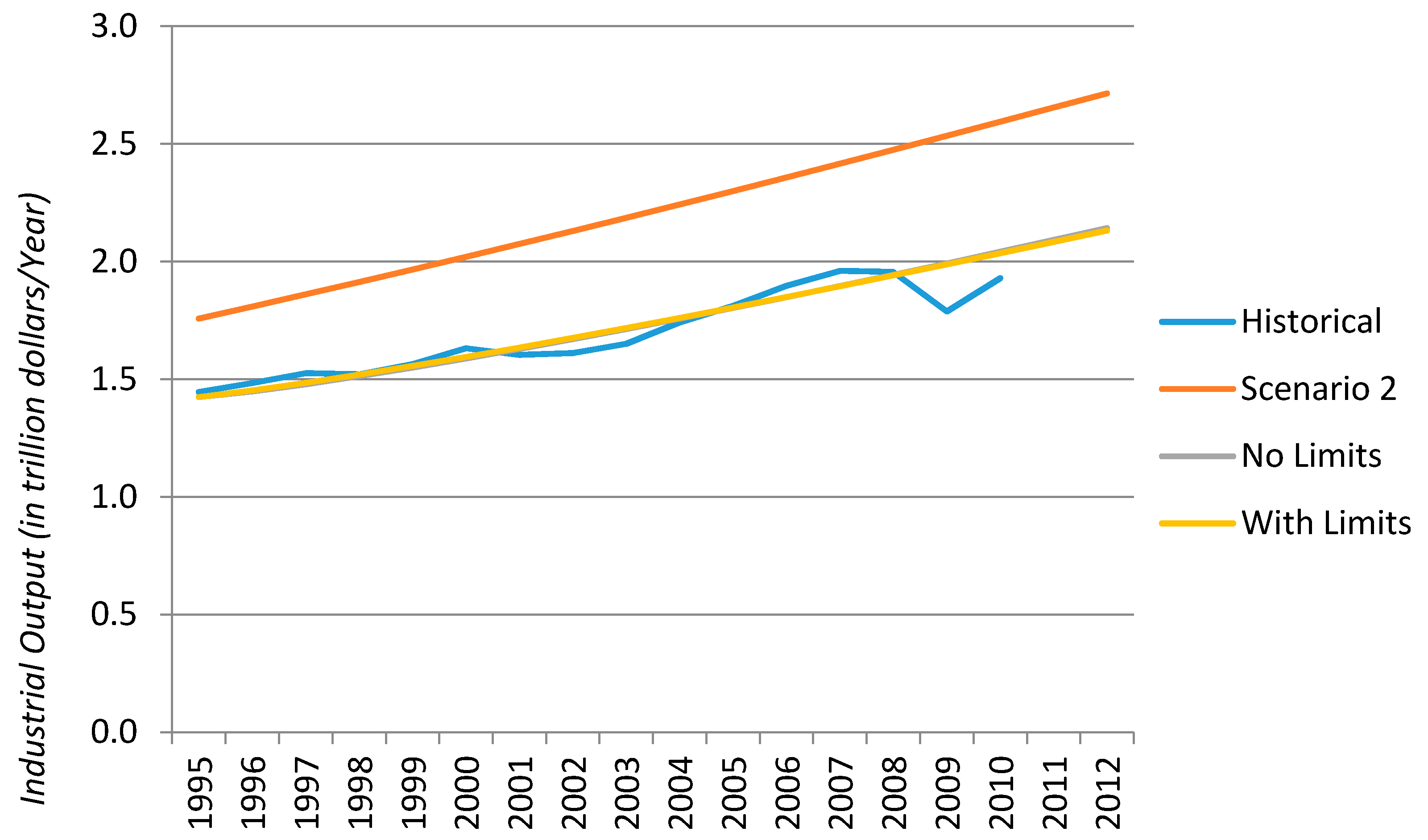
Starting with the parameter Industrial Capital-Output Ratio 1 we find a positive variation in comparison with the Scenario 2 in both the calibration with and without limits. This represents a decrease in the added value per unit of Industrial Capital. In World3 every technology improvement policy modelled in the agriculture, persistent pollution and non-renewable resources sectors are assumed to directly drive increases in the Industrial Capital-Output Ratio. The resulting value obtained can be interpreted as the current global system having developed more efficient technologies than expected which benefit planetary limits (Figure 4). We have invested more in technologies to decouple growth from planetary impacts than anticipated in Scenario 2 of World3.

Figure 4. Industrial output comparison between historic (real) data, Scenario 2 of World3 and the calibrated World3. Values in 1968 trillion dollars.

Figure 4. Industrial output comparison between historic (real) data, Scenario 2 of World3 and the calibrated World3. Values in 1968 trillion dollars.

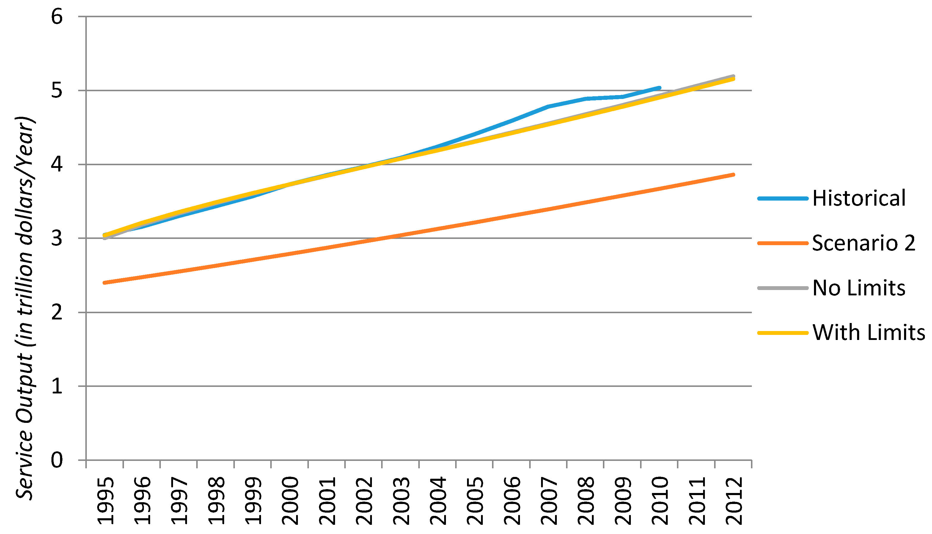
According to the variation of the parameter Investment in Services, the outflows from Industrial Output to Service Capital are underestimated in World3-03 model (about half that in the real data). In addition to this, the calibrated value of Service Capital-Output Ratio increases the effect of this underestimation. Every unit of Service Capital is over 70% more productive than in Scenario 2. In addition it seems that the average life of capital is higher in the calibration runs. Industrial Output is following a slower growth trend than Scenario 2, whereas Service Output follows a much higher trend as well as growing at higher increasing rate than estimated in Scenario 2 (Figure 5).

Figure 5. Service Output comparison between historic (real) data, Scenario 2 of World3 and the calibrated World3. Values in 1968 trillion dollars.

Figure 5. Service Output comparison between historic (real) data, Scenario 2 of World3 and the calibrated World3. Values in 1968 trillion dollars.

4.3.2. Agricultural-Food-Related Parameters and Outputs

This category concerns the dynamics of Arable Land and the parameters representing how much food is produced with the current level of Arable Land (Land Yield Factor 1) and how this production affects the erosion of arable land (Arable Land Erosion Factor).

The main values obtained (Table 7) suggest that significant improvements in food production and techniques to manage land erosion are in place compared to Scenario 2 of World3. Land Yield increases higher than 60% are seen and agricultural practices are much closer (Arable Land Erosion Factor higher than 90%) to the positive rather than the negative extreme represented by curves Land Life Multiplier From Land Yield Table 1 and Table 2 (see Figure 2).

It is worth noting that, by forcing the parameter Processing Loss to be 35% [26] rather than 10% as in the Scenario 2, the resulting effect of the model calibration is to increase the other parameter which directly affects the Food production through improved Land Yield (Land Yield Factor 1 is assumed to convey the effect of technology for increased productivity of land), and increase the level of Arable Land (the increase of Arable Land Erosion Factor reduces the erosion of Arable Land), which in turn affects Life Expectancy, which has been used as constraint variable for the calibration. Even though these parameters may indicate an increased productivity of land as well as better practices in managing land, this effect may be caused by a different interpretation of how food waste is accounted for to determine the parameter Processing Loss in comparison to LTG.

Table 7. Result of the calibration process in relation and parameter variation in comparison with World3-03 Scenario 2.

Parameter	Value Scenario 2	Value Calibration Without Limits	Value Calibration With Limits	Variation Meaning
Land Yield Factor 1	1	1.634	1.672	There is a higher contribution from technology improvement resulting in higher food production from the same amount of available Arable Land
Arable Land Erosion Factor (*)	0	0.92	0.94	The Arable Land erosion factor more closely follows the good practice outlined within LTG
Initial Land Fertility	600 (1900 value)	600 (1995 value)	563 (1995 value)	Land Fertility is assumed to be lower when Persistent pollution is activated

* parameters that have been added to World3-03 structure for the purpose of this study (see Table 4).

Table 7. Result of the calibration process in relation and parameter variation in comparison with World3-03 Scenario 2.

Parameter	Value Scenario 2	Value Calibration Without Limits	Value Calibration With Limits	Variation Meaning
Land Yield Factor 1	1	1.634	1.672	There is a higher contribution from technology improvement resulting in higher food production from the same amount of available Arable Land
Arable Land Erosion Factor (*)	0	0.92	0.94	The Arable Land erosion factor more closely follows the good practice outlined within LTG
Initial Land Fertility	600 (1900 value)	600 (1995 value)	563 (1995 value)	Land Fertility is assumed to be lower when Persistent pollution is activated

* parameters that have been added to World3-03 structure for the purpose of this study (see Table 4).

As Figure 6 shows, Arable Land historical data is constant over time. The Arable Land dynamic described in the model shows a continuous land development process that substitutes for what is eroded or allocated to urban and industrial uses. In the future, if population and food consumption patterns continue to grow, Arable Land would first consume the whole Potentially Arable Land and then erosion would gradually start a slow decrease below current levels resulting in lower output levels in the food chain [27]. The inclusion of the dynamic behaviour of Land Fertility, driven by changes in Persistent Pollution, has an effect of reducing arable land erosion, and for the time considered in this study, it results in a slightly better fit with historical data.

Figure 6. Arable Land comparison between historic (real) data, Scenario 2 of World3 and the calibrated World3. Measured in billion hectares.

Figure 6. Arable Land comparison between historic (real) data, Scenario 2 of World3 and the calibrated World3. Measured in billion hectares.

4.3.3. Demographic-Social Parameters and Outputs

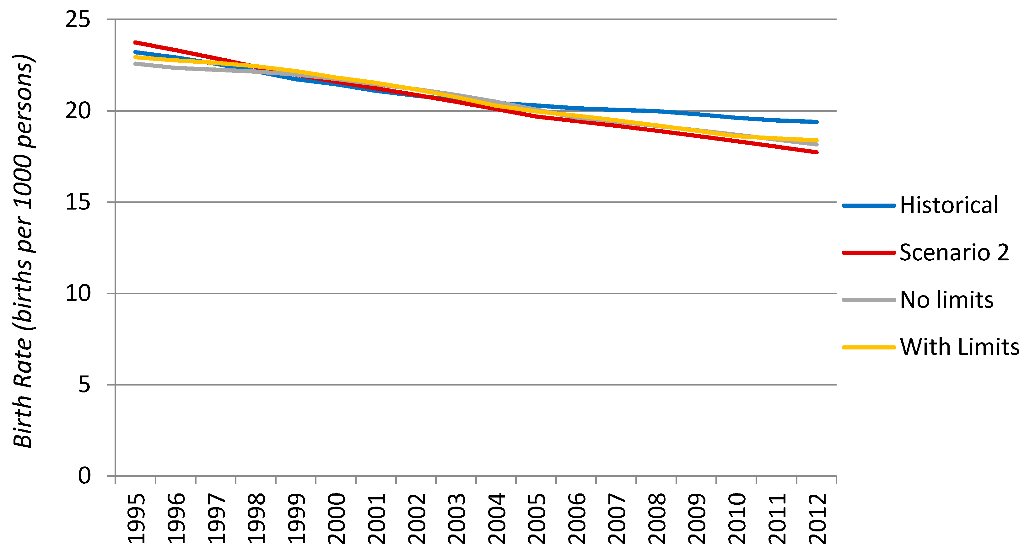
The role of this group of parameters is to link economic growth to the birth rate. The majority of newly calibrated parameters are increased slightly (Table 8) from Scenario 2. These parameters govern the response of individuals to changes in global trends and in turn influence variables such as birth rate. For example, according to the calibration of World3-03, it seems that individuals desire a slightly smaller family size but take a longer time to respond to increases in global wealth and do not perceive the benefits of improved health investment as quickly as anticipated. Given the complexity of the structure of this fraction of the model, our methodology is not able to be conclusive as to the interaction between, and absolute values of, these parameters. The interaction between these parameters within the model dynamics results in birth rates staying slightly higher for longer in the calibrated model than in the World3-03 Scenario 2.

Table 8. Result of the calibration process in relation and parameter variation in comparison with World3-03 Scenario 2.

Parameter	Value Scenario 2	Value Calibration Without Limits	Value Calibration With Limits	Variation Meaning
Desired completed family size normal	3.8	3.42	3.48	Families desire are smaller than in Scenario 2
Lifetime Multiplier from Services (*)	1 (not relevant)	0.557	0.568	The Service Output has a smaller impact on life expectancy than in Scenario 2 due to the service sector having a disproportionate output from non-health sectors (the finance sector).
Income expectation averaging time	3	3.57	3.57	Assumes that people take a longer time to adapt to changes in wealth
Health services impact delay	20	24.97	20.86	Assumes higher delays between investments and having facilities in place to provide health services
Social adjustment delay	20	26	28	Assumes that global population is a bit slower in adapting to demographic changes
Lifetime perception delay	20	23.54	28	Assumes that people perceive changes in life expectancy a bit less quickly

* parameters that have been added to World3-03 structure for the purpose of this study (see Table 4).

Table 8. Result of the calibration process in relation and parameter variation in comparison with World3-03 Scenario 2.

Parameter	Value Scenario 2	Value Calibration Without Limits	Value Calibration With Limits	Variation Meaning
Desired completed family size normal	3.8	3.42	3.48	Families desire are smaller than in Scenario 2
Lifetime Multiplier from Services (*)	1 (not relevant)	0.557	0.568	The Service Output has a smaller impact on life expectancy than in Scenario 2 due to the service sector having a disproportionate output from non-health sectors (the finance sector).
Income expectation averaging time	3	3.57	3.57	Assumes that people take a longer time to adapt to changes in wealth
Health services impact delay	20	24.97	20.86	Assumes higher delays between investments and having facilities in place to provide health services
Social adjustment delay	20	26	28	Assumes that global population is a bit slower in adapting to demographic changes
Lifetime perception delay	20	23.54	28	Assumes that people perceive changes in life expectancy a bit less quickly

* parameters that have been added to World3-03 structure for the purpose of this study (see Table 4).

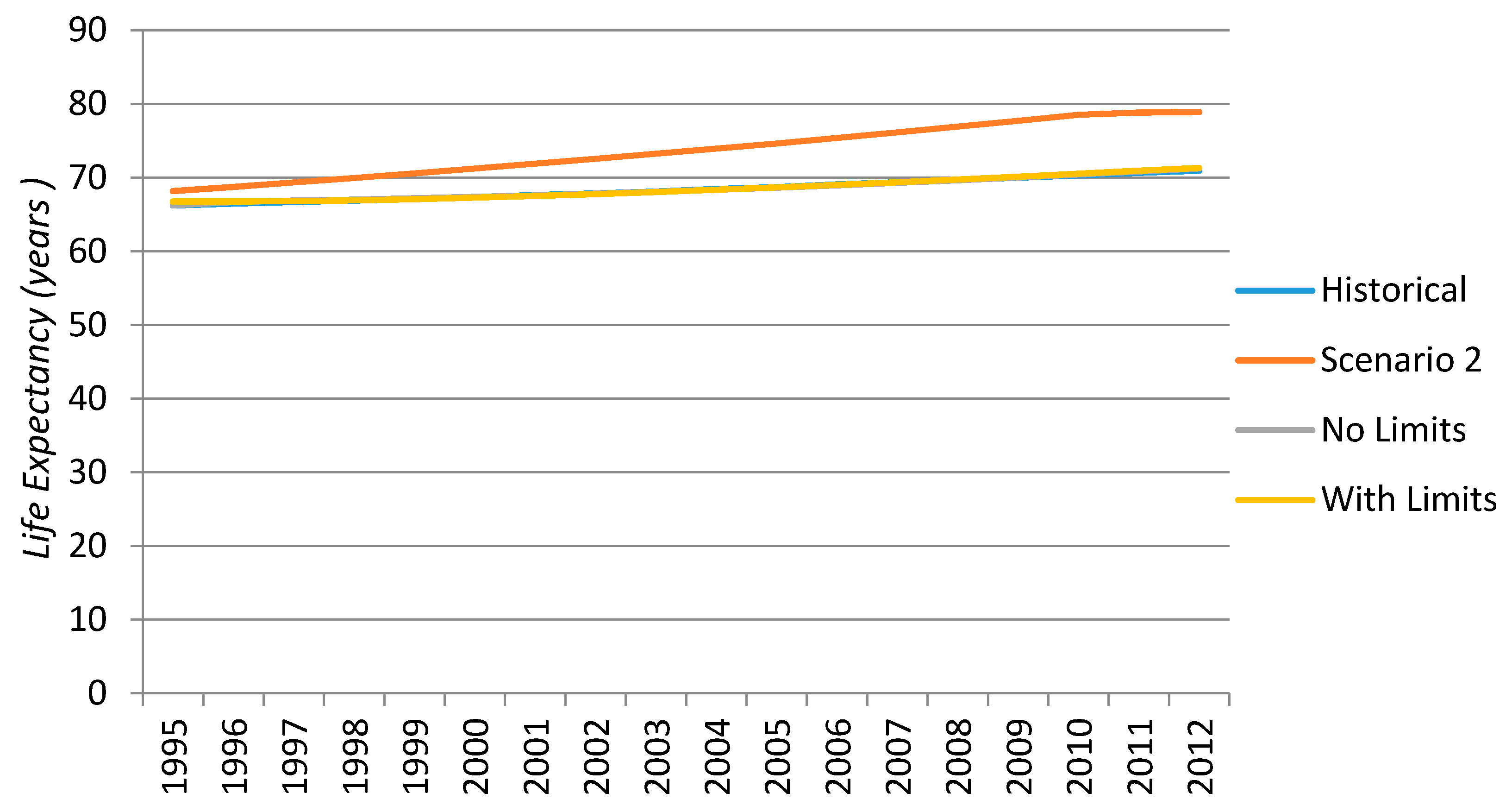
The parameter Lifetime Multiplier From Services is lower as it acts as a corrector to describe the effect of Service Output (proved to be higher than assumed in World3-03) on the health system. Its variation is meaningful only in relation to the higher level of Service Output that is seen and therefore corrects to keep the health service impact lower. World3 Scenario 2 assumes that if the world had the current level of Service Output, we would expect to have a much larger health service than we do, with a bigger impact on life expectancy. Today the much larger Service Output is dominated by the finance sector.

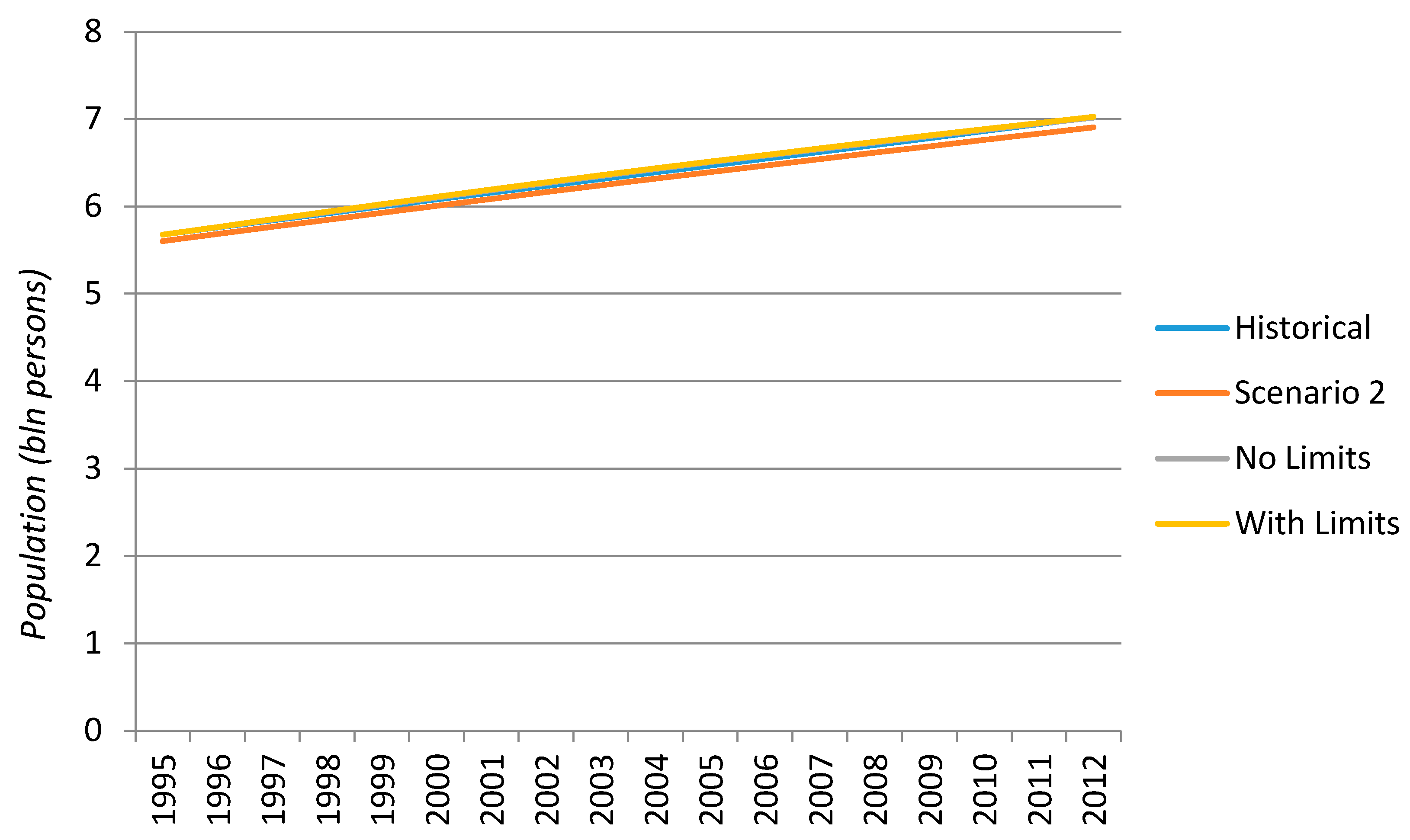
As Figure 7 shows, Population is well captured in both the calibrated model and Scenario 2. Figure 8 shows that Birth rate follows the general pathway well in both Scenario 2 and the calibrated model. However, Life Expectancy (Figure 9) in Scenario 2 was overestimated.

Figure 7. Population comparison between historic (real) data, Scenario 2 of World3 and the calibrated World3. Values in billions of people.

Figure 7. Population comparison between historic (real) data, Scenario 2 of World3 and the calibrated World3. Values in billions of people.

Figure 8. Birth rate comparison between historic (real) data, Scenario 2 of World3 and the calibrated World3.

Figure 8. Birth rate comparison between historic (real) data, Scenario 2 of World3 and the calibrated World3.

Figure 9. Life Expectancy comparison between historic (real) data, Scenario 2 of World3 and the calibrated World3.

Figure 9. Life Expectancy comparison between historic (real) data, Scenario 2 of World3 and the calibrated World3.

5. Discussion and Conclusions

The Limits to Growth (LTG) scenarios explored possible behaviour modes which highlight the nexus of economic growth and planetary boundaries. In this paper we calibrate the World3-03 model of the LTG between 1995 and 2012 to explore the differences between Scenario 2 of the LTG and the current economic system. We do not attempt to calibrate and model the overshoot and collapse scenarios presented in LTG.

Based on the World3-03 model (2004 version of the World3 model), a preliminary analysis of metadata at the global level with World3 variables was performed. In order to match data within World3 with real world data, a few scaling parameters and variables were added to the initial model structure. These additions act as conversion factors between World3 values and real world values. The resulting model was referred as World-03-Edited for the whole paper.

By calibrating World3-03 with updated time series (1995–2012), we show how the structure of the model can still provide a reliable description of some of the macro behaviours of today’s global system. However, the calibration highlighted the following differences between today’s global system when compared to the assumptions made in the LTG Scenario 2:

• Lower productivity in the industrial sector. According to World3 dynamics, human society is expected to have a lower industrial output in substitution for allocation of resources in the technological sectors to abate persistent pollution, increased resource usage efficiency and recycling, and increased food productivity of land. This is shown to be the case in the calibration and indicates that larger investments than expected have been made to mitigate some of the negative impacts of industrial output.
• Higher productivity in the service sector. The last 40 years have seen several revolutions in the growth paradigm of the global system. Telecommunications and ICT improvements determined better use of human capital, and a significant growth in the finance sector occurred.
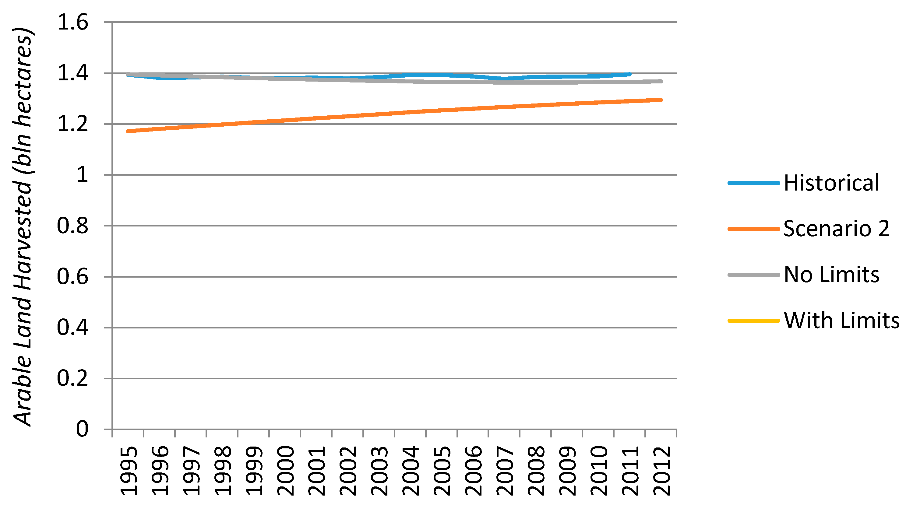
• Higher food production due to technological improvements and lower impact of food production on land erosion, even though this conclusion may be due to a different account of the processing loss within the food system in comparison to the LTG study. In addition, today the world is experiencing a steady state of arable land which is the result of a balance of two feedback loops—new land development and land erosion.

As noted, these findings are based on the underlying assumptions of the behavioural dynamics of World3 still holding true today. While a calibration of the model is shown to be able to fit current data, providing some assurance that these assumptions remain valid, further research is required to examine these in detail. In particular, we would welcome other researchers to explore this calibration method in detail and reproduce our work to ensure that the simultaneous calibration across parameters has not led to over-fitting of the data. Further research is also required to calibrate parameters that are associated with the overshoot scenarios presented in LTG not explored in this paper. In particular, to explore these future scenarios, further research is required to quantify limits on resource availability and the impacts of pollution on agricultural productivity.

As shown in this paper, future models based on World3 would benefit from building in additional behaviours that are under-represented in the current model. In particular, the service sector is under-represented in World3-03. Given the dominance in today’s global economy of the finance sector, a more detailed analysis of the behaviour modes of finance, and in particular banks, is required to be able to more accurately build further scenarios. This is the subject of our ongoing research.

This paper aims to be a reference point to highlight the difference between the assumptions made about the world in 1972 and today’s world. In particular, the service sector is much larger than anticipated and we have invested to alleviate some of the impacts of pollution. While World3 can be calibrated to fit today’s global trends, it was not designed to model the behaviour of the service sector as it currently is. Therefore, new models able to capture the dynamics of the knowledge economy and finance sector, which are now the driving forces of the economy, can help better model current dynamics and, importantly, shed light on future pathways.

While society has invested in mitigation of some of the impacts of our industrial output, we still live on a finite planet. Based on this paper, we cannot be sure how and when the limits will be reached, but the growth paradigm is still based on material consumption, and the planet is still limited in terms of land availability and material resources and cannot be polluted forever.