
Spatial Modeling of Urban Vegetation and Land Surface Temperature: A Case Study of Beijing


Abstract
:1. Introduction
2. Data, Study Site and Methods
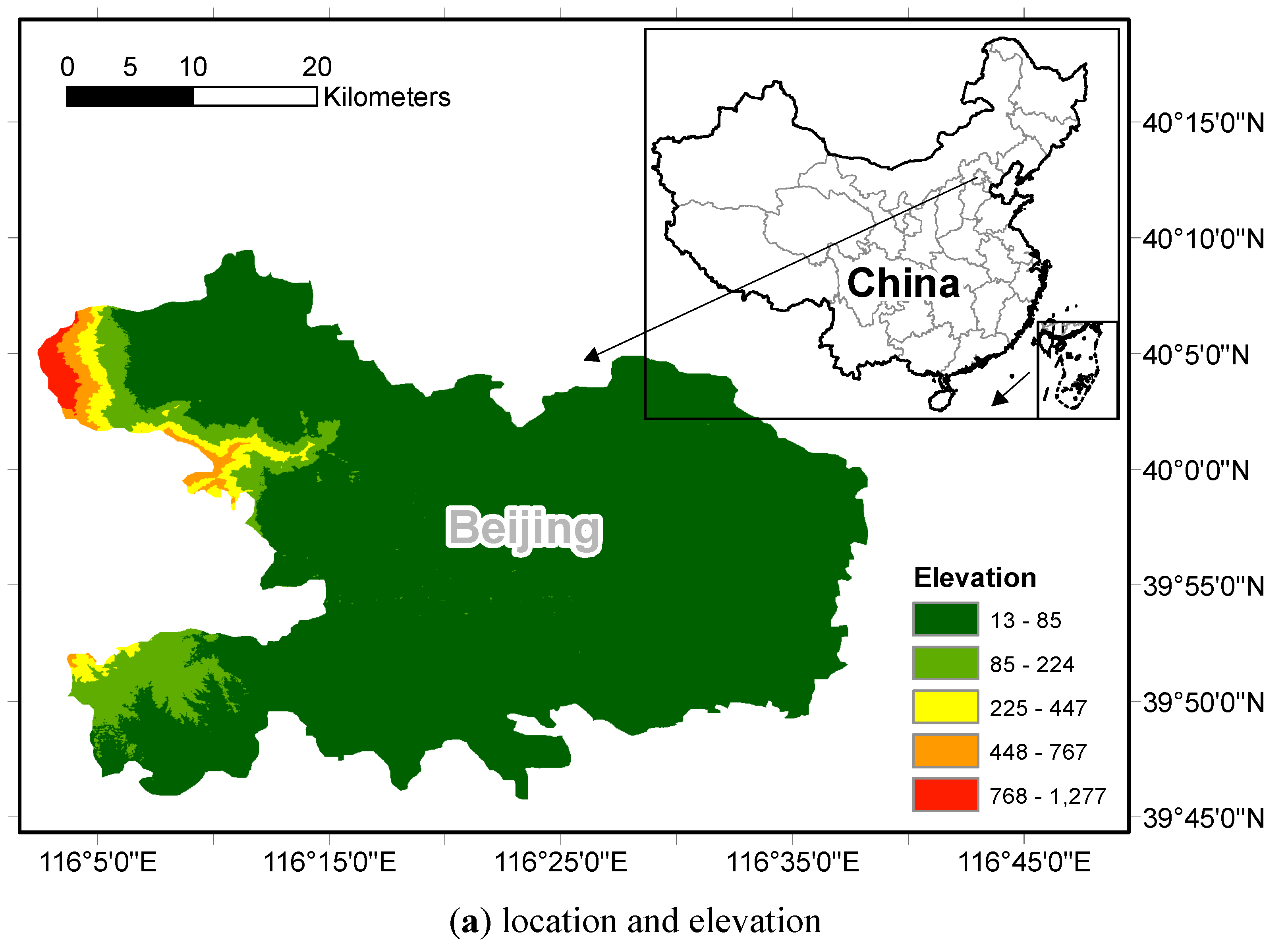
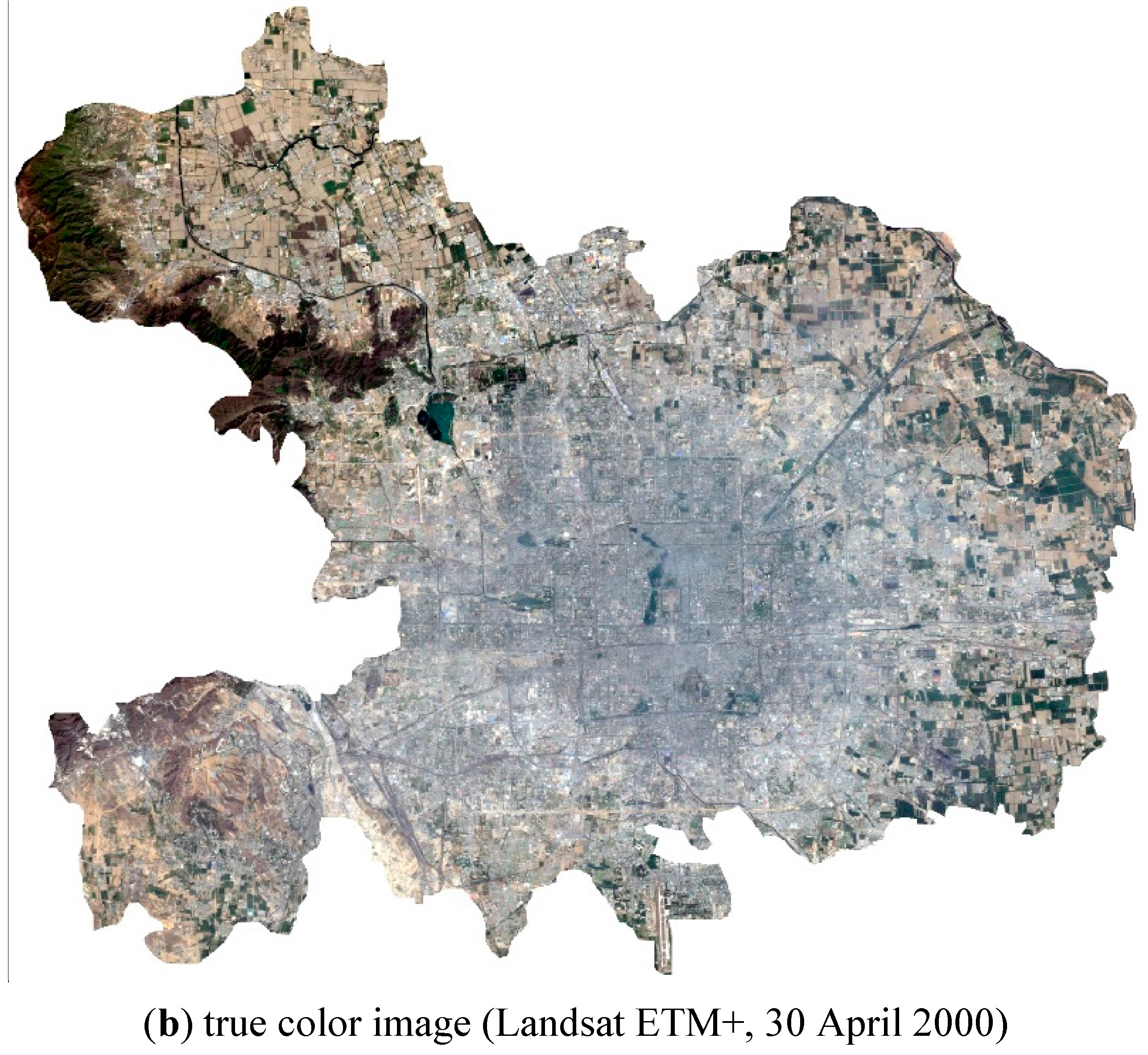
2.1. Data and Study Site

| Data Type | Acquisition date | Precipitation before acquisition date (mm) * | |
|---|---|---|---|
| 1 | Landsat TM | 13 May 1990 | 1 |
| 2 | Landsat TM | 7 September 1992 | 0 (159 the day before) |
| 3 | Landsat TM | 8 May 1994 | 0 |
| 4 | Landsat TM | 21 September 1997 | 0 |
| 5 | Landsat TM | 6 May 1999 | 0 |
| 6 | Landsat ETM+ | 1 July 1999 | 0 |
| 7 | Landsat ETM+ | 30 April 2000 | 13 |
| 8 | Landsat ETM+ | 19 May 2001 | 0 |
| 9 | Terra ASTER | 4 June 2001 | 0 |
| 10 | Terra ASTER | 12 June 2004 | 0 |
| 11 | Terra ASTER | 22 April 2006 | 0 |
| 12 | Terra ASTER | 8 August 2007 | 68 |
2.2. Estimation of Vegetation Cover
2.2.1. NDVI
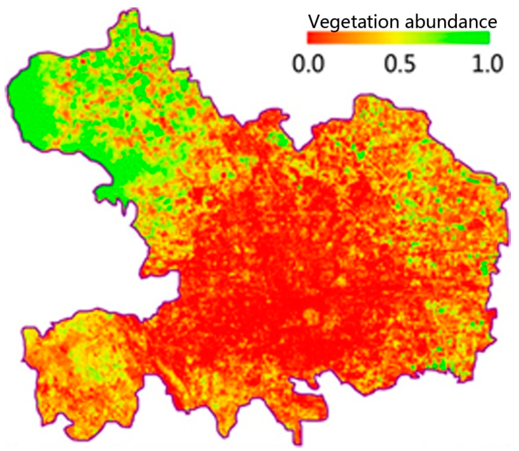
2.2.2. Vegetation Abundance

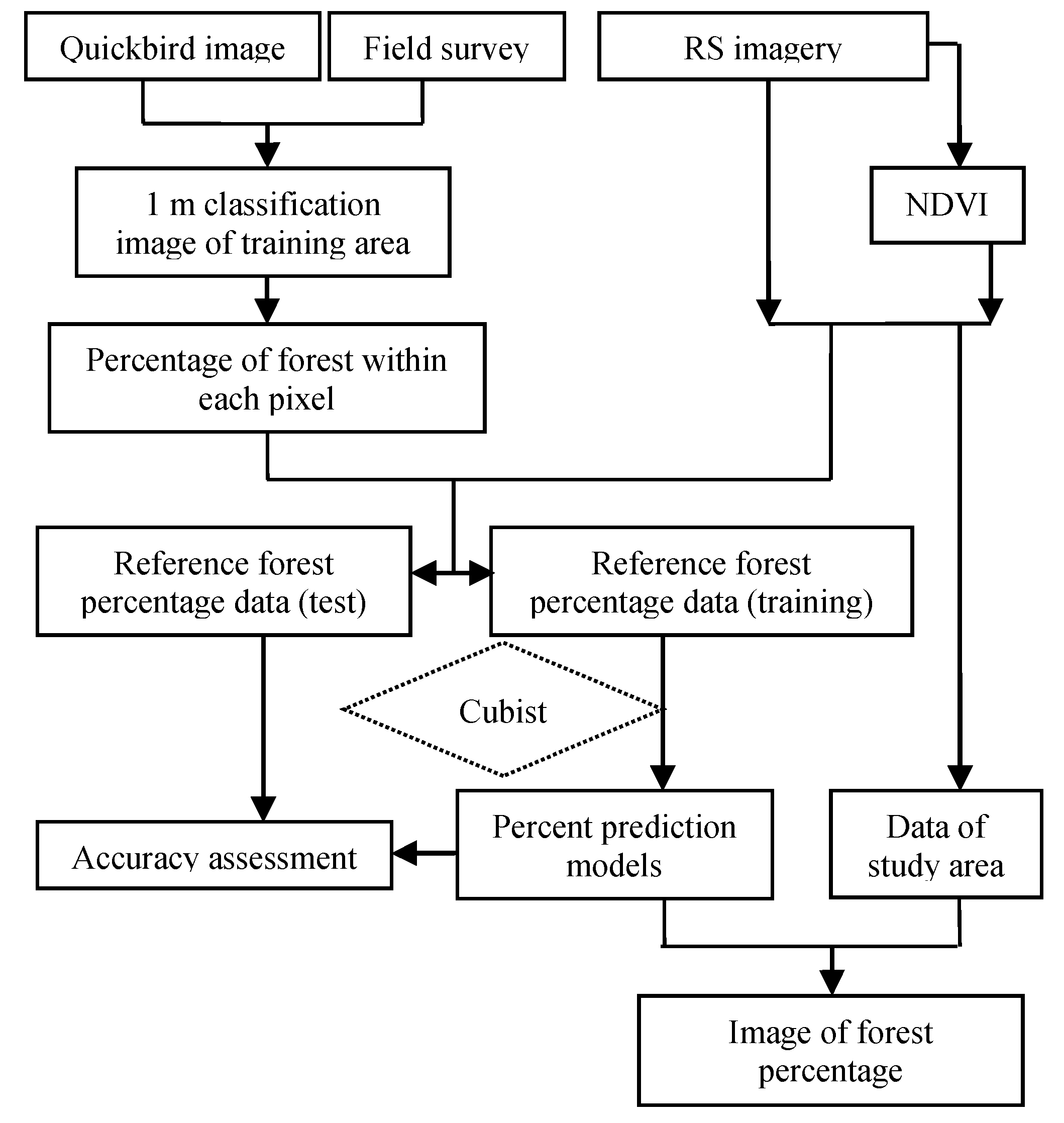
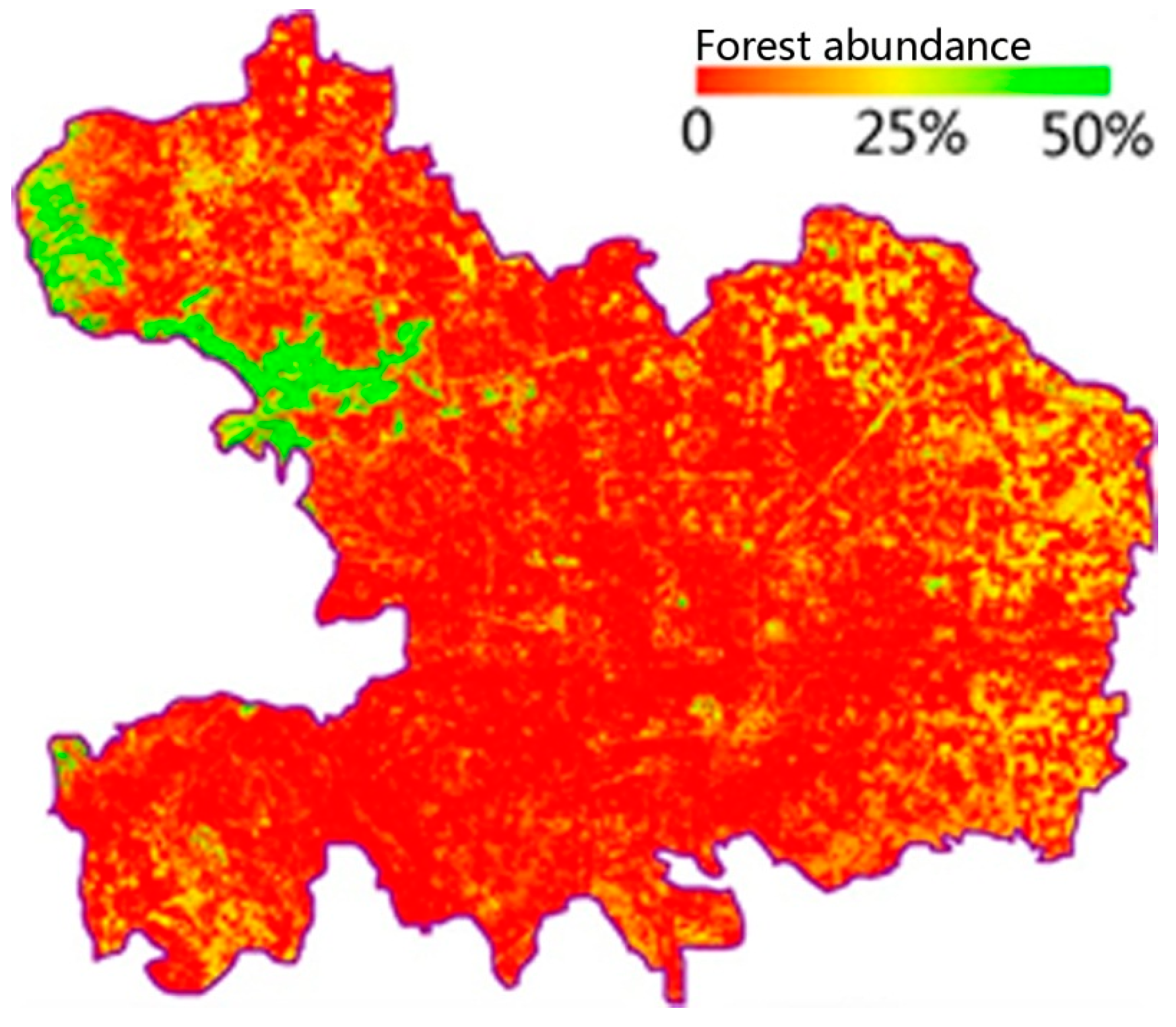
2.2.3. Forest Abundance


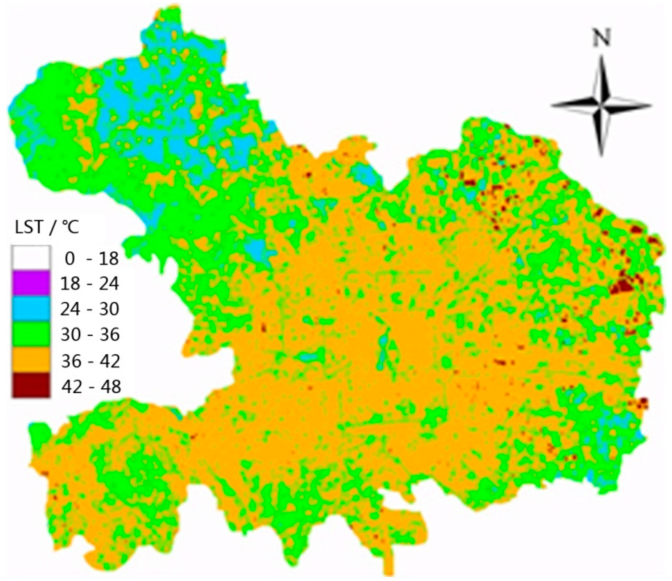
2.3. LST Retrieval
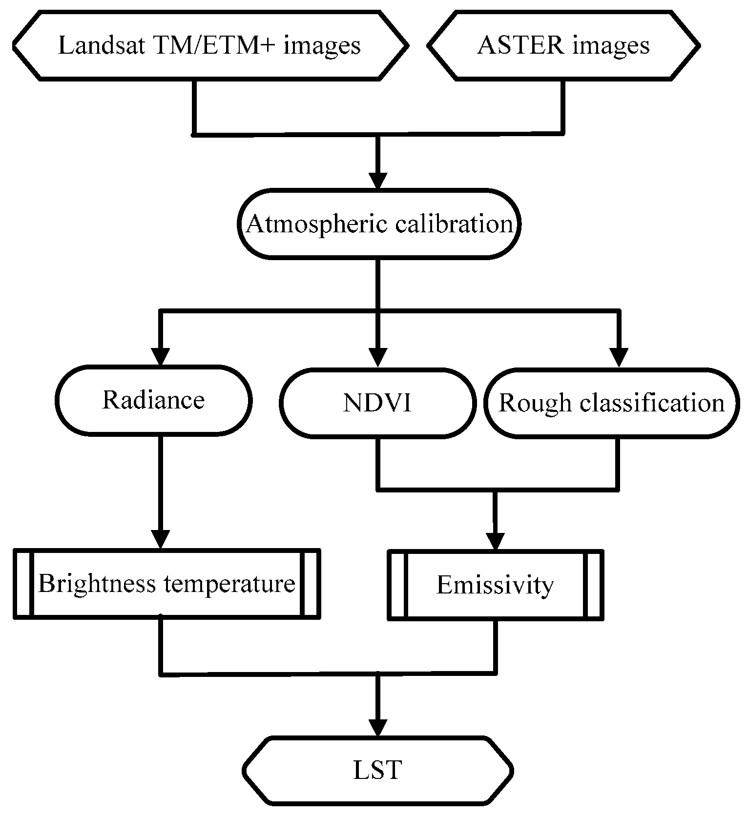
2.3.1. Land Surface Emissivity Estimation
2.3.2. LST Calculation from Landsat TM/ETM+ Imagery

2.3.3. LST Calculation from Terra ASTER Images
2.4. Coupling Relationship Analysis
- –
- : , are negative correlations, absolutely negative correlations if ;
- –
- : , are absolutely not correlated;
- –
- : , are in positively correlated, and absolutely positively correlated if ;
3. Results and Discussion
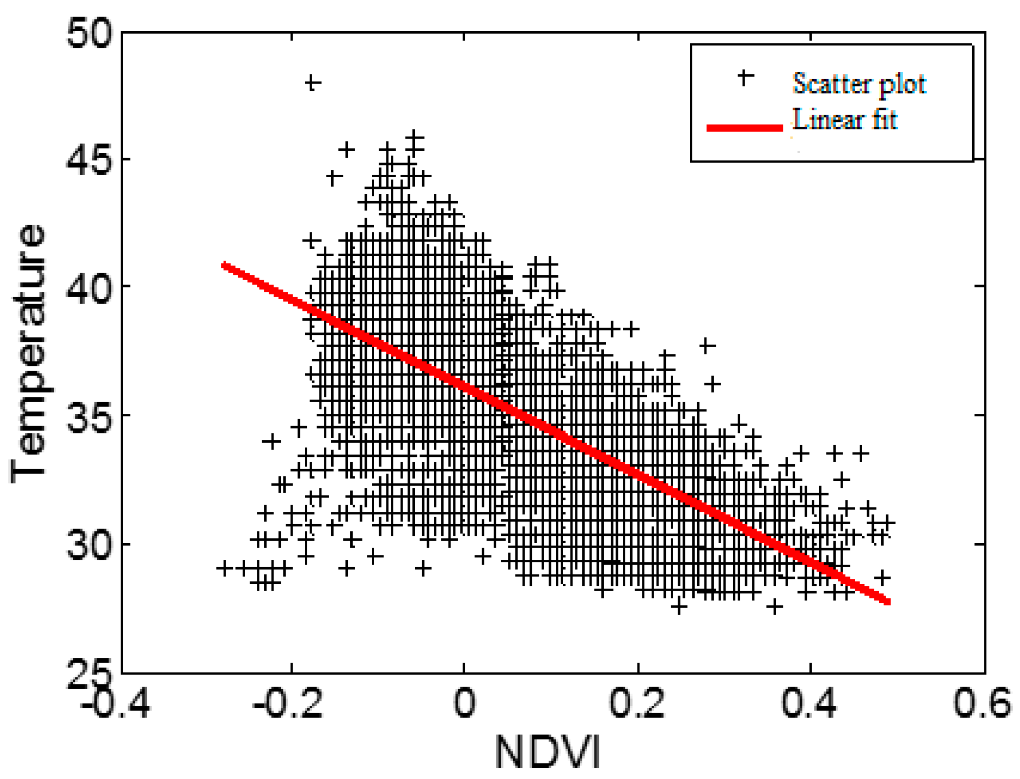
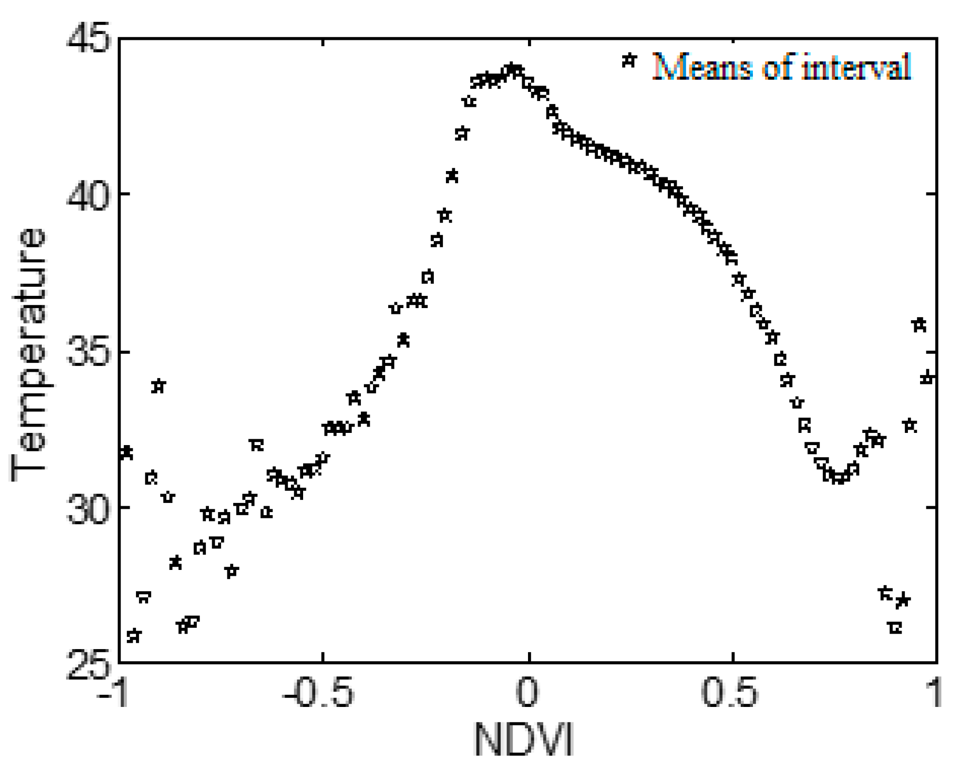
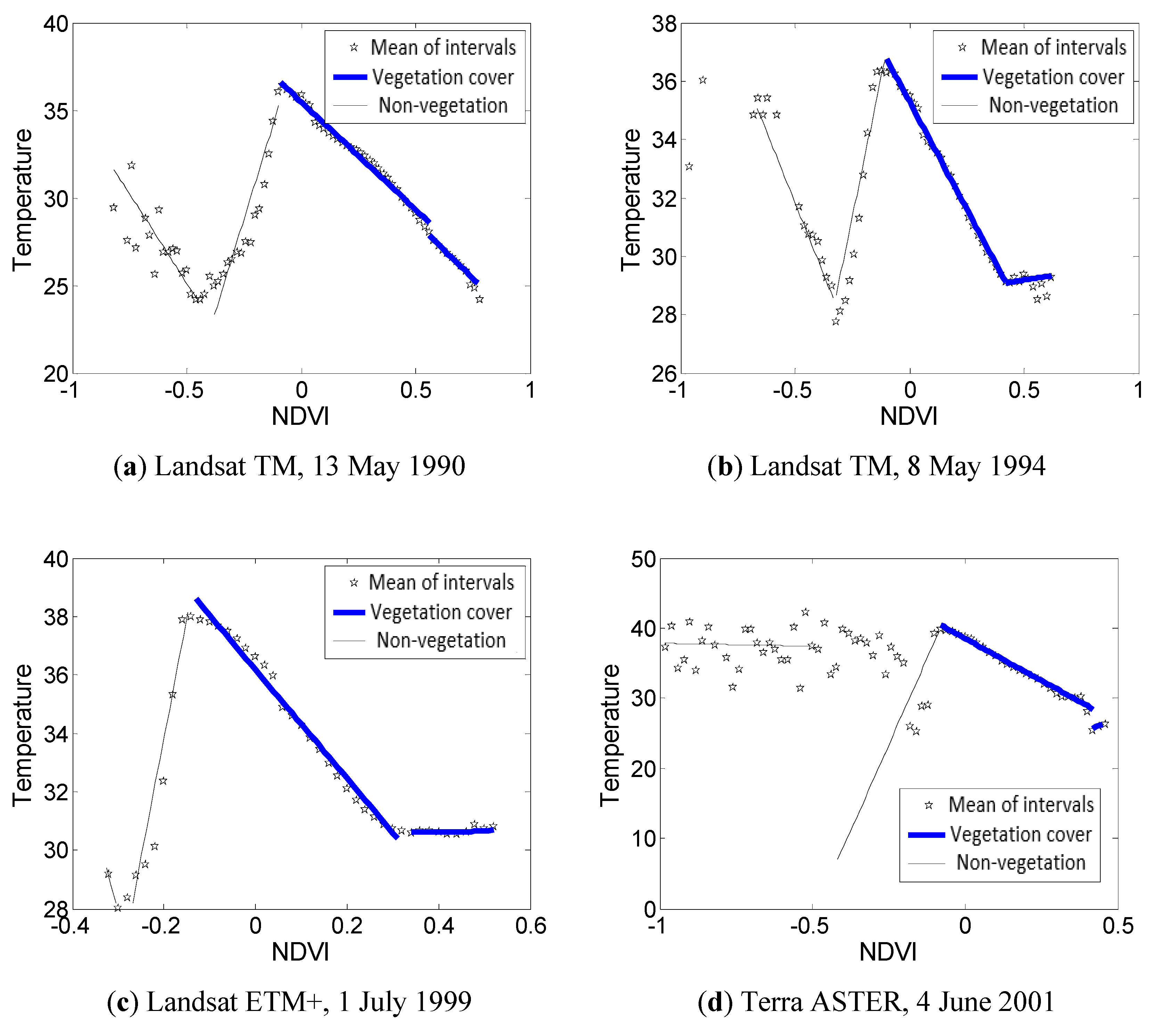
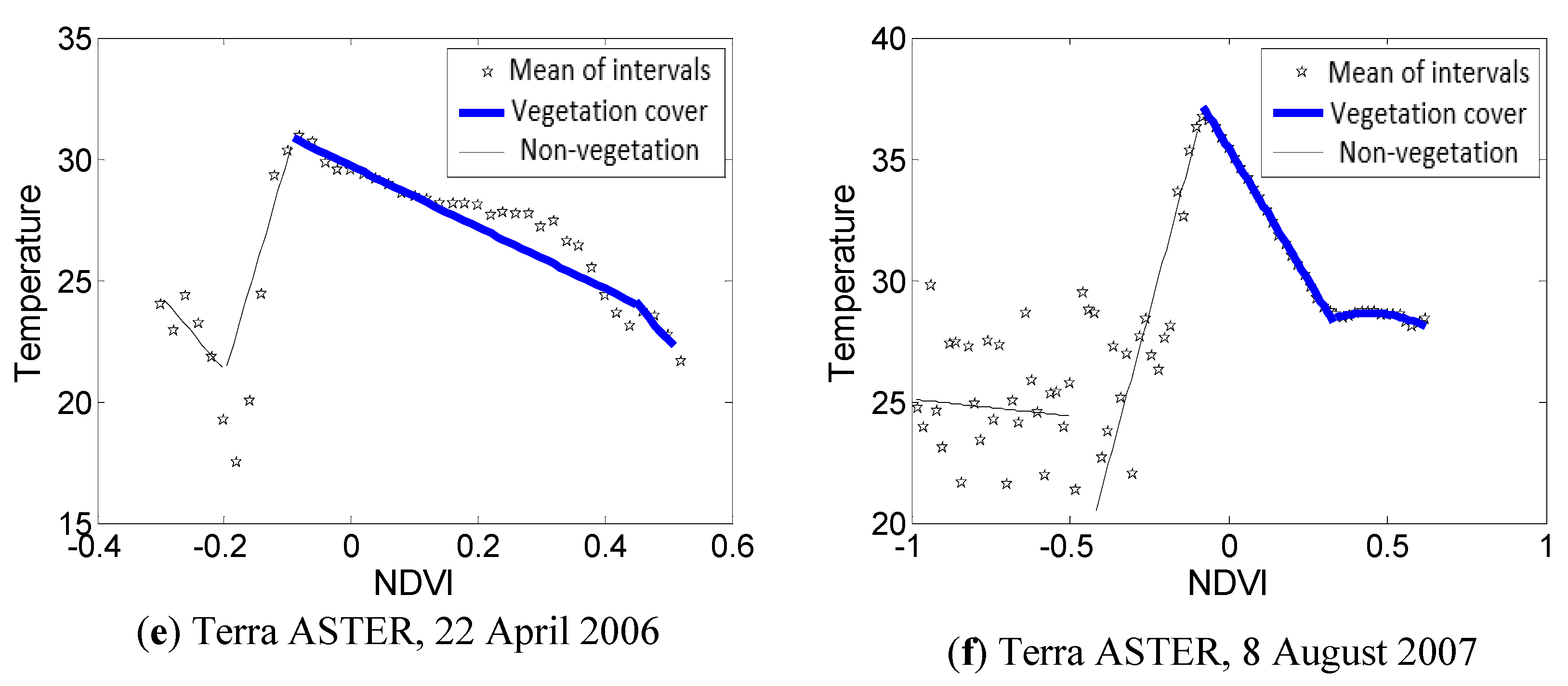
3.1. NDVI and LST


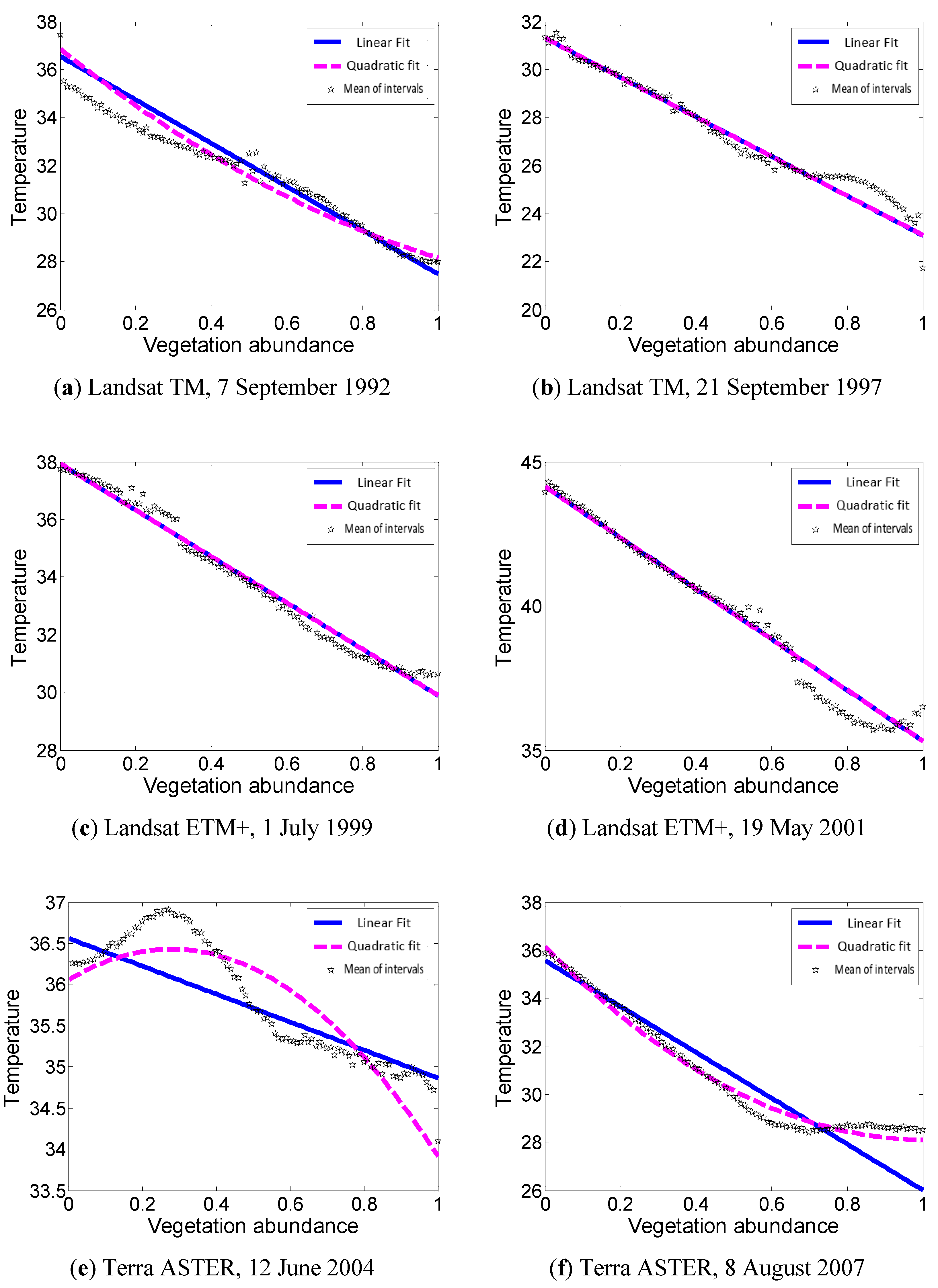
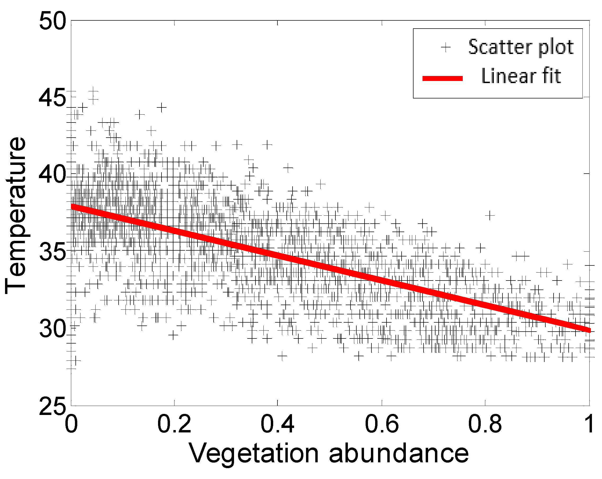
3.2. Urban Vegetation Abundance and LST

- (1).
- Directly based on analysis of all pixels, the value of UVA and LST are linearly fitted and quadratically fitted; Pearson’s correlation coefficients are calculated for all pixel values (and presented in Table 3);
- (2).
- The range of UVA, [0, 100%], is divided into 100 intervals. The mean values of the 100 intervals and the corresponding mean values of LST are also linearly fitted; Pearson’s correlation coefficients are calculated for the mean values (and presented in Table 3).
- (1).
- The monomial coefficients are approximate, with the mean values from 12 images being between −7.1116 and −7.3429, which also show the numeric effect of vegetation in decreasing LST.
- (2).
- The values of differ greatly. For the polynomial fitting for all 12 images, the mean values of are 0.2982 and 0.3055. For the linear fitting and quadratic fitting, the values are much smaller than 0.9448. This also demonstrates that LST is influenced by vegetation, whereas it is also influenced by other factors, including elevation mentioned above.
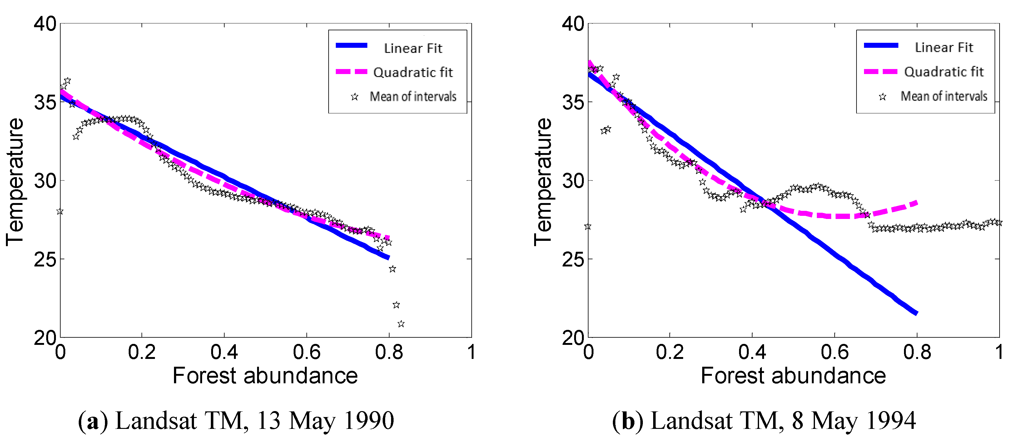
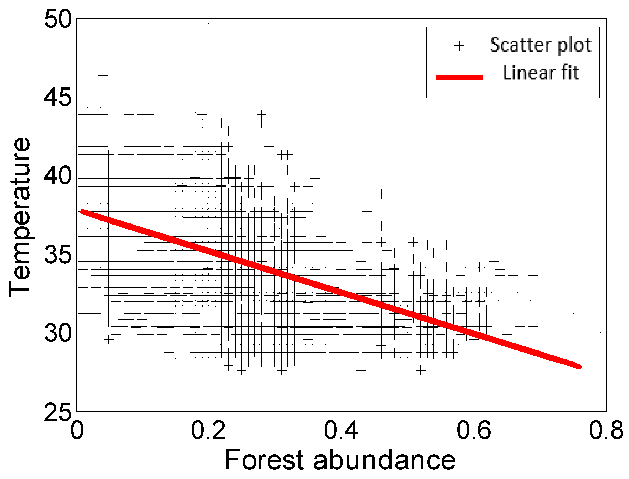
3.3. Urban Forest Abundance and LST

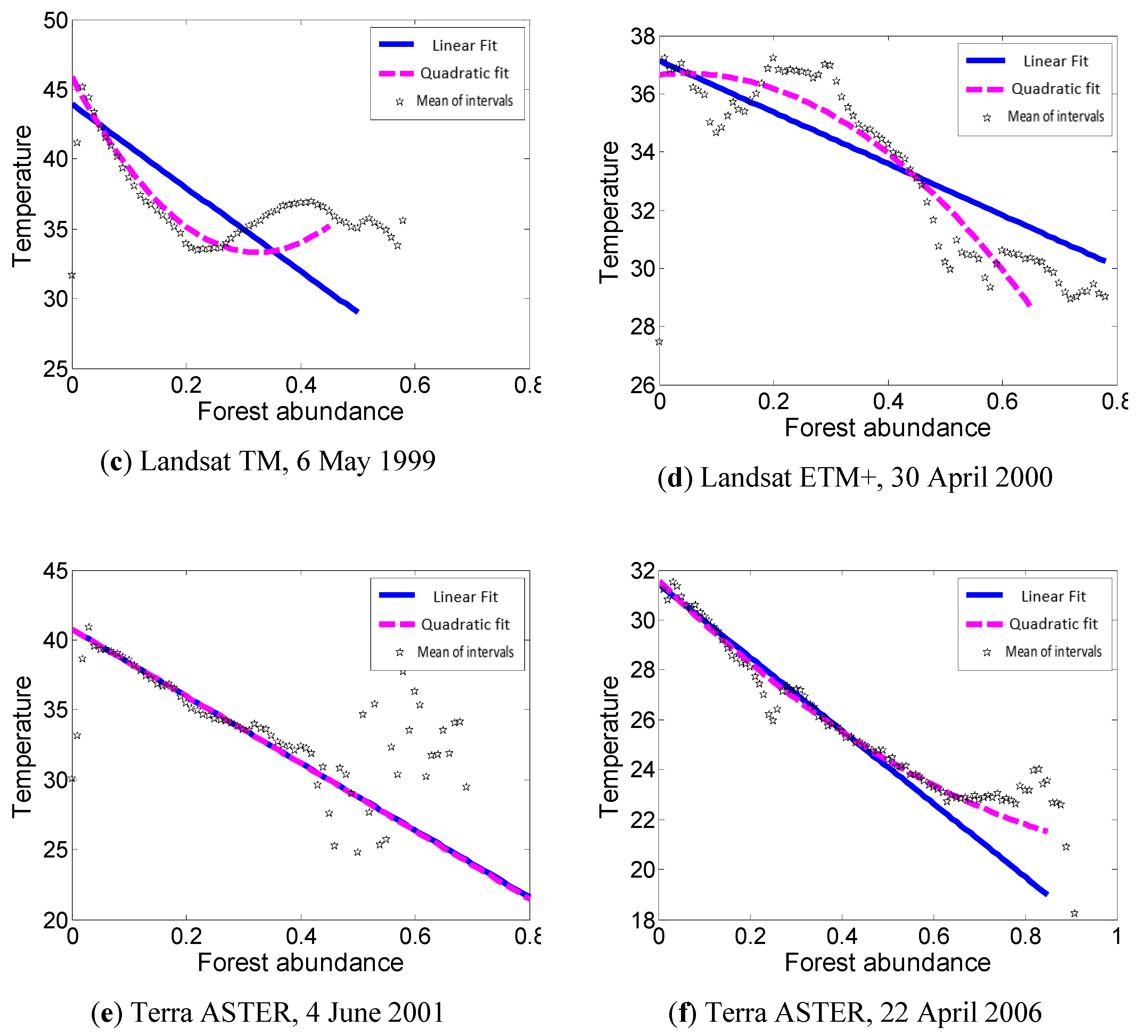
- (1).
- Based on analysis of all pixels, the values of UFA and LST are linearly fitted and quadratically fitted. Pearson's correlation coefficients are calculated for all pixel values (Table 4);
- (2).
- The range of UFA, [0, 100%], is divided into 100 intervals. The mean values of the 100 intervals and the corresponding mean values of LST are also linearly fitted. Pearson's correlation coefficients are calculated for the mean values (Table 4).
- –
- There is not very much urban forest in the study area;
- –
- Some western areas are mountainous areas covered with forest. So elements other that the UFA, e.g., elevation, soil moisture, also influence LST.
- –
- In the study area, there are various types of trees, which play different roles in decreasing LST;
- –
- There exist some errors in the calculation of UFA;
3.4. Scale Effects
3.4.1. NDVI–LST
3.4.2. UVA–LST
3.4.3. UFA–LST
3.4.4. Summary
| Thresholds of NDVI | Fit of LST and NDVI NDVI ∈ (Bare soil, Vegetation cover) | Fit of LST and mean NDVI of each interval NDVI ∈ (Bare soil, Vegetation cover) | Pearson’s correlation coefficients | ||||||||
|---|---|---|---|---|---|---|---|---|---|---|---|
| Water | Bare Soil | Vegetation Cover | Monomial coefficient | Constant | Monomial coefficient | Constant | All Pixels | NDVI ∈ (Bare soil, Vegetation cover) | |||
| 1990 TM | −0.45 | −0.09 | 0.56 | –12.2928 | 35.4764 | 0.3408 | –12.4806 | 35.5156 | 0.9867 | –0.6158 | –0.9934 |
| 1992 TM | −0.2 | –0.05 | 0.58 | –17.9615 | 37.7120 | 0.6989 | –17.9276 | 37.7203 | 0.9790 | –0.8264 | –0.9894 |
| 1994 TM | −0.32 | –0.1 | 0.42 | –14.7138 | 35.2906 | 0.2798 | –14.8015 | 35.2758 | 0.9951 | –0.4987 | –0.9976 |
| 1997 TM | –0.8 | –0.15 | 0.74 | –7.9520 | 30.9888 | 0.3002 | –8.0716 | 31.0836 | 0.9491 | –0.5943 | –0.9742 |
| 1999 TM | –0.7 | –0.05 | 0.78 | –13.7330 | 43.7044 | 0.3765 | –15.5863 | 44.3581 | 0.9313 | –0.5070 | –0.9650 |
| 1999 ETM+ | –0.3 | –0.14 | 0.34 | –18.6408 | 36.1800 | 0.5177 | –18.2092 | 36.1230 | 0.9812 | –0.7058 | –0.9906 |
| 2000 ETM+ | –0.8 | –0.33 | 0.32 | –12.2349 | 33.5019 | 0.2319 | –14.3637 | 33.3297 | 0.9702 | –0.3212 | –0.9850 |
| 2001 ETM+ | –0.58 | –0.32 | 0.2 | –17.1152 | 38.9377 | 0.3141 | –17.2958 | 38.9225 | 0.9902 | –0.4912 | –0.9951 |
| 2001 ASTER | –0.5 | –0.08 | 0.42 | –24.0389 | 38.5407 | 0.1771 | –25.6857 | 38.5730 | 0.9748 | –0.3923 | –0.9873 |
| 2004 ASTER | –0.23 | –0.09 | 0.5 | –18.0121 | 35.2307 | 0.0566 | –11.8544 | 35.2114 | 0.4391 | –0.1333 | –0.6626 |
| 2006 ASTER | –0.2 | –0.09 | 0.45 | –12.6498 | 29.7159 | 0.0347 | –11.3023 | 29.8595 | 0.8687 | –0.1394 | –0.9320 |
| 2007 ASTER | –0.5 | –0.09 | 0.34 | –21.6386 | 35.4286 | 0.3402 | –21.1473 | 35.3610 | 0.9966 | –0.6307 | –0.9983 |
| Mean | −0.47 | −0.13 | 0.47 | −15.9153 | 35.8923 | 0.3057 | −15.7272 | 35.9445 | 0.9218 | −0.4880 | −0.9559 |
| Fit of mean of intervals | Linear fit | Quadratic fit | Pearson’s correlation coefficients | |||||||||||
|---|---|---|---|---|---|---|---|---|---|---|---|---|---|---|
| Monomial coefficient | Constant | Monomial coefficient | Constant | Quadratic coefficient | Monomial coefficient | Constant | Pixel value | Mean of intervals | ||||||
| 1990 TM | −8.0942 | 35.6088 | 0.9781 | −8.1612 | 35.5866 | 0.4100 | −1.3365 | −7.0286 | 35.4868 | 0.4109 | −0.6403 | −0.9890 | ||
| 1992 TM | −7.4503 | 35.4107 | 0.9744 | −9.0569 | 36.5539 | 0.6626 | 3.8315 | −12.5202 | 36.8455 | 0.6698 | −0.8140 | −0.9871 | ||
| 1994 TM | −6.7556 | 36.4812 | 0.9936 | −6.5170 | 36.3318 | 0.2760 | −1.5332 | −5.2720 | 36.2340 | 0.2772 | −0.5253 | −0.9968 | ||
| 1997 TM | −7.5678 | 31.1136 | 0.9717 | −8.2169 | 31.3132 | 0.4133 | 0.0570 | −8.2664 | 31.3178 | 0.4133 | −0.6429 | −0.9858 | ||
| 1999 TM | −12.2816 | 44.9093 | 0.9340 | −10.2816 | 43.8315 | 0.3177 | −9.4809 | −2.6838 | 43.2458 | 0.3382 | −0.5637 | −0.9665 | ||
| 1999 ETM+ | −8.2592 | 38.0257 | 0.9845 | −8.0378 | 37.9278 | 0.5256 | 0.0362 | −8.0676 | 37.9303 | 0.5256 | −0.7250 | −0.9922 | ||
| 2000 ETM+ | −8.4197 | 38.0622 | 0.9466 | −6.0629 | 37.0959 | 0.1504 | −7.5576 | −0.6721 | 36.7461 | 0.1701 | −0.3878 | −0.9730 | ||
| 2001 ETM+ | −9.3462 | 44.2796 | 0.9772 | −8.8133 | 44.1252 | 0.2892 | 0.0476 | −8.8476 | 44.1275 | 0.2892 | −0.5378 | −0.9885 | ||
| 2001 ASTER | −6.7738 | 40.2789 | 0.9854 | −6.0567 | 39.8884 | 0.1332 | −4.9580 | −1.9717 | 39.4737 | 0.1409 | −0.3650 | −0.9927 | ||
| 2004 ASTER | −2.2155 | 36.9150 | 0.7868 | −1.6963 | 36.5617 | 0.0199 | −4.8204 | 2.6790 | 36.0580 | 0.0339 | −0.1409 | −0.8870 | ||
| 2006 ASTER | −2.9451 | 30.6702 | 0.9169 | −2.8875 | 30.6096 | 0.0236 | −0.8655 | −2.2508 | 30.5558 | 0.0238 | −0.1536 | −0.9576 | ||
| 2007 ASTER | −8.0054 | 34.8716 | 0.8888 | −9.5506 | 35.5724 | 0.3568 | 7.8842 | −15.9222 | 36.1484 | 0.3725 | −0.5973 | −0.9427 | ||
| Mean | −7.3429 | 37.2189 | 0.9448 | −7.1116 | 37.1165 | 0.2982 | −1.5580 | −5.9020 | 37.0141 | 0.3055 | −0.5078 | −0.9716 | ||
| Fit of mean of intervals | Linear fit | Quadratic fit | Pearson’s correlation coefficients | ||||||||||||
|---|---|---|---|---|---|---|---|---|---|---|---|---|---|---|---|
| Monomial coefficient | Constant | Monomial coefficient | Constant | Quadratic coefficient | Monomial coefficient | Constant | Pixel value | Mean of intervals | |||||||
| 1990 TM | −11.6010 | 34.5226 | 0.8539 | −12.9336 | 35.3560 | 0.4494 | 8.0636 | −18.1931 | 35.6938 | 0.4563 | −0.6704 | −0.9241 | |||
| 1992 TM | −11.1884 | 36.4250 | 0.9112 | −11.5014 | 36.5410 | 0.6489 | 9.1876 | −18.6565 | 37.1977 | 0.6595 | −0.8055 | −0.9546 | |||
| 1994 TM | −7.7636 | 33.3574 | 0.7008 | −19.1950 | 36.8026 | 0.4248 | 26.3016 | −32.2491 | 37.5484 | 0.4611 | −0.6517 | −0.8372 | |||
| 1997 TM | −7.4677 | 27.6790 | 0.7026 | −13.8285 | 30.1439 | 0.3583 | 21.9188 | −29.4157 | 31.1497 | 0.4271 | −0.5986 | −0.8382 | |||
| 1999 TM | −8.1828 | 38.8291 | 0.2550 | −29.8147 | 43.9045 | 0.3698 | 119.6103 | −77.4715 | 45.8674 | 0.4924 | −0.6081 | −0.5049 | |||
| 1999 ETM+ | −7.6300 | 36.2626 | 0.7260 | −12.8932 | 37.7325 | 0.3424 | 8.6190 | −17.2400 | 38.0232 | 0.3475 | −0.5851 | −0.8520 | |||
| 2000 ETM+ | −11.0101 | 37.5955 | 0.7022 | −8.8423 | 37.1371 | 0.1636 | −22.1424 | 2.1104 | 36.6507 | 0.1895 | −0.4044 | −0.8379 | |||
| 2001 ETM+ | −5.4096 | 41.3349 | 0.6384 | −9.9076 | 43.6218 | 0.2384 | 15.5237 | −21.7775 | 44.2037 | 0.2963 | −0.4882 | −0.7990 | |||
| 2001 ASTER | −11.3096 | 37.6455 | 0.3905 | −23.9683 | 40.7667 | 0.1445 | −0.3147 | −23.8586 | 40.7600 | 0.1445 | −0.3801 | −0.6249 | |||
| 2004 ASTER | −10.1165 | 36.0246 | 0.3953 | −12.9336 | 37.4387 | 0.0859 | −18.5385 | −5.1195 | 36.9165 | 0.0901 | −0.2931 | −0.6287 | |||
| 2006 ASTER | −10.3612 | 30.2757 | 0.9011 | −14.6337 | 31.4104 | 0.1888 | 7.2639 | −18.0127 | 31.5644 | 0.1908 | −0.4345 | −0.9493 | |||
| 2007 ASTER | −23.4166 | 38.5703 | 0.7096 | −13.6613 | 36.4287 | 0.3683 | 18.8188 | −25.2949 | 37.4774 | 0.3874 | −0.6069 | −0.8424 | |||
| Mean | −10.4548 | 35.7102 | 0.6572 | −15.3428 | 37.2737 | 0.3152 | 16.1926 | −23.7649 | 37.7544 | 0.3452 | −0.5439 | −0.7994 | |||
| Resolution | 13 May 1990, Landsat TM | 19 May 2001, Landsat ETM+ | 8 August 2007, ASTER | |||||||
|---|---|---|---|---|---|---|---|---|---|---|
| Linear Fit, Monomial coefficient | Linear Fit, | Pearson’s correlation coefficients | Linear Fit, Monomial coefficient | Linear Fit, | Pearson’s correlation coefficients | Linear Fit, Monomial coefficient | Linear Fit, | Pearson’s correlation coefficients | ||
| NDVI and LST | 30 M | −12.29 | 0.34 | –0.62 | –17.12 | 0.31 | –0.49 | –21.64 | 0.34 | –0.63 |
| 60 M | −12.92 | 0.30 | –0.58 | –17.37 | 0.30 | –0.36 | –23.06 | 0.36 | –0.55 | |
| 90 M | –13.25 | 0.25 | –0.54 | –17.55 | 0.31 | –0.18 | –23.65 | 0.38 | –0.39 | |
| 120 M | –13.16 | 0.20 | –0.49 | –17.63 | 0.31 | –0.02 | –24.15 | 0.39 | –0.26 | |
| 240 M | –11.57 | 0.09 | –0.32 | –16.96 | 0.28 | 0.37 | –24.11 | 0.39 | 0.16 | |
| 480 M | –5.95 | 0.01 | –0.12 | –15.92 | 0.24 | 0.66 | –22.74 | 0.38 | 0.55 | |
| 960 M | 6.89 | 0.01 | 0.09 | –14.87 | 0.23 | 0.83 | –20.38 | 0.33 | 0.77 | |
| Vegetation and LST | 30 M | –8.16 | 0.41 | –0.64 | –8.81 | 0.29 | –0.54 | –9.55 | 0.36 | –0.60 |
| 60 M | –8.35 | 0.35 | –0.59 | –8.99 | 0.23 | –0.48 | –10.14 | 0.37 | –0.61 | |
| 90 M | –8.62 | 0.29 | –0.54 | –8.84 | 0.17 | –0.41 | –10.40 | 0.33 | –0.57 | |
| 120 M | –8.64 | 0.24 | –0.49 | –8.56 | 0.12 | –0.35 | –10.50 | 0.29 | –0.54 | |
| 240 M | –7.53 | 0.10 | –0.32 | –6.79 | 0.04 | –0.20 | –9.57 | 0.16 | –0.40 | |
| 480 M | –3.35 | 0.01 | –0.10 | –2.12 | 0.00 | –0.04 | –6.19 | 0.04 | –0.19 | |
| 960 M | 6.53 | 0.02 | 0.13 | –6.36 | 0.04 | –0.19 | 1.11 | 0.00 | 0.02 | |
| Forest and LST | 30 M | –12.93 | 0.45 | –0.67 | –9.91 | 0.24 | –0.49 | –13.66 | 0.37 | –0.61 |
| 60 M | –14.01 | 0.42 | –0.65 | –10.86 | 0.22 | –0.47 | –14.58 | 0.33 | –0.58 | |
| 90 M | –14.52 | 0.37 | –0.61 | –11.08 | 0.18 | –0.43 | –14.73 | 0.29 | –0.53 | |
| 120 M | –14.64 | 0.31 | –0.56 | –10.99 | 0.15 | –0.38 | –14.65 | 0.25 | –0.50 | |
| 240 M | –14.06 | 0.17 | –0.41 | –10.17 | 0.07 | –0.27 | –12.85 | 0.13 | –0.35 | |
| 480 M | –10.50 | 0.05 | –0.21 | –7.37 | 0.02 | –0.14 | –7.42 | 0.02 | –0.15 | |
| 960 M | 0.14 | 0.00 | 0.00 | –2.25 | 0.00 | –0.03 | 1.93 | 0.00 | 0.03 | |
4. Conclusions
Acknowledgments
Author Contributions
Conflicts of Interest
References
- Dai, X.; Guo, Z.; Zhang, L.; Li, D. Spatiotemporal Exploratory Analysis of Urban Surface Temperature Field in Shanghai, China. Stoch. Environ. Res. Risk. Assess. 2010, 24, 247–257. [Google Scholar] [CrossRef]
- Wei, Y.; Ye, X. Beyond Convergence: Space, Scale, and Regional Inequality in China. J. Econ. Soc. Geogr. 2009, 100, 59–80. [Google Scholar] [CrossRef]
- Yue, W.; Liu, Y.; Fan, X.; Ye, P.; Wu, C. Assessing Spatial Pattern of Urban Thermal Environment in Shanghai, China. Stoch. Environ. Res. Risk. Assess. 2012, 26, 899–911. [Google Scholar] [CrossRef]
- Weng, Q. Thermal infrared remote sensing for urban climate and environmental studies: Methods, applications, and trends. ISPRS J. Photogramm 2009, 64, 335–344. [Google Scholar] [CrossRef]
- Yang, W.; Li, F.; Wang, R.; Hu, D. Ecological benefits assessment and spatial modeling of urban ecosystem for controlling urban sprawl in Eastern Beijing, China. Ecol. Complex. 2011, 81, 153–160. [Google Scholar] [CrossRef]
- Weng, Q.; Rajasekar, U.; Hu, X. Modeling urban heat islands and their relationship with impervious surface and vegetation abundance by using ASTER images. Geosci. Remote Sens. 2011, 49, 4080–4089. [Google Scholar] [CrossRef]
- Li, J.; Wang, X.; Wang, X.; Ma, W.; Zhang, H. Remote sensing evaluation of urban heat island and its spatial pattern of the Shanghai metropolitan area, China. Ecol. Complex. 2009, 6, 413–420. [Google Scholar] [CrossRef]
- Makoto, Y.; Robert, D.; Yoehitake, K. The cooling effect of paddy fields on summertime air temperature in residential Tokyo, Japan. Landsc. Urban Plan 2001, 53, 17–27. [Google Scholar]
- Weng, Q.; Lu, D.; Schubring, J. Estimation of land surface temperature–vegetation abundance relationship for urban heat island studies. Remote Sens. Environ. 2004, 89, 467–483. [Google Scholar] [CrossRef]
- Xiao, R.; Weng, Q.; Ouyang, Z.; Li, W.; W.S.; Zhang, Z. Land Surface Temperature Variation and Major Factors in Beijing, China. Photogramm. Eng. Remote Sens. 2008, 74, 451–461. [Google Scholar] [CrossRef]
- Li, J.; Song, C.; Cao, L.; Zhu, F.; Meng, X.; Wu, J. Impacts of landscape structure on surface urban heat islands: A case study of Shanghai, China. Remote Sens. Environ. 2011, 115, 3249–3263. [Google Scholar] [CrossRef]
- Zhan, W.; Zhang, Y.; Ma, W.; Yu, Q.; Chen, L. Estimating influences of urbanizations on meteorology and air quality of a Central Business District in Shanghai, China. Stoch. Environ. Res. Risk. Assess. 2012, 26, 353–365. [Google Scholar] [CrossRef]
- Glenn, E.P.; Huete, A.R.; Nagler, P.L.; Nelson, S.G. Relationship between remotely-sensed vegetation indices, canopy attributes and plant physiological processes: what vegetation indices can and cannot tell us about the landscape. Sensors 2008, 8, 2136–2160. [Google Scholar] [CrossRef]
- Théau, J.; Sankey, T.T.; Weber, K.T. Multi-sensor analyses of vegetation indices in a semi-arid environment. GISci. Remote Sens. 2010, 47, 260–275. [Google Scholar] [CrossRef]
- Liu, Y.; Wang, X.; Guo, M.; Tani, H.; Matsuoka, N.; Matsumura, S. Spatial and Temporal Relationships among NDVI, Climate Factors, and Land Cover Changes in Northeast Asia from 1982 to 2009. GISci. Remote Sens. 2011, 48, 371–393. [Google Scholar] [CrossRef]
- Carlson, T.N.; Gillies, R.R.; Perry, E.M. A method to make use of thermal infrared temperature and NDVI measurements to infer surface soil water content and fractional vegetation cover. Remote Sens. Rev. 1994, 9, 161–173. [Google Scholar] [CrossRef]
- Roy, S.S.; Yuan, F. Patterns and variability of summer NDVI in response to climate variables in Minnesota. GISci. Remote Sens. 2007, 44, 166–181. [Google Scholar] [CrossRef]
- Amiri, R.; Weng, Q.; Alimohammadi, A.; Alavipanah, S.K. The spatial–temporal dynamics of land surface temperatures in relation to fractional vegetation cover and land use/cover in the Tabriz urban area, Iran. Remote Sens. Environ. 2009, 113, 2606–2617. [Google Scholar] [CrossRef]
- Tian, P.; Tian, G.; Wang, F.; Wang, Y. Analyzing urban heat island effect and vegetation index relation using Landsat TM image. Bull. Sci. Technol. 2006, 22, 708–713. [Google Scholar]
- Huang, C.; Chen, Q.; Ying, S.; Zhao, F.; Shao, Y.; Yu, W.; Chen, J.; Liu, F.; Xu, X.; Li, J. An Analysis on the Coupling Relationship between Urban Vegetation and Land Surface Temperature in Hangzhou Based on Aster Imagery. In Proceedings of the International Geoscience and Remote Sensing Symposium (IGARSS), Cape Town, South Africa, 13–17 July 2009.
- Myint, S.W.; Brazel, A.; Okin, G.; Buyantuyev, A. Combined effects of impervious surface and vegetation cover on air temperature variations in a rapidly expanding desert city. GISci. Remote Sens. 2010, 47, 301–320. [Google Scholar] [CrossRef]
- Qin, Y.; Liu, K.; Wang, Y. Ecological functions of green land system in Xi’an. Chin. J. Ecol. 2006, 25, 135–139. [Google Scholar]
- McPherson, E.G.; Nowak, D.; Heisler, G.; Grimmond, S.; Souch, C.; Grant, R.; Rowntree, R. Quantifying urban forest structure, function, and value: the Chicago Urban Forest Climate Project. Urban Ecosyst. 1997, 1, 49–61. [Google Scholar] [CrossRef]
- Huang, C.; Shao, Y.; Liu, J.; Chen, J. Temporal analysis of urban forest in Beijing using Landsat imagery. J. Appl. Remote Sens. 2007, 1, 013514. [Google Scholar] [CrossRef]
- Szantoi, Z.; Escobedo, F.; Wagner, J.; Rodriguez, J.M.; Smith, S. Socioeconomic Factors and Urban Tree Cover Policies in a Subtropical Urban Forest. GISci. Remote Sens. 2012, 49, 428–449. [Google Scholar] [CrossRef]
- Nowak, D.J.; Rowntree, R.A.; McPherson, E.G.; Sisinni, S.M.; Kerkmann, E.R.; Stevens, J.C. Measuring and analyzing urban tree cover. Landsc. Urban Plan. 1996, 36, 49–57. [Google Scholar] [CrossRef]
- Nowak, D.J.; Crane, D.E.; Stevens, J.C. Air pollution removal by urban trees and shrubs in the United States. Urban For. Urban Green. 2006, 4, 115–123. [Google Scholar] [CrossRef]
- Nowak, D.J.; Greenfield, E.J. Tree and impervious cover change in U.S. cities. Urban For. Urban Green. 2012, 11, 21–30. [Google Scholar] [CrossRef]
- Breshears, D.D.; Barnes, F.J. Interrelationships between plant functional types and soil moisture heterogeneity for semiarid landscapes within the grassland/forest continuum: A unified conceptual model. Landsc. Ecol. 1999, 14, 465–478. [Google Scholar] [CrossRef]
- Ha, W.; Gowda, P.H.; Howell, T.A. Downscaling of Land Surface Temperature Maps in the Texas High Plains with the TsHARP Method. GISci. Remote Sens. 2011, 48, 583–599. [Google Scholar] [CrossRef]
- Montandon, L.; Small, E. The impact of soil reflectance on the quantification of the green vegetation fraction from NDVI. Remote Sens. Environ. 2008, 112, 1835–1845. [Google Scholar] [CrossRef]
- Qin, Z.; Li, W.; Xu, B.; Chen, Z.; Liu, J. The Estimation of Land Surface Emissivity for Landsat TM6. Remote Sens. Land Resour. 2004, 3, 28–32. [Google Scholar]
- Sobrino, J.; Jiménez–Muñoz, J.; Paolini, L. Land surface temperature retrieval from LANDSAT TM 5. Remote Sens. Environ. 2004, 90, 434–440. [Google Scholar] [CrossRef]
- Jiménez-Muñoz, J.; Sobrino, J. A Generalized Single-channel Method for Retrieving Land Surface Temperature from Remote Sensing Data. J. Geophys. Res. 2003, 108, 4688–4695. [Google Scholar] [CrossRef]
- Kaufman, Y.; Gao, B. Remote Sensing of Water Vapor in the Near IR from EOS/MODIS. Geosci. Remote 1992, 30, 87l–884. [Google Scholar] [CrossRef]
- Mao, K.; Tang, H.; Chen, Z.; Qiu, Y.; Qin, Z.; Li, M. A split-window algorithm for retrieving land–surface temperature from ASTER data. Remote Sens. Inform. 2006, 5, 7–11. [Google Scholar]
- Lo, C.P.; Quattrochi, D.A. Land-Use and Land-cover Change, Urban Heat Island Phenomenon, and Health Implications. Photogramm. Eng. Remote Sens. 2003, 69, 1053–1063. [Google Scholar] [CrossRef]
© 2015 by the authors; licensee MDPI, Basel, Switzerland. This article is an open access article distributed under the terms and conditions of the Creative Commons Attribution license (http://creativecommons.org/licenses/by/4.0/).
Share and Cite
Huang, C.; Ye, X. Spatial Modeling of Urban Vegetation and Land Surface Temperature: A Case Study of Beijing. Sustainability 2015, 7, 9478-9504. https://doi.org/10.3390/su7079478
Huang C, Ye X. Spatial Modeling of Urban Vegetation and Land Surface Temperature: A Case Study of Beijing. Sustainability. 2015; 7(7):9478-9504. https://doi.org/10.3390/su7079478
Chicago/Turabian StyleHuang, Chudong, and Xinyue Ye. 2015. "Spatial Modeling of Urban Vegetation and Land Surface Temperature: A Case Study of Beijing" Sustainability 7, no. 7: 9478-9504. https://doi.org/10.3390/su7079478