Article

Estimating the Total Economic Value of Cultivated Flower Land in Taiwan

Department of Sport Management, National Taiwan University of Sport, No. 52-16, Sec., 3, Syuefu. Rd., Chiayi County, Putzu City 61363, Taiwan
*
Author to whom correspondence should be addressed.
Sustainability 2015, 7(4), 4764-4782; https://doi.org/10.3390/su7044764
Submission received: 10 November 2014 / Revised: 13 April 2015 / Accepted: 15 April 2015 / Published: 21 April 2015

Abstract

:
Many arable land areas have been converted to residential or business uses by Taiwan government authorities, because the low farmland value is associated with the low value of agricultural products. However, agriculture is multifunctional. This study investigates farmland value through Total Economic Value (TEV) for Tianwei Township, which is Taiwan’s largest floral farmland region. Direct use value measures the floral products’ output value and recreational benefit. Recreational benefit from visitors’ flower sightseeing was measured by the travel cost method (TCM). Option value and non-use value, including bequest value and existence value, measure the residents’ willingness to pay through the double-bounded dichotomous contingent valuation method (CVM). The results show that the total floral products’ output is NT$1.441 billion in 2007, recreational benefit is roughly NT$17.757 billion. The intangible value of option value and non-use values are approximately between NT$5 million to 15 million. Therefore, ignoring various values of farmland might lead to an underestimation of farmland value.

1. Introduction

Due to low production value, fewer and fewer farmers in Taiwan are engaging in the agricultural business, and thus more and more arable land areas have been converted to residential or business land areas by Taiwan government authorities. However, farmland provides positive externalities, such as the amenity value of the landscape, biological diversity, cultural heritage, food security, rural lifestyle, and economic activity, which all contribute to social welfare. Therefore, when assessing farmland value, one should not evaluate agricultural production value alone. This study believes that, aside from land cultivation and agricultural production, agriculture encompasses cultural heritage and recreation [1]. Even the Organization for Economic Co-operation and Development (OECD) has suggested that “beyond its primary function of the supply of food and fiber, agricultural activity can also shape the landscape, provide environmental benefits such as land conservation, sustainable management of renewable natural resources and preservation of biodiversity, and can contribute to the socio-economic viability of many rural areas” [2,3]. Hence, agriculture is multifunctional in the form of a production function (producing food), environmental function (preserving the rural environment and landscape for various use), and socio-economic function (contributing to the viability of rural areas and having a balanced territorial development for the future) [4]. Therefore, many farmland benefits take place as joint products of agricultural production. This study proposes to use the Total Economic Value (TEV) of agricultural farmland area as a better farmland value estimation approach.
After a sequence of development, TEV is presently classified into two main categories: use value and non-use value [5,6,7,8,9,10]. The subcategories of use value include direct use value, indirect use value, and option value, whereas those of non-use value are bequest value and existence value [11]. Both direct and indirect use values are less controversial. Direct use value specifies the active or primary use of that resource, while indirect use value is associated with the benefits of that resource that people enjoy indirectly. Bequest value indicates that users and non-users may derive utility from the expected enjoyment of environmental resources by future generations. Krutilla [12] (1967), Pearce et al. [13] (1994), and Lazo et al. [14] (1997) presented existence value and described it as the value individuals receive from knowing a particular environmental resource and its preservation.
The definition of option value is more controversial. Weisbrod (1964) first introduced an environment good’s option value. Non-users are willing to buy a good in the future, demonstrating a type of non-use value [15]. Lee and Han (2002) interpreted option value as a non-use component, because it is not related to the current use of the good [16]. Olsen (1975) defined option value as the amount potential consumers are prepared to pay for a good now, including what they are prepared to pay to ensure the good remains available in the future, where this future availability is a form of use value [17]. Option value can be one of the use components, implying it is the value of assuring any future direct or indirect use of the good [11]. Togridou et al (2006) also found that option value could be arranged together with use value components, under the assumption that future use could still be regarded as another form of use value [18]. The value under uncertainty conditions in future use is the option value and can be either use value or non-use value, depending on the structure of the uncertainty facing the individual [9]. Plottu and Plottu (2007) even argued that option value, use value, and non-use value are fundamentally different and option value should be considered as an independent value [19].
In terms of farmland area preservation, a preserved land area may or may not be in the agriculture business in the future, and this is based on collective concerns. Therefore, this study follows Plottu and Plottu’s (2007) point of view to separate option value from use value and non-use value [19]. The inclusion of an option value assessment leads to a better estimation of TEV. By including TEV, our study is distinguishable from previous works of farmland use. When discussing about converting farmland area to other uses, one has to naturally think about its option value.
Similar studies have been done in various areas, such as Loomis et al. (2000) examined the total economic benefits of five additional ecosystem services along a 45-mile section of the Platte River. They found that a household nearby the river would pay around US$252 annually for additional ecosystem services, yielding total benefits from US$19 to US$70 million per year, which is greater than the total cost of water leasing and a conservation reserve program [20]. Whitehead (1993) measured the total economic values for keeping the loggerhead sea turtle program and coastal non-game wildlife program for the next 25 years. The results show that each household would like to pay US$10.98 for the loggerhead sea turtle program and US$14.74 for the coastal non-game wildlife program [10]. Parumog et al. (2003) adopted travel cost method (TCM) for use-value and contingent valuation method (CVM) for non-use value to examine TEV for cultural heritage preservation along the south Cebu coastal road in Cebu City in the Philippines, finding that non-use value was about 40%–50% of TEV [21]. Zander et al. (2013) applied TEV to study two threatened Italian cattle breeds (Modicana and Maremmana) for the next 50 years. The average production value is US$13.31, landscape value is US$16.88, culture value is US$11.04, existence value is US$12.34, and option value is US$10.71 per livestock head per year [22]. Yang et al. (2008) studied TEV of the constructed wetland system ecosystem service for the next 20 years at Hangzhou Botanical Garden in China. The direct use value is US$69,473, option value is US$14,871, existence value is US$13,461, and bequest value is US$6538 [23].
This study examines the Tianwei Highway Garden in Tianwei Township, which is Taiwan’s largest flower cultivation and specialized production area in Chang-Hua County. The size of Tianwei Township is 23.78 km2, and the cultivated area is 15.73 km2, including 12.11 km2 of flower and nursery seed cultivation. The major flowers are chrysanthemum, dianthus caryohyllus, and cut flowers. Tianwei Highway Garden runs alongside the main highway and has a total of about 250 greenhouses. The blooming season is from October to March. Farmers turn on lightbulbs from 9:00 p.m. to midnight to extend the photoperiod. The aesthetic beauty and cultural heritage associated with the local flower industry attracted 1.26 million tourists in 2006. In 2007, Tianwei Township won the Top 10 Classic Farms Township, because it promotes the concept of production, life, ecosystem, and sustainability.
Tianwei Township agriculture land possesses the characteristic of private goods, providing floral products, public goods, recreational sightseeing tourism, and a nice environment of farmland area for future generations. Classifying the main features for various values of farmland is important to understand Tianwei Township’s TEV. Flower and seed cultivation are the main products in the farmland during the year, and therefore the farmland’s direct use value will be captured from the total output value of floral products. We follow Boyd and Banzhaf’s (2007) definition: “Final ecosystem services are components of nature, directly enjoyed, consumed, or used to yield human well-being.” Therefore, visitors directly enjoying the beautiful flowers in Tianwei Highway Garden will be categorized as the final ecosystem service [24]. From fall to spring, the area attracts tourists to view the various flowers in bloom. These tourists’ sightseeing benefits include such enjoyments as seeing growing flowers on the farmland, and thus this study’s recreational benefits from visitors’ tourism experience will be the farmland’s direct use value, i.e., recreational use value. Moreover, the farmland in Tianwei Township may or may not be used for horticulture business in the future. For option value, we assess the amount an individual would like to pay to visit or not, or pay for an activity that they may wish to experience in Tianwei Township in the future. For existence value, we examine the amount an individual would like to pay to know that Tianwei Highway Garden exists in the region. For bequest value, we measure the amount an individual would pay for preservation now, so that future generations will have this similar environment in their region.
In order to avoid double counting, we obtain TCM from visitors and CVM from local residents. Visitors are the major beneficiaries of the environmental function of floral farmland area in Tianwei Township, while local residents have a higher awareness of the interrelationship among floral production, farmland preservation, and their living environment [25]. TCM assesses the recreational benefits of Tianwei Township, which could exclude non-use values. Because of the absence of the market price, this study estimates option value and non-use value from the residents through the contingent valuation method (CVM) [26].
The remainder of this paper is organized as follows. Section 2 applies the TCM to estimate recreational benefit and the CVM to evaluate option value and non-use value for environmental goods. Section 3 provides the empirical results and TEV for Tianwei Highway Garden. Finally, the conclusion section discusses the main results and management implications related to sustainable agriculture development.

2. Materials and Methods

The TCM and CVM are popularly used in non-market goods research. TCM is based on the revealed preference approach to measure recreational benefits, and CVM is based on the stated preference approach to measure option and non-use values (Figure 1). In TCM, the survey has obtained the visitors’ money spent for getting to the site, and thus actual costs to reach a site are used to estimate WTP, instead of hypothetical ones [26]. CVM is considered as a state preference or intended behavior, while TCM employs actual behavior to estimate the benefits. Both have convergent validity. However, the estimated benefit by TCM is smaller than the ones by CVM [27,28,29]. Based on a conservative estimation, this study adopts TCM to evaluate recreation benefits.

2.1. Travel Cost Method

TCM is also a revealed preference method that uses actual visitor expenditures to estimate benefits under a demand curve. The economic benefits are measured in terms of consumer surplus, which can be defined as consumer willingness to pay (WTP) over and above actual travel expenditures [30]. Therefore, TCM only measures the actual use values and excludes non-use values. Since it is not based on hypothetical statements, the respondents answer the questions based on the real situation, which may provide a better reliable data.
Several assumptions must hold for travel costs to proxy for price in TCM [9]. The first assumption is that the visitor is on a single destination trip [31]. During the interviews, about 89% of visitors indicated that their visit to Tianwei Township was the primary destination of their trip. According to Carson et al. (1996), TCM is more appropriate in dealing with single destination trips. Therefore, for this study we exclude multi-destination visitors. Second, travel cost is proportional to the distance from home to the destination [31]. Previously, price or cost data were constructed by researchers using observed data on distance and then converting distance to a cost [32]. Randall (1994) argued that subjective costs are unobservable, forcing researchers to rely on estimates that only poorly approximate the true costs. Travel costs also include visitors’ real transportation expenditures, which include the round-trip distance from home to the destination site expressed in dollar terms and on-site spending [33].
Several issues need to be considered before estimation. The first one is the costs incurred while at an attraction, which include visitors’ actual expenditures at the spot and all costs incurred, such as opportunity costs of time and substitute sites. Bockstael, Strand and Hanemann (1987) suggested that the opportunity cost of time should be included and could be measured based on potential lost earnings [34]. Following the U.S. Water Resource Council (1983), this study employs a one-third-wage rate to convert travel time to dollars [35,36]. The second issue is the opportunity cost of substitute sites. The recreation demand model must include the costs of visiting alternative sites, since omitting such information overstates the estimated consumer surplus [37]. Based on most responses to the pre-test, the substitute site in this study is Taichung Lavender Forest. Therefore, we also include the transportation cost from individuals’ home to Taichung Lavender Forest.
Other issues associated with an on-site survey are truncation of the survey data and endogenous stratification. Since the on-site survey excludes non-users, the number of trips must be a non-negative integer. The Poisson model makes count data estimators more reflective of the data and improves estimation efficiency, which is increasingly used to estimate travel cost [38,39,40].
The Poisson probability density function of individual i’s number of observed trips to Tianwei (xi) is:
P ( x i = n ) = e λ i λ i n n ! , n = 1 , 2 ,
The mean and variance of the distribution are equal to the parameter λ i . It is common to specify the parameter as an exponential function, i.e., λ i = exp ( z i β ) , where z i are independent variables and β are parameters of the exponential function. Therefore, the log-likelihood Poisson function, ln L, is:
ln L = i = 1 T [ z i β x i e z i β ln ( x i ! ) ]
Another issue is that visitors who visit the site more frequently will be over-sampled, which is typically called endogenous stratification. Many researchers have followed Shaw’s (1988) on-site Poisson model to correct those samples affected by the exclusion of non-users and endogenous stratification [38,39,40,41,42,43,44]. Therefore, the adjusted function is h ( x i | x i > 0 ) = e λ i λ i x i 1 ( x i 1 ) ! . Letting wi = xi − 1, we can re-write the above equation as [36]:
h ( x i | x i > 0 ) = e λ i λ i w i w i !
Equation (3) is linear in parameter w i . The log-likelihood function of the truncated and endogenous stratification on-site Poisson is [39]:
ln L = i = 1 T [ z i β ( w i ) e z i β ln [ ( w i ) ! ] ]
We finally note that the consumer surplus (CS) of tourists equals the area under the expected demand function, E ( x i ) = λ i . Moreover, the willingness to pay for access is [35,40]:
C S = p o 0 p c x ( ) d C = [ e β 0 + β 1 C β 1 ] C = C 0 C = x β 1
Here, C is total travel cost, and β 1 is the coefficient of C. The expected sign of β 1 is negative, which implies a negative relationship between total travel cost and number of trips.
In sum, the demand function using the TCM model involves a relationship between the number of trips and the direct price for individuals. An on-site sample causes both truncation and endogenous stratification problems. To correct for these two problems, this study applies the count data model that follows the on-site Poisson model of Shaw (1988) and considers visitor travel costs, substitute travel costs, and socioeconomic factors [41].

2.2. Contingent Valuation Method

For evaluating option, bequest, and existence values of Tianwei Township, we adopt CVM, which is the stated preference approach. It involves both open-ended and closed-ended format questions, and both are either to determine WTP directly or to determine WTP using a discrete indicator. The direct method measures the maximum individual WTP, while the discrete indicator method states the range of individual WTP. Both involve single or re-iterated questions. Bishop and Heberlein (1979) were the first to use a closed-ended questionnaire [45]. In a questionnaire survey Mitchell and Carson (1989) then expressed WTP as the willingness or unwillingness to follow the purchasing behaviors [46]. Cameron and James (1987) found an open-ended survey to be associated with fewer errors [47].
Several issues need to be considered before the estimation. First, starting point bias is from the starting point of the bidding procedure [48]. The open-ended approach does not cause any starting point bias, but it is difficult for some respondents, because of no compability [49]. Therefore, this study includes a two-stage survey, which contains a pre-survey for yielding a reasonable range and a set of bids, and then conducts a formal survey later [50,51]. Kanninen (1995) suggested keeping the bids between the 10th and 90th percentiles to eliminate bias [52]. Therefore, our pre-survey used open-ended questions regarding WTP, and the top five initial costs of bids within the 10th to 90th percentiles were obtained to avoid any starting point bias. As mentioned above, Veronesi, Alberini, and Cooper (2011) suggested designing the bid set carefully and examined the sensitivity of WTP results for various underlying distributions [49].
The second issue is that not controlling for the tendency will overestimate visitors’ WTP, which is called exaggeration bias [53]. Johannesson et al. [54] (1998) and Lee et al. [55] (2012) adopted the single-bounded dichotomous choice method to estimate WTP and followed this with a subjective re-affirmation of WTP to reconfirm respondents’ certainty. Lower expected bias is associated with more precise welfare estimates of follow-up questions [56]. An interval data model with a follow-up discrete choice CV was later found to be superior to a bivariate model [57]. Hanemann et al. (1991) utilized a double-bounded close-ended method and found the results obtained by parameter estimation to be superior to those obtained by the single-bounded close-ended method [58]. Carson et al. (1994) also presented that double-bounded dichotomous choice questions yield more information than do single-bounded ones [59]. In the studies of Scarpa and Bateman [56] (2000) and Bateman et al. [60] (2001), the inquiry frequency was triple for bidding. Although the triple-bounded dichotomous method increases statistical efficiency, the improvement efficiency is less than 50% compared to that achieved by replacing the single-bounded method by the double-bounded one, or vice versa. Therefore, this study’s formal questionnaires include the top five costs from the pre-survey in questions with a double-bounded closed-ended format.
Kerr (2000) employed different survival functions to determine the goodness-of-fit distribution function for parameter estimation and improvement of data fit [61]. The double-bounded model generates interval-censored data on visitor WTP, which can be analyzed by using survival analysis [62,63]. The survival function is more flexible than the single-bounded one and permits various assumptions regarding parametric distributions without incurring additional costs. In fact, survival functions are based on the concept of maximum willingness to pay. A higher price thus reduces the likelihood that individual participants would spend time on environmental tourism experiences [64]. The survival function specifies how WTP decreases with increasing respondent bids [60], and so it is a bid variable.
For the reasons discussed above, this study uses a closed-ended double-bounded dichotomous choice CVM. Additionally, this investigation adopts a closed-ended double-bounded dichotomous choice CVM and survival function to estimate respondents’ willingness to pay for the option and non-use values.
This study follows the analytical approach of Carson et al. [59] (1994) and León [64] (1996). We note that M = α + σ ε represents the individual maximum WTP, where α denotes a location parameter, σ represents a scaling parameter, and ε is a random disturbance. If E denotes the maximum WTP value an individual assigns to an item, then the probability of that individual rejecting an offer for the item with that WTP value is as follows:
P ( M < E ) = P ( ε < E α σ ) = F ( E α σ )
Here, P(∙) is the cumulative probability function of ε. The survival function is as follows:
S ( E ) = 1 G ( E ) = 1 P ( M < E ) = P   ( M     E ) = S ε E α σ
Equation (7) gives the probability of the answer “yes” that the offer is accepted. If the first and second answers are both “yes”, then the result will be a right-censored observation. If both answers are “no”, then the resulting observation is uncensored. An interval observation is derived for alternative answers. Let E 1 represent the first bid price and E 2 denotes the second bid price; I i = 1 indicates that an individual accepts bid price E 1 , while I i = 0 means that he or she does not accept it, where i =1, 2. Therefore, the log likelihood function of observations is:
log L = I 1 ( 1 I 2 ) log [ F ( E 2 α σ ) F ( E 1 α σ ) ] + I 2 ( 1 I 1 ) log [ F ( E 1 α σ ) F ( E 2 α σ ) ] + I 1 I 2 log [ 1 F ( E 2 α σ ) ] + ( 1 I 1 ) ( 1 I 2 ) log [ F ( E 2 α σ ) ]

2.3. Data and Variables
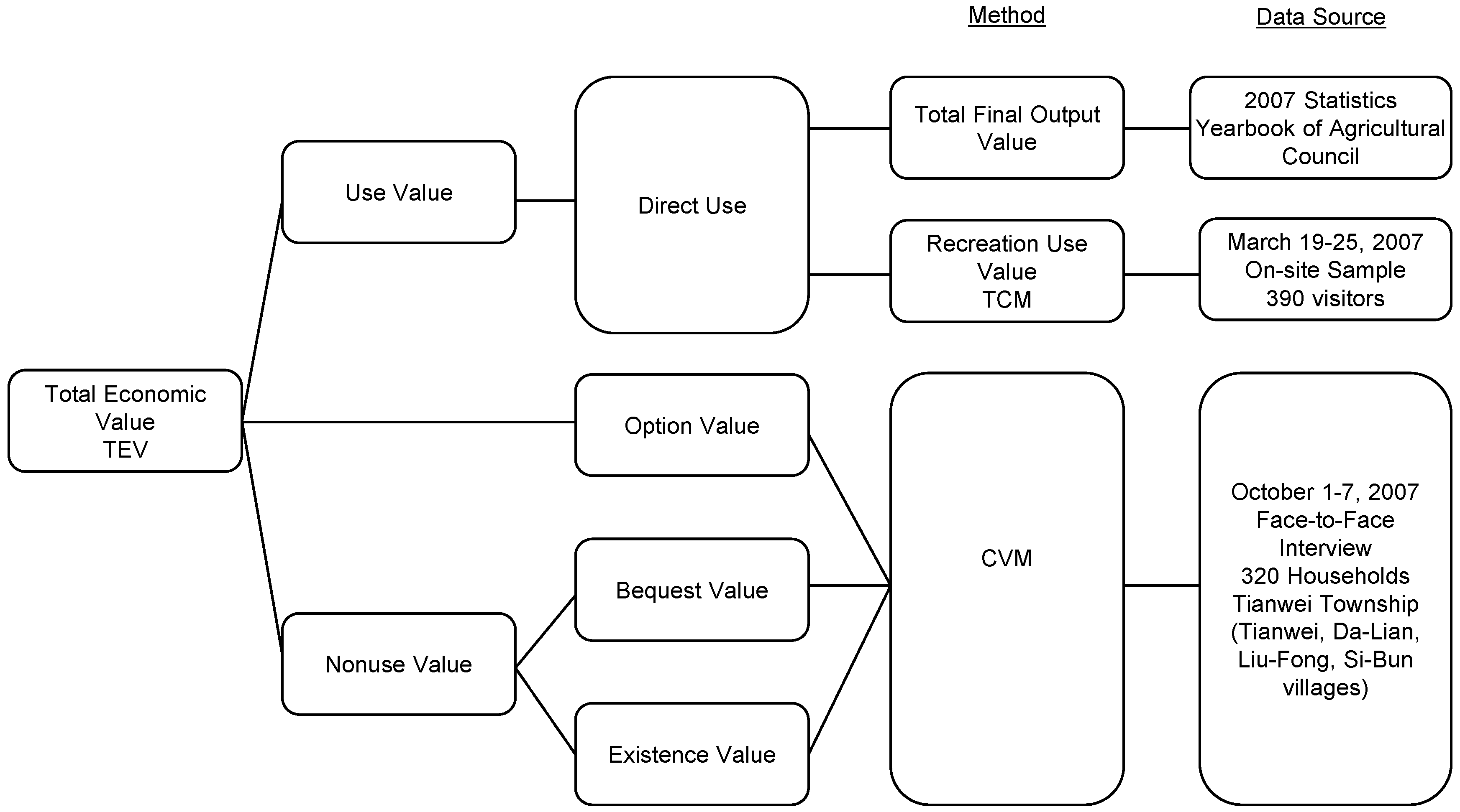
For direct value, the 2007 Statistics Yearbook of the Agricultural Council [65] reports the annual total final flower product value of Tianwei Township. Another direct value is recreational benefits that are collected from Huang et al. (2011) [66]. On-site samples were conducted from 19–25 March 2007 for visitors to Tianwei Highway Garden. Interviews were completed face to face by trained interviewers. During this period, 400 people were asked to complete a questionnaire (Appendix). In total, 390 complete replies were obtained, yielding a response rate of 98%.
For option, bequest, and existence values, the samples were taken from 1–7 October 2007. Tianwei Township contains four main villages (Tianwei, Da-Lian, Liu-Fong, and Si-Bun), and there are 1556 households. During the period, 370 households were interviewed face-to-face with trained interviewers. They were directly asked about their willingness to pay for option, existence, and bequest values. Overall, 320 surveys were completed, yielding a response rate of 86% (Figure 1).
Figure 1. Total economic value and data source.
Sustainability 07 04764 g001
Table 1 lists variable definitions and descriptive statistics. TRIPS, the dependent variable, denotes the number of trips taken by visitors to Tianwei Highway Garden during the past one year. COST denotes total transportation costs, costs incurred on-site, and all opportunity costs. Total round-trip costs and costs incurred on-site were surveyed directly with the respondents. If the respondents could not recall the amount, then round-trip train and bus ticket prices are used. Cost also includes the opportunity cost associated with travel and attendance time, which is calculated by multiplying travel time by one-third of the visitor’s hourly wage. SCOST represents the travel cost associated with a visitor going to a substitute site. This study uses Taichung Lavender Forest as the substitute site. GENDER, MARITAL, and AGE represent respondents’ gender, marital status, and age, respectively. EDU is respondents’ number of education years, and LINCOME represents the log of respondents’ monthly income. HOLIDAY is a dummy variable of visitors who visited Tianwei on a Saturday or Sunday. LIVE is the number of years that residents have lived in their current location. The following are dummy variables: VILLAGE1 (value of 1 if a resident lives in Da-Lian; otherwise 0), VILLAGE2 (value of 1 if a resident lives in Tianwei; otherwise 0), and VILLAGE3 (value of 1 if a resident lives in Liu-Fong; otherwise 0).
Table 1. Variable definitions and descriptive statistics.
VariableDefinitionMeanS.D.
TRIPSNumber of observed trips for individual visits to Tianwei Highway Garden4.826.20
COSTTotal round-trip travel costs to Tianwei Highway Garden (NT dollars)13111301
SCOSTTotal round-trip travel costs to the substitute site, Taichung Lavender Forest17041327
GENDERMale, 1; female, 00.390.49
MARITALMarital status of visitor: married, 1; otherwise, 00.550.50
AGEAge of visitor34.5912.32
EDUEducated years of visitor13.943.14
LINCOMELog of monthly income4.430.22
HOLIDAYDummy, 1, if visitor went to Tianwei Highway Garden on Saturday or Sunday; 0, otherwise0.750.43
LIVENumber of years residents have lived in their current location16.375.38
VILLAGE1Dummy, 1, if a resident lives in Da-Lian; 0, otherwise
VILLAGE2Dummy, 1, if a resident lives in Tianwei; 0, otherwise
VILLAGE3Dummy, 1, if a resident lives in Liu-Fong; 0, otherwise

3. Results and Discussion

3.1. Recreational Benefits

Table 2 lists the estimation result of recreational value from TCM. The log-likelihood ratio tests the model’s goodness-of-fit, which exhibits a Chi-square distribution where the numbers of parameters are associated with the degrees of freedom, demonstrating that the null hypothesis in which all parameters are zero can be rejected at a significance level of 0.01.
The signs of price variables are expected to be consistent with the demand rule for all on-site Poisson models. The coefficients of travel cost and substitute price are negative and significant at the 0.01 level. The analytical results also demonstrate that the coefficients of MARITAL, AGE, EDU, LINCOME, and HOLIDAY are significant in the estimation model. AGE, EDU, and LINCOME are negatively related to the dependent variable, while MARITAL is positively related to the dependent variable—that is, the visitors who are married, younger, and lower educated are more likely to visit Tianwei. The estimation of income elasticity of visitors is −2.19, meaning that visitors with higher income are less likely to visit the recreation site, which is consistent with the definition of an inferior good. This phenomenon may reflect the fact that Tianwei Highway Garden is free for entry.
The consumer surplus is obtained by integrating the demand curve from the initial price to the choke price, which is derived from Equation (5). The average visitor benefit is calculated based on 4.82 trips per year divided by the coefficient of direct cost −0.00058272, which equals NT$8271. The total recreational benefits were roughly NT$17.757 billion for 2.1 million visitors in 2007.
Table 2. Parameter estimates for the travel cost model.
VariableCoefficientt value
INT4.0196(6.662)
COST−0.0006 (−10.1899) ***
SCOST0.0004(8.149) ***
GENDER−0.0369(−0.627)
MARITAL0.4831(6.369) ***
AGE−0.0118(−4.030) ***
EDU−0.0068(−8.9797) ***
LINCOME−0.4223(−3.3361) ***
HOLIDAY0.6037(7.4261) ***
Log likelihood function−15,690
Chi-squared466
Log-likelihood ratio = (−2) × (Restricted Log-likelihood-Log-likelihood), with χ2(8, 0.95) = 15.307. *** p < 0.01, and t values are in parentheses. the actual estimated value is 0.00058272.

3.2. Option, Bequest, and Existence Values

The double-bounded dichotomous choice CVM involves randomly asking tourists about their WTP, as well as a certain pre-chosen price range. Based on the pre-test, this study identifies the top five initial sets of bids: NT$100, 300, 500, 1000, and 2000. The bid is adjusted depending on respondents’ answers, and each individual is asked again about the new amount. If the answer to the first closed-ended question was “yes”, then the sizes of the increases (which in each case represent a rough doubling) given in response to the follow-up question were NT$200, 600, 1000, 2000, and 4000. If the answer to the first close-ended question was “no”, then the sizes of the decreases (which in each case represent a rough halving) stated in response to the follow-up question were NT$50, 150, 250, 500, and 1000. The top five sets of bids in this study are thus: NT$100 (50/200), 300 (150/600), 500 (250/1000), 1000 (500/2000), and 2000 (1000/4000).
The valuation function of a double-bounded model involves dichotomous choice elicitation questions, resulting in interval censoring of individual subject values. As such, the censored survey can use survival analysis to provide a wide parametric distribution. This study follows the conclusions of Stacy (1962) and obtains a family of distributions from the generalized Gamma distribution density function, which is defined as [67]:
f ( E ) = η r ( λ E ) r k 1 exp [ ( η E ) r ] Γ ( k )
Here, η = exp ( α ) denotes the location parameter, r = 1 / σ represents the scale parameter, k = 1 / δ 2 is the shape parameter, and Γ denotes a gamma function. When r = k = 1 (or σ = δ = 1 ), the distribution is exponential. If k = 1 (or δ = 1 ), then the function represents a Weibull distribution. If k (or δ ) is predisposed to infinity, then the lognormal distribution is obtained.
The valuation function employs lognormal, Weibull, gamma, and exponential distributions to explain respondents’ WTP using double-bounded data. Table 3, Table 4 and Table 5 list the complete empirical results, showing that only the Weibull distribution passes the goodness-of-fit test at a 1% significance level for the option, bequest, and existence value models. The scale parameter of the Weibull model differs significantly from 0. Regarding the results, the generalized gamma distribution presents that the Weibull distribution is the best representation of the empirical data.
Table 3. Survival functions to estimate residents’ WTP (willingness to pay) for option value.
VariableLog-normalWeibullGammaExponential
INT1.61 (0.86)3.24 (1.98)2.67 (1.41)2.82 (1.30)
AGE−0.004 (0.46)−0.01 (1.48) *−0.01 (1.08)−0.01 (0.98)
EDU0.01 (0.31)0.02 (0.71)0.02 (0.60)0.02 (0.53)
LNINCOME0.47 (2.39) **0.31 (1.84) *0.37 (1.90) **0.36 (1.60) *
LIVE0.01 (0.98)0.02 (2.48) **0.01 (1.62) *0.01 (1.60) *
VILLAGE10.02 (0.10)0.17 (0.90)0.11 (0.48)0.10 (0.39)
VILLAGE 20.08 (0.39)0.55 (2.87) **0.44 (1.60) *0.43 (1.69) *
VILLAGE 3−0.40 (1.62) *−0.13 (0.62)−0.23 (0.87)−0.23 (0.81)
Scale0.93 (15.76) ***0.73 (14.13) ***0.80 (7.24) ***1 (31.40) ***
Log-likelihood−253.60−252.47−252.23−260.94
Log-likelihood ratio12.03 *25.38 ***14.66 **14.50 **
WTP(NT$)638.48768.08723.14673.06
Log-likelihood ratio = (−2) × (Restricted Log-likelihood-Log-likelihood), χ2(0.95, 7) = 14.05; *, **, and *** mean significance at the levels of 10%, 5%, and 1%, respectively.
Table 4. Survival functions to estimate residents’ WTP for existence value.
VariableLog-normalWeibullGammaExponential
INT1.64 (0.87)3.28 (1.99)2.64 (1.40)2.85 (1.30)
AGE−0.004 (0.48)−0.01 (1.50) *−0.01 (1.07)−0.01 (1.00)
EDU0.01 (0.26)0.02 (0.64)0.02 (0.52)0.02 (0.46)
LNINCOME0.46 (2.36) **0.31 (1.81) *0.37 (1.91) **0.36 (1.58) *
LIVE0.01 (1.07)0.02 (2.57) **0.01 (1.68) *0.01 (1.68) *
VILLAGE10.0004 (0.00)0.15 (0.78)0.42 (1.56) *0.07 (0.27)
VILLAGE 20.08 (0.39)0.56 (2.87) **0.44 (1.60) *0.43 (1.69) *
VILLAGE 3−0.40 (1.62)*−0.13 (0.61)−0.23 (0.91)−0.23 (0.81)
Scale0.92 (15.82) ***0.73 (14.20) ***0.81 (7.95) ***1 (31.52) ***
Log-likelihood−254.31−253.34−252.99−260.94
Log-likelihood ratio10.6123.63 ***13.11 *12.67 *
WTP(NT$)635.02763.75714.40668.61
Log-likelihood ratio = (−2) × (Restricted Log-likelihood-Log-likelihood), χ2(0.95, 7) = 14.05; *, **, and *** mean significance at the levels of 10%, 5%, and 1%, respectively.
Table 5. Survival functions to estimate residents’ WTP for bequest value.
VariableLog-normalWeibullGammaExponential
INT1.70 (0.89)3.42 (2.03)2.57 (1.30)3.03 (1.37)
AGE−0.01 (0.62)−0.01 (1.74) *−0.01 (1.12)−0.01 (1.23)
EDU0.01 (0.19)0.01 (0.47)0.02 (0.37)0.01 (0.32)
LNINCOME0.47 (2.33) **0.31 (1.78) *0.39 (1.94) **0.36 (1.56) *
LIVE0.01 (1.07)0.02 (2.58) **0.01 (1.54) *0.01 (1.72) *
VILLAGE1−0.01 (0.05)0.14 (0.69)0.04 (0.20)0.06 (0.22)
VILLAGE 20.05 (0.21)0.52 (2.63) **0.33 (1.14)0.40 (1.54) *
VILLAGE 3−0.42 (1.69) *−0.17 (0.77)−0.30 (1.13)−0.27 (0.93)
Scale0.93 (15.69) ***0.74 (14.10) ***0.85 (8.18) ***1 (27.60) ***
Log-likelihood−252.95−252.67−252.14−260.40
Log-likelihood ratio13.32 *24.97 ***14.81 **15.56 **
WTP(NT$)636.96767.95702.47676.48
Log-likelihood ratio = (−2) × (Restricted Log-likelihood-Log-likelihood), χ2(0.95, 7) = 14.05; *, **, and *** mean significance at the levels of 10%, 5%, and 1%, respectively.
The coefficient of AGE is negative and significant at the 10% level, which means that residents’ WTP provides option and non-use values that decrease with residents’ age increasing. The coefficient of LNINCOME is positive and also statistically significant at the 10% level, indicating residents with higher income are willing to pay more for option and non-use values. LIVE is positive and significant at the 5% level, showing that the longer residents live their current location, the more WTP they are willing to pay. VILLAGE2 is also positive and significant at the 5% level, which means residents living in Tianwei village clearly have higher WTP than residents elsewhere.
Table 6 summarizes the estimated results of TEV for Tienwei Township. The direct use value of floral products is NT$1.441 billion. The indirect use value, coming from the recreational benefits through floral sightseeing, is NT$17.757 billion by TCM. The option, bequest, and existence values sum up to over NT$15 million by CVM.
Table 6. TEV (Total Economic Value) of Tienwei Township.
WTP/personPopulationTotal Value (NT$ million)
Total Output Value 1441
Recreational ValueNT$8271.002.147 million visitors17,757
Option ValueNT$768.086672 residents5.125
Bequest ValueNT$767.956672 residents5.124
Existence ValueNT$763.756672 residents5.096
The survival valuation function of the Weibull model estimates respondents’ willingness to pay using a median indicator. The advantages of measuring welfare by a median indicator are that it not only eliminates extreme observations, but also has above mean sensitivity to specific distributions [63]. Cooper et al. (2002) compared the confidence interval for the double-bounded model and demonstrated that the mean WTP is more biased than the median WTP with regard to follow-up responses [68]. This study thus adopts the median WTP for valuation, calculated by:
log ( W T P χ ) = X β + σ ε χ , χ = 0.5
The median WTP for option, bequest, and existence values are NT$768.08, 767.95, and 763.75, respectively, as listed in Table 3, Table 4 and Table 5. Based on 6672 village residents, the option, bequest, and existence values are NT$5.125, 5.124, and 5.096 million. The three values may be muddled by respondents who are not familiar with these definitions. The intangible value of Tianwei is likely between NT$ 5 million to NT$15.35 million. The results reveal that the value of farmland is not just production, but also intangible values. Hence, the farmland cannot be simply transferred to residential or business uses based on the low value of agricultural products.
The target of this study is to estimate the true farmland value of Tianwei Township. Omitting these intangible values will underestimate the true economic values of the natural environment, which shall result in incorrect decision-making. Direct use value, which is the total floral output value, was collected from governmental reports. TCM was obtained from visitors, while CVM was acquired from residents. As TCM is a measure of CS and CVM is a measure of WTP, we therefore simply list various estimated results in Table 6.

4. Conclusions

Many farmland areas have been converted to residential or business uses due to the low value of agricultural products. Because agriculture has three functions—production, environmental conservation, and socio-economic—this study argues that recreation use, option, existence, and bequest values will promote farmland value, but their calculations are often omitted in the process of estimating farmland value. Tianwei Township is the largest floral production area in Taiwan and attracts many visitors every year. This study employs TEV to calculate the farmland value of Tianwei Township. Direct use value, which is the total output value of floral products in the region, is obtained from the 2007 Statistics Yearbook of the Agricultural Council [65] in Taiwan, amounting to NT$1.441 billion. Another direct use value, which denotes the recreational benefits through floral sightseeing, is roughly NT$17.757 billion by TCM.
The results of this study demonstrate that recreational benefit is relatively significant, which also shows positive externalities in the forms of recreational amenities and cultural heritage. The aggregation of option, existence, and bequest values in terms of residents may be not large, but these non-rival environment benefits can be enjoyed by millions of people simultaneously in the future. Therefore, the total benefits can be quite significant. Comparing with the wetland system ecosystem study, the amounts of option, existence, and bequest values there are about the same as those in this study. Our results are also similar to the results in the Zander et al. study [22]. Second, the evaluation techniques of this study adopt TCM to estimate recreational benefits and use CVM to evaluate non-use value, which is the same as in Parumog et al. [21] (2003). Third, our valuation methods may provide reliable and useful information to justify specific conservation decisions in this research. Based on Boyd and Banzhaf’s (2007) definition, visitors enjoying beautiful flowers in Tianwei Highway Garden (i.e., recreational benefits) can be considered as “final ecosystem services” [24]. Therefore, to avoid double counting, recreational benefits are generated from visitors, whereas non-use values, and option, bequest, and existence values were collected from residents.
From past experience, once a farmland area in Taiwan is converted to residential or business land area, it becomes a permanent transformation. Therefore, this study recommends to policy makers that agriculture is multifunctional and that sometimes other functions of it could generate more values than just the production function. In their process of decision-making about farmland conversion, they should also consider such factors other than agricultural production.
For policy makers, they can choose to use direct use value or option and non-use values, depending on their tasks. Ignoring the intangible values and environmental externalities leads to an underestimation of the benefits regarding the natural environment. The results of TCM are sensitive to assumptions, including opportunity costs, substitute sites, and the visitors we interviewed. The results of CVM are sensitive to starting point, question setting, and exaggeration bias. Therefore, policy makers should pay extra attention when applying the results from this research. Of course, this study provides the benchmark of the TEV of cultivated flower land. More issues may need to be addressed, such as the productive benefits of biodiversity, fertilizer use upon the environment, and heterogeneous populations with various motives and destinations. These topics could be the focus of further studies. This paper only includes production, environmental conservation, and socio-economic values. Therefore, the limitation is that some other values are not estimated in this study. Further research may adopt the method of Stoeckl et al. (2014) to estimate the value of an ecosystem to avoid double counting the values [69].

Author Contributions

Chin-Huang Huang contributed research design and constructed estimation model. Chin-Huang Huang and Chiung-Hsia Wang jointly analyzed and wrote the paper. All authors read and approved the final manuscript.

Appendix

Questionnaire Example

Tianwei Highway Garden is Taiwan’s most important floral production area. It is a potting whole-sale market. In order to promote tourism, it also serves as an agricultural recreation area. In 2005, 1.1 million visitors came to Tianwei Township, or roughly 3000 visitors daily. Supposing that Tianwei Township wants to conduct sustainable management and invest in infrastructure of Tianwei Highway Garden, what is the maximum amount you would like to pay to maintain the following values?
  • Option Value: A measure to conserve Tianwei Highway Garden, which would allow you to visit or not to visit for an activity in the future.
  • Existence Value: Knowing Tianwei Highway Garden through the news or other resources, you are glad that Tianwei Highway Garden exists and allows you or others to visit it.
  • Bequest Value: The value that you would like to attribute to Tianwei Highway Garden for future generations.
To maintain the three values above, Tianwei Highway Garden association charges you a certain amount of money for visiting (or sells you an entrance ticket). How much would you like to pay for each value? This is a hypothetical questionnaire, and we will not collect any fee from you according to this. The results are for policy evaluation only.
(1)
Would you like to pay NT$500 to maintain the option value of Tianwei Highway Garden?
Yes; would you like to pay NT$1000 to maintain the option value of Tianwei Highway Garden?
No; would you like to pay NT$250 to maintain the option value of Tianwei Highway Garden?
(2)
Would you like to pay NT$100 to maintain the existence value of Tianwei Highway Garden?
Yes; would you like to pay NT$200 to maintain the option value of Tianwei Highway Garden?
No; would you like to pay NT$50 to maintain the option value of Tianwei Highway Garden?
(3)
Would you like to pay NT$300 to maintain the bequest value of Tianwei Highway Garden?
Yes; would you like to pay NT$600 to maintain the option value of Tianwei Highway Garden?
No; would you like to pay NT$150 to maintain the option value of Tianwei Highway Garden?

Conflicts of Interest

The authors declare no conflict of interest.

References

  1. Romstad, E.; Vatn, A.; RøStad, P.K.; Søyland, V. Multifunctional Agriculture: Implications for Policy Design; Report No. 21; Department of Economics and Social Sciences, Agricultural University of Norway: Akershus, Norway, 2000; ISSN 0802-9210. [Google Scholar]
  2. Organization for Economic Co-operation and Developmen (OECD). Multifunctionality: Towards an Analytical Framework; OECD: Paris, France, 2001. [Google Scholar]
  3. European Commission (EC). Safeguarding the Multifunctional Role of Agriculture: Which Instruments? EC: Brussels, Belgium, 1999. [Google Scholar]
  4. Miškolci, S. Multifunctional agriculture: Evaluation of non-production benefits using the analytical hierarchy process. Agric. Econ. 2008, 54, 322–332. [Google Scholar]
  5. Randall, A.; Stoll, J. Existence values in a total valuation framework. In Managing Air Quality and Scenic Resources at National Parks and Wilderness Areas; Row, R.D., Chestnut, L.G., Eds.; Westview Press: Boulder, CO, USA, 1983. [Google Scholar]
  6. Peterson, G.L.; Sorg, C.F. Toward the Measurement of Total Economic Value; USDA Forest Service, Rocky Mountain Forest and Range Experiment Station: Fort Collins, CO, USA, 1987. [Google Scholar]
  7. Pearce, D.W.; Turner, R.K. Economics of Natural Resources and the Environment; Harvester Wheatsheaf: London, UK, 1990. [Google Scholar]
  8. Pearce, D.W. Economic Values and the Natural World; Earthscan: London, UK, 1993. [Google Scholar]
  9. Freeman, M.A. The Measurement of Environmental and Resource Values: Theory and Methods; Resources for the Future: Washington, DC, USA, 1993. [Google Scholar]
  10. Whitehead, J.C. Total economic values for coastal and marine wildlife: Specification, validity, and valuation issues. Mar. Resour. Econ. 1993, 8, 119–132. [Google Scholar]
  11. Bateman, I.J.; Langford, I.H. Non-users’ willingness to pay for a national park: an application and critique of the contingent valuation method. Reg. Stud. 1997, 31, 571–582. [Google Scholar] [CrossRef]
  12. Krutilla, J.V. Conservation reconsidered. Am. Econ. Rev. 1967, 57, 777–786. [Google Scholar]
  13. Pearce, D.W.; Moran, D. The Economic Value of Biodiversity; Earthscan Publication Ltd.: London, UK, 1994. [Google Scholar]
  14. Lazo, J.K.; McClelland, G.H.; Schulze, W.D. Economic theory and psychology of non-use values. Land Econ. 1997, 73, 358–371. [Google Scholar] [CrossRef]
  15. Weisbrod, B.A. Collective-consumption services of individual-consumption goods. Q. J. Econ. 1964, 78, 471–478. [Google Scholar] [CrossRef]
  16. Lee, C.-K.; Han, S.-Y. Estimating the use and preservation values of national parks’ tourism resources using a contingent valuation method. Tourism Manag. 2002, 23, 531–540. [Google Scholar] [CrossRef]
  17. Olsen, G. Option value. Aus. J. Agric. Econ. 1975, 19, 197–209. [Google Scholar]
  18. Togridou, A.; Hovardas, T.; Pantis, J.D. Determinants of visitors’ willingness to pay for the National Marine Park of Zakynthos, Greece. Ecol. Econ. 2006, 60, 308–319. [Google Scholar] [CrossRef]
  19. Plottu, E.; Plottu, B. The concept of total economic value of environment: A reconsideration within a hierarchical rationality. Ecol. Econ. 2007, 61, 52–61. [Google Scholar] [CrossRef]
  20. Loomis, J.; Kent, P.; Strange, L.; Fausch, K.; Covich, A. Measuring the total economic value of restoring ecosystem services in an impaired river basin: Results from a contingent valuation survey. Ecol. Econ. 2000, 33, 103–117. [Google Scholar] [CrossRef]
  21. Parumog, G.M.; Cal, C.P.; Mizokami, S. Using travel cost and contingent valuation methodologies in valuing externalities of urban road development: An application in valuing damages to cultural heritage. J. Eastern Asia Soc. Transp. Stud. 2003, 5, 2948–2961. [Google Scholar]
  22. Zander, K.K.; Signorello, G.; de Salvo, M.; Fandini, G.; Drucker, A.G. Assessing the total economic value of threatened livestock breeds in Italy: Implications for conservation policy. Ecol. Econ. 2013, 93, 219–229. [Google Scholar] [CrossRef]
  23. Yang, W.; Chang, J.; Xu, B.; Peng, C.; Ge, Y. Ecosystem service value assessment for constructed wetlands: A case study in Hangzhou, China. Ecol. Econ. 2008, 68, 116–125. [Google Scholar] [CrossRef]
  24. Boyd, J.; Banzhaf, S. What are Ecosystem Services? The Need for Standardized Environmental Accounting Units. Ecol. Econ. 2007, 63, 616–626. [Google Scholar] [CrossRef]
  25. Pruckner, J.G. Agricultural landscape cultivation in Austria: An application of CVM. Eur. Agric. Econ. 1995, 22, 173–190. [Google Scholar]
  26. Poor, P.J.; Smith, J.M. Travel cost analysis of a cultural heritage site: the case of historic St. Mary’s city of Maryland. J. Cult. Econ. 2004, 28, 217–229. [Google Scholar] [CrossRef]
  27. Yung, E.H.K.; Yu, P.L.H.; Chan, E.H.W. Economic Valuation of Historic Properties: Review and Recent Developments. Prop. Manag. 2013, 31, 335–358. [Google Scholar]
  28. Loomis, J.B.; Walsh, R.G. Recreation Economic Decisions: Comparing Benefits and Costs; Venture Publishing, Inc.: Edmonton, AB, Canada, 1997. [Google Scholar]
  29. Fix, P.; Loomis, J. Comparison the Economics Value of Mountain Biking Estimated Using Revealed and Stated Preference. J. Environ. Plan. Manag. 1998, 41, 227–236. [Google Scholar] [CrossRef]
  30. Siderelis, C.; Moore, R. Outdoor recreation net benefits of rail-trails. J. Leisure Res. 1995, 27, 344–359. [Google Scholar]
  31. Carson, R.T.; Flores, E.N.; Martin, M.K.; Wright, L.J. Contingent Valuation and Revealed Preference Methodologies: Comparing the estimates for qusi-public goods. Land Econ. 1996, 72, 80–89. [Google Scholar] [CrossRef]
  32. Common, M.; Bull, T.; Stoeckl, N. The travel cost method: An empirical investigation of Randall’s Difficulty. Aust. J. Agric. Resource Econ. 1999, 43, 457–477. [Google Scholar] [CrossRef]
  33. Randall, A.A. Difficulty with the travel cost method. Land Econ. 1994, 70, 88–96. [Google Scholar] [CrossRef]
  34. Bockstael, N.E.; Strand, I.E.; Hanemann, W.M. Time and the recreational demand model. Am. J. Agric. Econ. 1987, 69, 293–302. [Google Scholar] [CrossRef]
  35. U.S. Water Resources Council. Economic and Environmental Principles and Guidelines for Water and Related Land Resources Implementation Studies; U.S. Government Printing Office: Washington, DC, USA, 1983.
  36. McConnell, K.E.; Strand, I. Measuring the cost of time in recreational demand analysis: An application to sport fishing. Am. J. Agric. Econ. 1981, 63, 153–156. [Google Scholar] [CrossRef]
  37. Rosenthal, D.H. The necessity for substitute prices in recreation demand analysis. Am. J. Agric. Econ. 1987, 69, 828–837. [Google Scholar] [CrossRef]
  38. Chakraborty, K.; Keith, J.E. Estimating the recreation demand and economic value of mountain biking in Moab, Utah: An application of count data models. J. Environ. Plan. Manag. 2000, 43, 461–469. [Google Scholar] [CrossRef]
  39. Hellerstein, D.; Mendelsohn, R. A theoretical foundation for count data models. Am. J. Agric. Econ. 1993, 75, 604–611. [Google Scholar] [CrossRef] [Green Version]
  40. Creel, M.D.; Loomis, J.B. Theory and empirical advantages of truncated count data estimators for analysis of deer hunting in California. Am. J. Agric. Econ. 1990, 72, 434–441. [Google Scholar] [CrossRef]
  41. Shaw, D. On-site samples’ regression: Problem of non-negative integers, truncation and endogenous stratification. J. Econ. 1988, 37, 211–223. [Google Scholar] [CrossRef]
  42. Englin, J.; Shonkwiler, J.S. Estimating social welfare using count data models: An application to long-run recreation demand under conditions of endogenous stratification and truncation. Rev. Econ. Stat. 1995, 77, 104–112. [Google Scholar] [CrossRef]
  43. Englin, J.; Shonkwiler, J.S. Modeling recreation demand in the presence of unobservable travel costs: Toward a travel price model. J. Environ. Econ. Manag. 1995, 29, 368–377. [Google Scholar] [CrossRef]
  44. Grogger, J.T.; Carson, R.T. Models for truncated counts. J. Appl. Econ. 1991, 6, 225–238. [Google Scholar] [CrossRef]
  45. Bishop, R.C.; Heberlein, T.A. Measuring values of extramarket foods: Are indirect measures biased? Am. J. Agric. Econ. 1979, 61, 926–930. [Google Scholar] [CrossRef]
  46. Mitchell, R.C.; Carson, R.T. Using Surveys to Value Public Goods: The Contingent Valuation Method; Resource for the Future: Washington, DC, USA, 1989. [Google Scholar]
  47. Cameron, T.A.; James, M.D. Efficient Estimation Methods for Closed Ended Contingent Valuation Survey. Rev. Econ. Stat. 1987, 69, 269–276. [Google Scholar] [CrossRef]
  48. Cummings, R.G.; Brookshire, D.S.; Schulze, W.D. Valuing Environmental Goods: A State of the Arts Assessment of the Contingent Valuation Method; Roweman and Allanheld: Totowa, NJ, USA, 1986. [Google Scholar]
  49. Veronesi, M.; Alberini, A.; Cooper, J.C. Implication of bid design and willingness-to-pay distribution for starting point bias in double-bounded dichotomous choice contingent valuation surveys. Environ. Resour. Econ. 2011, 49, 199–215. [Google Scholar] [CrossRef]
  50. Haab, T.C.; McConnell, K.E. Valuing Environmental and Natural Resources; Edward Elgar Publishing, Inc.: Cheltenham, UK, 2002. [Google Scholar]
  51. Walsh, R.G.; Loomis, J.B.; Gillman, R.A. Valuing option, existence and bequest demands for wilderness. Land Econ. 1984, 60, 14–29. [Google Scholar] [CrossRef]
  52. Kanninen, B.J. Bias in discrete response contingent valuation. J. Environ. Econ. Manag. 1995, 28, 114–125. [Google Scholar] [CrossRef]
  53. Park, J.H.; MacLachlan, D.L. Estimating willingness to pay with exaggeration bias-corrected contingent valuation method. Mark. Sci. 2008, 27, 691–698. [Google Scholar] [CrossRef]
  54. Johannesson, M.; Liljas, B.; Johansson, P.O. An experimental comparison of dichotomous choice contingent valuation question and real purchase decisions. Appl. Econ. 1998, 30, 643–647. [Google Scholar] [CrossRef]
  55. Lee, W.S.; Graefe, A.R.; Hwang, D. Willingness to pay for an ecological park experience. Asia Pac. J. Tour. Res. 2012, 18, 288–302. [Google Scholar] [CrossRef]
  56. Scarpa, R.; Bateman, I. Efficiency gains afforded by improved bid design versus follow-up valuation questions in discrete-choice CV studies. Land Econ. 2000, 76, 299–311. [Google Scholar] [CrossRef]
  57. Alberini, A. Efficiency vs. bias of willingness to pay estimates: Bivariate and interval-data models. J. Environ. Econ. Manag. 1995, 29, 169–180. [Google Scholar] [CrossRef]
  58. Hanemann, W.M.; Loomis, J.; Kanninen, B. Statistical efficiency of double-bounded dichotomous choice contingent valuation. Am. J. Agric. Econ. 1991, 73, 1255–1263. [Google Scholar] [CrossRef]
  59. Carson, R.D.; Wilks, L.; Imber, D. Valuing the preservation of Australia’s Kakadu Conservation Zone. Oxf. Econ. Pap. 1994, 46, 727–749. [Google Scholar]
  60. Bateman, I.J.; Langford, I.H.; Jones, A.P.; Kerr, G.N. Bound and path effects in double and triple bounded dichotomous choice contingent valuation. Resour. Energy Econ. 2001, 23, 191–213. [Google Scholar] [CrossRef]
  61. Kerr, G.N. Dichotomous choice contingent valuation probability distributions. Aus. J. Agric. Resour. Econ. 2000, 44, 233–252. [Google Scholar] [CrossRef]
  62. Imber, D.; Stevenson, G.; Wilks, L. A Contingent Valuation Survey of the Kakadu Conservation Zone; Research Paper No. 3; Resource Assessment Commission, Commonwealth Government Printer: Canberra, Australia, 1991.
  63. Nelson, W. Applied Life Data Analysis; John Wiley: New York, NY, USA, 1982. [Google Scholar]
  64. León, C.J. Double bounded survival values for preserving the landscape of natural parks. J. Environ. Manag. 1996, 46, 103–118. [Google Scholar] [CrossRef]
  65. Council of Agriculture. Agricultural Statistics Yearbook; Council of Agriculture: Taipei, Taiwan, 2007.
  66. Huang, C.H.; Huang, Y.H.; Lin, W.L.; Hsiao, P.H. Estimating recreational benefits and environmental effects for the amenities of flowers industry. Adv. Manag. 2011, 4, 60–65. [Google Scholar]
  67. Stacy, E.W. A generalization of the Gamma distribution. Ann. Math. Stat. 1962, 33, 1187–1192. [Google Scholar] [CrossRef]
  68. Cooper, J.C.; Hanemann, M.; Signorello, G. One-and-one-half-bound Dichotomous Choice Contingent Valuation. Rev. Econ. Stat. 2002, 84, 742–750. [Google Scholar] [CrossRef] [Green Version]
  69. Stoeckl, N.; Farr, N.; Larson, S.; Adams, V.M.; Kubiszewski, I.; Esparon, M.; Costanza, R. A new approach to the pfoblem of overlapping values: A case study in Australia’s Great Barrier Reef. Ecosyst. Serv. 2014, 10, 61–78. [Google Scholar] [CrossRef]

