Article

Determinants and Sustainability of House Prices: The Case of Shanghai, China

1
Faculty of Tourism and Industrial Development, Chengdu University, Chengdu 610106, China
2
The Ronald Coase Centre for Property Rights Research, Faculty of Architecture, The University of Hong Kong, Hong Kong, China
*
Author to whom correspondence should be addressed.
Sustainability 2015, 7(4), 4524-4548; https://doi.org/10.3390/su7044524
Submission received: 11 February 2015 / Revised: 29 March 2015 / Accepted: 9 April 2015 / Published: 16 April 2015
(This article belongs to the Section Economic and Business Aspects of Sustainability)

Abstract

:
Recent housing policies include measures for home purchase control and shanty town redevelopment. This study proposes sustainable pricing, in that the long-run equilibrium price is determined by the fundamentals of house prices. We argue that changes in CPI might have led to rapidly growing house prices and rather high price levels. We investigate the long-run or short-run impacts of new commodity housing completions, transacted square meters of commodity housing, and CPI for house prices in Shanghai. We adopt monthly data for the period of 2005–2010. We test for unit roots using both the ADF and PP techniques and structural breaks using both the Zivot-Andrews (Model B) and Perron (Model C) methods. Considering Cheung-Lai and Reinsel–Ahn finite-sample corrections, the results suggest a long-run equilibrium. Housing completions negatively impact house prices in the short run. A positive volume-price relationship is suggested. Housing sales affect house prices in the short run but not vice versa. Hence, the empirical evidence supports the search model. In addition, CPI is strongly exogenous with respect to the long-run relationship and thus is a long-term determinant of house prices. CPI also positively and drastically influences house prices in the short run. Therefore, a reduction in inflation rate could stabilize house prices, increasing the chances of sustainable prices in the future.

1. Introduction

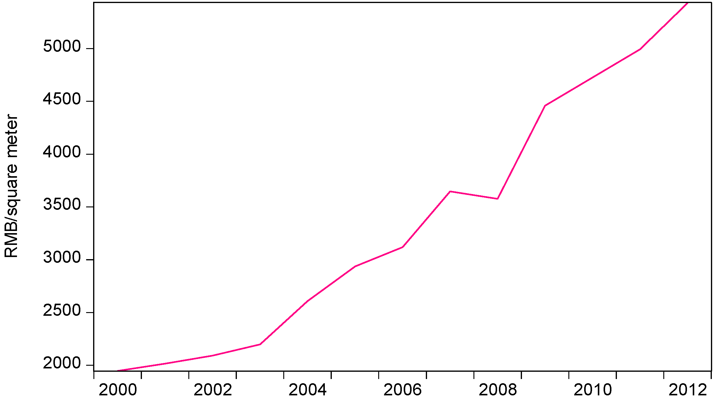
In 2000–2008, the average house price in Chinese cities increased by 84% (Figure 1) [1]. In Shanghai, during 2001−2008, the prices of new commodity and existing housing properties grew by 76.7% and 88.5%. More recently, in 2006−2008, these prices rose by 9.3% and 10.9% (Table 1) [2]. This may suggest a house price bubble in Shanghai, e.g., [3]. House price levels have significantly increased given the high ratio of house price to family income [4]. Moreover, an influx of overseas funds has resulted in a real estate market boom in Shanghai [5]. Additional factors significantly influencing the changes in house prices are real estate investment, per capita disposable income, and employment opportunities [6]. Also, urban rapid transit has a significant incremental impact on the prices of houses located near transport stations [7].
Figure 1. Average urban commodity housing price in China.
Sustainability 07 04524 g001
Table 1. Housing completions, sales, and prices in Shanghai.
Items20012002200320042005200620072008200920102013
Sale prices of new commodity housing properties102.1 111.0 134.7 156.0 170.4 165.0 170.6 180.4 ---
Sale prices of existing housing properties110.8 117.1 142.4 167.3 185.1 188.4 195.6 208.9 ---
Housing land transaction prices92.2 102.3 125.1 161.8 170.6 169.7 177.2 189.5 ---
Sales of new commodity housing properties (10,000 m2)1647.91839.12224.53233.72845.72615.493279.21965.92928.0--
Completed new commodity housing properties (10,000 m2)1501.91708.02139.93076.22739.92699.12752.51763.31508.81396.051609.13
Notes: Prices are measured in indices (2000 = 100).
The Chinese government has implemented both demand- and supply-side housing policies that aim to restrain the excessive growth of house prices. The 2010 home purchase policy exerts control over the amount of commodity housing purchased for a family [8]. However, average house prices in Chinese cities went on to increase by 52% during 2008–2012 [1]. In Shanghai, commodity housing rent increased by 13.6% during 2005–2008 and18.7% between 2008 and 2012 [9]. Local governments often misallocate security housing properties to high- or relatively high-income families [10,11,12]. Land hoarding and idle urban land plots could result in a shortage in housing supply [13,14]. Hence, China expects to increase residential supply by redeveloping shanty towns on a large scale from 2013 to 2017 [15].
Housing economics suggests that housing supply and housing demand interact. The demand-supply interactions determine house prices. Housing supply, housing demand, and price tend to adjust to the long-run equilibrium [16,17,18,19]. In a housing market, both consumers’ and sellers’ price expectations are backward-looking [20], and thus a demand shock will not instantaneously influence the level of list prices [21]. The seller and buyer are able to carry out a transaction mostly based on the price change in the preceding period. Sellers and buyers not only can instantly obtain but also readily understand the information on the number or square meters of housing sales. However, housing markets are informationally imperfect and asymmetric. Housing estates are heterogeneous; hence, the general public cannot instantly obtain data on the price level or index price change. Instead, housing market participants usually utilize sales information to forecast the price change. In other words, changes in sales would lead changes in prices.
The search model assumes that sales are weakly exogenous to house prices. It has been suggested that sales Granger-cause prices [22]. Demand shock is weakly exogenous both to sales and house prices [21,23]. Consequently, sales respond more quickly than prices to a shock in demand. Since the increase (decrease) in sales in the preceding period predicts the market boom (bust), a positive volume-price relationship is proposed and has received increasing empirical support [22,23,24,25]. Also, due to house price dispersion, an increase in volume (liquidity) reduces the required risk premium in buyers’ offering prices and thus tends to raise their reservation prices [26].
The housing market in Shanghai is typically characterized by a rather high ratio of new housing estate sales to total housing sales. Transactions of new commodity housing properties have accounted for a substantial share of the total housing sales. In 2005, completed housing properties (27.4 million square meters) accounted for 96.3% of the sales of commodity housing properties (28.46 million square meters). By 2010, the share of completed housing properties (13.96 million square meters) in the sales of commodity housing properties (16.85 million square meters) was still as high as 82.8% [2]. The change in housing completions may be measured as a housing supply variable. Housing supply significantly affects house prices [10,11,27,28]. Hence, we can expect that the change in housing completions affects the change in prices.
However, the consumer price index (CPI) may be a determinant of the rapidly escalating house prices. In fact, monetarist theory indicates that excessive money supply leads to price inflation [29,30]. A higher expected rate of inflation tends to increase the real after-tax rate of return on owner-occupied housing relative to that on other assets with a similar risk, thus tending to raise its equilibrium price [31]. Higher anticipated inflation rates result in higher house prices as households increase their demand for housing assets during inflationary periods [32]. Money shocks have exerted short-run dynamics on both actual house prices and housing sales (new starts and existing homes) [33]. A nearly 350-year house price index shows that, excluding inflation, house price has experienced little structural increase; specifically, the real price in 1973 was only twice as high as it was in 1628 [34]. Hence, real estate is the best hedge against expected and unexpected inflation [32,35,36]; house prices are simply an inflation hedge in the long run [37,38].
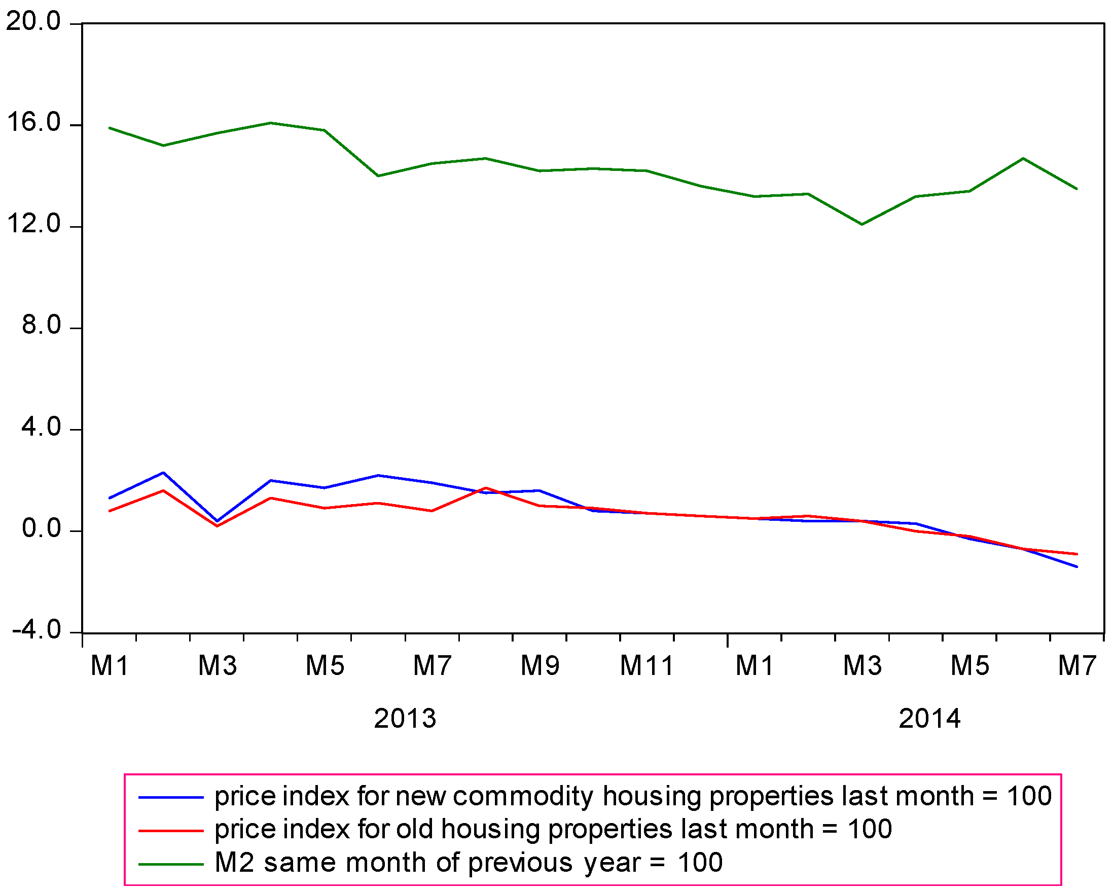
Figure 2 shows that house prices appear to change with broad money (M2). In 2003, China’s M2 supply and house prices grew by 19.6% and 5.7% compared with the same period of previous year. In 2008, these two macroeconomic indicators recorded a growth of 17.8% and 7.1%. Mortgage in China is incredibly vast. Home loans amounted to RMB 9 trillion at the end of 2013, accounting for 11.7% of the total loan balance and 8.1% of M2 balance [39]. Furthermore, in Shanghai, personal housing loans accounted for 90.9% in 2010 and 77.7% in 2012 of the consumer credit [9]. Hence, excessive money supply might have increased house prices [40]. Moreover, in 2012, approximately 4300 million square meters of urban commodity housing was still under construction. Thus, concerned about the massive stock of new homes remaining unsold, in October 2014, the central government advised banks to provide preferential loans for the purchases of homes in cities [41].
Figure 2. Changes (%) in national city house prices and M2, China (data source: [42,43]).
Sustainability 07 04524 g002
Figure 3. Changes (%) in house prices and M2, Shanghai (data source: [42,43]).
Sustainability 07 04524 g003
Therefore, it seems that the home purchase policy has not restrained the fast-growing house prices. The issue is whether CPI impacts house prices. It is noteworthy that since June 2013, China has been implementing a prudent monetary policy [15]. With the moderate money supply expected to continue [44], M2 supply has been gradually decreasing. Meanwhile, house prices in Shanghai appear to be declining with the money supply (Figure 3).
Therefore, suppose that there is a four-variable system containing house prices (HOUSE PRICE), housing completions (COMPLETION), sales volume (SALES), and inflation rate (CPI):
( H O U S E P R I C E , C O M P L E T I O N , S A L E S , C P I )
In this system, the change in CPI would distort the change in prices determined by demand and supply variables. As shown above, both sales and CPI are expected to be exogenous to the price.
This paper aims to investigate the determinants of house prices in Shanghai. Empirical evidence will help differentiate between the impacts of housing completions, trading volume, and CPI on house prices. We also present the housing policy evolution for the period 2006–2013. The remainder of this article is organized as follows. Section 2 suggests the sustainable house price. Section 3 reviews variations in the housing policy. Section 4 describes the econometric methods and data and defines the variables. Section 5 presents the econometric results and discusses few of them. Section 6 concludes the study.

2. Sustainable House Prices

In this study, we argue that sustainable house price in that the price varies smoothly in the long run. At such a price, housing properties are affordable to people with a median household income, as rated by a country, region, or city. The previous study justifies the existence of a unique sustainable price vector for a multiproduct firm. A sustainable price is the average cost price [45]. In addition, the sufficiently large size of the firm can lead to a sustainable monopoly price [46].
Therefore, a sustainable price can be the long-run equilibrium price. An equilibrium price is determined by macro fundamentals. The fundamentals of house prices include economic output, demographic factors and land [47], foreign investment [48], housing supply and demand [18,19,23,49,50], real estate returns [51], and inflation rates [31,32,37,38].
Inflation usually undermines the equilibrium house price, thereby resulting in a price bubble. In 1950–1973, inflation produced a significant increase in the nominal home price as compared to its long-run stable variations (during 1628–1973). However, the appreciation of the real home price almost disappeared in the long term [34].
A price bubble would build if fundamental factors did not justify such a price [52], and an increasingly large price bubble will eventually burst. Such a price is not sustainable in terms of growth rate and level. A striking decrease in economic growth rates can largely account for the collapse of urban land prices in Japan after the mid-1990s [53]. Price bubbles can be easily represented by an error-correction model (ECM) [54,55,56]. The first-differenced and one-time lagged ECM that models the performance of home price movements in [56] can be written as
Δ P t = α + β 1 Δ P t - 1 + β 2 Δ i n t e r e s t r a t e t + β 3 Δ u s e r c o s t t + β 4 Δ C P I t + δ ( ln P t _ 1 * - ln P )
where P* is the equilibrium house price. Mortgage rate, housing user cost, and inflation rate represent few fundamentals of house prices. β1 is a bubble builder and δ a “bubble burster”. For example, β1 and δ for home prices in three New Zealand cities are 0.4 and 1.2, suggesting that the price bubble exists but it is not nearly a burster [54].
ECM holds because time series variables are cointegrated [57,58,59]. Under the circumstances of cointegration, house prices move around a long-run equilibrium vector. Cointegration can be a sufficient condition for long-run price sustainability. A necessary condition is that in the cointegrating system, other variables such as trading volume and CPI influence prices. In other words, completions, trading volume, and/or CPI may be weakly or strongly exogenous with respect to the cointegrating system [60].

3. Review of Housing Demand and Price Policies in 2005−2013

This section elucidates that the housing policy aimed to restrain investment and speculative demand for housing properties since early 2010. A general review of the urban housing policies during 1998−2007 has been presented [61]. The policy excluded regulations regarding the containment of investment and speculative demand for housing properties during 2006−2009. In addition, the policy was designed only to curb the excessive escalation of house prices during June 2006−2010, which can explain the swift escalation of house prices in Chinese cities over the past few years.

3.1. The Demand Policy Omitted the Containment of Investment and Speculative Demand for Housing Properties in 2006−2009; the Policy Potentially Stimulated the Swift Growth in Investment Demand and Could Be the Reason for the Rapid Escalation of House Prices

For approximately four years, the central government’s housing policy excluded the regulation restraining investment and speculative demand for housing properties, although this containment had been emphasized as early as 2005 [62,63]. Therefore, we inferred that the housing policy during this period could potentially stimulate the investment demand for housing properties. The easy lending policy and delays in property tax trials over the past few years can justify this. The government imposed few limits on mortgage loans for investment or speculative home purchases from 2005 to mid-2010. In particular, during the 2008–2009 global financial crisis, the lending policy supported the purchases of upgraded housing properties and provided tax preferences for the transactions of these properties [64,65]. Property taxes may negatively influence house values or prices by restraining housing demand [66,67,68]. The central government promised to steadily formulate property tax reforms and trials in as early as 2006, which was the first year of the 11th Five-Year Economic Plan period (2006−2010) [69]. China did not launch a property tax trial in any city at the end of 2010. Therefore, the exclusion of the provision to restrain investment and speculative housing demand may have encouraged such demand.
The pillar status of the real estate industry in China may account for the exclusion of the regulation to restrain investment and speculative housing demand from relevant documents. The central government has been describing the real estate industry as a pillar industry since 2003 [62,70]. However, in 2008, the central government adopted a vague attitude regarding this pillar status and has not specified the pillar status of the industry ever since. On the other hand, it did not explicitly remove the real estate sector from the listed pillar industries [64,71,72]. Moreover, it is noteworthy that the list of planned and selected top ten promotion industries does not include the real estate industry [73].
However, a shortage in the supply of housing resources can lead to not only the rapid escalation of house prices but also price levels that are higher than local family disposable incomes. The short supply of security housing resources [10,11] also leads to higher house price levels [11]. Housing security in China is said to have limited coverage. The authorities often misallocate security housing properties to high- or relatively high-income families, resulting in an apparent lack of fairness in the housing security system [12]. In addition, land hoarding and idle urban land idle can be mainly attributed to the shortage of land supply for housing asset construction, and accordingly, to a shortage in housing supply. The law stipulates that a developer must begin real estate activities on a plot within two years of acquiring the plot from the city government. Otherwise, the government can rescind the right of using this plot from the developer [72]. However, a large number of developers in China have hoarded vacant lands without any development for natural gains in the future. This can be attributed to China’s rapid urbanization since the 1990s. In theory, the expanding population and economic size of a city lead to the appreciation of land values; therefore, numerous idle plots are being hoarded by developers, which are exacerbating the problem of the shortage of land supply in the markets for the development of housing properties. China’s Ministry of Land and Resources (MLR) found that over 70% of the 9772 hectares of land left idle by real estate development companies have been designated for housing uses [13]. In addition, by the end of May 2010, 3070 plots nationwide were reported to the MLR for violating the law. Approximately 31% of the plots reported had been left idle for five years or more [14].

3.2. The Price Policy Aimed at Curbing the Excessive Escalation of House Prices in June 2006−2010, Thereby Leading to Expectations of Rapid Escalation in House Price Levels

In March 2005, the central government assigned the responsibility of stabilizing house prices to the local governments [62]. The use of the neutral words “stable prices” in the policy indicated that the central government believed that house prices could be controlled using macroprudential measures. It has been indicated that the Chinese government has used a macroprudential policy toolkit in order to curb the increase in house prices [74]. However, housing policy for house prices has significantly changed ever since. The policy intended only to restrain the excessive escalation of house prices; therefore, the realization of stable prices was no longer the goal of the policy [63]. As a result, the average house prices in Chinese cities increased by as much as 8.2% in 2005 [75]. Hence, June 2006 was a significant turning point for the macro-control targets for the escalation of house prices. This policy of restraining fast-growing house prices began in June 2006 and continued for three and a half years. In April 2010, the central government continued to direct local governments in taking firm measures to curb the excessive escalation of house prices in individual cities [76]. This indicates that the central government may have recognized an upward trend in the house prices of Chinese cities over a relatively long period. In addition, to deal with the 2008−2009 financial crisis, China needed to stabilize the confidence in the property market and the size of real estate investment [64,65]. The additive effect of these policies may have greatly contributed to the rapid escalation of urban house prices over the past few years. For example, compared to previous year, the average house prices in Chinese cities increased by 5.9%, 8.6%, and 7.4% in 2006, 2007, and 2008, respectively [75].
It is worth noting that since January 2011, the target of housing macro-regulative policy represents the realization of a third significant change over the past five years. The central government formulated a new plan in January 2011. The program requires local governments to undertake effective measures to maintain house prices at reasonable levels. In particular, it is the first instance in which the State Council is required to control targets for home price levels in various cities [72]. The Shanghai municipal government has committed to maintaining the regional house prices at reasonable levels to fulfil the requirements of the central government’s latest prudential housing policy [77]. However, the central government does not elucidate the equitable price level. Nevertheless, a significant change in this new policy is that the State Council deleted the words “restraining excessive escalation of house prices”. Similar words had been regularly used by the central government in a few of its key documents during 2006−2010. Therefore, the central government appears to have not permitted the rapid or relatively quick escalation of house prices in cities, thereby assuming a neutral tendency towards the growth rates of domestic house prices.

3.3. The Policy Encourages Reasonable Demand for Housing Properties; in Particular, the Policy Aimed to Restrain the Investment and Speculative Demand for Housing Properties since Early 2010

A few rather important documents on housing market macroprudential measures encouraged the supply of certain housing resources, including ordinary commodity housing, affordable housing [62,64,78], and public rental housing [65,72,76]. In addition, reasonable housing properties include those that are densely constructed and have small floor areas. The government released a guide for housing development that states that the development area for housing units with a floor area of 90 square meters or below must account for at least 70% of the overall development area of an individual housing neighbourhood. The city government must provide over 70% of the entire city’s land supply for the construction of ordinary housing resources, which mostly comprise low- and medium-priced properties, small- and medium-sized affordable properties, and low-rent rental housing [72,76,78]. Finally, a reasonable demand must be one for self-servicing housing properties [63,79].
Unreasonable housing demand is related to assorted property types. These housing types comprise sparsely developed and high-end properties, villas [62], spacious units, properties of repeated transactions within five years, properties induced by illegal demolitions, and investment and speculative resources. For example, a family (composed of a spouse and their children) in the city may own a home with a floor area of 90 square meters or above. The second home purchased by this family may be for investment [72,76]. However, the central government has increased the minimum down payments of mortgages for the purchases of additional properties to curb investments in housing properties [72,79]. In addition, resale housing properties are those purchased for investment or speculation. Hence, greater income tax is charged on homes that are transacted twice or more in five years [72].

3.4. Housing Policy Enters the Period of Investment Containment and Speculative Demand for Housing Properties (Early 2010–Mid-2013)

The policy states that local governments must (effectively) contain home purchases for the purposes of investment and speculation [71,72,76]. Therefore, all municipalities, provincial cities, and any other city with soaring house prices must release local detailed regulations to limit the number of home purchases. The regulations affect local permanent families as well as local temporary residences [72]. The Shanghai municipal government has suspended home purchases by Shanghai resident families that own two or more apartments and non-Shanghai resident families that own one or more apartments [77]. In addition, the municipalities of Shanghai and Chongqing have launched property tax trials. On 28 January 2011, these two metropolises announced the levying of taxes on a portion of housing assets. The property tax reform was a breakthrough because China lacked a tax system that could be levied on house property holdings. Property tax trials are expected to curb investment in and speculative demand for housing properties, thereby negatively influencing house prices.

3.5. The Significant Changes in Housing Market Fundamentals since Mid-2013 Include Market-Orientated Management, Shanty Town Reconstruction, Establishment of the Property Registry System, and a Prudent Monetary Policy

Market-orientated management implies that a housing policy that heavily depends on demand controls is questionable. Since mid-2013, a growing number of cities have removed home purchase controls [80]. China has aimed to redevelop about 10 million shanty towns between 2013 and 2017. Although urban redevelopment can increase housing supply, it also leads to the growth of short-term demand for housing properties—while the former has a negative effect, the latter has a positive one on housing prices. China will release Rules for Property Registry in late 2014 and have full property information networked before 2017, which will accelerate the levying of personal property tax and reduce the speculative or investment demand for housing properties. In 2013, M2 grew by 13.6% and money supply remained prudent in 2014 and will continue to do so in 2015 [81]; M2 was expected to increase up to 13% in 2014 [15,44]. Therefore, the cancelation of home purchase control has not resulted in the growth of housing sales and prices [82]. We anticipate that market-orientated management and prudent monetary policy will lead to the sustainable growth of house prices.

4. Methods and Data

4.1. Methods

Suppose house prices, housing completions, sales, and inflation rates interact within a unique housing market. Long-run equilibrium forms among these variables. To investigate the possible long-run equilibrium relationship(s) between house prices and potential price determinants, we conducted cointegration tests using the Johansen multivariate trace test [83,84,85]. Cointegration implies a long-run equilibrium relationship between time-series variables. ECM can represent the long-run relationship [86]. Cointegration between house prices and trading volume has been suggested [21,22].
We employed the critical value corrections [87] and trace corrections [88] to control for finite-sample biases. In addition, the residual-based Engle-Granger test provided further evidence for cointegration [57]. The trace analysis is based upon
Δ y t = Π y t - 1 + i = 1 p - 1 Γ i Δ y t - i + B x t + ε t
where Π = i = 1 p A i I and Γ i = j = i + 1 p A j . yt is a k-vector of I(1) variables, xt is a d-vector of deterministic variables, and εt is a vector of white noises with zero mean and finite variance. Furthermore, Π = α β , where β and α are the cointegrating vector and corresponding adjustment coefficient. β represents the long-run relationship between time series.
Cointegration implies the existence of a (reduced-form) ECM:
Δ y t = λ + k = 1 m π k Δ y t - k + k = 1 m ξ k Δ x t - k + δ z t - 1 + ε t
where yt and xt are I(1) time-series variables. zt − 1 is the error correction (EC) variable representing a long-run equilibrium. A single cointegrating relationship between four variables can be written as z t - 1 = ( y t - 1 - β 1 x 1 t - 1 β 2 x 2 t - 1 - β 3 x 3 t - 1 - μ ) , where β1, β2, and β3 are the long-run elasticities of y with respect to x. Super-consistency of cointegration [89] allows us to incorporate the cointegrating vector β obtained by the Johansen tests into the ECM as an EC term. Coefficient δ is the proportion of the last period’s short-run disequilibria from long-run equilibrium modified in the next period. Hence, δ is called the adjustment coefficient. If changes in Δ y t are above its long-run equilibrium (average) value, the EC term is positive. In this case, Δ y t must move downwards to return to the long-run equilibrium path. Thus, δ is expected to be negative.
To increase the robustness of unit root tests, we conducted both the augmented Dickey-Fuller (ADF) test [90,91] and the Phillips-Perron (PP) test [92]. Most macroeconomic series are I(1) [93]. However, the presence of a break date in the series may lead to a spurious unit root [94]. Hence, we conducted structural break tests using the Perron (Model C) and the Zivot-Andrews (Model B) tests [95,96]. The Perron test rejects the null hypothesis of a unit root more frequently than the Zivot-Andrews test. The mixed Model C for the break date test is [94]
y t = μ + θ D U t + β t + γ D T t + d D ( T B ) t + α y t - 1 + i = 1 k Δ y t - i + ε t
Model C (the mixed model) allows for a one-time change in the level and a change in the slope of the trend function. Removing the dummy variable D(TB) from Equation (5), we obtain Model B (the changing growth model):
y t = μ + θ D U t + β t + γ D T t + α y t - 1 + i = 1 k Δ y t - i + ε t
Under the hypothesis of a unit root, μ ≠ 0 (in general), β = 0, θ = 0 (except in Model C), γ = 0, d ≠ 0, and α = 1. Under the alternative hypothesis of stationary fluctuations around a deterministic trend function, μ ≠ 0, β ≠ 0, θ ≠ 0, γ ≠ 0 (in general), d = 0, and α < 1.
Perron argues that the tests can be valid without any trimming at the end points and pays particular attention to the choice of lag lengths. The mixed model is recommended when the break date is treated as unknown [97]. We conducted Perron’s t α * -tests in a combined innovational outlier (IO) model to identify potential structural changes in the data.
Short-run non-Granger causality from xt to yt [98,99] must satisfy
ξ 1 = ξ 2 = .... ξ k = 0
where ξ k is a coefficient of lagged xt in ECM (Equation (4)). Wald-χ2 statistics were estimated for the Granger causality tests.
We tested for H 4 * , suggested in [84], by simply imposing zero restrictions on the ith row of the adjustment parameter α in the coefficient matrix:
Π = α β
In an equilibrium relationship, a weakly exogenous variable impacts other variables in the long run, but not vice versa [100]. Taking β as the parameter of interest and holding it fixed, one could suggest the weak exogeneity of variable xt if the null hypothesis α = 0 holds [60]. Weak exogeneity represents a long-run effect. Specifically, xt is strongly exogenous with respect to β if (1) the null hypothesis α = 0 holds and (2) lagged changes of other variables do not jointly Granger cause xt. The exogeneity tests were conducted using the Wald-χ2 statistics [101].

4.2. Data

We employed the monthly time series data in Shanghai for the period of July 2005–December 2010. For high frequency (monthly) data, sales could be a good measure of changes in housing demand [23].
As shown above, the Shanghai housing market is still new. Therefore, house prices (HOUSE PRICE) were index changes in nominal urban new commodity housing properties. The house price index was obtained from the National Bureau of Statistics of China (NBSC) [43]. NBSC publishes Seventy Cities Housing Sales Price Indices on a monthly basis. Sales price indices comprise commodity housing estate price indices, second-hand commodity housing estate price indices, and new commodity housing estate price indices. This study adopted the new housing estate price indices in Shanghai. In January 2011, NBSC employed a new house sales price survey. The new survey had considerable variations in data sources, indicators, calculation methods, and other factors influencing house prices. Hence, in this study, we omitted the price series from January 2011 to the current time because they are statistically inconsistent with the price changes before January 2011. In addition, the square meters of the completed new commodity housing properties represented housing property completions (COMPLETION) [2]. The data for the square meters of completed new commodity housing properties were collected from January onwards for each year. However, the figures for January were missing, and thus, we substituted them with the February values divided by two.
However, the data for the sales area of both new and second-hand commodity housing properties are not available. Thus, the square meters of the commodity housing properties that have already been sold represent housing estate sales (SALES). The Shanghai Municipal Bureau of Statistics (SMBS) publishes statistical data on a monthly basis, which include real estate development and operation. These property figures are divided into two categories: investment in real estate development, and commodity property and sales area (measured in 10,000 square meters). The commodity property and sales area is composed of real estate (total and housing estate) areas in construction, newly started (total and housing estate) areas, completed real estate (total and housing estate) areas, and commodity real estate (total and housing estate) sales areas. Thus, SMBC has only provided monthly data on the housing estate areas in construction, newly started housing estate area, completed housing estate area, and total commodity housing estate sales areas.
The inflation variable (CPI) applied the Shanghai CPI series [2].
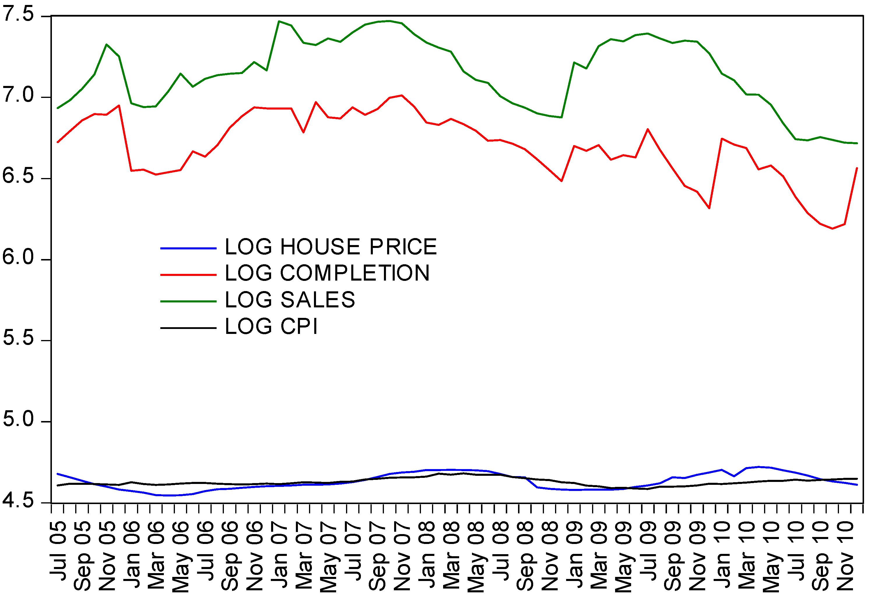
All the data sets were seasonally adjusted using the same X12 procedure [102] and converted into logarithms before the tests. Table 2 statistically describes the data. Figure 4 plots four series.
Table 2. Descriptive statistics for the data (seasonally adjusted using X12).
DefinitionIndex changes in nominal urban new commodity housing for the same period of previous year = 100Completed new commodity housing property (10,000 square meters)Commodity housing property transacted (10,000 square meters)City-specific CPI for the same period of previous year = 100
VariableHOUSE PRICECOMPLETIONSALESCPI
Mean102.89826.071302.02102.42
Median101.72818.241271.60101.76
Maximum112.361110.621756.88107.90
Minimum94.16487.69827.0298.07
Std. Dev.5.16158.27273.372.39
Skewness0.17−0.22−0.060.54
Kurtosis1.802.261.872.67
Jarque–Bera4.302.043.573.46
Probability0.120.360.170.18
Sum6790.7854,520.385,933.136759.9
Sum Sq. Dev.1730.611,628,1504,857,690.0372.53
Figure 4. Log changes in house price, housing completions, sales, and CPI in Shanghai.
Sustainability 07 04524 g004

5. Empirical Results and Discussions

The PP tests rejected the null hypothesis of a unit root in first difference at the 1% level for the four variables: HOUSE PRICE, COMPLETION, SALES, and CPI (Table 3). The ADF tests rejected the null hypothesis of a unit root in first difference at the 1% level for COMPLETION and SALES, 5% level for CPI, and 10% level for HOUSE PRICE. Thus, two conventional unit-root tests consistently suggest that these four variables are I(1).
Table 3. Unit root tests.
ADF
Log of variablekLevelpkFirst differencep
HOUSE PRICE4−3.940.021−3.370.06
COMPLETION1−2.770.211−4.880.00
SALES1−1.870.661−5.170.00
CPI3−2.230.471−3.660.03
PP
HOUSE PRICE5−2.530.324−6.210.00
COMPLETION1−3.000.146−8.020.00
SALES2−1.840.671−7.140.00
CPI5−1.740.724−7.260.00
Notes: Test equations included both the intercept and the trend according to [103]. The lag lengths k were selected using the Schwarz information criterion (SIC) for the ADF tests and the Newey–West (NW) bandwidth technique for the PP tests. The k was set at a minimum and maximum value of 1–12 following [104]. p denotes MacKinnon’s (1996) p-value [105].
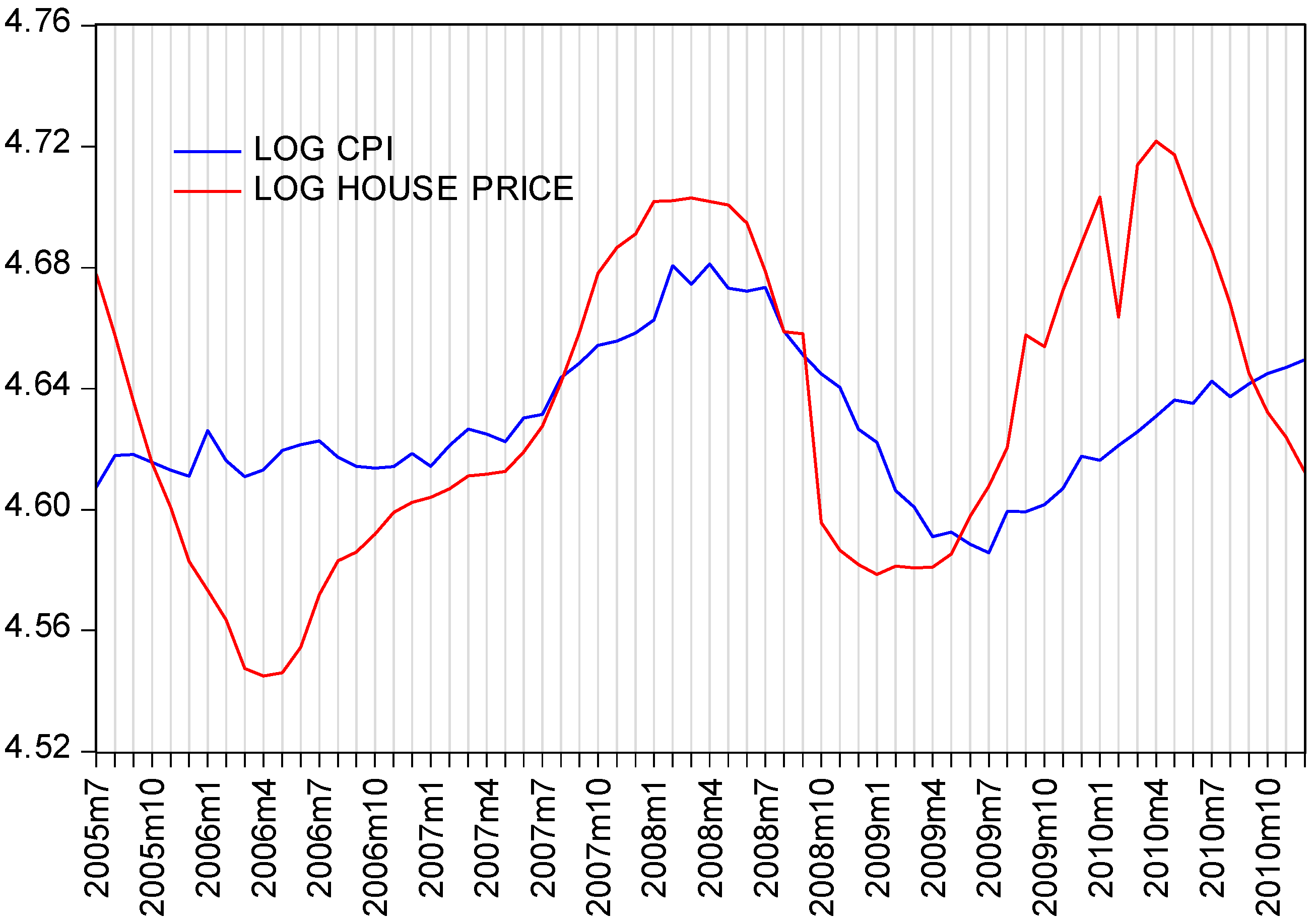
Zivot-Andrews t α * -statistics (Table 4) show that COMPLETION, SALES, and CPI each contains a unit root at the 5% level; however, HOUSE PRICE includes a break date occurring in August 2007. Perron’s t α * -statistics indicate that the null hypothesis of a unit root for the four variables is accepted at the 5% confidence level. Hence, two break date tests consistently show that the three variables COMPLETION, SALES, and CPI are I(1). However, for HOUSE PRICE, two break date tests showed inconsistent results using t α * -statistics. A few other parameters provide further evidence for the unit root property of HOUSE PRICE. In the Perron tests, γ, d, and β are statistically insignificant but μ is highly significant, which indicates that γ, d, and β are equal to zero but μ is not. In the Zivot-Andrews tests, γ and β are statistically insignificant, whereas μ is highly significant, which shows γ and β are equal to zero but μ is not. These parameters generally increased our confidence in the presence of a unit root in HOUSE PRICE. Only θ ≠ 0 suggested a trend stationary process. Moreover, Figure 5 shows that a shift in house prices indeed occurred around August 2007. Nevertheless, the price reached the bottom in January 2009 and peaked once more in April 2010. Therefore, the August 2007 change did not bring about a long-run deterministic (ascending or descending) trend. We treat HOUSE PRICE as an I(1) case.
In the subsequent analyses, we consider that all the four variables are I(1).
Table 4. Zivot–Andrews and Perron structural break tests.
MethodLog of variable αθΓdβμkTb
Zivot–Andrews (Model B)HOUSE PRICE 0.640.020.00-0.001.667Aug 2007
t-statistic8.012.170.07-−0.224.52
COMPLETION −0.72−0.16−0.04-0.0211.3112Apr 2008
t-statistic−1.52−2.41−2.93-2.413.69
SALES 0.240.07−0.01-0.015.3310Aug 2007
t-statistic1.481.28−2.29-1.424.71
CPI 0.490.000.00-0.002.3311Feb 2008
t-statistic3.710.44−3.42-3.243.83
Perron (Model C)HOUSE PRICE 0.530.010.00−0.010.002.208Jun 2007
t-statistic5.410.351.26−0.98−1.434.88
COMPLETION 0.000.77−0.03−0.100.026.536May 2007
t-statistic0.003.98−3.63−0.962.594.67
SALES 0.230.45−0.020.010.015.3110Jan 2008
t-statistic1.373.18−3.220.182.684.50
CPI 0.490.050.000.000.002.3211Dec 2007
t-statistic3.673.23−3.37−0.633.153.75
Notes: The trimming fraction was suggested to be 0.15 [106]. A trimming fraction of 0.23 and 0.24 was arbitrarily used for the Perron test and the Zivot-Andrews test. Therefore, regressions were run from T = 15–51 for the Perron test and from T = 16–50 for the Zivot-Andrews test (T is the sample size). Truncation lag orders k (between 2 and 12) were selected using the data-dependent method [96,104]. t-statistic for the kth term was greater than or equalled to 1.8 in absolute value. Tb was the possible break date. For the Zivot-Andrews test, the critical values for T = 159 were −5.40, −4.84, and −4.57 at the 1%, 5%, and 10% levels, respectively [95]. For the Perron test, the critical values for T = 70 were −6.32, −5.59, and −5.29 at the 1%, 5%, and 10% levels, respectively [96].
Figure 5. Trend changes in house prices and CPI in Shanghai.
Sustainability 07 04524 g005
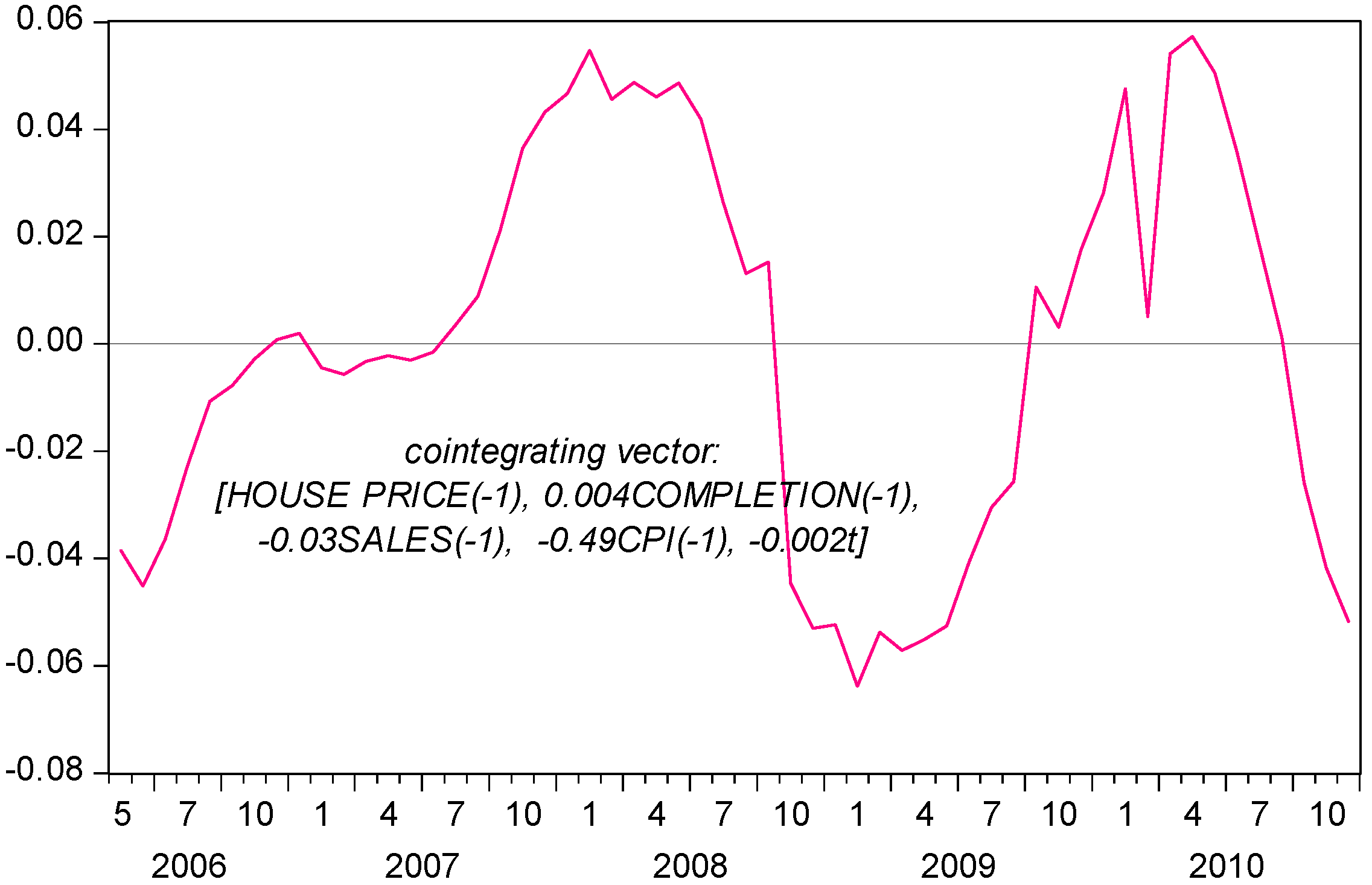
Using the Cheung-Lai finite-sample critical values, the Johansen trace statistics indicate that we could accept the null hypothesis of at most two cointegrating vectors at the 5% confidence level (Table 5). However, Reinsel-Ahn trace corrections show no cointegration at the 5% level. Moreover, when SALES was used as the dependent variable, residual-based tests provided clues to the cointegration (Table 6). Hence, this study suggests a cointegrating vector. Figure 6 shows that the cointegrating vector moves around zero mean.
Table 5. Johansen cointegration trace tests.
rkEigenvalueTrace5%
O-L
5% C&LReinsel–Ahn LRJarque–Bera
(p-value)
LM statistic for no serial correlation
(up to lags, p-value)
090.62147.563.9132.246.9
≤1 0.5493.742.988.829.856.3
(0.43)
14.7
(1, 0.55)
≤2 0.4150.825.953.616.2
≤3 0.3221.512.525.96.85
Notes: r is the null hypothesis of the cointegration rank of at most r. Trace denotes the likelihood ratio trace test statistic. Johansen suggests Models I−V for the trace tests [107]. We chose the model between a lag length of 2–9 [104], which is Model IV [100]. The lag length k was selected by reducing the AIC to the extent possible while maintaining multivariate normality (Jarque-Bera statistic using the square foot of covariance technique [108]) and no serial correlation in the Johansen-type ECM. 5% C&L and 5% O-L denote asymptotical and finite-sample critical values [87,109].
Table 6. Engle-Granger residual-based tests.
Log of dependent variableZα-statisticp-value *
HOUSE PRICE−24.410.11
SALES−49.190.00
COMPLETION−18.690.30
CPI−12.100.67
Notes: The null hypothesis was that the series did not contain a cointegrating vector. Lags were chosen as per the Akaike criterion (AIC). * p-values followed [105].
Figure 6. Cointegrating relationship.
Sustainability 07 04524 g006
Table 7 reports the estimated ECM using HOUSE PRICE as a dependent variable. ECM reports an adjustment coefficient of 0.41, with a significant t-statistic of 1.85, for the error-correction term. Coefficients on COMPLETION are statistically significant in the second, sixth, and ninth lagged terms. Coefficients on SALES are statistically significant in the first, second, sixth, seventh, and eighth lagged terms. Coefficients on CPI are statistically significantly for almost all the nine lagged terms.
Table 7. ECM estimates.
Independent variableLagged termsEstimatest-stat.Independent variableLagged termsEstimatest-stat.
ECt − 1 0.411.85
HOUSE PRICEt − 1−0.97−3.20SALESt − 10.082.27
t − 2−0.87−2.84 t − 20.092.57
t − 3−0.71−2.43 t − 30.031.17
t − 40.050.22 t − 40.020.67
t − 5−0.09−0.42 t − 50.041.54
t − 6−0.19−0.83 t − 60.072.72
t − 70.060.31 t − 70.041.76
t − 8−0.26−1.64 t − 80.051.97
t − 9−0.17−1.23 t − 90.020.86
COMPLETIONt − 10.020.64CPIt − 10.902.00
t − 20.062.38 t − 21.863.80
t − 30.031.14 t − 31.302.65
t − 40.041.56 t − 41.072.34
t − 50.000.04 t − 50.230.52
t − 6−0.08−3.01 t − 6−1.22−2.74
t − 7−0.04−1.39 t − 7−0.41−0.81
t − 8−0.05−1.46 t − 8−1.06−2.13
t − 9−0.08−2.60 t − 9−1.54−3.57
Constant 0.012.47
R-squared 0.87
Adj. R-squared 0.60
F-statistic 3.19
Akaike AIC −6.05
Notes: HOUSE PRICE was the dependent variable. Variables were in logarithms. Data were first differenced.
In ECM, we rejected the null hypothesis that COMPLETION and CPI do not Granger cause HOUSE PRICE at the 1% level (Table 8). We rejected the null hypothesis that SALES does not Granger cause HOUSE PRICE at the 10% level. However, we accepted the null hypothesis that HOUSE PRICE does not Granger cause SALES and CPI at the 10% level.
Furthermore, the weak exogeneity tests rejected the null hypothesis that α11 = 0, α21 = 0, and α31 = 0 at the 7%, 5%, and 2.5% levels, respectively (Table 9). However, the tests accepted the null hypothesis that α41 = 0 at the 10% level. Hence, the variables HOUSE PRICE, SALES, and COMPLETION are not weakly exogenous with respect to the equilibrium relationship. CPI is weakly exogenous relative to the equilibrium relationship. Particularly, Wald2 for the joint hypothesis that the coefficients of all lagged HOUSE PRICE, SALES, and COMPLETION terms are simultaneously equal to zero is 21.7 with a p-value of 0.75 (Table 8). Therefore, CPI does not react to lagged changes in other variables during the long-run system and thus is strongly exogenous with respect to the long-run relationship.
Table 8. Granger causality tests.
Dependentξk = 0Wald-χ2Degree of freedomsp-value
HOUSE PRICECOMPLETION33.990.00
SALES16.990.05
CPI26.990.00
COMPLETIONHOUSE PRICE37.990.00
SALES12.990.16
CPI21.290.01
SALESHOUSE PRICE12.790.18
COMPLETION6.5890.68
CPI6.5590.68
CPIHOUSE PRICE4.7590.94
COMPLETION3.4490.86
SALES9.8190.37
Notes: Variables were in logarithms. Tests were conducted within the estimated ECM.
Table 9. Weak exogeneity tests.
Log of variable in cointegrating vector H 4 * : corresponding adjustment coefficient α = 0 Wald 2Degree of freedomsp-value
HOUSE PRICEα11 = 03.5110.06
COMPLETIONα21 = 04.7210.03
SALESα31 = 05.4010.02
CPIα41 = 01.3610.24
Notes: α was defined in Equation (8). p-values were estimated on the basis of [84].
The equilibrium relationship reflects the demand-supply mechanism suggested in housing economics for the housing market. The coefficient on ECt − 1 is 0.41, suggesting that approximately 41% of any disequilibrium in the last period will be removed at the current time. As indicated by housing economics, changes in housing completions negatively affect changes in house prices in the short run. Short-term price elasticity relative to housing completions is subtle (−0.08). Also, housing completions do not affect house prices in the long run. The “new” housing market in Shanghai may imply that housing completions vary primarily based on short-run factors such as short-term adjustments to savings and credit interest rates, and speculation. Speculative home purchases may have led to excessive forward-looking price expectations by developers. Additionally, as shown in the review section, China does not establish long-run mechanisms in the housing market. It has not levied a tax on housing properties and lacked the land registry system until March 2015. House purchase control policies are changeable. Hence, the developer would speed up construction of new housing properties mainly based on short-run preferential policies and increasing price expectations. The growth in completions would in turn produce an adverse effect on the price.
A long-run positive relationship is suggested between changes in sales and changes in house prices. Sales affect house prices in the short term but not vice versa. The volume elasticity of house prices is 0.03. Hence, we provide further evidence for the search model.
In the short run, changes in CPI positively and significantly affect house prices in nearly all lagged months. Short-term house price elasticities relative to CPI are 0.9 in one month, 1.86 in two months, 1.3 in three months, and 1.07 in four months, respectively. In the long run, CPI positively impacts house prices, but the other three factors do not. The cointegrating vector β indicates that long-term price elasticity relative to CPI is 0.49. Therefore, housing prices have deviated from supply–demand fundamentals and thus are distorted. CPI positively and noticeably influences house prices in the short run and slightly over the long term. Evidence for the effects of CPI on house prices is powerful, at least within the periods considered.

6. Conclusions

A sustainable price may refer to the long-run equilibrium price of time-series variables. The housing policy in China has focused on restraining fast-growing house prices. The government implemented home purchase control over the past three years and had planned to conduct large-scale shanty town redevelopments in the future. In addition, the housing policy reduced concerns regarding investment in and speculative demand for housing properties in 2006−2009. This study reviewed housing market regulation for a few periods since 2006. We contend that inflation might have undermined housing policy that heavily relies on the control of housing demand and supply in the housing sector.
Therefore, we mainly investigated the equilibrium relationships between monthly frequency variables—house price, housing completions, housing sales, and inflation rate—in Shanghai. The data span the period for 2005−2010. Considering finite-sample biases, an equilibrium relationship is suggested using the Johansen trace and Engle-Granger tests.
Housing completions impact house prices in the short run. Tests suggest a positive trading volume-price relationship. Within the relationship, sales influence house prices in the short term. Hence, the empirical evidence supports the housing search model.
A substantial short-run effect of CPI on house prices should have offset that of supply and volume fundamentals. Empirical evidence justifies this argument. Changes in CPI impressively and positively impact house prices in the short run, particularly in four months. Over the long term, CPI positively and slightly impacts house prices; specifically, CPI is a strongly exogenous variable to determine the long-run relationship. The central government has implemented a prudent monetary policy since mid-2013. Hence, the most recent monetary policy is expected to reduce inflation rates significantly and thereby facilitate the realization of sustainable house prices.
However, this study has some limitations. Data unavailability has restricted us from further investigating the individual new or second-hand housing market in Shanghai. We did not collect time-series data on fiscal and credit changes or local demographic migration and land supply, although these macro factors may have significantly influenced house prices.

Acknowledgments

The research herein was supported by a grant from Chengdu University. We extend our heartfelt gratitude to few anonymous referees for their invaluable comments. In addition, we sincerely thank the editor for his/her valuable contribution. The corresponding author is exclusively and entirely responsible for any errors that may exist in this study.

Author Contributions

Dr. Gao Lu Zou and Professor Kwong Wing Chau jointly designed and performed research. Dr. Zou analyzed the data and wrote the paper. All authors read and approved the final manuscript.

Conflicts of Interest

The authors declare no conflicts of interest.

References

  1. NBSC. Yearly Statistical Data. Available online: http://data.stats.gov.cn/ (accessed on 5 October 2012). (In Chinese)
  2. Shanghai Municipal Bureau of Statistics. Shanghai Statistical Yearbook 2011. Available online: http://www.stats-sh.gov.cn (accessed on 8 October 2012). (In Chinese)
  3. Hui, E.C.M.; Yue, S. Housing Price Bubbles in Hong Kong, Beijing and Shanghai: A Comparative Study. J. Real Estate Finance Econ. 2006, 33, 299–327. [Google Scholar] [CrossRef]
  4. Wu, F. Changes in the Structure of Public Housing Provision in Urban China. Urban Stud. 1996, 33, 1601–1628. [Google Scholar] [CrossRef]
  5. Gu, J.F. An Analysis of the Effect of Overseas Funds on the Real Estate Market in Shanghai. World Econ. Stud. 2005, 5, 68–72. (In Chinese) [Google Scholar]
  6. Tu, J.; Zhang, J. What Pushes up the House Price: Evidence from Shanghai. World Econ. 2005, 5, 28–37. (In Chinese) [Google Scholar]
  7. Wang, L. Impact of Urban Rapid Transit on Residential Property Values. Chin. Econ. 2010, 43, 33–52. [Google Scholar] [CrossRef]
  8. Shanghai Municipal Housing Security and Administration Bureau. Notice on the Implementation of the Housing Purchase Policy That the Households in Shanghai or Other Provinces Can Only Once More Purchase a Commodity Housing in Shanghai. Available online: http://www.shfg.gov.cn/ (accessed on 7 June 2013). (In Chinese)
  9. Shanghai Municipal Bureau of Statistics. Shanghai Statistical Yearbook 2013. Available online: http://www.stats-sh.gov.cn (accessed on 8 March 2014).
  10. Rosen, K.T.; Ross, M.C. Increasing Home Ownership in Urban China: Note on the Problem of Affordability. Hous. Stud. 2000, 15, 77–88. [Google Scholar] [CrossRef]
  11. Su, D.Y.; Zhang, Y.X. An Analysis of the Causes of the Supply Shortage of Securitized Homes and Policies. China Real Estate Finan. 2010, 3, 38–40. [Google Scholar]
  12. Liang, S.L.; Du, D.B. Lack of the Justices of Housing Security Policies in China. Urban Issue 2007, 11, 67–70. [Google Scholar]
  13. Ministry of Land and Resources Lists 1457 Idle Plots in China. China News. 5 January 2011. Available online: www.chinanews.com (accessed on 5 January 2011). (In Chinese)
  14. Yu, M. Ministry of Land and Resources announces remediation of the land for real estate development, land idling becomes the biggest problem. People’s Daily. 20 August 2010. Available online: http://paper.people.com.cn/rmrb/html/2010-08/20/nbs.D110000renmrb_01.htm (accessed on 21 August 2010).
  15. State Council. Report on the Work of the Government 2014. Available online: http://www.gov.cn/zhuanti/2014gzbg.htm (accessed on 25 June 2014). (In Chinese)
  16. Kenny, G. Modelling the Demand and Supply Sides of the Housing Market: Evidence from Ireland. Econ. Model. 1999, 16, 389–409. [Google Scholar] [CrossRef]
  17. Ball, M.; Meen, G.; Nygaard, C. Housing Supply Price Elasticities Revisited: Evidence from International, National, Local and Company Data. J. Hous. Econ. 2010, 19, 255–268. [Google Scholar] [CrossRef]
  18. DiPasquale, D.; Wheaton, W.C. Housing Market Dynamics and the Future of House Prices. J. Urban Econ. 1994, 35, 1–27. [Google Scholar] [CrossRef]
  19. Gat, D.; Schwartz, A.L., Jr. Israel’s Housing Market Dynamics: A Tale of Two Sectors. J. Real Estate Lit. 2000, 8, 129–152. [Google Scholar]
  20. Case, K.E.; Shiller, R.J. The Behavior of Home Buyers and Boom and Post-Boom Markets. New Engl. Econ. Rev. 1988. [Google Scholar] [CrossRef]
  21. Hort, K. Prices and Turnover in the Market for Owner-Occupied Homes. Reg. Sci. Urban Econ. 2000, 30, 99–119. [Google Scholar] [CrossRef]
  22. Song, S.; Young, M.; Hargreaves, B. House Price-Volume Dynamics: Evidence from 12 Cities in New Zealand. J. Real Estate Res. 2010, 32, 75–99. [Google Scholar]
  23. Berkovec, J.A.; Goodman, J.L. Turnover as a Measure of Demand for Existing Homes. Real Estate Econ. 1996, 24, 421–440. [Google Scholar] [CrossRef]
  24. Stein, J.C. Prices and Trading Volume in the Housing Market: A Model with Down-Payment Effects. Quart. J. Econ. 1995, 110, 379–406. [Google Scholar] [CrossRef]
  25. Clayton, J.; MacKinnon, G.; Liang, P. Time Variation of Liquidity in the Private Real Estate Market: An Empirical Investigation. J. Real Estate Res. 2008, 30, 125–160. [Google Scholar]
  26. Yiu, C.Y.; Man, K.F.; Wong, S.K. Trading Volume and Price Dispersion in Housing Markets. J. Prop. Res. 2008, 25, 203–219. [Google Scholar] [CrossRef]
  27. Huang, Z.H.; Yu, X.F.; Du, X.J. Empirical Study of the Impact of Land Supply on Housing Price: A Case of Shanghai. Econ. Geogr. 2009, 29, 624–627. (In Chinese) [Google Scholar]
  28. Yu, H. China’s House Price: Affected by Economic Fundamentals or Real Estate Policy? Front. Econ. China 2010, 5, 25–51. [Google Scholar] [CrossRef]
  29. Friedman, M. Studies in the Quantity Theory of Money; University of Chicago Press: Chicago, IL, USA, 1956. [Google Scholar]
  30. Friedman, M. Price Theory; Aldine: Chicago, IL, USA, 1976. [Google Scholar]
  31. Buckley, R.; Ermisch, J. Government Policy and House Prices in the United Kingdom: An Econometric Analysis. Oxford Bull. Econ. Stat. 1982, 44, 273–304. [Google Scholar] [CrossRef]
  32. Fortura, P.; Kushner, J. Canadian Inter-City House Price Differentials. J. Am. Real Estate Urban Econ. Assoc. 1986, 14, 525–536. [Google Scholar] [CrossRef]
  33. Lastrapes, W.D. The Real Price of Housing and Money Supply Shocks: Time Series Evidence and Theoretical Simulations. J. Hous. Econ. 2002, 11, 40–74. [Google Scholar] [CrossRef]
  34. Eichholtz, P.M.A. A Long Run House Price Index:The Herengracht Index, 1628–1973. Real Estate Econ. 1997, 25, 175–192. [Google Scholar] [CrossRef]
  35. Ebrill, L.P.; Possen, U.M. Inflation and the Taxation of Equity in Corporations and Owner-Occupied Housing. J. Money Credit Bank. 1982, 14, 33–47. [Google Scholar] [CrossRef]
  36. Rubens, J.H.; Bond, M.T.; Webb, J.R. The Inflation-Hedging Effectiveness of Real Estate. J. Real Estate Res. 1989, 4, 45–56. [Google Scholar]
  37. Anari, A.; Kolari, J. House Prices and Inflation. Real Estate Econ. 2002, 30, 67–84. [Google Scholar] [CrossRef]
  38. Abelson, P.; Joyeux, R.; Milunovich, G.; Demi, C. Explaining House Prices in Australia: 1970–2003. Econ. Rec. 2005, 81, S96–S103. [Google Scholar] [CrossRef]
  39. People’s Bank of China. China Monetary Policy Report Quarter Four 2013. Available online: http://www.pbc.gov.cn/publish/zhengcehuobisi/591/index.html (accessed on 5 March 2014). (In Chinese)
  40. Koivu, T. Monetary Policy, Asset Prices and Consumption in China. Econ. Syst. 2012, 36, 307–325. [Google Scholar] [CrossRef]
  41. People’s Bank of China; CBRC. Notice on Further Improving Housing Finance Services. Available online: http://www.pbc.gov.cn/ (accessed on 20 October 2014). (In Chinese)
  42. People’s Bank of China. Statistics: Monely Supply. Available online: http://www.pbc.gov.cn/publish/english/963/index.html (accessed on 6 March 2013).
  43. NBSC. Statistical Data: Monthly Statistics. Available online: http://www.stats.gov.cn/ (accessed on 7 March 2013). (In Chinese)
  44. People’s Bank of China. People’s Bank of China Monetary Policy Committee Held a Regular Meeting in the Third Quarter of 2014. Available online: http://www.pbc.gov.cn/publish/diaochatongjisi/133/index.html (accessed on 2 January 2015). (In Chinese)
  45. Currier, K.M. Existence, Uniqueness, and Computation of Sustainable Prices. Math. Soc. Sci. 1994, 27, 105–109. [Google Scholar] [CrossRef]
  46. Spulber, D.F. Scale Economies and Existence of Sustainable Monopoly Prices. J. Econ. Theor. 1984, 34, 149–163. [Google Scholar] [CrossRef]
  47. DiPasquale, D.; Wheaton, W.C. Urban Economics and Real Estate Markets; Prentice-Hall: Upper Saddle River, NJ, USA, 1996. [Google Scholar]
  48. Benson, E.D.; Hansen, J.L.; Schwartz, A.L., Jr.; Smersh, G.T. The Influence of Canadian Investment on U.S. Residential Property Values. J. Real Estate Res. 1997, 13, 231–249. [Google Scholar]
  49. Glaeser, E.L.; Gyourko, J.; Saiz, A. Housing Supply and Housing Bubbles. J. Urban Econ. 2008, 64, 198–217. [Google Scholar] [CrossRef]
  50. Wheaton, W.C. Real Estate “Cycles”: Some Fundamentals. Real Estate Econ. 1999, 27, 209–230. [Google Scholar] [CrossRef]
  51. Kaiser, R.W. The Long Cycle in Real Estate. J. Real Estate Res. 1997, 14, 233–257. [Google Scholar]
  52. Stiglitz, J.E. Symposium on Bubbles. J. Econ. Perspect. 1990, 4, 13–18. [Google Scholar] [CrossRef]
  53. Shiratsuka, S. Asset Price Bubble in Japan in the 1980s: Lessons for Financial and Macroeconomic Stability; Discussion Paper No. 2003-E-15; IMES Institute for Monetary and Economic Studies, Bank of Japan: Tokyo, Japan, 2003. [Google Scholar]
  54. Bourassa, S.C.; Hendershott, P.H.; Murphy, J. Further Evidence on the Existence of Housing Market Bubbles. J. Prop. Res. 2001, 18, 1–19. [Google Scholar] [CrossRef]
  55. Abraham, J.; Hendershott, P. Bubbles in Metropolitan Housing Markets. J. Hous. Res. 1996, 7, 191–207. [Google Scholar]
  56. Hort, K. Determinants of Urban House Price Fluctuations in Sweden 1968–1994. J. Hous. Econ. 1998, 7, 93–120. [Google Scholar] [CrossRef]
  57. Engle, R.F.; Granger, C.W.J. Cointegration and Error Correction: Representation, Estimation and Testing. Econometrica 1987, 55, 251–276. [Google Scholar] [CrossRef]
  58. Granger, C.W.J. Long Memory Relationships and the Aggregation of Dynamic Models. J. Econom. 1980, 14, 227–238. [Google Scholar] [CrossRef]
  59. Granger, C.W.J. Developments in the Study of Cointegrated Economic Variables. Oxford Bull. Econ. Stat. 1986, 48, 213–228. [Google Scholar] [CrossRef]
  60. Engle, R.F.; Hendry, D.F.; Richard, J.F. Exogeneity. Econometrica 1983, 51, 277–304. [Google Scholar] [CrossRef]
  61. Ye, J.P.; Wu, Z.-H. Urban Housing Policy in China in the Macro-Regulation Period 2004–2007. Urban Pol. Res. 2008, 26, 283–295. [Google Scholar] [CrossRef]
  62. State Council. Notice of the General Office of the State Council on Effectively Stablizing Housing Prices. Available online: http://www.gov.cn/ztzl/2006-06/30/content_323694.htm (accessed on 6 March 2013). (In Chinese)
  63. State Council. Opinions of the Ministry of Construction and Other Ministries on Adjusting the Supply Structure of Housing and Stabilizing House Prices, Forwarded by the General Office of the State Council. Available online: http://www.gov.cn/zwgk/2006-05/29/content_294450.htm (accessed on 7 March 2013). (In Chinese)
  64. State Council. Opinions on Faciliating the Healthy Development of the Real Estate Market. Available online: http://www.gov.cn/zwgk/2008-12/21/content_1184227.htm (accessed on 10 March 2013). (In Chinese)
  65. State Council. Report on the Work of the Government 2009. Available online: http://www.gov.cn/test/2009-03/16/content_1260221.htm (accessed on 10 March 2013). (In Chinese)
  66. Guilfoyle, J.P. The Effect of Property Taxes on Home Values. J. Real Estate Lit. 2000, 82, 111–127. [Google Scholar]
  67. Oates, W.E. The Effects of Property Taxes and Local Public Spending on Property Values: An Empirical Study of Tax Capitalization and the Tiebout Hypothesis. J. Polit. Econ. 1969, 77, 957–971. [Google Scholar] [CrossRef]
  68. Dusansky, R.; Ingber, M.; Karatjas, N. The Impact of Property Taxation on Housing Values and Rents. J. Urban Econ. 1981, 10, 240–255. [Google Scholar] [CrossRef]
  69. Central Government. The 11th Five-Year Plan for China’s Economic and Social Development (2006–2010. Available online: http://www.gov.cn/gongbao/content/2006/content_268766.htm (accessed on 7 January 2013). (In Chinese)
  70. State Council. Notice of the State Council on Facilitating the Continuing and Healthy Development of the Real Estate Market. Available online: http://www.gov.cn/zhengce/content/2008-03/28/content_4797.htm (accessed on 8 January 2013). (In Chinese)
  71. State Council. Notice of the Promotion of Stable and Healthy Development of the Real Estate Market (General Office Issue (General Office Issue 2010, No. 4). Available online: http://www.gov.cn/zwgk/2010-01/10/content_1507058.htm (accessed on 7 March 2013). (In Chinese)
  72. State Council. Notice on Further Improving the Work on the Issues About the Real Estate Market Regulation (General Office Issue 2011, No. 1). Available online: http://www.gov.cn/zwgk/2011-01/27/content_1793578.htm (accessed on 8 March 2013). (In Chinese)
  73. Xinhuanet. Focus on the State Council’s Planning of the Adjustment and Promotion of Top Ten Industries. Available online: news.xinhuanet. com (accessed on 3 January 2014).
  74. Wang, B.; Sun, T. How Effective Are Macroprudential Policies in China? IMF Working Paper; International Monetary Fund: Washington, DC, USA, 2013; pp. 22–23. [Google Scholar]
  75. National Bureau of Statistics. China Statistical Yearbook 2011. Available online: www.stats.gov.cn (accessed on 7 January 2013). (In Chinese)
  76. State Council. Notice on Firmly Curbing the Surge in Housing Prices in Some Cities (General Office Issue 2010, No. 10). Available online: http://www.gov.cn/zwgk/2010-04/17/content_1584927.htm (accessed on 15 January 2013). (In Chinese)
  77. Shanghai Municipal Government. Notice of the Opinions of Implementation in Shanghai of the State Council’s Notice of Further Improving the Work of Relevant Issues About Real Estate Market Regulation. Available online: http://www.shfg.gov.cn/ (accessed on 6 July 2013). (In Chinese)
  78. State Council. State Council’s Opinions on Solving the Housing Difficulities in Low-Income Families in Cities. Available online: http://www.gov.cn/zwgk/2007-08/13/content_714481.htm (accessed on 9 July 2013). (In Chinese)
  79. People’s Bank of China. Notice on strengthening management of commercial real estate credit. Available online: http://finance.people.com.cn/GB/1037/6323893.html (accessed on 28 April 2013).
  80. Sina House. Thirty Six out of Fourty Seven Cities That Implement House Purchase Controls Remove the Purchase Control. Available online: http://sh.house.sina.com.cn/news/2014-08-11/09524361293.shtml (accessed on 1 September 2014). (In Chinese)
  81. Xinhuanet. Central Economic Work Conference 2014. Available online: http://news.xinhuanet.com/fortune/2014-12/11/c_1113611795.htm (accessed on 5 January 2015). (In Chinese)
  82. China Securities. Removement of House Purchase Control and Housing Sales Volume and Prices in Chinese Cities. Available online: http://www.cs.com.cn/ssgs/fcgs/201409/t20140910_4508011.html (accessed on 7 January 2015). (In Chinese)
  83. Johansen, S. Statistical Analysis of Cointegration Vectors. J. Econ. Dynam. Contr. 1988, 12, 231–254. [Google Scholar] [CrossRef]
  84. Johansen, S.; Juselius, K. Maximum Likelihood Estimation and Inference on Cointegration—With Applications to the Demand for Money. Oxford Bull. Econ. Stat. 1990, 52, 169–210. [Google Scholar] [CrossRef]
  85. Johansen, S. Estimation and Hypotheses Testing of Co-Integration Vectors in Gaussian Vector Autoregressive Models. Econometrica 1991, 59, 1551–1580. [Google Scholar] [CrossRef]
  86. Engle, R.F.; Yoo, B.S. Forecasting in Co-Integrated Systems. J. Econom. 1987, 35, 143–157. [Google Scholar] [CrossRef]
  87. Cheung, Y.-W.; Lai, K.S. Finite-Sample Sizes of Johansen’s Likelihood Ratio Tests for Cointegration. Oxford Bull. Econ. Stat. 1993, 55, 313–328. [Google Scholar] [CrossRef]
  88. Reinsel, G.C.; Ahn, S.K. Asymptotic Properties of the Likelihood Ratio Test for Cointegration in the Nonstationary Vector Ar Model; Technical Report; Department of Statistics, University of Wisconsin-Madison: Madison, WI, USA, 1988.
  89. Phillips, P.C.B. Optimal Inference in Cointegrated Systems. Econometrica 1991, 59, 283–306. [Google Scholar] [CrossRef]
  90. Dickey, D.A.; Fuller, W.A. Distribution of the Estimators for Autoregressive Time Series with a Unit Root. J. Am. Stat. Assoc. 1979, 74, 427–431. [Google Scholar]
  91. Fuller, W.A. Introduction to Statistical Time Series; John Wiley: New York, NY, USA, 1976. [Google Scholar]
  92. Phillips, P.C.B.; Perron, P. Testing for a Unit Root in Time Series Regression. Biometrika 1988, 75, 335–346. [Google Scholar] [CrossRef]
  93. Nelson, C.R.; Plosser, C.I. Trends and Random Walks in Macroeconomic Time Series. J. Monet. Econ. 1982, 10, 139–162. [Google Scholar] [CrossRef]
  94. Perron, P. The Great Crash, the Oil Price Shock, and the Unit Root Hypothesis. Econometrica 1989, 57, 1361–1401. [Google Scholar] [CrossRef]
  95. Zivot, E.; Andrews, D.W.K. Further Evidence on the Great Crash, the Oil-Price Shock, and the Unit-Root Hypothesis. J. Bus. Econ. Stat. 1992, 10, 251–270. [Google Scholar]
  96. Perron, P. Further Evidence on Breaking Trend Functions in Macroeconomic Variables. J. Econom. 1997, 80, 355–385. [Google Scholar] [CrossRef]
  97. Sen, A. On Unit-Root Tests When the Alternative Is a Trend-Break Stationary Process. J. Bus. Econ. Stat. 2003, 21, 174–184. [Google Scholar] [CrossRef]
  98. Granger, C.W.J. Investigating Causal Relations by Econometric Models and Cross-Spectral Methods. Econometrica 1969, 37, 424–438. [Google Scholar] [CrossRef]
  99. Granger, C.W.J. Some Properties of Time Series Data and Their Use in Econometric Model Specification. J. Econom. 1981, 16, 121–130. [Google Scholar] [CrossRef]
  100. Hendry, D.F.; Juselius, K. Explaining Cointegration Analysis: Part Ii. Energy J. 2001, 22, 75–120. [Google Scholar] [CrossRef]
  101. Johansen, S. Testing Weak Exogeneity and the Order of Cointegration in UK Money Demand Data. J. Pol. Model. 1992, 14, 313–334. [Google Scholar] [CrossRef]
  102. Abeysinghe, T. Deterministic Seasonal Models and Spurious Regressions. J. Econom. 1994, 61, 259–272. [Google Scholar]
  103. Hamilton, H.D. Time Series Analysis, 1st ed.; Princeton University Press: Princeton, NJ, USA, 1994. [Google Scholar]
  104. Ng, S.; Perron, P. Unit Root Tests in Arma Models with Data Dependent Methods for the Selection of the Truncation Lag. J. Am. Stat. Assoc. 1995, 90, 268–281. [Google Scholar] [CrossRef]
  105. MacKinnon, J.G. Numerical Distribution Functions for Unit Root and Cointegration Tests. J. Appl. Econom. 1996, 11, 601–618. [Google Scholar] [CrossRef]
  106. Banerjee, A.; Lumsdaine, R.L.; Stock, J.H. Recursive and Sequential Tests of the Unit Root and Trend Break Hypothesis: Theory and International Evidence. J. Bus. Econ. Stat. 1992, 10, 271–287. [Google Scholar]
  107. Johansen, S. Likelihood-Based Inference in Cointegrated Vector Autoregressive Models, 1st ed.; Oxford University Press: Oxford, UK, 1995. [Google Scholar]
  108. Urzua, C.M. Omnibus Tests for Multivariate Normality Based on a Class of Maximum Entropy Distributions; Advances in Econometrics; JAI Press: Greenwich, CT, USA, 1997; pp. 341–358. [Google Scholar]
  109. Osterwald-Lenum, M. A Note with Quantiles of the Asymptotic Distribution of the Maximum Likelihood Cointegration Rank Test Statistics. Oxford Bull. Econ. Stat. 1992, 54, 461–472. [Google Scholar] [CrossRef]