Article

Sustainable Approaches for Stormwater Quality Improvements with Experimental Geothermal Paving Systems

1
Department of Civil Engineering, Faculty of Engineering and Science, University of Greenwich, Medway Campus, Chatham Maritime, Kent ME4 4TB, UK
2
Water Sustainability Research Centre, Department of Mechanical, Aerospace, and Civil Engineering, Brunel University London, Uxbridge, Middlesex UB8 3PH, UK
*
Author to whom correspondence should be addressed.
Sustainability 2015, 7(2), 1388-1410; https://doi.org/10.3390/su7021388
Submission received: 10 December 2014 / Revised: 8 January 2015 / Accepted: 14 January 2015 / Published: 27 January 2015

Abstract

:
This research assesses the next generation of permeable pavement systems (PPS) incorporating ground source heat pumps (geothermal paving systems). Twelve experimental pilot-scaled pavement systems were assessed for its stormwater treatability in Edinburgh, UK. The relatively high variability of temperatures during the heating and cooling cycle of a ground source heat pump system embedded into the pavement structure did not allow the ecological risk of pathogenic microbial expansion and survival. Carbon dioxide monitoring indicated relatively high microbial activity on a geotextile layer and within the pavement structure. Anaerobic degradation processes were concentrated around the geotextile zone, where carbon dioxide concentrations reached up to 2000 ppm. The overall water treatment potential was high with up to 99% biochemical oxygen demand removal. The pervious pavement systems reduced the ecological risk of stormwater discharges and provided a low risk of pathogen growth.

1. Introduction

Harvesting of stormwater is a promising alternative water resource which can bring multiple benefits to urbanised communities. However, the wide range of stormwater pollutants present in varying concentrations can pose significant public health risks. It is important to reduce pathogen levels in stormwater in addition to other pollutants to ensure safe stormwater harvesting. The general principle of standard permeable pavement systems (PPS) is simply to collect, treat and/or infiltrate freely any surface runoff to support groundwater recharge. Permeable pavement systems are suitable for a wide variety of residential, commercial and industrial applications, yet are confined to light duty and infrequent usage, even though the capabilities of these systems allow for a much wider range of usage. The reason that PPS are traditionally used for light duty surfaces is often because of geotechnical design considerations for structural loading although heavy duty application products are widely available [1,2].
Furthermore, where there is any concern about the possible migration of pollutants into the groundwater, PPS should be constructed with an impermeable layer, and the treated storm water should subsequently be discharged into sustainable drainage systems. Permeable pavement systems could be seen as posing a potential health risk to humans if partially treated runoff contaminated with animal faeces is recycled for domestic use [3]. Animal faeces from dogs, birds and horses droppings are not commonly used pollutants in academic sustainable (urban) drainage system research, because of their potential pathogenic nature. Nevertheless, there are serious health concerns associated with PPS water (particularly if contaminated with faecal matter), which could potentially be recycled within buildings for toilet flushing, watering of lawns and other applications [4].
Bean et al. [5] reported the nutrient removal capabilities of permeable pavements. At two sites in North Carolina, USA, water samples from permeable pavements were compared to runoff from an adjacent asphalt runoff. Total phosphorus, ammonia-nitrogen (NH4-N), and total Kjeldhal nitrogen were significantly lower that the outflow from the asphalt surface [5]. Average removal efficiencies for NH4-N ranged from 86%–88% and Nitrate-Nitrogen (NO3-N) ranged from 48%–65%, respectively [5]. Kadurupokune and Jayasuriya [6] simulated a 17 year period of stormwater quality sampling on a laboratory scaled permeable pavements, using synthetic urban stormwater consisting of mean concentrations of 141 mg/L, 0.24 mg/L, 2.63 mg/L, and 20 mg/L for total suspended solids, total phosphorous, total nitrogen and oil/greases, respectively. The results showed an average removal efficiency of 96%, 95%, 63% and 94% for these parameters [6]. Furthermore, Blecken et al. [7] investigated the effects of varying temperatures for nutrient and sediment removal with biofilters. The study assessed the removal efficiencies of nutrients, total suspended solids, ammonia and total nitrogen, at temperatures ranging from 0 °C–22 °C. The biofilters consisted of varying layers of sand, silt, fine gravel mixed with top soils similar to the sub-base materials used within permeable pavements. The outflow concentrations showed a 90%–95% removal of phosphorous and suspended solids and a relatively high removal of NH4-N especially at higher temperatures which indicated a nitrification effect. The removal rates of nitrogen based compounds occurred via organic nitrogen mineralisation, NH4-N fixation, microbial uptake, nitrification and denitrification under anoxic conditions within the biofilters [7].
Permeable pavements and ground source heat pumps (GSHP) are both commercially available applications, and there is significant knowledge to be gained from these novel combined systems in a research scenario. A combined system has the potential to capture, detain and treat runoff, and to either cool or heat nearby buildings simultaneously. The sub-base is only heated passively during the summer when hot air within an adjacent building needs to be cooled down by transferring access heat to below the permeable pavement. The heat is in fact a waste product that has the additional benefit of enhancing biodegradation within the sub-base. The impact of temperature changes induced by the geothermal heating and cooling system on the water quality could be assessed to determine its impact on runoff treatment and public health indicators. The research aim of this paper is therefore to gauge the stormwater treatment efficiencies for different designs of PPS combined with and without GSHP (Figure 1). The key objectives are to assess the combined PPS and GSHP performance for an indoor and an outside rig, the water quality at the bottom (representing a worst case pollution scenario) of the tanked systems, and the microbial activities under varying temperature patterns. This study focused on the prevention of potentially water-related diseases by treating runoff contaminated with organics and faecal organisms within temperature-controlled PPS. The most non-human contributor of faecal coliforms in urban stormwater are dogs and cats [3,8] and just in one gram of dog faeces, 23 million faecal coliforms can be found [9]. Common symptoms associated with these diseases may include diarrhea, weight loss, nausea and low grade fever [10].
Figure 1. (a) Indoor (b) Outdoor experimental bins for Permeable Pavement Systems with combined PPS-GSHP.
Sustainability 07 01388 g001

2. Construction and Design Methods

2.1. Environmental Conditions and System Components

Two PPS rigs (indoor and outdoor) operated simultaneously in parallel. Each experimental bin was constructed within a 240-litre wheelie bin with a height of 1070 mm; length of 730 mm; a width of 580 mm and maximum loading weight of 96 kg. The indoor PPS was composed of six bins and placed in a temperature-controlled room with a mean ambient temperature of 15.6 °C. The outdoor rig was submerged within the ground and located outdoors where atmospheric temperature conditions prevailed. Nevertheless, the outdoor rig was sheltered from rainfall with a constructed wooden roof, but exposed to air and partial sunlight (Figure 1) as the only source of water onto the PPS rigs came from the simulated rainfall stormwater inflows. The mean outdoor temperatures annually ranged from 3–15 °C throughout the period of analysis from March 2008 to April 2010 with an average temperature of 12.6 °C. All 12 240-litre wheelie-bins were partly filled with inflow water, and operated in batch flow mode, which therefore simulates “real” car park and pavement runoff conditions [2,3]. Influent flows occurred in a batch mode (very short, regular and cyclic inflows) onto the pavement rigs which were mainly assessed for their stormwater treatment capabilities (Figure 2).
Figure 2. Cross section of experimental permeable pavements and ground-source heat pumps not drawn to scale. (Adapted after [3]).
Sustainability 07 01388 g002
Commercially available pre-washed aggregates (granite and limestone) were used for the construction of the sub-base. Their sizes were determined by the manufacturer (Hanson, Formpave, Coleford, England, UK) according to British standards [11,12]. Generally available pavement materials were used; e.g., crushed gravel and rock with defined edges and sizes between 10 and 63 mm. A typical composition of layers comprises a lower sub-base (250 mm), an upper sub-base (100 mm), a geotextile, a clean 5-mm stone layer (50 mm) and finally paving blocks (80 mm) at the top (Figure 1, Figure 2 and Figure 3). The porous Inbitex geotextile made of polyethylene and polypropylene fibres was placed in the top part of the upper base, as this is the area where considerable microbial degradation of pollutants is likely to take place [13]. Either Inbitex on its own or Inbitex together with an impermeable layer (Terram Drainage Composite, Terram Geosynthetics, Gwent, UK), called composite, and were used in the experimental bins. During installation of the experimental systems, reinforced 5-mm polypropylene tubes were placed within the lower sub-base. Their total length (seven to nine loops) was 10 m. Both ends of each tube were located in a plastic water vessel. One of the ends was connected to the pump and the other end was used as an orifice for water discharge. This arrangement provided closed circulation of water (Figure 4). Aquarium heaters (VISI-THERM, Aquarium Systems NEWA, Loughborough, UK) were used to achieve temperature increases. In-line aquarium coolers (Titan 500, Aqua Medic, Bissendorf, Germany) were applied to decrease the temperatures within coils.
Figure 3. Indoor and outdoor combined permeable pavements and ground-source heat pump rigs with design variables. All six (6) bins treated concentrated stormwater containing gully pot liquor with only PPS 1 and PPS 4 treating concentrated stormwater mixed with dog faeces (Adapted after [3]).
Sustainability 07 01388 g003
The heat pump simulation was achieved by the reinforced 5-mm polypropylene tubes placed in the lower sub-base. The starting point of the system began with the pump directing water into the cooler; thereafter circulating through the coils located at the bottom of the bins and returning to the water vessel (Figure 4). This process is repeated for the heating cycle during which the water cooler is switched off and the water heater turned on. This arrangement provided closed circulation of water and achieved higher temperatures (between 20 °C and 30 °C) in a heating cycle and cooler temperatures (<10 °C) in a cooling mode. The Aquarium heaters were used to achieve higher temperatures in the heating cycle (water heater) whilst In-line aquarium coolers were applied to decrease the temperatures within coils for the cooling mode (water cooler) (Figure 4). For both cycles, water circulated through the main water vessel and back to the sub-base zone of the pavement structure, depending on the switching pattern. Digital liquid crystal display (LCD) aquarium thermometers (thermal electrodes) with a measurement range of 50–70 °C were placed at the top and bottom of the tanked pavement system to measure heating and cooling temperatures. As illustrated in Figure 4, temperature measurements were recorded at the water vessel and at the base of pavement rig near the coils submerged under water with the thermal electrodes. Temperature recording times varied throughout the experiment depending on weekly laboratory analyses. The experimental setup followed a safe system design for providing acceptable levels of safety to the researchers as well as other staff and students. The elimination of risk and hazards were carried out by well labelled signs on experiments, indicating the presence of bio-hazards. Weekly safety engineering checks were made by the technicians in identifying any faults with the electrical connections, pumps, heaters, water piping and disposal of stormwater after treatment. A control of substances hazardous to health (COSHH) risk assessment form was filled in everyday by all researchers involved in the experiment.
Figure 4. Schematic of simulated ground-source heating and cooling system showing the integration of permeable pavements with the water heater, water cooler, and polypropylene tubes placed in the lower sub-base saturated water zone (Adapted after [3]).
Sustainability 07 01388 g004

2.2. Operation of the Heating and Cooling Elements

During the cold periods of the first year of research, heat was provided to the sub-base, resulting in a relative increase of the temperature. This arrangement simulated “real” site conditions of the out-flowing water for the indoor rig, and increased relative temperature differences for the outdoor rig. During warm periods, the opposite arrangement was made, and the sub-base subsequently became relatively cold. Reversed water temperature conditions were used to simulate inflow water (warm in summer and cold in winter). The same arrangement was applied for the outdoor rig. The heating and cooling periods for the experimental rigs were controlled by timers, which switched on the heater or coolant to heat up or cool down the geothermal coils submerged beneath the pavement structure. The water pumps ran continuously, the coolers’ minimum temperature was set at 4 °C and thermostats prevented overheating by switching the heaters off when a temperature of 35 °C is achieved. Two main switching patterns existed to mimic the heating and cooling applications of a supermarket in Scotland. The heating and cooling cycles were set as follows:
  • Heating for a 6 month period (colder months in Scotland) October to March. The heating mode was switched on between the hours of 04:00 to 08:00, 09:00 to 11:00, 12:00 to 15:00, 16:00 to 18:00 and 19:00 to 23:00.
  • Cooling for a 6 month period (warmer months in Scotland) April to September. The cooling mode was switched on between 11:00 to 12:00, 13:00 to 14:00, 15:00 to 18:00 and 19:00 to 20:00.
The geothermal heating and cooling cycles were selected based on the account for equipment safety such as overheating and economic constraints such as energy cost escalation if the switching frequency is high.

2.3. Inflow Water Composition and Sample Collection

Stormwater generated by pavements has a limited range of pollution sources. It is highly unlikely to consistently detect animal pathogens from stormwater runoff directed onto the permeable pavements. Hence, the semi-natural concentrated stormwater mixture was used to dose the pavement rigs to maintain consistency in the range of target pollutant concentrations including pathogens.
Water was exchanged twice weekly from March 2008 to April 2010. The influent samples were prepared using a fixed protocol by collecting gully pot liquor (from the same three gully pots across Edinburgh) and fresh dog faeces on the same day of analysis. Even though a standard collection and preparation protocol was used for all samples, large variations in microbial concentrations and the characteristics of the inflow still occurred based on seasonal variations in rainfall events and subsequent wash off into gully pots, and dog faeces strength and quality variations based upon the animals used. The standard protocol used firstly involved mixing a fixed volume of gully pot liquor (0.2 litres) with a fixed volume of de-chlorinated tap water (2 litres) in a plastic beaker. Next, approximately 3.1 grams of dog faeces were subsequently added and mixed properly to obtain a homogenous mixture. By using treated dilution water of sufficient volume, this meant that microbial contamination only came from the gully pot liquors and dog faeces, and also so that the final mixture had sufficient volume so that it could be evenly distributed across the system. The stormwater mixture was prepared to represent typical stormwater pollutant concentrations. However, target pollutant concentrations for the semi-natural stormwater were found to be much higher when compared to typical concentrations found across the UK. The stormwater drained and filtered through to the bottom of each bin and had a retention time of approximately 2 days. Roughly, 2.1–2.5 litres of sample water was slowly collected from the bottom of each bin by a hand lever pump for specific pollutant loading concentration targets and also to ensure enough filtered water enclosed the bins containing geothermal heating-cooling coils. The temperature of the sample was immediately recorded at this stage.

2.4. Carbon Dioxide Monitoring and Sample Collection

The measurement of CO2 characterizes indirectly the microbial activities, which are mirrored by their corresponding carbon dioxide values. A maximum of four horizontal sampling points were chosen for four bins. Four vertical tubes were installed in selected bins from both the indoor rig and outdoor rig, respectively. The first tube was placed at the shallowest point within the pavement structure, the second tube was placed directly below the geotextile layer where the highest microbial activity is expected to occur, the third tube was placed in the upper part of the sub-base and the fourth placed a few centimetres below in the lower sub-base (partly submerged in filtered water). Sampling tubes were open at the bottom and sealed with black silicone rubber on the top. At the top of the silicone, a flexible tube was joined which formed a valve, which was opened during CO2 sampling. The CO2 concentrations were recorded using an automated portable IRGA (Infra Red Gas Analyser) (PP Systems, Hitchin, Hertfordshire, England, UK).

2.5. Water Quality Analysis

American standard methods [14] were used for the analysis of the water quality. A Hanna HI-991300 combined meter was used to measure pH, total dissolved solids, water sample temperatures and conductivity. Dissolved oxygen content and redox potential (ORP) recordings were carried out with a Hanna HI 98201 meter. The five days at 20 °C N-Allylthiourea (nitrification inhibitor) biological oxygen demand (BOD) was determined using the OxiTop IS 12-6 system supplied by WTW (Wissenschaftlich-Technische-Werkstätten GmbH, Weilheim, Germany). Suspended solids were determined using the total filterable residue, dried at 105 °C.
Ortho-phosphate-phosphorous (PO4), ammonia-nitrogen (NH4) and nitrate-nitrogen (NO3) were analysed with traditional chemical methods from the American Public Health Association (APHA) standard methods for the examination of water and wastewater, nutrient analysis manual [14]. Nitrate was reduced to nitrite by hydrazine in alkaline solution and determined at 550 nm by a colorimetric method using an AA3 flow injection analyser (Bran and Luebbe, Norderstedt, Germany), Bran Luebbe AA3 Atoanalyser Methods: G-109-93 and 94 (Bran and Luebbe, Norderstedt, Germany). The detection limits for nutrients tested ranged from 0.01–100 mg/L.
Quantification of microbes was conducted using pour-plate and spread-plate techniques 24 h after sample collection. Dilutions of the samples were prepared in duplicates and 1 mL of sample was poured into a sterile disposable Petri dishes. 15–20 mL of the medium agar was cooled to a temperature of 45 °C into the Petri dishes with sample. The samples were mixed and then incubated along with the blank plates. Soon after incubation the numbers of colonies on the plates were recorded as Colony Forming Units (CFU) per 100 mL. Plate counts were done under microscope in a fume cupboard to prevent pathogenic organisms’ transmission on the researchers.
A nutrient Agar (non-selective growth medium) was used for the growth and analysis of a wide variety of oxygen-tolerant genera such as total heterotrophic bacteria, as one of the key water quality indicators. MacConkey Agar allows for the detection and isolation of Shigella sp. The Slanetz and Bartley Agar were used to favour the growth of Enterococcus sp. where colonies were identified by their red or pink colour. Eosin methylene blue (EMB) agar was used for the detection of Escherichia coli and total coliforms, where E. coli colonies are identified by a blue-black colour with green metallic sheen. All culture media for growing of total heterotrophic bacteria, E. coli, total coliforms, Enterococcus sp. and Shigella sp. were ordered from Oxoid Ltd (Solar House, Mercers Row, Cambridge, UK). Petri plates, filter papers (MF 200 with diameter of 125 mm) and primers were supplied by Fisher Scientific UK (Bishop Meadow Road, Loughborough, UK). Nutrient Agar plates and eosin methylene blue agar plates were incubated at 36 °C ± 1 °C for 2 days. Slanetz and Bartley agar plates were kept at 45 °C for 5 days.

2.6. Techniques Applied for Data Analyses

The analyses of results were performed using Microsoft Excel, Matlab (Version 2007a; Mathworks, Natick, MA, USA) and the self-organising map (SOM) toolbox for application with Matlab designed by the Adaptive Informatics Research Centre (Laboratory of Computer and Information Science, Helsinki University of Technology, Finland). The SOM is a neural network algorithm based on unsupervised learning. System units (neurons) are located on a grid and are represented by a prototype vector. The toolbox focuses on visualisation and data distribution. The net is distributed over the data cloud either by sequential or batch training [15,16]. The use of SOM allows for considerable visual ease of comparison between various systems as well as informs how data is distributed and which parameters have influence on each other. Statistical analysis was performed using IBM SPSS version 18.0. The one-sample Kolmogorov-Smirnov goodness-of-fit test was used to test whether or not a given distribution is significantly different from one hypothesized based on the assumption of a normal distribution [17]. The observed distribution in the one-sample Kolmogorov-Smirnov test of normality is the distribution of the variable in the sample. If the raw stormwater quality data set did not follow a normal distribution, data was transformed using a simple linear transformation method and logarithmic transformation prior to statistical analysis [17]. The analysis of variances (ANOVA) statistical method of testing two or more variables to determine whether their sample means could have been obtained from populations with the same true mean was used [17]. If the water quality effluent variables are similar (from populations with the same mean), the variation within each permeable pavement treatment will be approximately the same as the variations between pavement rigs.

3. Results and Discussion

3.1. Inflow Water Quality

The average concentrations for the inflow water quality parameters throughout the period of analysis are summarised in Table 1.
Table 1. Summary statistics of the water quality of the permeable pavement systems for the inflow (IN) without and with dog faeces as an additional pollutant (P), Sample number, n = 110.
VariableININ + PININ + P
MeanStandard Deviation
Five days at 20 °C Biochemical oxygen demand (mg/L)9.799.811.370.8
Suspended solids (mg/L)132.1258.3151.3190.9
Total dissolved solids (mg/L)57.390.829.134.1
Dissolved oxygen (mg/L)8.98.31.11.5
pH (-)6.86.90.50.6
Conductivity (μS)113.4177.153.957.8
Ammonia-nitrogen (mg/L)0.32.30.41.8
Nitrate-nitrogen (mg/L)1.31.90.84.4
Ortho-phosphate-phosphorus (mg/L)0.83.53.32.2
As a result of the strong variability of the chosen pollutants, the standard deviations for suspended solids were 151.3 mg/L and 190.9 mg/L for the inflow water with and without additional pollutants (dog faeces), respectively. Gully pots on the roadside where sampling occurred linked the surface runoff the continuous inflow of solids into roadside gully pots leads to gradual silting and a high varying suspended and total solids content [13,18]. Similar observations were made for biological oxygen demand (especially with the addition of dog faeces, IN + P) and conductivity. Relatively stable and uniform values were only recorded for pH, dissolved oxygen and nitrate-nitrogen.
Ortho-phosphate-phosphorus mean concentrations were 0.8 mg/L and 3.5 mg/L without and with dog faeces, respectively. The corresponding concentrations for ammonia-nitrogen were 0.3 mg/L and 2.3 mg/L, respectively. It follows that the addition of dog faeces contributed considerably to an increase in nutrients (Table 1 and Table 2). The combination of biodegradation (biological actions) and mainly filtration would have resulted in the removal of phosphorous and nitrogen based compounds.

3.2. Comparison of the Outflow Water Qualities

Table 2 shows the summary statistics of the outflow water quality variables for the indoor and outdoor rigs. The variability of pH was relatively low; maximum standard deviations for both the indoor and outdoor rigs were up to 0.36. Mean values ranged between 7.1 and 7.5. In contrast, the maximum standard deviations for conductivity ranged between 41.8 and 85.9 μS for the indoor and between 32.9 and 90.1 μS for the outdoor rig, respectively. However, the most significant variability was recorded for suspended solids with respect to the outdoor bin 1 and indoor bin 5; standard deviations reached concentrations of 369.5 mg/L and 199.9 mg/L respectively (Table 2).
Mean dissolved oxygen concentrations were similar for both rigs, ranging between 6.4 and 7.6 mg/L, and between 5.8 and 8.3 mg/L for the indoor and outdoor rig respectively (Table 2). Overall reductions in dissolved oxygen for both systems ranged between 1% and 35%. However, the oxygen distribution profile varied considerably within the system. Lowest values were measured near the geotextile and at the bottom, indicating high microbiological activity. The BOD reductions were between 77% and 100%, which indicates a high biodegradation potential [13].
Figure 5, Figure 6 and 
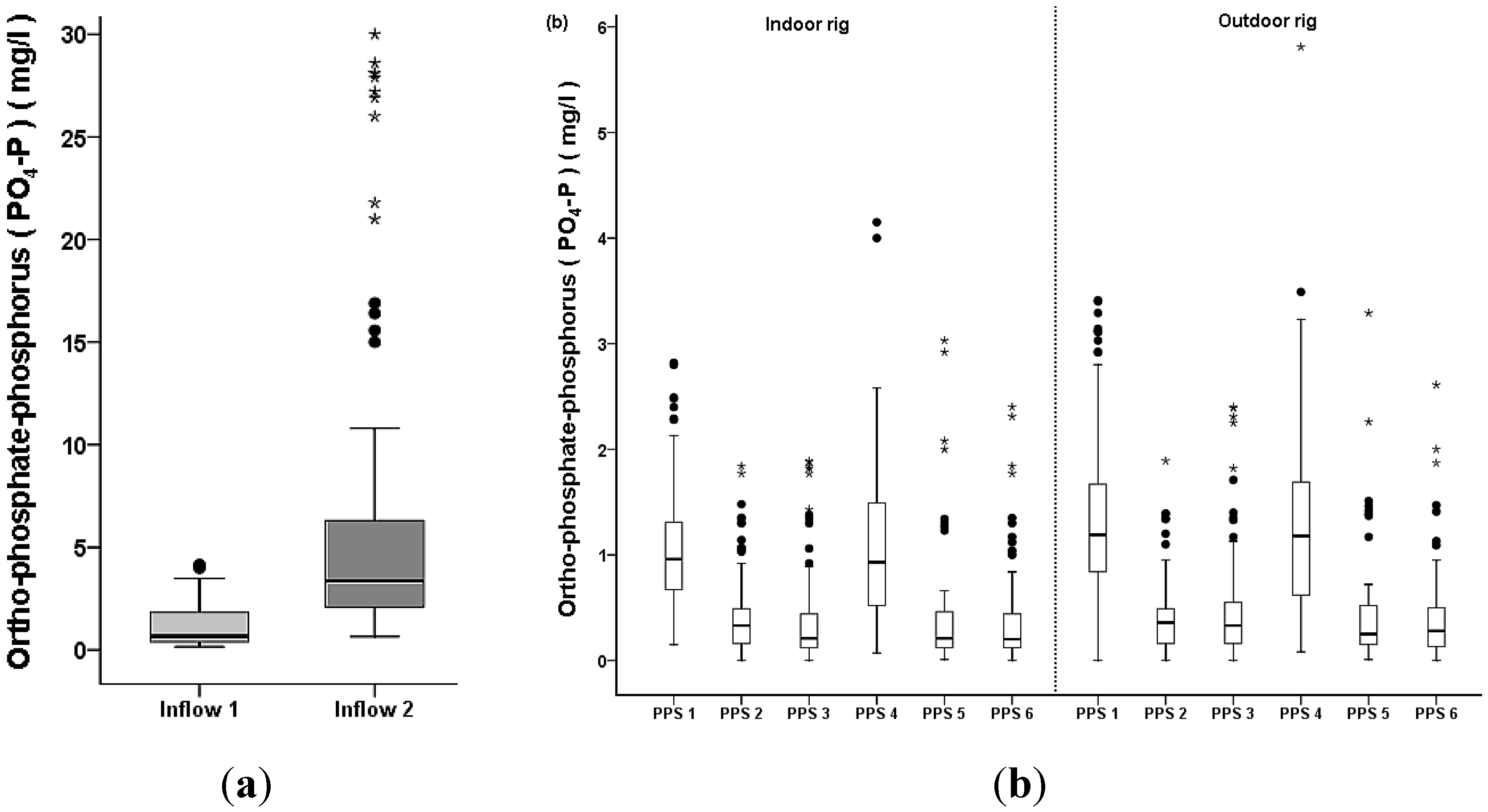
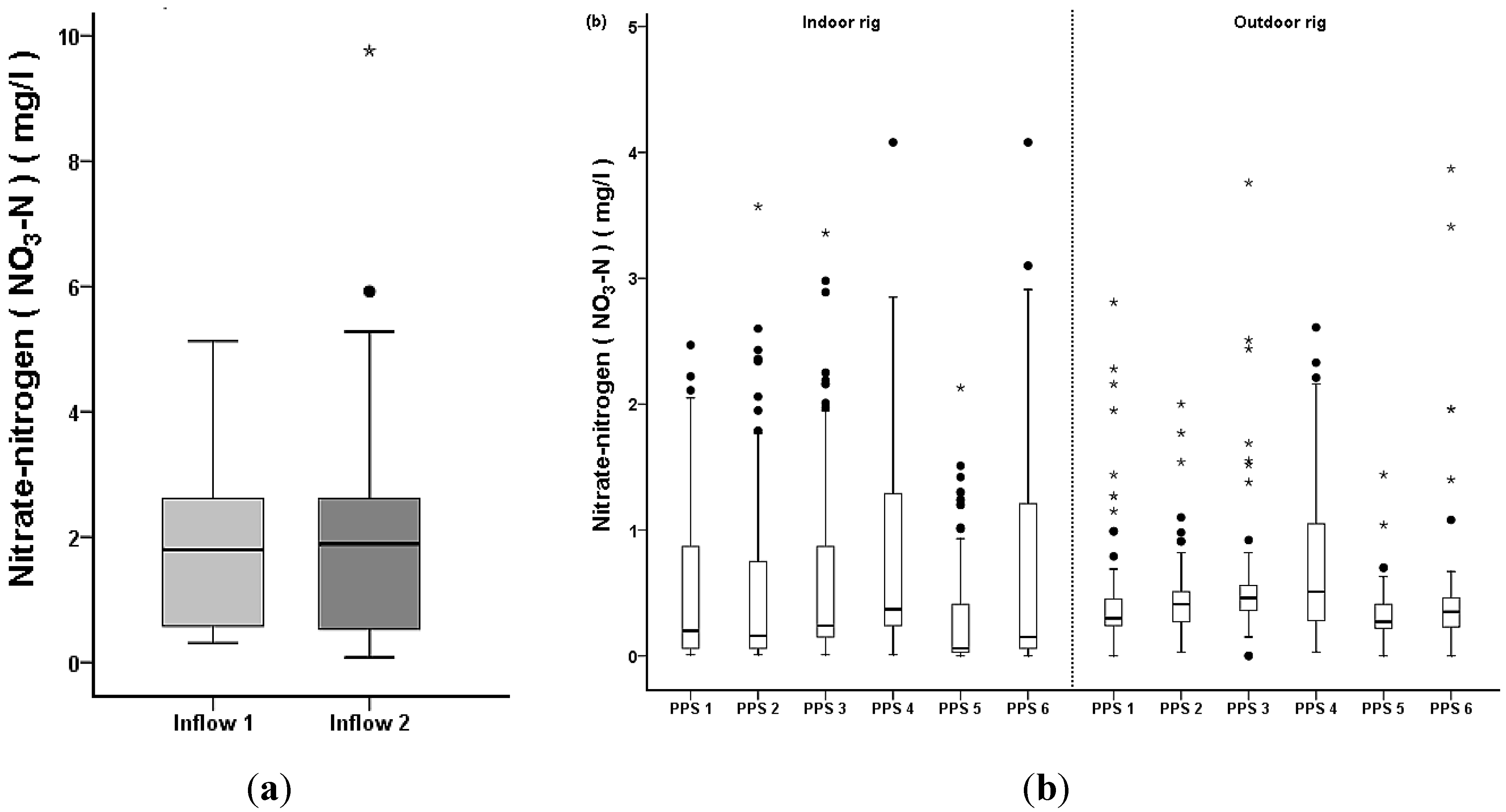
Figure 7 highlight nutrient distributions and show that the ortho-phosphate-phosphorus, ammonia-nitrogen and nitrate-nitrogen concentrations increase considerably with the addition of dog faeces. High reductions of ortho-phosphate-phosphorus (
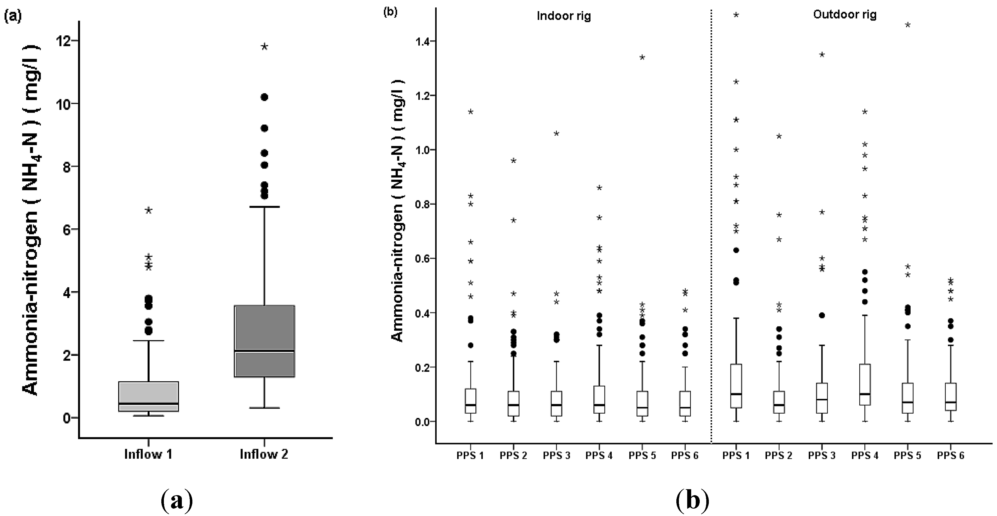
Figure 5) and ammonia-nitrogen (Figure 6) were observed after treatment. For the indoor system, ortho-phosphate-phosphorus mean concentrations were less than 1.4 mg/L (corresponding reduction of 79%). For the outdoor system, concentrations fluctuated between 0.2 and 3.5 mg/L with corresponding reduction rates between 58% and 95%. Ammonia-nitrogen concentrations from urban runoff ranges from 0.1 mg/L–10 mg/L, whilst average concentrations are approximately 25 mg/L from untreated urban domestic wastewater. Hence, the influent concentrations of NH4 matched that of urban stormwater and not domestic wastewater. Ammonia-nitrogen reductions were up to 98% for both systems and the corresponding mean concentrations ranged between 0.07 and 1.09 mg/L for the indoor and between 0.03 and 1.06 mg/L for the outdoor system respectively. The findings indicate relatively high nutrient reductions and/or transformations, which were accelerated during the heating period. However, the mean weekly effluent of nutrients (ammonia-nitrogen, nitrate-nitrogen, nitrite-nitrogen and ortho-phosphate-phosphorous) showed no statistical differences for ANOVA from the heat cycle to the cooling cycle (p > 0.05). Similar results occurred for BOD5 and suspended solids outflow concentrations. Nitrate-nitrogen concentrations varied as a result of organic nitrogen present in the gully pot liquor being converted to NO3-N.
Table 2. Summary statistics of the outflow water quality for the rigs located indoors and outdoors.
VariableStatisticsBin Number
1 *2 **3 **4 *5 **6 **
Indoor Rig (Sample Number, n = 110)
Five-days at 20 °C Biochemical oxygen demand (mg/L)Mean0.81.20.90.60.90.5
SD1.51.70.70.51.00.5
Suspended solids (mg/L)Mean145.1139.4173.3120.3132.7115.5
SD154.1189.9195.3118.3200.0125.4
Total dissolved solids (mg/L)Mean182.7180.4151.8197.6176.3171.6
SD22.833.234.721.127.142.7
Dissolved oxygen (mg/L)Mean6.57.37.67.06.47.2
SD1.82.22.41.81.92.1
pH (-)Mean7.27.57.57.47.47.5
SD0.30.20.20.30.30.3
Conductivity (μS)Mean365.5361.4308.1396.2354.2344.1
SD46.866.870.941.853.986.0
Ammonia-nitrogen (mg/L)Mean0.10.10.10.10.10.1
SD0.20.10.10.10.20.1
Nitrate-nitrogen (mg/L)Mean18.45.94.517.63.24.7
SD16.75.03.218.13.04.1
Ortho-phosphate-phosphorus (mg/L)Mean1.40.40.31.30.30.3
SD0.70.30.40.70.40.4
Outdoor Rig (Sample Number, n = 110)
Five-days at 20 °C Biochemical oxygen demand (mg/L)Mean2.30.80.50.90.60.7
SD3.21.60.71.20.70.9
Suspended solids (mg/L)Mean255.8105.9105.0103.097.470.3
SD369.5115.0131.2101.9124.664.7
Total dissolved solids (mg/L)Mean212.2166.5156.3187.6164.6153.0
SD40.023.716.415.822.116.2
Dissolved oxygen (mg/L)Mean6.28.07.65.88.28.3
SD1.31.61.21.01.51.3
pH (-)Mean7.17.37.37.17.47.4
SD0.20.40.20.30.20.2
Conductivity (μS)Mean428.7333.5314.6383.7329.7307.6
SD90.147.433.067.844.133.3
Ammonia-nitrogen (mg/L)Mean0.10.00.00.00.00.0
SD0.10.00.00.10.00.1
Nitrate-nitrogen (mg/L)Mean8.13.85.55.04.35.1
SD8.63.12.56.03.12.5
Ortho-phosphate-phosphorus (mg/L)Mean1.00.30.21.50.20.2
SD0.90.20.20.80.30.2
SD, standard deviation. * (concentrated stormwater containing dog faeces and gully pot liquor); ** (concentrated stormwater containing gully pot liquor).
Figure 5. Ortho-phosphate-phosphorous concentrations for gully pot liquor and gully pot liquor and dog faeces (a) and outflow concentrations for the indoor and outdoor bins (b). The plots represent the 25th percentile, median and the 75th percentile. The whiskers represent the 10th and 90th percentiles; solid circles represents outliers and stars represents extreme outliers (n = 110).
Sustainability 07 01388 g005
Figure 6. Ammonia-nitrogen concentrations for gully pot liquor and gully pot liquor and dog faeces (a) and outflow concentrations for the indoor and outdoor bins (b). The plots represent the 25th percentile, median and the 75th percentile. The whiskers represent the 10th and 90th percentiles; solid circles represents outliers and stars represents extreme outliers (n = 110).
Sustainability 07 01388 g006
Figure 7. Nitrate-nitrogen concentrations for gully pot liquor and gully pot liquor and dog faeces (a) and outflow concentrations for the indoor and outdoor bins (b). The plots represent the 25th percentile, median and the 75th percentile. The whiskers represent the 10th and 90th percentiles; solid circles represents outliers and stars represents extreme outliers (n = 110).
Sustainability 07 01388 g007
This study continues analysis previously addressed by Scholz and Grabowiecki [13] from 2007–2008 with greater details on the microbial and physiochemical water quality treatability. An increase in nitrate-nitrogen was recorded, as ammonia-nitrogen was broken down [13]. For the indoor and outdoor bins, which received dog faeces, the highest releases of nitrate-nitrogen were recorded. This is likely due to the additional load of nitrogen found by Tota-Maharaj and Scholz [19]. There was also an increase for the indoor bin 6 and the outdoor bin 6 (no faeces, and no heating or cooling). For both outdoor and indoor rigs, nitrate-nitrogen reductions were not observed, as several removal efficiencies were negative due to the low concentrations and reconversion of the nitrite ion to nitrates.
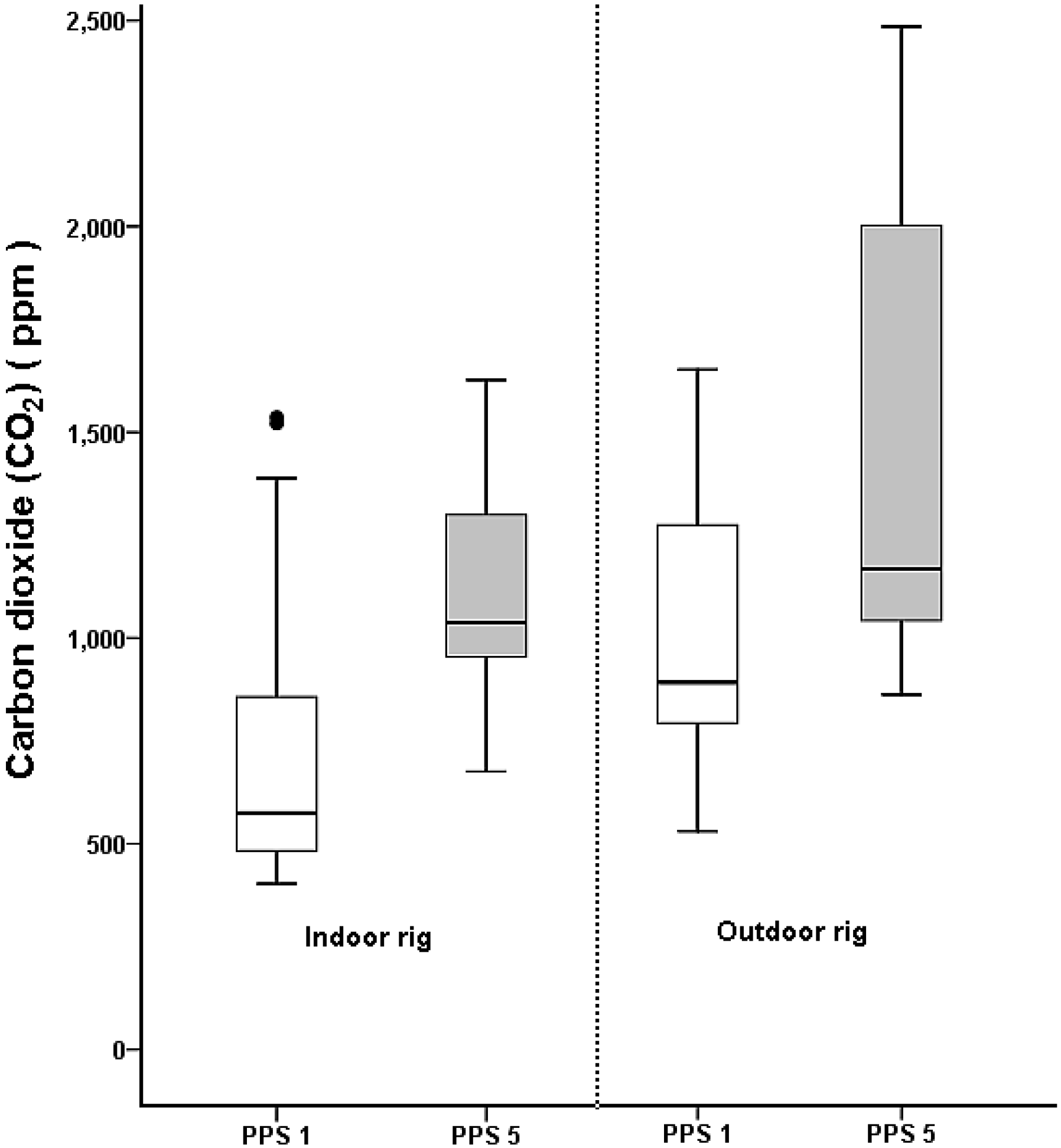
Carbon dioxide levels were similar for the indoor and outdoor rigs, indicating similar activities of microbes (Figure 8). However, only two bins for each system were examined, resulting in 16 sampling points in total. The highest concentrations were recorded close to the first two (i.e., shallowest) sampling points for each bin. This indicated that the most intensive microbial activity took place around the geotextile and the lowest part of the sub-base. Microbiological counts (Table 3) varied considerably for the outdoor system. The spatial distributions of CO2 concentrations generated in the rigs were similar to that reported by Scholz and Grabowiecki [13]. Spatial profiles for PPS with geotextiles from the four horizontal sampling points showed highest concentrations (>2000 ppm) around the geotextile sub-base zone.
Table 3. Mean colony forming unit (CFU/100 mL) counts (rounded to statistically significant numbers) for the rigs effluent of concentrated stormwater between March 2008 and April 2010 (sample number, n = 110).
Rig LocationIndicator BacteriaPPS Number Influent
123456−Dog Faeces+ Dog Faeces
IndoorShigella sp.3.7 × 1021.5 × 1022.5 × 1022.7 × 1024.7 × 1022.1 × 1021.7 × 1044.2 × 105
Enterococus sp.9.0 × 1021.6 × 1021.8 × 1021.9 × 1026.0 × 1011.4 × 1022.1 × 1023.3 × 104
Escherichia coli7.8 × 1031.1 × 1032.8 × 1039.6 × 1037.0 × 1032.9 × 1031.1 × 1051.7 × 106
Total heterotrophs3.7 × 1044.2 × 1047.8 × 1046.6 × 1046.2 × 1049.6 × 1044.4 × 1061.2 × 108
OutdoorShigella sp.3.5 × 1023.1 × 1022.0 × 1023.7 × 1022.2 × 1022.0 × 1023.2× 1039.7 × 104
Enterococus sp.5.0 × 1021.3 × 1025.0 × 1026.0 × 1021.6 × 1022.2 × 1024.1 × 1022.5 × 104
Escherichia coli1.5 × 1055.7 × 1042.9 × 1041.2 × 1055.8× 1035.9× 1036.7× 1042.3 × 106
Total heterotrophs4.9 × 1051.2 × 1053.6 × 1049.6 × 1041.7× 1054.2× 1047.6 × 1063.4 × 101°
Figure 8. Carbon dioxide outflow concentrations for PPS 1 and PPS 5 (indoor and outdoor rig). The plots represent the 25th percentile, median and the 75th percentile. The whiskers represent the 10th and 90th percentiles; solid circles represents outliers (n = 110).
Sustainability 07 01388 g008

3.3. Statistical Analysis

From Table 4, the environmental parameters for all bins (both indoor and outdoor) followed a normal distribution if α > 0.05. On the contrary if α < 0.05, the distribution did not follow normality and was therefore transformed prior to statistical analysis.
Table 4 summarises the distribution of all water quality data (physical, chemical and microbiological) and how this data was distributed over the period of analysis. If the measured parameters followed a normal distribution curve the statistical parameter α > 0.05. It can be seen for water sample temperatures (°C), pH, and dissolved oxygen (mg/L) all followed a normal distribution whilst all other parameters did not. For the cases whereby water quality parameters did not form a normal distribution, the data was transformed prior to the analysis of variance statistical analysis.
One-way ANOVA which has one independent variable was used to test the entire group of Indoor (PPS 1 to PPS6) versus the outdoor group (PPS1 to PPS6) (Table 5) and the effects of carbon dioxide production with PPS 1 versus PPS 5 for both indoor and outdoor, respectively. To test the effects if any, for variations in pavement design for such as (i) treating gully pot liquor and gully pot liquor mixed with dog faeces; (ii) geotextile layer versus geocomposites; and (iii) presence of GSHP, were all analysed with grouped paired ANOVA for a combined indoor and outdoor rigs respectively (Table 6). Grouped pairwise ANOVA comparisons at a significant level of p = 0.05 was applied to test the significant differences between heating and cooling cycles for all water quality parameters effluents within both indoor and outdoor rigs collectively (PPS1, PPS 2, PPS 4 and PPS 5). The statistical tests for pairwise analysis indicate that the water quality variables for each bin (PPS1, PPS2, PPS4, and PPS 5) outflow concentrations differ significantly from each other when p < 0.05 during the heating and cooling cycles (Table 7).
Table 4. One-sample Kolmogorov-Smirnov test for normality. For significance α>0.05 sample follows a normal distribution (in bold).
ParametersIndoor RigOutdoor Rig
PPS 1PPS 2PPS 3PPS 4PPS 5PPS 6PPS 1PPS 2PPS 3PPS 4PPS 5PPS 6
Water sample temperatures (°C)0.8300.1940.9510.8760.1480.8520.8340.9000.7440.6790.6450.827
Geothermal heating/cooling temperatures (°C)0.0000.000¯0.0000.000¯0.0000.000¯0.0000.000¯
pH0.0620.0780.6060.0710.1630.7310.5600.0790.6970.8720.1230.052
Electroconductivity (μS/cm)0.0000.0000.0030.0020.0010.0000.0000.0830.0000.0000.0020.182
Redox potential (mV)0.1130.1040.0990.1540.5710.2460.2920.2550.0830.1630.3420.202
NO3-N (mg/L)0.0000.0000.0000.0000.0000.0000.0000.0020.0000.0000.0010.000
NH4-N (mg/L)0.0000.0000.0000.0000.0000.0000.0000.0000.0000.0000.0000.000
PO4-P mg/L0.0270.0000.0000.0470.0000.0000.0670.0000.0000.0460.0000.001
Total dissolved solids (ppm)0.0420.0410.0680.0060.0140.4240.0430.0480.3300.3510.0790.093
Suspended solids (mg/L)0.0010.0000.0040.0000.0000.0060.0000.0000.0000.0000.0000.000
Turbidity (NTU)0.0020.0000.0010.0000.0000.0030.0010.0000.0000.0000.0000.000
E. coli (CFU/100 mL)0.1760.0140.0010.0020.0280.0000.2300.0190.0100.0200.0000.000
Enterococci sp (CFU/100 mL)0.1380.0080.0000.0000.0000.0000.2400.0180.0020.0010.0150.000
Total coliforms (CFU/100 mL)0.1750.0150.0010.0010.0190.0000.2330.0190.0100.0020.0290.000
Salmonella sp (CFU/100 mL)0.4230.0180.0030.1830.0010.0050.3320.6630.0230.0010.2370.022
Shigella sp (CFU/100 mL)0.4240.0190.0030.1700.0010.0000.2980.6390.0210.0010.2250.024
THB (CFU/100 mL)0.0000.0000.0000.0000.0000.0000.0000.0000.0000.0000.0000.000
BOD (mg/L)0.0000.0000.0000.0000.0000.0000.0000.0000.0010.0000.0010.000
COD (mg/L)0.0020.0000.0030.0030.0010.0000.0510.0000.0170.0000.0010.001
Dissolved oxygen (mg/L)0.1760.2810.0910.0810.0950.1130.9890.7990.1200.2020.4560.530
Carbon dioxide CO2 (ppm)0.000¯¯¯0.000¯0.000¯¯¯0.000¯
ANOVA statistical results for BOD effluent concentrations between the indoor and outdoor rigs showed a strong statistical variation (p < 0.01) (Table 5). BOD effluent concentrations showed variations between (PPS 1 and PPS 4) and (PPS 2 and PPS 5) which compares the differences between the presence of geotextiles (PPS 4) and geocomposites (PPS 1). In addition, variations in concentrations of BOD occurred for (PPS 5 vs. PPS 6) (p < 0.05) and not (PPS 2 vs. PPS 3) (p > 0.05) which shows inconsistencies for BOD outflow concentrations when the pavements systems are integrated with GSHP. ANOVA analysis between PPS 4 and PPS 5 which treated different types of concentrated stormwater (inflows 1 and 2) saw statistical variations in BOD effluent concentrations (p < 0.05) but not (PPS 1 vs. PPS 2). However, during the heating and cooling cycles for PPS 1, PPS 2, PPS 4 and PPS 5, there were no statistical differences for BOD outflow concentrations (p > 0.05).
Table 5. One way ANOVA between in indoor (PPS 1–PPS 6) and outdoor rig (PPS 1–PPS 6), significant values (p < 0.05) in bold.
Water Quality ParametersIndoor Rig & Outdoor Rig
Sum of SquaresSum of SquaresSum of Squares
pH7.45133.980.000
Electroconductivity (μS/cm)4.031 × 1042.750.098
Redox potential (mV)72.500.020.894
Nitrate-nitrogen (NO3-N mg/L)0.521.020.314
Ammonia-nitrogen (NH4-N mg/L)0.639.010.003
Ortho-phosphate-phosphorous (PO4-P mg/L)9.1418.740.000
Total dissolved solids (ppm)1.749 × 10417.350.000
Suspended solids (mg/L)1.561 × 1033.260.072
Escherichia coli (Log10 CFU/100 mL)7.1940.850.000
Enterococci sp. (Log10 CFU/100 mL)5.9832.400.000
Shigella sp. (Log10 CFU/100 mL)5.5356.040.000
Total heterotrophic bacteria (Log10 CFU/100 mL)12.361.070.302
Biochemical oxygen demand (BOD mg/L)349.3926.880.000
Dissolved oxygen (mg/L)0.050.030.85
One-way ANOVA between indoor and outdoor rigs for the effluent NH4-N (mg/L) concentrations showed statistical differences (p < 0.05) (Table 5). Furthermore, NH4-N (mg/L) reductions saw significant variations between (PPS 1 vs. PPS 2) (p < 0.05) with the variable being the type of urban runoff being treated. However, this was not the case for (PPS 4 vs. PPS 5) (p > 0.05) which had similar layouts and treated inflows 1 and 2 separately (Table 6). The presence of geotextiles made a significant contribution for the removal of NH4-N (mg/L) with regards to (PPS 1 vs. PPS 4) and (PPS 2 vs. PPS 5) (p < 0.05). The statistical analysis between the heating and cooling cycles (PPS 1, 2, 4 and 5) also showed significant differences for effluent NH4-N (mg/L) concentrations (p < 0.05) (Table 7). One-way ANOVA between the indoor and outdoor rigs showed a strong statistical variation for E. coli outflow concentrations (p < 0.01), which shows the effects of temperature and environmental conditions on the decline of these bacterial cell colonies (Table 5). With respect to the design variations in pavement systems, the presence of a geotextile membrane (PPS 1 vs. PPS 4) and (PPS 2 vs. PPS 5) for both indoor and outdoor rigs showed a significant difference of E. coli effluent concentrations (p < 0.05). The applications of geothermal heating and cooling (presence of GHP) also saw significant outflow concentrations between (PPS 2 vs. PPS 3) and (PPS 5 vs. PPS 6). In addition, the types of inflow 1 and 2 being treated by the same pavement design (PPS 1 vs. PPS 2) and (PPS 4 vs. PPS 5) showed significant variations for effluent E. coli concentrations. This is expected as inflow 2 spiked with dog faeces contains a higher concentration of E. coli bacterial cells than inflow 1 (gully pot liquor).
Table 6. Paired ANOVA (Indoor and Outdoor rigs) between PPS structure variations and type of urban runoff treated, significant values (p < 0.05) in bold. a (Inflow 1 vs. Inflow 2); b (Geotextile membrane vs. Geocomposite); c (GSHP vs. no GSHP).
Water ParametersPPS (Indoor and Outdoor)
a (1 vs. 2)a (4 vs. 5)b (1 vs. 4)b (2 vs. 5)c (2 vs. 3)c (5 vs 6)
pH0.0000.0000.0000.0000.4890.291
Electroconductivity (μS/cm)0.0000.0000.0000.0000.2460.179
Redox potential (mV)0.7190.1960.1540.2340.3510.406
NO3-N (mg/L)0.2310.0000.0000.0300.0000.001
NH4-N (mg/L)0.0170.1120.0420.0260.4280.881
PO4-P (mg/L)0.0000.0000.0460.0000.9370.331
Total dissolved solids (ppm)0.0950.0000.0000.0000.0000.063
Suspended solids (mg/L)0.2450.0860.0480.0000.5790.016
E. coli (Log10 CFU/100 mL)0.0000.0000.0000.0000.0000.000
Enterococci sp (Log10 CFU/100 mL)0.0000.0000.0000.0000.0000.000
Shigella sp (Log10 CFU/100 mL)0.2390.2190.0000.0180.9590.000
THB (Log10 CFU/100 mL)0.0000.0000.0000.0000.5530.633
BOD (mg/L)0.3720.0220.0000.0000.1640.000
Dissolved oxygen (mg/L)0.0000.0000.0000.0000.0000.000
Table 7. Paired ANOVA between heating and cooling cycles for PPS 1, 2, 4 and 5 (Indoor and Outdoor rigs), significant values (p < 0.05) in bold.
(A) Heating Cylces(B) Cooling CyclesMean Difference (A-B)Std. ErrorSig.
pH0.150.020.000
Electroconductivity (μS/cm)3.156.090.605
Redox potential (mV)33.634.310.000
PO4-P (mg/L)0.050.040.184
NH4-N (mg/L)0.040.020.009
NO3-N (mg/L)0.050.080.485
Total dissolved solids (ppm)3.792.140.077
Suspended solids (mg/L)6.461.480.000
Dissolved oxygen (mg/L)0.580.120.000
BOD (mg/L)0.150.230.512
Escherichia coli (Log10 CFU/100 mL)2.121.820.048
Enterococci sp (Log10 CFU/100 mL)1.471.130.026
Shingallae sp (Log10 CFU/100 mL)1.450.830.000
THB (Log10 CFU/100 mL)4.594.690.425
Throughout the heating and cooling cycles, a significant difference occurred (p < 0.05) for E. coli concentrations between (PPS 1, 2, 4 and 5) (Table 7). For CO2 measurements, ANOVA analysis showed a large significant difference (p < 0.01) between PPS 1 and PPS 5 for both indoor and outdoor rigs regarding the CO2 produced, respectively. The occurrence of higher concentrations of CO2 (ppm) evolved for PPS 5 clearly demonstrates increased microbial activity in and around the geotextile level, when compared to the geocomposite layer in PPS 1. The results show that biodegradation does not only occur at the geotextile layer but evolves at a rapid rate when it is present. PPS 5 when compared to PPS 1 produced a higher percentage of approximately 35% CO2 indicating an increase in microbial activities around this zone. These findings are corroborated by Newman et al. [20]; and Coupe et al. [21] who showed that just above and beneath the geotextile layer within the PPS structure the highest volume of CO2 is produced and O2 is reduced which indicates a higher respiration rate for protozoa and aerobes in the biodegradation process of pollutants.

3.4. Influence of Temperature

Temperature fluctuations due to the presence of the heating or cooling coils had a major impact on the treatment performance of the PPS and the associated microbial community compositions within the sub-bases. During the heating period, temperatures in the bins were between 20 and 25 °C. During the cooling period, the temperature was approximately 5 °C. These temperature recordings contrast air temperatures between 11 and 20 °C during summer and between 3 and 13 °C during winter. Elevated temperatures enhanced biodegradation, but the temperature increases were too low to cause significant growth of potentially pathogenic organisms. The settings for all equipment were the same in the indoor and outdoor rigs, and the mean temperature for the temperature-controlled room was 15.6 °C throughout the year. The temperature of the inflow water and the temperature of the outflow water differed between 0.1 °C and 6.5 °C during cooling. These fluctuations were not high enough to increase the risk of potentially pathogenic organism re-growth.

3.5. Prevention of Water-Related Diseases

The complexity and diversity of microbiological parameters and the fluctuations of temperatures within the PPS-GSHP system results in a complex spatial and temporal relationship between the biological and physiochemical variables justifying the applicability of SOM modelling techniques. The clustering of the SOM neurons provides a summary on the results obtained in the analysis. Different visualisations are realised to explore the interrelationships between the water quality and environmental variables. SOMs consist of the input data layer and the output map layer. Tota-Maharaj and Scholz [19] describe the application of SOM analysis for this permeable pavement experimental setup and how it correlates the inflow and outflow stormwater quality parameters identifying relationships as a visual aid between the selected physiochemical and microbiological measurements. Each neuron of the input layer represents an input variable and has a weighted connection to each of the output layer as shown in Figure 8. The connection weights are adaptively changing at each iteration for the unsupervised training algorithm. The algorithm implements a nonlinear projection from the high-dimensional input space onto a low-dimensional network of neurons normally a 2-dimensional grid [15,16]. The SOM toolbox was applied using the data obtained from both pavement systems to identify the relationship between the influent stormwater quality variables and the microorganism removal efficiency. The prediction was implemented by finding the best matching unit (BMU) within the map for each data set. When specifically analysing microbial contamination, all prior research studies using SOM analysis for permeable pavement experiments have focused on measuring generic indicator organisms, namely Fecal Streptococci and Total Coliforms concentrations [2]. However, this study is unique in that it uses SOM analysis to measure more specific and more virulent pathogenic microbial species, namely Enterococcus sp.; and especially E. coli. E. coli has been responsible for several water borne disease outbreaks globally over recent years, both from food and environmental contamination scenarios [22]. Hence, the self-organising maps for the outdoor bin 1 relate the Enterococcus sp. and E. coli CFU counts of the inflow and outflow to other important water quality variables (Figure 8). The SOM outputs indicate that there is a clear relationship between microbes in the inflow and outflow. There is an apparent positive linear relationship between both microbial parameters, and electrical conductivity and total dissolved solids, indicating that these organisms are potentially present in high numbers, if biodegradation rates are relatively high.
Each input variable has a different weighted connection to each and every one of the SOM neurons (Figure 8 and Figure 9). Since the value of this weight models the influence of the input variables to the activity of each SOM neuron, the distribution of each microbial parameter (Enterococcus sp.; and E. coli) is variable on the SOM (Figure 8 and Figure 9) can be inferred from the corresponding vector of weights. Component plane representation can be thought as a sliced version of the SOM corresponding to a particular component.
Figure 9. Self-organising map for key water quality variables of the outdoor bin 1 including (a) Enterococcus sp.; and (b) E. coli.
Sustainability 07 01388 g009aSustainability 07 01388 g009b

4. Conclusions and Outlook

This study tested the nutrient and organic loading removal effectiveness of combined PPS and GSHP under varying temperature conditions. The combined PPS and GSHP water treatment performance for both rigs was relatively unchanging (60%–90% for most physiochemical and microbial parameters). The ortho-phosphate-phosphorus and ammonia-nitrogen removal rates were relatively high (up to 95%) for influent concentrations with and without dog faeces and the corresponding absolute concentrations fulfilled European urban wastewater treatment standards. Although an increase of nitrate-nitrogen has been observed, the mean outflow concentrations were still well within European standards. The elevated carbon dioxide concentrations and corresponding reductions in biochemical oxygen demand are evidence for the increased microbial activity within the sub-base, especially on the geotextile. Considerable production of carbon dioxide (CO2) occurred with PPS containing a geotextile layer (p < 0.05) when compared to PPS without. The microbial activity during the heating cycle was high leading to an improved treatment performance in terms of biodegradation. There were no significant differences for PPS integrated with GHP during the heating and cooling cycles for PO4-P, NO3-N, TDS, BOD and Total heterotrophic bacteria (THB). The presence of the geotextile layer showed significant differences (p < 0.05) in outflow concentrations for most water quality parameters with the exceptions of PO4-P and NH4-N. The effluent concentrations for indoor bins with regards to NH4-N, PO4-P, E. coli, Enterococci sp, Shigella sp and BOD statistically varied to the outdoor bins outflow concentrations (p < 0.05). However, the risk of a potential transfer of pathogens onto humans was low due to the safe system design and relatively low temperatures within the sub-base. Moreover, the contaminated systems were overly polluted to simulate a worst case scenario, which is unlikely to occur in real applications. The SOM model helped to identify relationships between selected microbial groups and standard water quality variables.

Acknowledgments

The authors would like to thank Piotr Grabowiecki from the Environment Agency, Reading, UK for his technical assistance and experimental setup. Appreciation is extended to Stephen Coupe from the Sustainable Drainage Applied Research Group at Coventry University, UK, Christopher French from the School of Biological Sciences, The University of Edinburgh, Scotland UK and Miklas Scholz from the Civil Engineering Research Centre, University of Salford, Manchester, UK for their scientific advice and support. Hanson Formpave Heidelberg Cement Group sponsored this research project.

Author Contributions

The experimental work, data processing, and modelling work in this study were carried out by Kiran Tota-Maharaj with some follow-on assistance from Parneet Paul. The first draft of the original manuscript was prepared by Kiran Tota-Maharaj and later versions were revised and edited by Parneet Paul before publication.

Conflicts of Interest

The authors declare no conflict of interest.

References

  1. Scholz, M. Wetland Systems to Control Urban Runoff; Elsevier: Amsterdam, The Netherland, 2006. [Google Scholar]
  2. Scholz, M.; Grabowiecki, P. Review of permeable pavement systems. Build. Environ. 2007, 42, 3830–3836. [Google Scholar] [CrossRef]
  3. Tota-Maharaj, K. Permeable Pavements for Urban Stormwater. Runoff Enhancement and Reuse; VDM Verlag Müller: Saarbrücken, Germany, 2011. [Google Scholar]
  4. Scholz, M. Practical Sustainable Urban Drainage System Decision Support Tools. Proc. Instit. Civil Eng. Eng. Sustain. 2006, 159, 117–125. [Google Scholar]
  5. Bean, E.Z.; Hunt, W.F.; Bidelspach, D.A. Evaluation of four permeable pavement sites in eastern North Carolina for runoff reduction and water quality impacts. J. Irrig. Drain. Eng. 2007, 133, 583–592. [Google Scholar] [CrossRef]
  6. Kadurupokune, N.; Jayasuriya, N. Pollutant load removal efficiency of pervious pavements: Is clogging an issue? Water Sci. Technol. 2009, 60, 1787–1794. [Google Scholar] [CrossRef] [PubMed]
  7. Blecken, G.; Zinger, Y.; Deletic, A.; Fletcher, T.D.; Hedstrom, A.; Viklander, M. Laboratory study on stormwater biofiltration: Nutrient and sediment removal in cold temperatures. J. Hydrol. 2010, 394, 507–514. [Google Scholar] [CrossRef]
  8. Hunter, P.R. Waterborne Disease: Epidemiology and Ecology; Wiley: New York, NY, USA, 1997. [Google Scholar]
  9. Alderserio, K.; Wait, D.; Sobsey, M. Detection and Characterization of Male-Specific RNA Coliphages in a New York City Reservoir to Distinguish Between Human and Non-human Sources of Contamination. In Proceedings of the Symposium on New York City Water Supply Studies, Herndon, VA, USA, 14–17 July 1996.
  10. Van der Wel, B. Dog pollution. The Magazine of the Hydrological Society of South Australi 1995. [Google Scholar]
  11. British Standards Institution. Specification for Aggregates from Natural Sources for Concrete; BS 882; British Standards Institution: London, UK, 1992. [Google Scholar]
  12. Highways Agency. Road Pavements, Unbound Cement and Other Hydraulically Bound Mixtures. Manual of Contract Documents for Highway Works Series 800. Volume 1. Specification for Highway Works; Highways Agency: Bedford, UK, 2005. [Google Scholar]
  13. Scholz, M.; Grabowiecki, P. Combined Permeable Pavement and Ground Source Heating Pump Systems to Treat Urban Runoff. J. Chem. Technol. Biotechnol. 2009, 84, 405–413. [Google Scholar] [CrossRef]
  14. Clesceri, L.S.; Eaton, A.D.; Greenberg, A.E.; Franson, M.A.H. Standard Methods for the Examination of Water and Wastewater, 20th ed.; American Public Health Association, American Water Works Association and Water Environment Federation: Washington, DC, USA, 1998. [Google Scholar]
  15. Vesanto, J.H.J.; Alhoniemi, E.; Parhankangas, J. Self-organizing map in Matlab: the SOM Toolbox. In Proceedings of the Matlab. DSP Conference, Espoo, Finland, 16–17 November 1999; pp. 35–40.
  16. Zhang, L.; Scholz, M.; Mustafa, A.; Harrington, R. Application of the Self-organizing Map as a Prediction Tool for an Integrated Constructed Wetland Agroecosystem Treating Agricultural Runoff. Bioresour. Technol. 2009, 100, 539–565. [Google Scholar]
  17. Mac Berthouex, P.; Brown, L.C. Statistics for Environmental Engineers; Lewis Publishers: Boca Raton, FL, USA, 2002. [Google Scholar]
  18. Tota-Maharaj, K.; Grabowiecki, P.; Scholz, M. Energy and Temperature Performance Analysis of Geothermal (Ground Source) Heat Pumps Integrated with Permeable Pavement Systems for Urban Run-off Reuse. Int. J. Sustain. Eng. 2009, 2, 201–213. [Google Scholar] [CrossRef]
  19. Tota-Maharaj, K.; Scholz, M. Modeling of Permeable Pavements for Treatment of Urban Runoff using Self-Organizing Maps. Environ. Eng. Manag. J. 2013, 12, 2273–2287. [Google Scholar]
  20. Newman, A.P.; Pratt, C.J.; Coupe, S.J.; Cresswell, N. Oil bio-degradation in permeable pavements by microbial communities. Water Sci. Technol. 2002, 45, 51–56. [Google Scholar] [PubMed]
  21. Coupe, S.J.; Smith, H.G.; Newman, A.P.; Puehmeier, T. Biodegradation and microbial diversity within permeable pavements. Eur. J. Protistol. 2003, 39, 495–498. [Google Scholar] [CrossRef]
  22. Strachan, N.J.C.; Doyle, M.P.; Kasuga, F.; Rotariu, O.; Ogden, I.D. Dose response modelling of Escherichia coli O157 incorporating data from foodborne and environmental outbreaks. Int. J. Food Microbiol. 2005, 103, 35–47. [Google Scholar] [CrossRef] [PubMed]

