The Improved Cellular Automata and Its Application in Delineation of Urban Spheres of Influence

Abstract

The issue of spatial diffusion and pattern division of traditional cellular automata (CA) has drawn widespread attention and generated extensive work by scholars. However, there are many deficiencies in traditional configurations of CA neighborhoods, which reduce simulation accuracy. The effect of improved methods of traditional configurations of CA neighborhoods is not obvious, and its interoperability is not strong. Therefore, this paper firstly puts forward the concept of the circular neighborhood of CA constrained by the space metric method based on map algebra, and compares the spatial division pattern and anisotropy of different types of neighborhoods in detail. Then, the CA’s weighted diffusion model is discussed to delineate urban spheres of influence in Henan Province. Finally, Weibo data is used to justify a reasonable delineation of urban spheres of influence and can correctly reflect the state of regional development, further proving that improved cellular automata in algorithms and applications have great significance.

1. Introduction

Cellular automata (CA) is a dynamical model which makes discrete evaluations in time according to some local rules in cellular space which consist of discrete cells possessing a finite number of states [1]. Cellular automata, composed of four elements—cells, neighborhoods, rules and time—is a simple model framework providing a new way to simulate complex systems which are essence of how CA realize dynamic simulation. The center cell is a crucial factor for change of states. The local rules constrain the direction of development of cells. Moreover, the definition of neighborhood, including the size and shape of a neighborhood, plays a pivotal role in the state change of cells, the expression of the validity of the rules and formation of spatial pattern.

The earliest cellular automata were developed by von Neumman in the 1940s [2,3]. The range of neighborhoods in this system is mainly the von Neumman neighborhood and Moore neighborhood surrounding the center cell, or the four neighborhoods that remain after removing the four corner-direction cells from the 3 × 3 adjacent domains [4,5]. This kind of neighborhood is homogeneous; that is, the distribution, size and shape of cellular neighborhoods are the same [6]. Cellular automata have drawn more and more attention from multiple fields with further research [7,8,9,10,11], which contributes to the extension of the definition of neighborhoods [12,13]. The distribution of neighborhoods extended to 5 × 5 or 7 × 7 windows [14]. The size of neighborhoods has a great impact on accuracy of simulation results. Therefore, focus should center on selecting the optimal neighborhood template [15]. However, the extension of the definition of neighborhoods previously, when much improvement was made, was merely based on the extension of the standard neighborhoods’ type, which is a compromise on the issue of the complexity and diversity of the definition of neighborhoods of CA, the solution of which usually lies in expanding the scope of neighborhoods.

In recent years, many scholars have come to realize that it is unreasonable to change and diffuse the cellular states in a different-weight dispreading way for standard cellular automata. Isotropic circular neighborhoods have obvious advantages in many fields, but the accurate measurement of raster space is positively correlated with the maximum deviation from the neighborhoods, which means that raster space is difficult to measure and express accurately. Dynamic transformation and composite neighborhood configuration can improve this for by assuring a metric error of around one pixel [16], but the effect is not obvious, and interoperability is not strong; for example, it is difficult to implement with computers and there is a low operational efficiency [17].

According to research on the indicator types and measurement methods of the scope of city, there are two categories: empirical approach and model method. However, it is difficult to obtain the necessary commuting data for the former. In addition, it fails to cover all aspects of the object. As a result, model method turns into the primary research technique [18,19]. The common model methods include the Gravity model [20,21], the Voronoi model [22,23] and Field model [24,25,26], but research on improvements of the cellular automata model and its application to urban spheres of influence is still rare.

This paper puts forward the concept of circular neighborhoods of CA constrained by space metrics based on map algebra though comprehensive and quantitative analysis of a standard neighborhood’s diffusion with different-weight and its effect on the formation of spatial pattern. This paper also compares division pattern of space and anisotropy of different types of neighborhood in detail, and demonstrates that the method is effective and scientific by example.

This paper contains four sections. Section 2 discusses the traditional structure of CA neighborhoods and its diffusion features, and derives the uncertainty law of its resulting spatial pattern; Section 3 introduces the basic idea of map algebra, uses distance constraint strategy to implement the CA’s diffusion in this framework, demonstrates the diffusion feature of neighborhoods with different configurations using anisotropic analysis, and then compares different space patterns with different configurations by simulation data; Section 4 further raises CA’s weighted diffusion model to make delineation of urban spheres of influence in Henan Province. The Weibo data would be used to justify a reasonable delineation of urban spheres of influence and could correctly reflect the state of regional development.

2. Neighborhood Metric of Standard CA

2.1. Understanding and Definition of CA-Diffusion Issues

There is a two-dimensional raster space L (m × m), which gives P fixed points (Generators). Waves begin to diffuse around from each fixed point, and waves from different generators intersect at some time. As a result, they form a pattern with a certain feature. The speed of waves from the same generator is fixed and speed of waves from different generators may vary (diffusion-weighted, will be detailed in the fourth section).Then, the distance from the generator to the wave after moment t is t unit lengths. Therefore, the coincidence points of these waves make-up the dividing line of raster space L, whose distance from the generator is the same, thus the space pattern of L has been formed.

Definition 1. (mathematical definition and rule-making of CA diffusion): there is a two-dimensional raster space L (m × m) and m × m cells. Each cell has three states: $•$ is the generator, $\nabla$ is the developed cell, − is the non-developed cell, and there are P fixed points (generator), P = 1. Suppose $Q$ = {$•$, $\nabla$, −}, $\left|Q\right|$ = 3, and the states of x and its neighborhoods u(x) at the moment t are denoted by x^t and u(x)^t, then the states of the neighborhoods are expressed as:

$$M(u{(x)}^t)=\{h\in Q|\exists y\in u(x),y^t=h\}$$

(1)

The transition of cellular state in different moments is as follows.

$$x^{t+1}=\{\begin{array}{l}•(x^t=-)\cap I{(x)}^t\supseteq \{•\}\\ \nabla (x^t=•)\cap I{(x)}^t\ne \{\varnothing \}\cup (x^t=\nabla )\\ -(x^t=-)\cap I{(x)}^t\supseteq \{-\}\end{array}$$

Transformations: transform constrain

$$•\to \nabla \hspace{1em}I{(x)}^t\ne \{\varnothing \}$$

When the point set of raster space P is 2 or greater, “waves” similar to real waves in nature, which means a continuous, extensional process from the inside out according to the existing template and beginning at the generator (the original point), start to diffuse around each generator and intersect at some time, which forms a pattern with a certain feature, so we can define the spatial process and spatial pattern of CA diffusion as follows:

Definition 2. (mathematical definition and rule-making of spatial pattern formed by CA diffusion): there is a two-dimensional raster of space L (m × m) and m × m Cells. Each cell has four states: $•$ is the generator, $\nabla$ is the developed cell, − is the non-developed cell, and $\ast$ is the boundary cell, meaning the intersection place of waves generated by different generators, which could constitute the boundary line of different generators. There are P fixed points (generator), P is 2 or greater. Suppose $Q$ = {$•$, $\nabla$, −, $\ast$}, $\left|Q\right|$ = 4, and the states of cell x and its neighborhood u(x) at the moment t are denoted by x^t and u(x)^t, then the state of the neighborhoods are expressed as $M(u{(x)}^t)=\{h\in Q|\exists y\in u(x),y^t=h\}$, $I{(x)}^t=M(u{(x)}^t)\cap${$•$, $\nabla$, −, $\ast$}.

The transition of cellular state in different moments is as follows.

$$x^{t+1}=\{\begin{array}{l}•(x^t=-)\cap I{(x)}^t\supseteq \{•\}\\ \nabla (x^t=•)\cap I{(x)}^t\supseteq \{-\}\cup (x^t=\nabla )\\ -(x^t=-)\cap I{(x)}^t\supseteq \{-\}\\ \ast (x^t=•)\cap I{(x)}^t\supseteq \{•\}\cup (x^t=\ast )\end{array}$$

Transformations: transform constrain

$$•\to \nabla \hspace{1em}I{(x)}^t\supseteq \{-\}$$

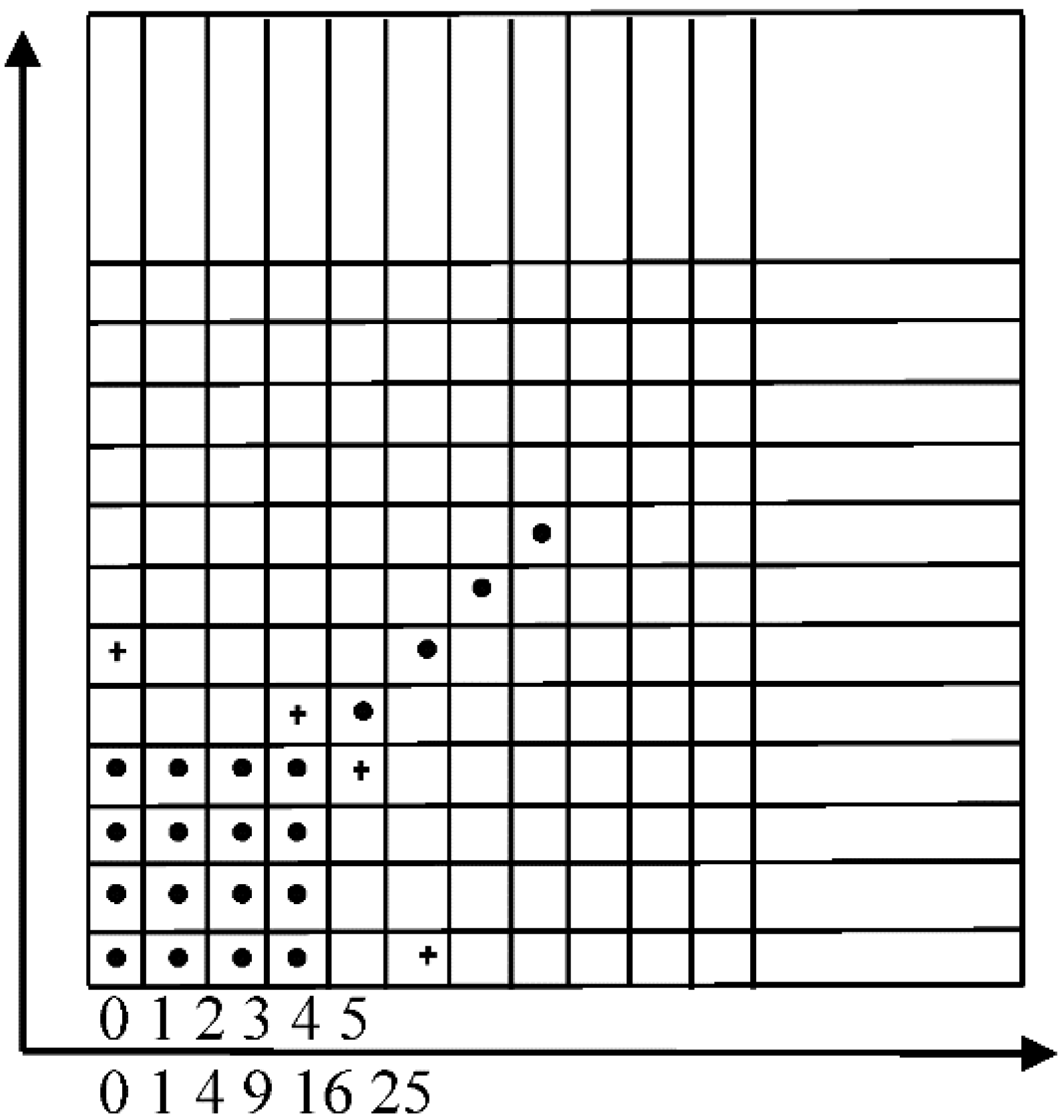
2.2. Standard Metric Methods of Neighborhood and Its Evolution Pattern

Standard metric methods of neighborhood mainly includes: von Neumann, Moore and extended Moore, which can be defined by the following formula:

$$N_{Neumann}=\{v_i=(v_{ix},v_{iy})||v_{ix}-v_{ox}|+|v_{iy}-v_{oy}|\le 1,(v_{ix},v_{iy})\in Z^2\}$$

(2)

In the equation, v_ix, v_iy is coordinate values of neighborhood cells, v_ox, v_oy is coordinate values of the central cells.

Figure 1. Definition of two-dimensional standard cellular automata’s neighborhood. (a) vonNeumann; (b) Moore; (c) Extended Moore.

Figure 1. Definition of two-dimensional standard cellular automata’s neighborhood. (a) vonNeumann; (b) Moore; (c) Extended Moore.

In standard cellular space, the cellular neighborhood adopts a balanced symmetrical configuration with the same overall structure and simple definition. From the perspective of the initial layout, the standard definition of CA’s neighborhoods meets the needs that CA is used to simulate isotropic phenomenon. From the spatial diffusion issues, however, the spatial structure formed by standard definition of CA’s neighborhood has the characteristics of anisotropy, which is just the opposite of the original intention. Figure 2 demonstrates space diffusion’s effect of von Neumann and Moore in different steps (different colors represent different steps): the neighborhood shows obvious anisotropy with the step increases. The von Neumann type grows fast at due east, due south, due north and due west directions, while Moore expands rapidly southeast, southwest, northwest and northeast; the form of the extended Moore type’s diffusion is the same a Moore’s, but the diffusion speed is double.

Figure 2. Step increasing figure of von Neumann and Moore type.

Figure 2. Step increasing figure of von Neumann and Moore type.

Anisotropic expansion model of the standard neighborhood stems from the definition of neighborhood whose direction is of different-weight. To meet the requirement of the expansion of isotropic space, geometrical round is the first choice of the definition of neighborhoods, but this definition is too complicated as well as being difficult to measure accurately in raster space since the inherent properties of raster space, which is usually a square grid, does not allow full circle geometry in order to define the neighborhood’s shape.

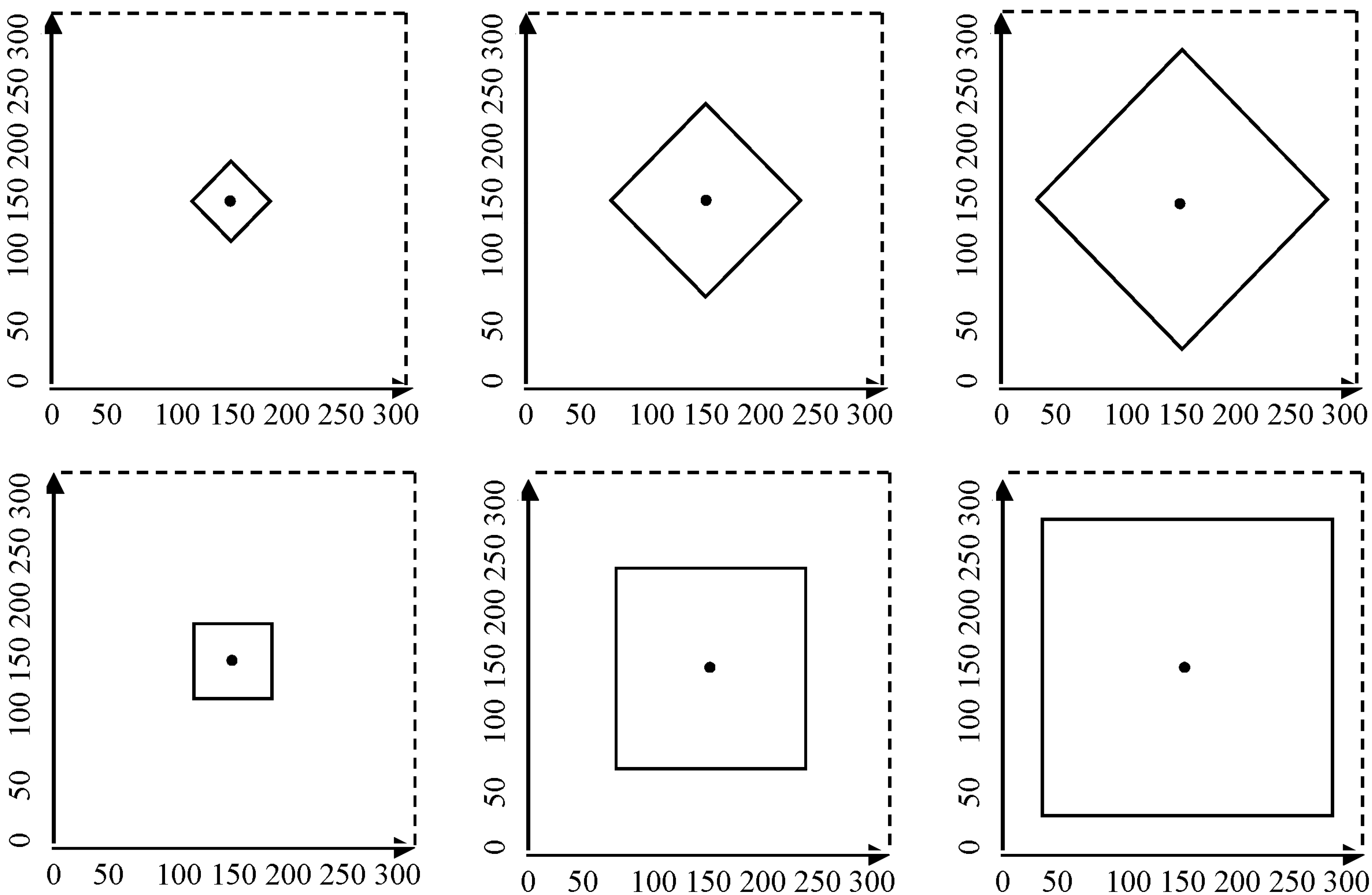
2.3. Uncertainty of Spatial Pattern

Definition of standard neighborhoods appears to be regular and standard. In fact, it is an isotropic and the evolution of spatial pattern of cells tends to be inversed with the increase of the diffusion step, which results in uncertainty of cellular automata simulation and delineation of the spatial pattern. This uncertainty stems from two aspects influenced by the CA model: first, the choice of initial configuration of neighborhoods, the second depends on the relative space position of generators.

The choice of generators for initial configuration of CA’s neighborhoods determines whether there are different rates in different directions. Assume that there are two generators, A and B, whose relative position remains unchanged, and then select the von Neumann-type and Moore-type to divide space, respectively, whose results are shown in Figure 3. As a result of the difference of the generators’ neighborhood configurations, the division results of spatial pattern are different. Movements of the two types’ demarcation line have their own characteristics and the shape of different space regions which belong to their respective generators varies greatly.

Figure 3. Spatial division figure of the von Neumann-type and Moore-type.

Figure 3. Spatial division figure of the von Neumann-type and Moore-type.

In addition, the relative position of the generators impacts the space division results as well. Cellular neighborhoods’ anisotropic becomes more complex when generator’s position changes. Together with the first factor—the initial configuration of neighborhoods—the two factors’ coupling reaction will enhance the uncertainty of the spatial pattern. The Figure 4 shows the spatial division pattern respectively when the angle of the relative positions between the two generators (von Neumann-type and Moore-type) is 0, 30, or 60 degrees.

We can see from Figure 4 that the change of the relative positions impacts the structure of spatial division greatly. Further study found that when the neighborhood configuration of the generators is the same, there is a quantitative relationship between relative position and spatial division as follows:

Definition 3. There are two generators A and B, their neighborhood configuration are von Neumann-type, suppose that the angle by AB and the horizontal line OQ is α (metric of generator’s relative position), the angle by MN (vertical line of AB) and the boundary line CD is β (metric of the degree of boundary line’s deflection), the angle by CD and OQ is γ, then there are relationships as follows:

$$\{\begin{array}{c}\alpha +\beta =\gamma , (\text{A is the center}, \theta \in \left(0,{45}^{\circ }\right){\displaystyle \cup }\left({135}^{\circ },{225}^{\circ }\right){\displaystyle \cup }({315}^{\circ },{360}^{\circ })\\ \alpha -\beta =\gamma , (\text{A is the center}, \theta \in \left({45}^{\circ },{135}^{\circ }\right){\displaystyle \cup }\left({225}^{\circ },{315}^{\circ }\right)\end{array}$$

(3)

In this equation, α β γ, are all acute angles; is the angle of point A relative to point B; the value of γ is 45 degrees because the configuration is fixed.

Definition 4. There are two generators A and B (Figure 5), their neighborhood configurations are Moore-type, suppose that the angle by AB and the horizontal line OQ is α (metric of generator’s relative position), the angle by MN (vertical line of AB) and the boundary line CD is β (metric of the degree of boundary line’s deflection), and the angle by CD and OQ is γ, then their relationships are as follows:

$$\{\begin{array}{c}\alpha =\beta , (\text{A is the center}, \theta \in \left(0,{45}^{\circ }\right){\displaystyle \cup }\left({135}^{\circ },{225}^{\circ }\right){\displaystyle \cup }({315}^{\circ },{360}^{\circ })\\ \alpha +\beta ={90}^{\circ }, (\text{A is the center}, \theta \in \left({45}^{\circ },{135}^{\circ }\right){\displaystyle \cup }\left({225}^{\circ },{315}^{\circ }\right)\end{array}$$

(4)

In this equation, α, β, are all acute angles; γ is a right angle; θ is the angle of point A relative point B.

Figure 4. Comparison of spatial division results of a standard neighborhood under the relative change position.

Figure 4. Comparison of spatial division results of a standard neighborhood under the relative change position.

Figure 5. Diagram of the definition of angle.

Figure 5. Diagram of the definition of angle.

3. Metric of CA’s Neighborhood Based on Map Algebra

The standard neighborhood’s configuration appears to be regular and standard, but actually it is anisotropic. The configuration of neighborhood determines CA’s spatial diffusion pattern and makes space division uncertain, which depends on the choice of relative position and the initial configuration of the generators. Therefore, selecting an isotropic initial neighborhood configuration is very critical for accurate metric and demarcation of space.

In raster space, it is difficult to precisely measure geometric round neighborhood. The approximation to circular using regular polygon is way of compromise, but it is difficult to obtain division accuracy. Dynamic distance transform, based on the six basic configurations, chooses neighborhoods’ configuration in real-time to maintain error within one pixel. However, empirical studies have shown that the error may be more than one pixel. Moreover, the amount of computation of choosing the reasonable configuration is great and the operational efficiency is very low as well.

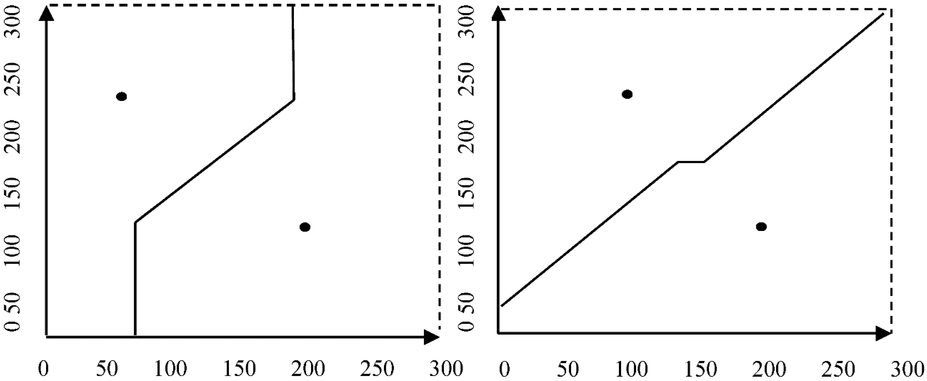
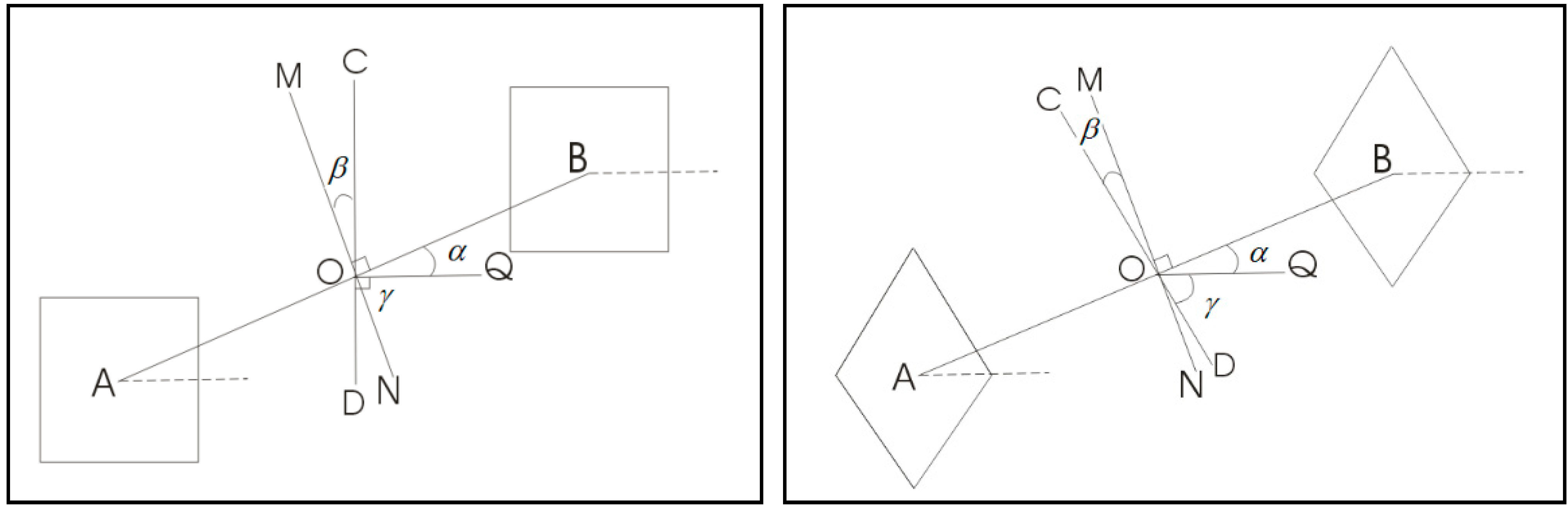
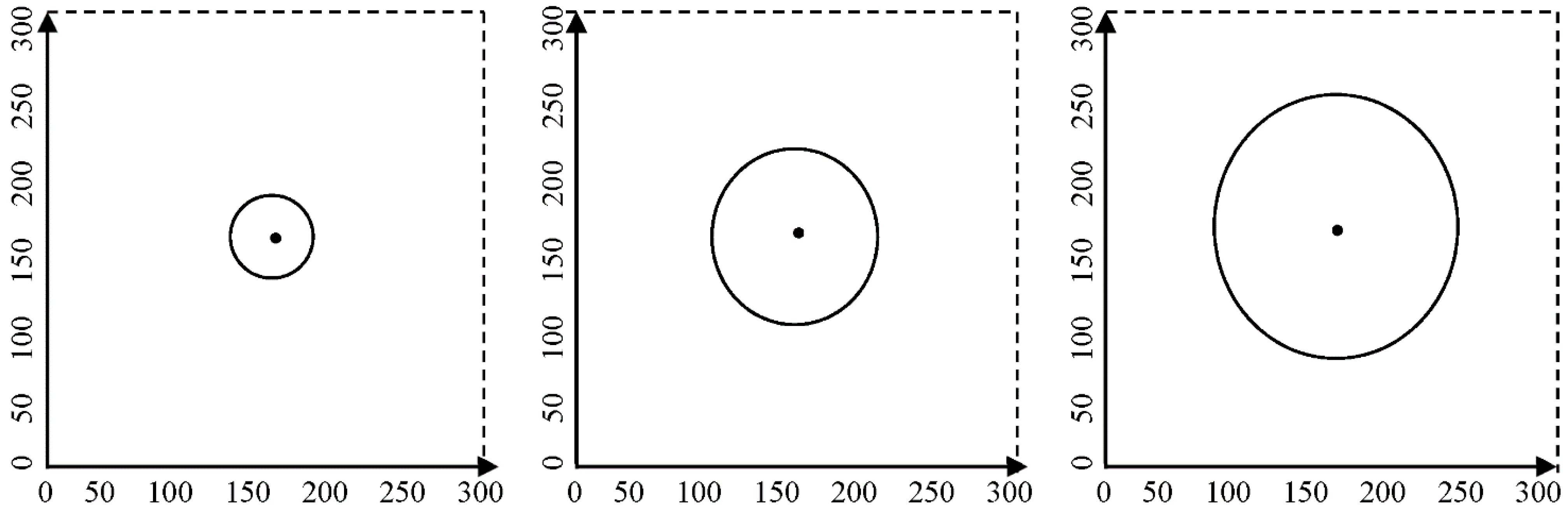
3.1. Basic Principles and the Definition of Diffusion

Map algebra is a relatively mature theory and the algorithm system can conduct spatial analysis and raster computing of map data. It uses transformations and calculations of the spatial raster points set within a certain scale to realize visualization of geographic information and spatial analysis. It is a new type of map theory and its methods based on the basic principles of algebra, which provide a comprehensive representation of the nature of map and map production process from an algebraic point of view. Map algebra can handle the nature of map spatial metrics, preserve geographical significance and ensure the accuracy of geographic data depending on its sophisticated operators.

Metric of CA neighborhoods based on map algebra constitutes the extended mode which uses distance to constrain the center cells under the framework of map algebra, that is, configuration options and identification. Taking von Neumann neighborhood configuration for example, there exist 16 kinds of configurations to be elected under the constraint of distance. The bottleneck of raster space distance metric lies in solving the radical problem of the Euclidean distance; once its root is removed we can carry out integer calculations. As is shown in Figure 6, the crux of the matter can be resolved effectively by adopting raster-square-plane.

The Euclidean distance from a raster (i, j) to the original point on the raster plane is (i² + j²)^1/2, whose coordinate figures in the plane are both integer. Then, its distance and its squared value i² + j² conform to a mapping relationship. Apart from a handful of points (the crosses in Figure 6), such as 3² + 4² = 5² (Pythagorean Theorem), grids located in the triangular plane under the 45° line (the dots in Figure 6) are mostly corresponding with the 1–1 mapping relationship. Obviously, they can be expanded bilateral symmetrically using the line of 45 degrees as the axis of symmetry, respectively. We can also use coordinate axis as the axis of symmetry to extend the plane to the rest three quadrants, called square-planar-raster. As above, we have the raster plane mapped to the square raster plane. For each raster (the center of point), the square value of its Euclidean distance from the origin is recorded as de2.

Figure 6. Raster square planar.

Figure 6. Raster square planar.

$•$: Represent this point is consistent with the one-to-one mapping relationship between its distance and its squared distance value,

$+$: Represent this point isnot consistent with the one-to-one mapping relationship between its distance and its squared distance value.

Definition 5. (mathematical definition and rule-making ofmodified CA diffusion): there is a two-dimensional raster space L (m × m) and m × m cells. Each cell hasthree states: $•$ is the generator, $\nabla$ is the developed cell, −is the non-developed cell. There are P fixed points (generators), P = 1. Suppose $Q$ = {$•$, $\nabla$, −}, $\left|Q\right|$ = 3, the states of cell x and its neighborhood u(x) at the moment t are denoted by x^t, u(x)^t, then the states of the neighborhoods are expressed as $M(u{(x)}^t)=\{h\in Q|\exists y\in u(x),y^t=h\}$, $I{(x)}^t=M(u{(x)}^t)\cap${$•$, $\nabla$, −}.

Take the neighborhood of von Neumann type, for example, and suppose the raster distance of the centralcell in the direction of 45 degrees is D₀:

$$D_0=\{d_t\in D_0|d_t=\frac{\sqrt{2}}{2}t,t\in N\}$$

(5)

Suppose the distance from the other raster to the generator is D₁:

$${\text{D}}_1=\text{de2}(\text{i},\text{j})={(\text{i}-1)}^2+{(\text{j}-1)}^2$$

(6)

Then, take the direction of 45 degrees as the basic distance to inspect the development of the cell center’s neighborhood.

Transition state of cells at different moments has relations as follows:

$$x^{t+1}=\{\begin{array}{l}•(x^t=-)\cap I{(x)}^t\supseteq \{•\}\cap \left|{(D_0-D_1)}^{t+1}\right|>1\\ \nabla (x^t=•)\cap I{(x)}^t\ne \{\varnothing \}\cup (x^t=\nabla )\\ -(x^t=-)\cap I{(x)}^t\supseteq \{-\}\end{array}$$

Transformations: transform constrain

$$\begin{array}{l}•\to \nabla \hspace{1em}I{(x)}^t\ne \{\varnothing \}\\ -\to •\hspace{1em}I{(x)}^t\supseteq \{•\}\cap \left|{(D_0-D_1)}^{t+1}\right|>1\end{array}$$

Definition 6. (mathematical definition and rule-making of spatial pattern formed by modified CA diffusion): there is a two-dimensional raster space L (m × m) and m × m cells. Each cell hasfour states: $•$ is the generator, $\nabla$ is the developed cell, − is the non-developed cell, and * is the boundarycell. There are P fixed points (generators), P is 2 or greater. Suppose $Q$ = {$•$, $\nabla$, −, *}, $\left|Q\right|$ = 4, the states of cell x and its neighborhood u(x) are x^t, u(x)^t, and the state of the neighborhood is equal to $M(u{(x)}^t)=\{h\in Q|\exists y\in u(x),y^t=h\}$, $I{(x)}^t=M(u{(x)}^t)\cap${$•$, $\nabla$, −, *}.

Take the neighborhood of von Neumann type, for example, and suppose the rasterdistance of the central cell in the direction of 45 degrees is D₀:

$$D_0=\{d_t\in D_0|d_t=\frac{\sqrt{2}}{2}t,t\in N\}$$

(7)

Suppose the distance from other raster to the generator is D₁:

$${\text{D}}_1=\text{de2}(\text{i},\text{j})={(\text{i}-1)}^2+{(\text{j}-1)}^2$$

(8)

Then, take the direction of 45 degrees as the basic distance to inspect whether the center cell’s neighborhood is developed or not.

Transition of the cell’s state at different moments has relations as follows:

$$x^{t+1}=\{\begin{array}{l}•(x^t=-)\cap I{(x)}^t\supseteq \{•\}\cap \left|{(D_0-D_1)}^{t+1}\right|>1\\ \nabla (x^t=•)\cap I{(x)}^t\supseteq \{-\}\cup (x^t=\nabla )\\ -(x^t=-)\cap I{(x)}^t\supseteq \{-\}\\ \ast (x^t=•)\cap I{(x)}^t\supseteq \{•\}\cap \left|{(D_0-D_1)}^{t+1}\right|>1\cup (x^t=\ast )\end{array}$$

Transformations: transform constrain

$$\begin{array}{l}•\to \nabla \hspace{1em}I{(x)}^t\supseteq \{-\}\\ -\to •\hspace{1em}I{(x)}^t\supseteq \{•\}\cap \left|{(D_0-D_1)}^{t+1}\right|>1\\ •\to \ast \hspace{1em}I{(x)}^t\supseteq \{•\}\cap \left|{(D_0-D_1)}^{t+1}\right|>1\end{array}$$

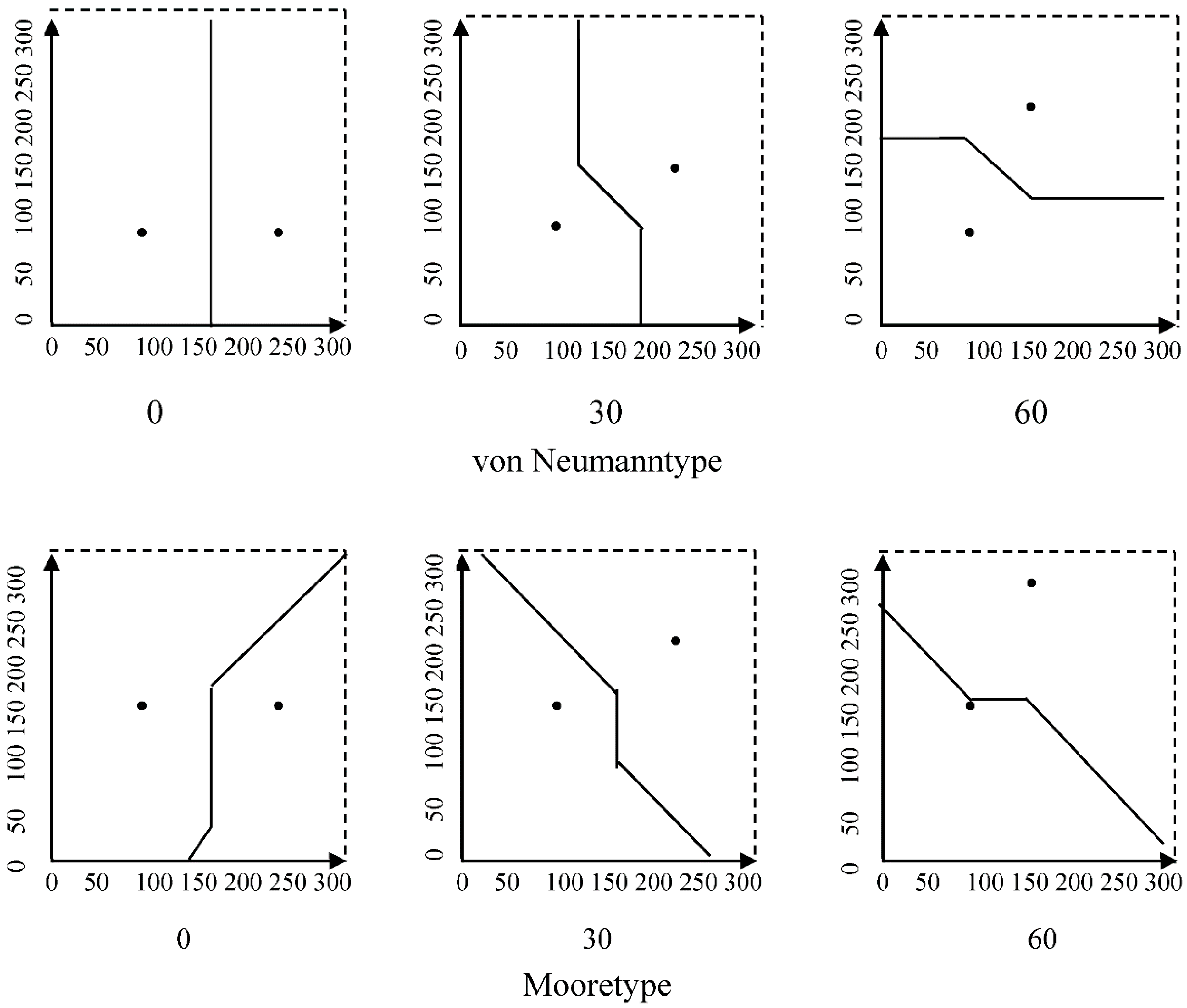
3.2. Improved Metric Method of Neighborhoods and Its Evolution Pattern

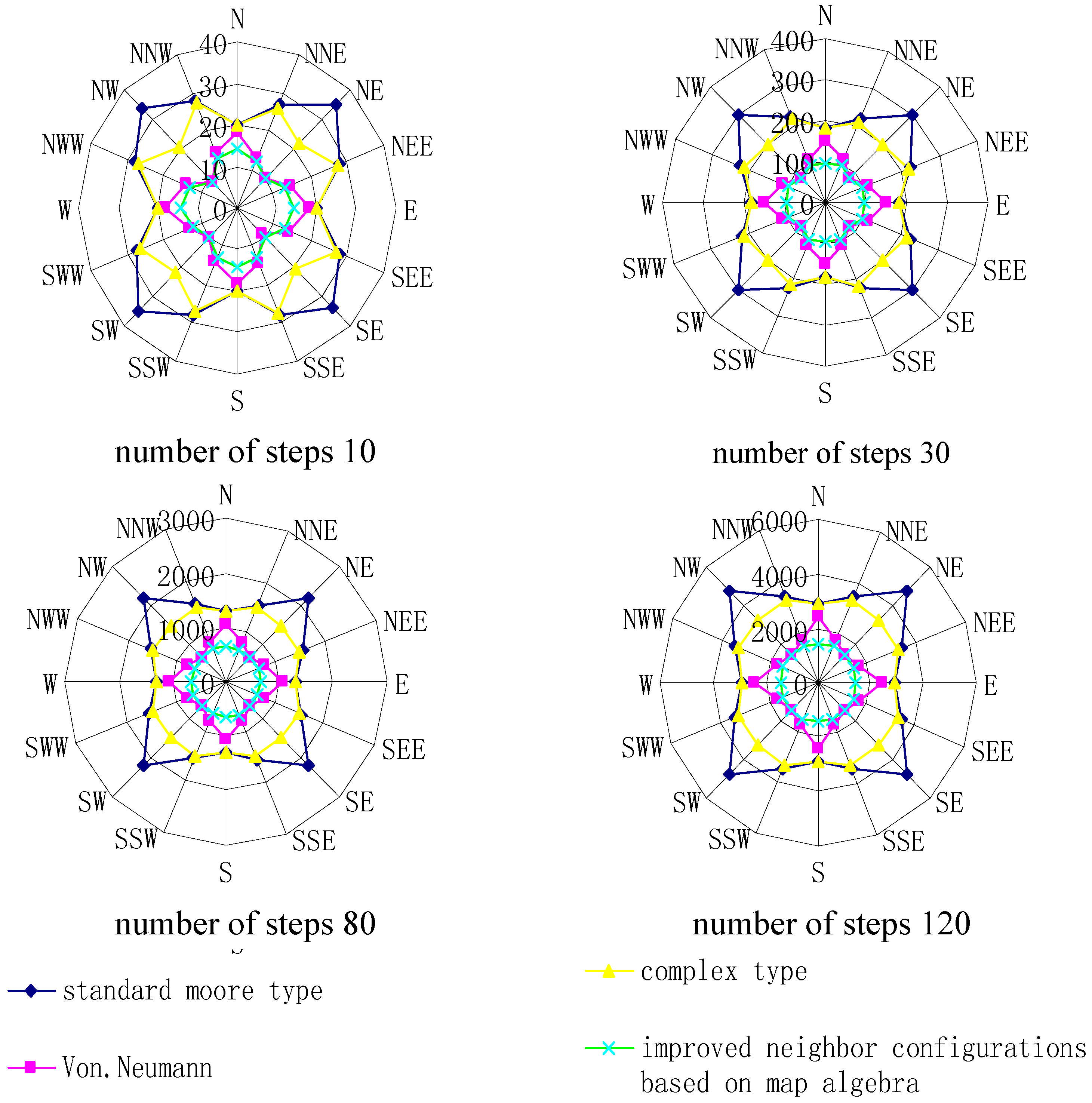
Anisotropy of von Neumann-type neighborhoods is revealed in rapid expansion in the direction of 0, 90, 180, and 270 degrees. According to Map Algebra by Hu [17], there is no error in distance calculation using raster-square-plane and the only error exists in rasterizing entity and rounding after radicand. Moreover, both types of errors are less than 0.5 pixels. The diffusion model of the central cells depends on the relative distance compared with the basement, and the constraint also ensures that the direction error is not more than one pixel raster. As is shown in Figure 7, as the number of diffusion steps goes on, the maximum error does not take turns to grow in direct proportion, which ensures that the error is within one pixel and the maximum error has a downward trend with steps continuing to increase. The average magnitude of error and relative standard error remain at a lower level, and there is a decreasing inflection point.

Figure 7. Error diagram of improved neighborhood diffusion.

Figure 7. Error diagram of improved neighborhood diffusion.

Note: axis x-diffusion steps, axis y-the number of pixels.

Cells diffusion based on map algebra distance restriction meets the accuracy requirement. Figure 8 is the cell diffusion diagram in different steps restricted by distance.

Figure 8. Improved step increase diagram based on Definition 5.

Figure 8. Improved step increase diagram based on Definition 5.

In order to ascertain the diffusion process of various types of neighborhoods and test the isotropy effect of cell diffusion based on the map algebra neighborhood mode, we can use “Equi-Fan Analysis” supported by fan-shaped analysis. We can use a 16-direction distribution method so as to distinguish differences of diffusion in all directions. Concrete analysis steps are as follows: to generators as center, divide the plane into 16 fan-shaped regions whose angles (angles of the 16 fan-shaped regions are all 22.5°) and area are equal starting from the north direction, then super impose these regions and the raster graphics according to the diffusion of neighborhoods with different types, and obtain the statistical number of the cells in the fan-shaped region.

As is shown in the Figure 9, when the number of steps of diffusion is small, anisotropy of neighborhoods of all types is obvious. This phenomenon is particularly conspicuous for standard Moore-type and von Neumann-type, and the compound-type is less conspicuous. As steps progress, the space diffusion pattern is quite similar to the neighborhood’s initial configuration: the standard Moore-type approaches a square, the von Neumann-type becomes diamond-shaped, the compound-type is similar to a regular hexagon and our improved type tends asymptotically towards a round shape. The diffusion speeds of the improved neighborhoods in all directions are basically the same but lag behind the other three kinds of neighborhood types as a result of the distance constraints.

Figure 9. Radar chart of diffusion intensity of different neighborhood configurations.

Figure 9. Radar chart of diffusion intensity of different neighborhood configurations.

When the number of the steps is 10, range of neighborhoods of all kinds is small and the fluctuation of standard deviation is slight. With the steps increasing, ranges of standard Moore-type and von Neumann-type increase rapidly, as well as the standard deviation, which indicates that anisotropic configurations of the two neighborhood increases continuously. Range and standard deviation of the compound-type are relatively small. Range and standard deviation of the improved neighborhood configurations based on map algebra increased slightly, that is, its isotropic effect is obvious. (Table 1)

Table 1. Diffusion statistics of each neighborhood configuration at different steps.

Number of Steps	Kind of Neighborhood	Range	Minimum	Maximum	Mean	Standard Deviation
10	Standard Moore type	15	20	35	27.5	5.31
	von Neumann type	9	9	18	13.75	3.13
	Compound type	7	20	27	23.75	3.17
	Improved type based on map algebra	5	9	14	12.31	1.66
30	Standard Moore type	121	180	301	232.5	44.7
	von Neumann type	63	87	150	116.25	22.97
	Compound type	36	180	216	202.5	15.26
	Improved type based on map algebra	14	87	101	96.31	5.49
80	Standard Moore type	855	1280	2135	1620	324.77
	Von Neumann type	436	632	1068	810	164.36
	Compound type	196	1280	1476	1415	82.92
	Improved type based on map algebra	28	632	660	649.31	11.67
120	Standard Moore type	1921	2880	4801	3630	734.11
	Von Neumann type	972	1428	2400	1815	369.25
	Compound type	414	2880	3294	3172.5	176.98
	Improved type based on map algebra	33	1424	1457	1443.81	14.09

Table 1. Diffusion statistics of each neighborhood configuration at different steps.

Number of Steps	Kind of Neighborhood	Range	Minimum	Maximum	Mean	Standard Deviation
10	Standard Moore type	15	20	35	27.5	5.31
	von Neumann type	9	9	18	13.75	3.13
	Compound type	7	20	27	23.75	3.17
	Improved type based on map algebra	5	9	14	12.31	1.66
30	Standard Moore type	121	180	301	232.5	44.7
	von Neumann type	63	87	150	116.25	22.97
	Compound type	36	180	216	202.5	15.26
	Improved type based on map algebra	14	87	101	96.31	5.49
80	Standard Moore type	855	1280	2135	1620	324.77
	Von Neumann type	436	632	1068	810	164.36
	Compound type	196	1280	1476	1415	82.92
	Improved type based on map algebra	28	632	660	649.31	11.67
120	Standard Moore type	1921	2880	4801	3630	734.11
	Von Neumann type	972	1428	2400	1815	369.25
	Compound type	414	2880	3294	3172.5	176.98
	Improved type based on map algebra	33	1424	1457	1443.81	14.09

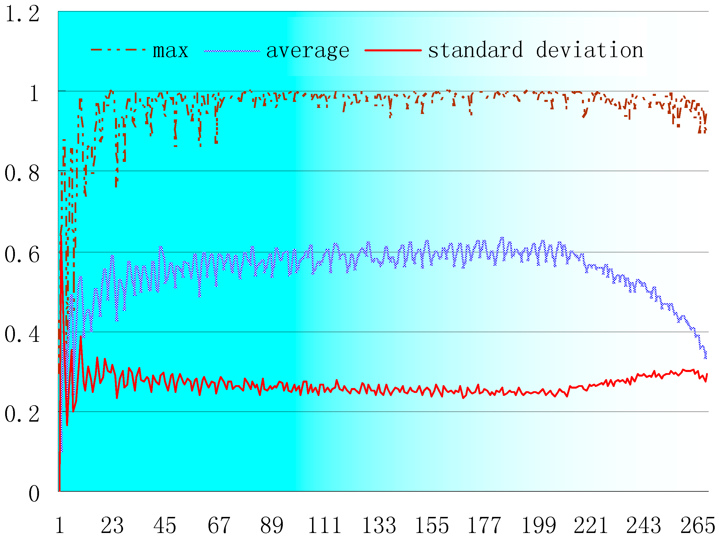
3.3. Simulation Study

Generate three points randomly in a two-dimensional plane, and divide the space using different neighborhood configurations. As is shown in Figure 10, spatial division results are closely related to the configuration of cell neighborhoods. Division results of standard Moore-type and von Neumann-types are always uncertain and not in conformity with the actual situations as a result of the two neighborhood types’ own anisotropy. Results of spatial division of the improved-type based on map algebra are consistent with the results of vector division, showing that it is a more accurate, realistic and adequate description of simulated spatial processes than the others mentioned above.

Figure 10. Comparison diagram of the simulation division results.

Figure 10. Comparison diagram of the simulation division results.

4. Research on Weighted CA Diffusion Model and Its Application

4.1. Data Sources and Illustrations

Henan province is located in the central region of China. Since the proposal of “Rise of Central China” strategy in 2005, the development and potential of Henan Province and Zhong yuan Metropolitan Area (Zhengzhou is the core of it) have become a focal point of research. Many scholars generally believe that Zhong yuan Metropolitan Area is the engine of the region’s economic and social development. Therefore, a clear understanding of the spatial pattern and development trend of the urban area in Henan province is necessary. This article selects all the cities as the research subjects to display the development of the city area in 2013.

4.2. Rule Making of CA

The link intensity between regions is directly proportional to the population and inversely proportional to the square of the distance and its expression is as follows [27,28]:

$$F_{ij}=G\frac{P_i{P}_j}{r_{ij}^2}$$

(9)

F_ij is interacting force between i, and j, G is the gravitational constant; P_i, P_j are scales of these regions, which vary in problems faced, and population scale is the common choice; r_ij is the distance between i and j.

Suppose that P_X is the scale of point X on the contour of P_i and P_j. According to the gravity model, the point X from P_i and P_j is as follows:

$$F_{iX}=G\frac{P_i{P}_X}{r_{iX}^2}, F_{jX}=G\frac{P_j{P}_X}{r_{jX}^2}$$

(10)

Because X is on the contour of urban gravity, thus F_iX = F_jX, and the distance from the point on the boundary of two cities to its corresponding city should satisfy the following formula:

$$\frac{r_{iX}}{r_{jX}}=\sqrt{\frac{P_i}{P_j}}$$

(11)

Suppose that the diffusion speeds of cells from the adjacent cities i and j are v_i and v_j, the time for the cell diffusing to the boundary is t_i and t_j and that X is a point on the contour of gravity of city i and city j, then:

$$r_{iX}=v_i{t}_i, r_{jX}=v_j{t}_j$$

(12)

Put them into Formula (11), it follows from this that:

$$\frac{v_i{t}_i}{v_j{t}_j}=\sqrt{\frac{P_i}{P_j}}$$

(13)

Because the time for the formation of the boundary of two adjacent cities is the same, that is t_i = t_j, then:

$$\frac{v_i}{v_j}=\sqrt{\frac{P_i}{P_j}}$$

(14)

Formula (14) demonstrates the main premise for determining the CA-based urban sphere of influence. Studying the patterns of urban spheres of influence must take the strength of the city into account and taking urban strength as a weight of CA diffusion makes geographic sense. P is the urban non-agricultural population and v is the diffusion step in unit time, that is, the weights W.

4.3. Mathematical Definition of Determination of CA-Based Urban Affecting Area

Definition 7. (mathematical definition and rule-making of spatial pattern formed by weighted CA diffusion): there is a two-dimensional raster space L (m × m), m × m Cells, each cell has four states: $•$ is the generator, $\nabla$ is the developed cell, − is the non-developed cell, * is the boundary cell. There are P fixed points (generators), P is 2 or greater. Suppose $Q$ = {$•$, $\nabla$, −, *}, $\left|Q\right|$ = 4, the states of cell x and its neighborhood u(x) are x^t, u(x)^t, and the state of the neighborhood is equal to $M(u{(x)}^t)=\{h\in Q|\exists y\in u(x),y^t=h\}$, $I{(x)}^t=M(u{(x)}^t)\cap${$•$, +, −, *}.

Take the neighborhood of von Neumann type, for example, and suppose the raster distance of central cell in the direction of 45 degrees is D₀:

$$D_0=\{d_t\in D_0|d_t=\frac{\sqrt{2}}{2}t,t\in N\}$$

(15)

Suppose the distance from the other raster to the generator is D₁:

$${\text{D}}_1=\text{de2}(\text{i},\text{j})={(\text{i}-1)}^2+{(\text{j}-1)}^2$$

(16)

Then, take the direction of 45 degrees as the basic distance to inspect the development of the cell center’s neighborhood.

Transition of the cell’s state at different moments has relations as follows:

$$x^{t+1}=\{\begin{array}{l}•(x^t=-)\cap I{(x)}^t\supseteq \{•\}\cap \left|{(D_0-D_1)}^{t+1}\right|>1\\ +(x^t=•)\cap I{(x)}^t\supseteq \{-\}\cup (x^t=\text{+})\\ -(x^t=-)\cap I{(x)}^t\supseteq \{-\}\\ \ast (x^t=•)\cap I{(x)}^t\subseteq \left\{\text{+}\right\}\cap \left|I{(x)}^t\right|\ge 2\cap \left|{(D_0-D_1)}^{t+1}\right|>1\cup (x^t=\ast )\end{array}$$

Transformations: transform constrain

$$\begin{array}{l}•\to +I{(x)}^t\supseteq \{-\}\\ -\to •I{(x)}^t\supseteq \{•\}\cap \left|{(D_0-D_1)}^{t+1}\right|>1\\ •\to \ast I{(x)}^t\subseteq \left\{\text{+}\right\}\cap \left|I{(x)}^t\right|\ge 2\cap \left|{(D_0-D_1)}^{t+1}\right|>1\end{array}$$

It is noteworthy that diffusion speeds of waves coming from different generators are different at the same moment because weights of different generators are not the same. Suppose the weight-vector is W = (W1, W2 ... Wp), then the time of fluctuation of each generator at each moments is in accordance with their weight.

4.4. Analysis of Result

Figure 11 displays the development of urban sphere of influence of Henan Province based on CA. Henan province is one of the birthplaces of Central Plains culture. Because of its geography, history and many other reasons, there are large numbers of intensive-distributed cities in this province. Especially, eight cities aggregate in the group with Zhengzhou at its core, and the area of this group is large. Chinese central metropolitan regions gain limited advantages from national investment and policy. In other words, plentiful resources, industrial agglomeration and superfluous government budget within the central urban places would result in disparity between the core and hinterland cities. Moreover, medium or smaller-sized cities around the provincial city greatly depend on the central cities, and are becoming new clusters of industry development with populations relocating there, as a result of economic globalization and regional integration [29]. Therefore, compared with the polarity of Zhengzhou, the urban influential regions of periphery cities decline tremendously, which leads to a “string of beads” pattern forming in this area [30]. Northern Henan, such as Xinxiang area, has a smaller number of cities characterized by aggregate development. This distribution type which has higher-grade cities intermingled with low-level cities mainly concentrates around large cities. There is potential and tendency of integrated development in this region because of their short distances from each other. In the rest of Henan, middle-sized and small cities are scattered. There is no city above the county level near another. The distance becomes an obstacle, as well as the effect of administrative boundaries, causing the single-polar development of the urban spheres of influence of Luohe, Zhoukou, Xiangcheng, and Zhumadian.

Figure 11. Sphere of influence of Henan cities in 2007.

Figure 11. Sphere of influence of Henan cities in 2007.

With the wide use of Weibo, more and more applications using Weibo data for social network analysis of network data mining are emerging. The users who are sending Weibo could be recorded with their geographical information. Using the geographic mark Weibo can find the scope and strength of human activity, which directly shows the sphere of influence of all kinds of cities. Weibo data during January 2014 to June 2014 would be used and calculated as the Weibo frequency per one kilometer, which is demonstrated in Figure 12. It is noted that cities located in Zhengzhou area are expansive from the aspect of Weibo. Around Xinxiang area there is potential and tendency of integrated development because of the short distance among them and continuous policy guidance. The spatial pattern of Weibo frequency is monopolar in Luohe-Zhoukou-Xiangcheng-Zhumadian area, which indicates single-polar development for these cities. Generally, the delineation of urban spheres of influence based on the improved CA model is reasonable and could correctly reflect the state of regional development.

Figure 12. Frequency of Weibo use in Henan.

Figure 12. Frequency of Weibo use in Henan.

5. Conclusions and Prospects

Choice of cellular neighborhood configuration has a significant impact on space division structure. There exists uncertainty in space division based on standard CA neighborhoods while the effect is not obvious and the interoperability is not strong when making improvements using dynamic transformation and complex neighborhood configurations. The improved neighborhood configuration based on map algebra ensures the accuracy of diffusion with strong isotropic characteristics. In terms of space division and the diffusion simulation, it is especially advantageous, far beyond other configurations. In order to further propose the weighted-diffusion of CA, the gravity model was applied. Then, we studied the area division and change analysis in time dimensions of urban spheres of influence of cities in Henan province, China, for example. The result reflects that CA can be reasonably applied to geosciences. On this basis, the cellular automata will make its mark in many aspects such as weighted-diffusion, analysis of the shortest path and network and so on, and the related areas are worthy of further study.

References

1. Zhou, C.H.; Sun, Z.L.; Xie, Y.C. Reasrch of Geographic Cellular Automata; Science Press: Beijing, China, 1999. [Google Scholar]
2. Neumann, J.V. The General and Logical Theory of Automata; Pergamon Press: London, UK, 1963. [Google Scholar]
3. Von Neumann, J. Theory of Self-Reproducing Automata; University of Illinois Press: Champaign, IL, USA, 1966. [Google Scholar]
4. Ulam, S. Adventures of a Mahematician; University of California Press: Oakland, CA, USA, 1991. [Google Scholar]
5. Burks, A.W. Eassys on Celualr Automata; University of Illinois Press: Champaign, IL, USA, 1970. [Google Scholar]
6. Xie, H.M. Nonlinear Scientific Series: Complexity and Dynamic System; Shanghai Science and Technology Education Press: Shanghai, China, 1994. [Google Scholar]
7. Jenertte, G.D.; Wu, J. Analysis and simulation of land-use change in the central Arizona-Phoenix region, USA. Landsc. Ecol. 2001, 16, 611–626. [Google Scholar]
8. Menard, A.; Marceau, D.J. Simulating the impact of forest management scenarios in an agricultural landscape of southern Quebec, Canada, using ageographic cellular automata. Landsc. Urban. Plan. 2007, 79, 253–265. [Google Scholar] [CrossRef]
9. Semboloni, F. The growth of an urban cluster into a dynamic self-modifying spatial pattern. Environ. Plan. B Plan. Des. 2000, 27, 549–564. [Google Scholar] [CrossRef]
10. Stevens, D.; Dragicevic, S.; Rothley, K. City: A GIS-CA modelling tool for urban planning and decision making. Environ. Model. Softw. 2007, 22, 761–773. [Google Scholar] [CrossRef]
11. Sun, T.; Wang, J. A traffic cellular automata model based on road network grids and its spatial and temporal resolution’s influences on simulation. Simul. Model. Pract. Theory 2007, 15, 864–878. [Google Scholar] [CrossRef]
12. Chen, Q.; Mynett, A.E. Effects of cells size and configuration in cellular automata based prey-predator modeling. Simul. Model. Pract. Theory 2003, 11, 609–625. [Google Scholar] [CrossRef]
13. Jantz, C.A.; Goetz, S.J. Analysis of scale dependencies in an urban land-use change model. Int. J. Geogr. Inf. Sci. 2005, 19, 217–241. [Google Scholar] [CrossRef]
14. Li, X.; Ye, J.A. Constrained Cellular Automata for Modelling Sustainable Urban Forms. J. Geogr. Sci. 1999, 54, 289–298. [Google Scholar]
15. Wu, F.; Martin, D. Urban expansion simulation of Southeast England using population surface modelling and celular automata. Environ. Plan. A 2002, 34, 1855–1876. [Google Scholar] [CrossRef]
16. Li, C.M.; Chen, J. Generation of Voronoi Diagram for Entities by Dynamic Distance Transformation. Theor. Res. 2000, 1, 6–10. [Google Scholar]
17. Hu, P.; Y, L.; Yang, C.Y.; Wu, Y.L. Map Algebra; Wuhan University Press: Wuhan, China, 2002. [Google Scholar]
18. Gu, C.; Pang, H. Study on Spatial Relations of Chinese Urban System: Gravity Model Approach. Geogr. Res. 2008, 27, 2–10. [Google Scholar]
19. Du, G.Q. Using GIS for analysis of urban system. Geo J. 2001, 52, 213–221. [Google Scholar]
20. Huff, D.L.; Lutz, J.M. Urban Spheres of Influence in Ghana. J. Dev. Areas. 1989, 23, 201–220. [Google Scholar]
21. Huff, D.L.; Lutz, J.M. Change and Continuity in the Irish Urban System, 1966–1981. Urban. Stud. 1995, 32, 155–173. [Google Scholar] [CrossRef]
22. Gold, C.M. The meaning of “neighbour”. In Theories and Methods of Spatio-Temporal Reasoning in Geographic Space; Springer-Verlag: Berlin, Germany, 1992; pp. 220–235. [Google Scholar]
23. Okabe, A.; Boots, B.; Sugihara, K.; Chiu, S.N. Spatial Tessellations, Conceptsand Applications of Voronoi Diagrams; John Wiley & Sons Ltd.: New York, NY, USA, 2000. [Google Scholar]
24. Deng, Y.; Liu, S.H.; Wang, L.; Ma, H.Q.; Wang, J.H. Field Modeling Method for Identifying Urban Spheres of Influence: A Case Study on Central China. Chin. Geogra. Sci. 2010, 20, 353–362. [Google Scholar] [CrossRef]
25. Wang, K.Y.; Deng, Y.; Sun, D.W.; Song, T. Evolution and spatial patterns of spheres of urban influence in China. Chin. Geogra. Sci. 2014, 24, 126–136. [Google Scholar] [CrossRef]
26. Wang, H.; Deng, Y.; Tian, E.Z.; Wang, K.Y. A comparative study of methods for delineating sphere of urban influence: A case study on central China. Chin. Geogra. Sci. 2014, 24, 1–12. [Google Scholar] [CrossRef]
27. Wang, X.; Wu, D.T.; Wang, H.Q. An attempt to calculate economic links between cities. Urban. Dev. 2006, 3, 55–59. [Google Scholar]
28. Reilly, W.J. Methods for the Study of Retail Relationship. Univ. Texas Bull. 1929, 2944, 29–44. [Google Scholar]
29. Carley, M. Urban Partnerships, Governance and the Regeneration of Britain’s Cities. Int. Plan. Stud. 2000, 5, 273–298. [Google Scholar] [CrossRef]
30. Huff, D.L. The Delineation of a National System of Planning Regions on the Basis of Urban Spheres of Influence. Reg. Stud. 1973, 7, 323–329. [Google Scholar]