Biomass Power Generation Industry Efficiency Evaluation in China

Abstract

In this paper, we compare the properties of the traditional additive-based data envelopment analysis (hereafter, referred to as DEA) models and propose two generalized DEA models, i.e., the big M additive-based DEA (hereafter, referred to as BMA) model and the big M additive-based super-efficiency DEA (hereafter, referred to as BMAS) model, to evaluate the performance of the biomass power plants in China in 2012. The virtues of the new models are two-fold: one is that they inherited the properties of the traditional additive-based DEA models and derived more new additive-based DEA forms; the other is that they can rank the efficient decision making units (hereafter, referred to as DMUs). Therefore, the new models have great potential to be applied in sustainable energy project evaluation. Then, we applied the two new DEA models to evaluate the performance of the biomass power plants in China and find that the efficiency of biomass power plants in the northern part of China is higher than that in the southern part of China. The only three efficient biomass power plants are all in the northern part of China. Furthermore, based on the results of the Wilcoxon-Mann-Whitney rank-sum test and the Kolmogorov-Smirnov test, there is a great technology gap between the biomass power plants in the northern part of China and those in the southern part of China.

1. Introduction

As a developing country with a huge population, China is always relatively short of energy storage. Now, with the rapid development of the economy, along with industrialization and urbanization, the energy consumption of China will increase to four billion Mtce, and the gap between energy production and consumption will reach half of the total energy volume. Meanwhile, China is still one of the few countries that rely on fossil energy, which has caused severe environmental problems. The energy shortage and defective infrastructure now is pushing China to seek out and develop substitution energies.

Being the one and only material and easily-stored renewable energy, biomass power generation is getting more and more attention globally. Till the end of 2012, the installation capacity of biomass power in the U.S. had exceeded 10,000 megawatts, and the capacity now has been planned to account for 50% of their total energy production. Furthermore, Germany aims to use biomass power to meet 16% of the whole country’s electricity demand, 10% of the heating demand and 15% of electric vehicle (hereafter referred to as EV) power.

According to the publicized the International Energy Agency (IEA) data in 2012, China has abundant biomass resources with a productivity of about five billion tons per year, and this amount ranks only next to fossil resource. Hence, China can develop biomass power. However, compared with the development of hydro, nuclear, wind and solar power, biomass power in China had not fully started until the implementation of the Renewable Energy Act in 2006. Now, the installation capacity has increased by 30% each year, and according to the Long-Term Renewable Energy Development Plan, in 2020, the expected biomass power installation capacity will be 30 GW. With the industrial plan and policy incentives, biomass power in China has entered the track of high-speed development.

Under this situation, if enough data can be collected and used to evaluate the industry efficiency quantitatively, then the assessment can provide a basis for decision making and suggest industrial or policy measurements to improve efficiency, which, in return, will accelerate the industrialization of biomass power in China and keep the development leading in the optimal direction.

2. Literature Review and Emerged Concerns

Developed countries in Europe and the U.S. started their research on biomass power in the 1970s, and the early research commonly focused on the energy conversion technology. With the subsequent development of the biomass power industry, the studies and concerns shifted to the generating cost and industry efficiency. Hooper had come up with countermeasures from the view of investment for the development of the biomass power generation industry. In the research, technology needed to be advanced, and it was the best choice to industrialize and commercialize [1]. Biomass power took off late in China, and the studies about biomass generating technology were summed up and learned. Hence, the domestic research began with focusing on the economy and industry efficiency.

After the implementation of the Renewable Energy Act, the biomass power in China entered a phase with high-speed in industrial growth. It created profitability for the biomass power generation in China and encouraged researchers to perform comprehensive assessment methods to study the industry efficiency, not only to calculate the technical efficiency, but also to evaluate the scale and overall efficiency. Along this track, Christoph and Perrels used scenario analysis and an input-output model and studied the relationship between biomass power and CO₂ emissions [2]. Klevas and Denis used DEA to analyze the technical efficiency of some common renewable technologies, including biomass technology [3,4]. Based on their methods, Peng Zhou in China meliorated the DEA model and made it suitable for overall efficiency assessment [5]. DEA methods showed their advantage in evaluating the efficiency of the biomass power generation industry, and domestic scholars started to apply them to China’s own data. Zhao chose SWOT to analyze the industry state of the biomass power generation of China and thought that the advantage lied in the increasing electricity demand and changing electricity price, yet, the industry was sensitive to local policy and the local industrial environment [6]. Kautto also compared the regional and national biomass power plan, finding that if the regional plan can cooperate with national development better, the whole biomass industry efficiency would take a step toward a higher level [7]. In all, the regional or local situation indeed impacts the industry efficiency of biomass power generation.

As for China, with multiple geographical features and an unbalanced economy, the regional difference is distinct, and the regional effect easily influences the biomass industry assessment; hence, the region needs to be considered as a key factor when performing an industry efficiency evaluation. Other than that, when Ramon used Multi-criteria data envelopment analysis model (MCDEA) to assess the efficiencies of 13 projects located in different areas, some weights of the indexes were zero [8], which made the index lose the ability to contribute to the assessment and led to the inaccuracy of the efficiency ranking. Li et al. used a unified efficiency DEA model to evaluate the performance of 24 power companies in China [9].

In terms of methodology, DEA is widely used in evaluating the performance of biomass power generation plants. DEA, first proposed by Charnes et al. in 1978, is a methodology for evaluating and measuring the relative efficiencies of a set of decision making units (DMUs) that use multiple inputs to produce multiple outputs [10]. Subsequent to that pioneering study, the research work has been mainly focused on constructing different DEA models to compensate for the disadvantage of traditional DEA models, e.g., the additive model [11], slack-based model [12,13], cross-efficiency model [14] and assurance region model [15] have been proposed to solve a variety of problems [16].

Till now, there have still been two problems concerning the application of DEA models: one is that the traditional models are unable to deal with negative or nil data, and the other is that they cannot rank the efficient DMUs. Based on this, this paper presents two new models, the big M additive-based DEA (BMA) model and big M additive-based super-efficiency DEA (BMAS) model, to solve this problem. In addition, we apply the new DEA models to evaluate the performance of biomass generation plants in China and give the relevant policies based on the result of the model.

3. Industrial Characteristics of Biomass Power Generation in China

3.1. Conservative Rising Development Tendency

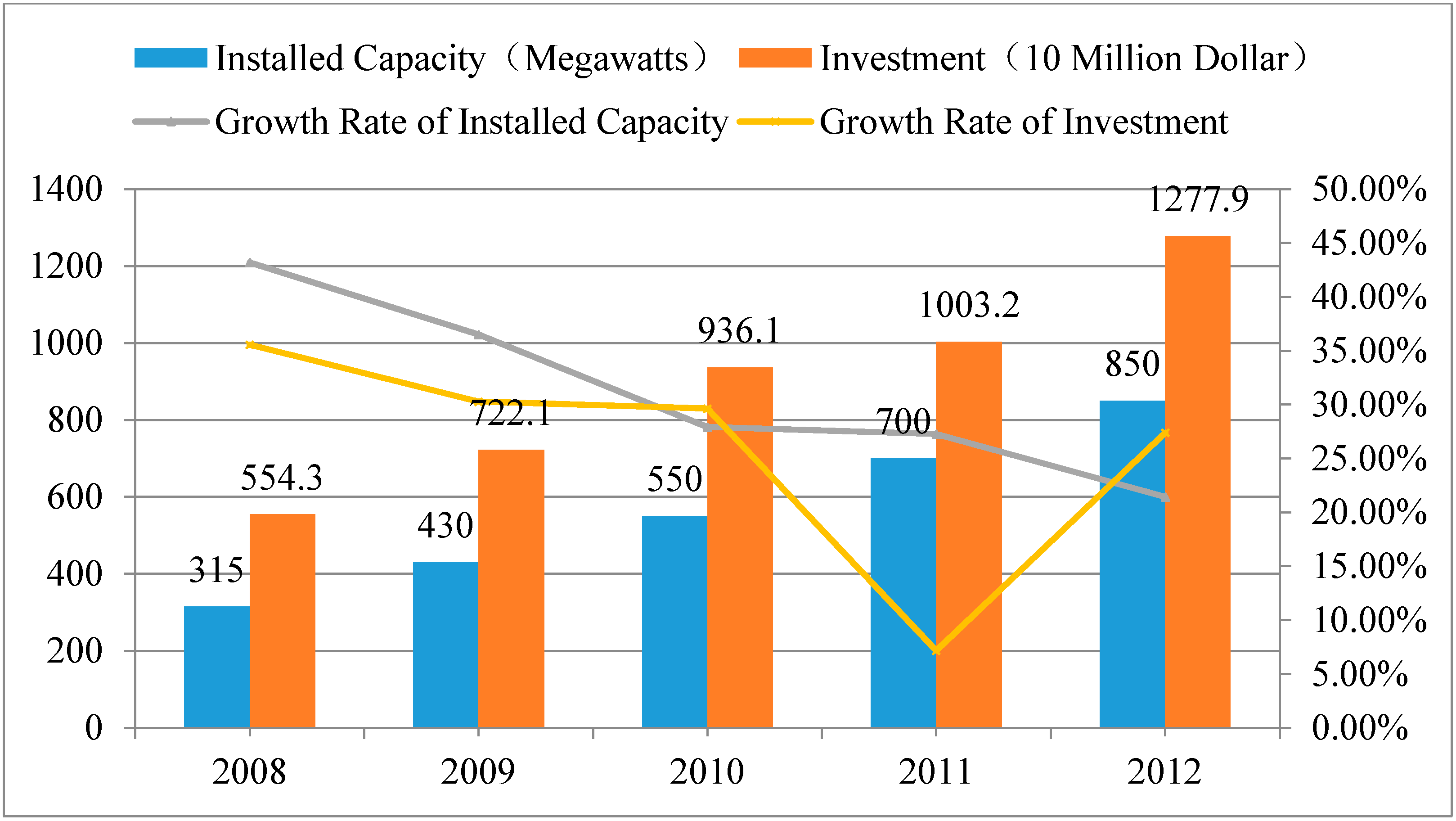
Since 2006, the biomass power generation industry has made huge progress. According to Zhao et al. [17], from 2008 to 2012, the installation capacity increased from 315 megawatts to 850 megawatts and the investment increased from 5.543 billion to 12.779 billion dollars; both of these two indicators’ average growth rate per annum reached above 20%, which is shown in Figure 1.

Figure 1. Industry scale and investment tendency chart of biomass power generation in China.

Figure 1. Industry scale and investment tendency chart of biomass power generation in China.

The average growth rate per annum of installation capacity and investment were both high during the recent past five years, but they were reducing each year, which showed that in China, the biomass power generation scale keeps growing, but the growth rate is sinking. On the one hand, this fits the growth law; on the other hand, this shows that China is developing biomass power with a positive, but conservative attitude.

According to “the 12th Five-Year Plan” and Long-Term Renewable Energy Development Plan, the Chinese government plans to develop the installation capacity of biomass power to 13 GW and invest over 90 billion RMB to achieve this goal.

3.2. Simple Impacts from the Industry Chain

In China, the industry chain of biomass power generation is simple. The up-stream companies are fuel suppliers and device manufactures, while the down-stream one is the power-grid company. Because the fuel cost accounts for almost 60% of the whole biomass power generation cost in China, the impact from the up-stream is the fuel cost. According to the IEA estimate (shown in Table 1), the potential biomass resource is abandoned; therefore, the fuel cost will not change dramatically in the near future.

Table 1. Potential biomass resource estimates in China (10⁸ Mtce).

Year		2010	2020	2030	2050
Biomass resource type	Present biomass resource	2.8	2.8	2.8	2.8
	Newly-added organic waste	0.6	1.7	2.2	2.7
	Present woodland growth	0.05	0.3	0.7	1.37
	New ground marginal product	0.05	0.3	1	2
	Total potential	3.5	5.1	6.7	8.9

Table 1. Potential biomass resource estimates in China (10⁸ Mtce).

Year		2010	2020	2030	2050
Biomass resource type	Present biomass resource	2.8	2.8	2.8	2.8
	Newly-added organic waste	0.6	1.7	2.2	2.7
	Present woodland growth	0.05	0.3	0.7	1.37
	New ground marginal product	0.05	0.3	1	2
	Total potential	3.5	5.1	6.7	8.9

As for the down-stream company, because China now practices a “full amount buy in” policy for renewable energy and biomass power does not account for a large proportion, the electricity demand fluctuation has little impact on the biomass power generation industry, and the main impact is reflected by the feed-in price. According to the regulation “Agriculture and Forestry Biomass Price Policy” from the National Development and Reform Commission of China (NDRC), the feed-in price is set to 0.75 RMB per KWh (including the tax) for the new biomass project, which has not obtained its investor through biding.

3.3. Distinct Regional Difference

It is distinctive that the biomass power generation industry in China has a regional feature. This is partly because different regions have different types of biomass resources, and this is also due to the production characteristic of different biomass resources. For example, straw burning biomass power generation plants have been built in the south of China, because that area is rich in crop resources; while in the east of China, the city area produces lots of municipal waste and so garbage power plants are built.

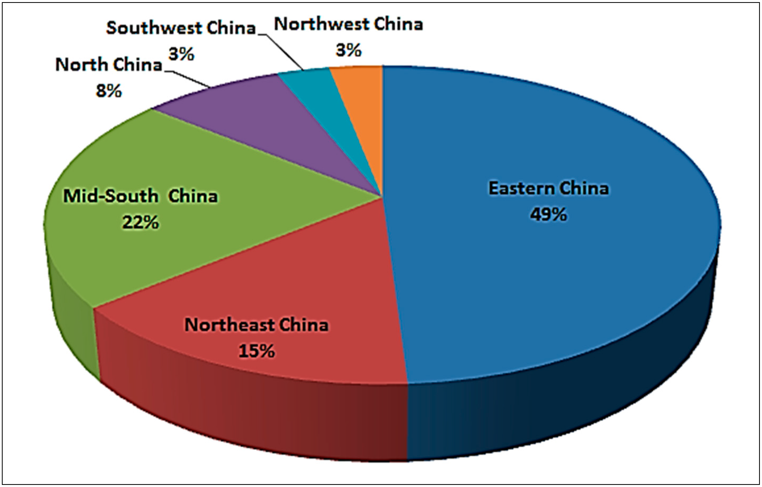
Now, China’s biomass power capacity is mainly located in eastern China and then ranks from mid-south, northeast, north, southwest to northwest China. Till the end of 2012, the biomass power installation capacity distributed in the above area is shown in Figure 2. This proportion will not change in the following years and so neither does the investment distribution.

Figure 2. Biomass power distribution in China till 2012.

Figure 2. Biomass power distribution in China till 2012.

4. Methodology

Suppose there are n units being evaluated (in short, DMUs); each DMU has m inputs and s outputs. X denotes the m × n input indicator matrix, while Y denotes the s × n output indicator matrix. That is to say, x_ij denotes the i-th input indicator of the j-th DMU, while y_rj denotes the r-th output indicator of the j-th DMU. Finally, X_j denotes the input vector of the j-th DMU, while Y_j denotes the output vector of the j-th DMU.

4.1. Drawbacks of Traditional DEA Models

The CCR model [10] and BCC model [18] are the two main traditional DEA models. Compared to the CCR model, the BCC model takes into account the factors of returns to scale; thus, here, the BCC model is selected to show the drawbacks of classical DEA models when facing negative and nil data.

The BCC linear program (LP) model and its dual model can be illustrated as follows:

$$\begin{array}{l}\text{max} {\text{μ}}^T{Y}_o+{\text{μ}}_0\\ st.\{\begin{array}{l}{\text{ω}}^T{X}_o=1,\\ {\text{μ}}^T{Y}_j-{\text{ω}}^T{X}_j\text{+}{\text{μ}}_0\le 0,j=1,\dots ,n,\\ \text{μ}\ge 0,\text{ω}\ge 0.\end{array}\end{array}$$

(1)

$$\begin{array}{l}\text{min} \text{θ}\\ st.\{\begin{array}{c}{\displaystyle \sum _{j=1}^n{\text{λ}}_j{y}_{rj}-s_r^{+}=\text{θ}{y}_{ro},r=1,\dots ,s,}\\ -{\displaystyle \sum _{j=1}^n{\text{λ}}_j{x}_{ij}-s_i^{-}=-x_{io}},i=1,\dots ,m,\\ {\displaystyle \sum _{j=1}^n{\text{λ}}_j=1},\\ {\text{λ}}_j\ge 0,s_i^{-}\ge 0,s_r^{+}\ge 0,j=1,\dots ,n.\end{array}\end{array}$$

(2)

here, ω and μ denote the weight vectors of the inputs and outputs, respectively, and “st.” denotes “subject to”. Traditional DEA models supposed that each DMU’s value is positive, which demonstrating that they are powerless when facing negative and nil data.

Lins et al. pointed out that, “In order to use the above amounts in the DEA it was necessary to alter the variables so as to avoid negative or nil values. To do so, all the cells in each column with negative or nil values were added to the lowest value in this column, with the addition of one unit” [19]. It is noted that, since the traditional DEA model does not have the translation invariance property, the method used by Lins et al. is not correct when facing negative and nil data.

4.2. Additive-Based DEA Models

In order to solve the negative data problem, many new DEA models were proposed, most of which were characterized as additive-based models, because of the translation invariance property of the additive model. The translation invariance, as is pointed out by Lovell and Pastor, is critical when the data contain zero or negative values and must be translated prior to analysis with available software packages [20]. The first additive-based DEA model, named the constant weighted additive model (CWA-DEA), was proposed by Pastor in 1994. It shared the translation invariance property with the original additive model, while neither of them was unit invariant [20]. In order to obtain a model that shared both the translation invariance and unit invariance properties, Lovell and Pastor in 1995 proposed the normalized weighted additive model (NWA-DEA), which was a great step forward in the history of additive-based DEA models [20]. They used the sample standard deviations of the output variables and the input variables, respectively, to replace the constant weight in the CWA-DEA model, and they pointed out that any first order dispersion measures can also be used to normalize the input excess and output slack variables. Apart from the translation invariance and unit invariance properties, three other important properties were proposed by Cooper et al. to testify to the quality of the additive-based DEA models [21]. Furthermore, based on the five properties, Cooper et al., 1999, and Cooper et al., 2011, extended the NWA-DEA model and proposed the famous RAM and BAM models [21,22]. The five properties were:

(P1)

The optima is between 0 and 1;

(P2)

The optima is 0 when DMU_o is fully inefficient, while the optima is 1 when DMU_o is fully efficient;

(P3)

The optima is well defined and unit invariant;

(P4)

The optima is strongly monotonic;

(P5)

The optima is translation invariant.

According to Cooper et al., 1999, the “strong monotonicity” property is described as follows: holding all other inputs and outputs constant, an increase in any of its inputs will increase the inefficiency score for an inefficient DMUo. The same is true for a decrease in any of its outputs [21].

Table 2 describes whether current DEA models satisfy these five properties. According to Lovell and Pastor, 1994, the CCR model and the normalized weighted CCR model were not translation invariant, while the BCC model and the normalized BCC model are translation invariant in a limited sense, being invariant with respect to the translation of inputs or outputs, but not both. The radial component of the efficiency measure obtained from the BCC model and the CCR model is unit invariant, but the slack component is not [20]. The additive model can only measure the inefficiencies of the DMUs, and the optima are not between 0 and 1. With respect to P4, it is obvious that only the RAM model satisfied the strongly monotonic property, while the others are all monotonic.

Table 2. Comparisons of traditional DEA models on the five properties.

Model	P1	P2	P3	P4	P5
CCR	Yes	Yes	Partially Units Invariance	Monotonic	NO
Normalized weighted CCR	Yes	Yes	Units Invariance	Monotonic	NO
BCC	Yes	Yes	Partially Units Invariance	Monotonic	Partially Translation Invariance
Normalized weighted BCC	Yes	Yes	Units Invariance	Monotonic	Partially Translation Invariance
Additive model	No	No	No	Monotonic	Yes
Normalized weighted Additive Model	No	No	Units Invariance	Monotonic	Yes
SBM	Yes	Yes	Yes	Monotonic	Yes
RAM	Yes	Yes	Yes	Strongly Monotonic	Yes
BAM	Yes	Yes	Yes	Monotonic	Yes

Table 2. Comparisons of traditional DEA models on the five properties.

Model	P1	P2	P3	P4	P5
CCR	Yes	Yes	Partially Units Invariance	Monotonic	NO
Normalized weighted CCR	Yes	Yes	Units Invariance	Monotonic	NO
BCC	Yes	Yes	Partially Units Invariance	Monotonic	Partially Translation Invariance
Normalized weighted BCC	Yes	Yes	Units Invariance	Monotonic	Partially Translation Invariance
Additive model	No	No	No	Monotonic	Yes
Normalized weighted Additive Model	No	No	Units Invariance	Monotonic	Yes
SBM	Yes	Yes	Yes	Monotonic	Yes
RAM	Yes	Yes	Yes	Strongly Monotonic	Yes
BAM	Yes	Yes	Yes	Monotonic	Yes

4.3. Generalized Additive-Based DEA Model-BMA Model

Based on the previous research, we proposed a generalized additive-based DEA model, which was called the big M additive-based DEA model. We here not only show that the previous additive-based DEA models were the particular form of the big M additive-based DEA model, but also show that other different forms of additive-based models can be derived from the big M additive-based DEA model.

Consider the following model:

$$\begin{array}{l}\text{θ}\hspace{0.17em}=\hspace{0.17em}\text{min}\left[1-\frac{{\displaystyle \sum _{r=1}^s\frac{s_r^{+}}{\text{Ψ}(\text{Ω})}}+{\displaystyle \sum _{i=1}^m\frac{s_i^{-}}{\text{Φ}(\text{Ω})}}}{M}\right]\\ st.\{\begin{array}{c}{\displaystyle \sum _{j=1}^n{\text{λ}}_j{y}_{rj}-s_r^{+}=y_{ro},r\hspace{0.17em}=\hspace{0.17em}1,\dots ,s},\\ -{\displaystyle \sum _{j=1}^n{\text{λ}}_j{x}_{ij}-s_i^{-}\hspace{0.17em}=\hspace{0.17em}-x_{io}},i\hspace{0.17em}=\hspace{0.17em}1,\dots ,m,\\ {\displaystyle \sum _{j=1}^n{\text{λ}}_j\hspace{0.17em}=\hspace{0.17em}1},\\ {\text{λ}}_j\ge 0,s_i^{-}\ge 0,s_r^{+}\ge 0,j\hspace{0.17em}=\hspace{0.17em}1,\dots ,n.\end{array}\end{array}$$

(3)

here, Ω denotes the sample space, Ψ(Ω) and Φ(Ω) are non-zero mappings from the sample space to ℝ with homogeneous properties, i.e., θΦ(Ω) = Φ(θΩ), θΨ(Ω) = Ψ(θΩ), θ ϵ ℝ, and big M is a large real number. The following theorem motivates the proposition of the homogeneity property of the mappings Ψ(Ω) and Φ(Ω).

Theorem 1: (Lovell and Pastor [20]) In an additive DEA model, scaling an input (output) by multiplying it by a constant α > 0 is equivalent to leaving the input (output) unscaled and multiplying the corresponding input excess (output slack) variable in the objective function by the same constant.

Therefore, Model (3) is unit invariant if and only if Ψ(Ω) and Φ(Ω) satisfy the homogeneity property. In this sense, the additive-based DEA models mentioned above are only the particular form of the big M additive-based DEA model. Obviously, Model (3) can be transformed into the additive model, if we set Ψ(Ω) = 1, Φ(Ω) = 1 and M = 1. It can be transformed into the normalized weighted additive model when we set Ψ(Ω)_r = σ_r, Φ(Ω)_i = σ_i and M = 1. Here, σ_r, σ_i denote the sample standard deviation of the r-th output variable and the i-th input variable. It can be transformed into the SBM model when we set Ψ(Ω)_r = s·y_ro, Φ(Ω)_i = m·x_io and M = 1. It can be transformed into the RAM model when we set Ψ(Ω)_r = ${\text{R}}_r^{+}$, Φ(Ω)_i = ${\text{R}}_i^{-}$ and M = (m + s), where $R_i^{-}={\overline{x}}_i-{\underset{¯}{x}}_i$ with ${\overline{x}}_i=\text{max}\{x_{ij},j=1,\dots ,n\}$, ${\underset{¯}{x}}_i=\text{min}\{x_{ij},j=1,\dots ,n\}$ and $R_r^{+}={\overline{y}}_r-{\underset{¯}{y}}_r$ with ${\overline{y}}_r=\text{max}\{y_{rj},j=1,\dots ,n\}$, ${\underset{¯}{y}}_r=\text{min}\{y_{rj},j=1,\dots ,n\}$. It can be transformed into the BAM model when we set Ψ(Ω)_r = ${\text{U}}_{ro}^{+}$, Φ(Ω) = ${\text{U}}_{io}^{-}$ and M = (m + s), where $L_{io}^{-}=x_{io}-{\underset{¯}{x}}_i$ and $U_{ro}^{+}={\overline{y}}_r-y_{ro}$. Moreover, it is obvious that the mappings Ψ(Ω) and Φ(Ω) control the unit invariance property, i.e., property (P2) and M control the properties of (P1), (P2) and (P4).

Furthermore, we can get various additive-based DEA models when we set different types of Ψ(Ω), Φ(Ω) and M. We listed several types of Ψ(Ω), Φ(Ω) and M as follows:

Case 1: p, q order geometric moment. $\text{Ψ}(\text{Ω})\hspace{0.17em}=\hspace{0.17em}{({\displaystyle \sum _{j=1}^n{y}_{rj}^p})}^{\frac{1}{p}},p=1,\dots ,\text{∞}$, and $\text{Φ}(\text{Ω})\hspace{0.17em}=\hspace{0.17em}{({\displaystyle \sum _{j=1}^n{x}_{ij}^q})}^{\frac{1}{q}},q=1,\dots ,\text{∞}$. It is noted that Ψ(Ω) = max{y_rj, j = 1, …, n} and Φ(Ω) = max{x_ij, j = 1, …, n} when p,q = ∞.

Case 2: p, q order central moment. $\text{Ψ}(\text{Ω})\hspace{0.17em}=\hspace{0.17em}{({\displaystyle \sum _{j=1}^n{(y_{rj}-{\overline{y}}_r)}^p})}^{\frac{1}{p}},p=1,\dots ,\text{∞}$, and $\text{Φ}(\text{Ω})\hspace{0.17em}=\hspace{0.17em}{({\displaystyle \sum _{j=1}^n{(x_{ij}-{\overline{x}}_i)}^q})}^{\frac{1}{q}},q=1,\dots ,\text{∞}$, where ${\overline{x}}_i,{\overline{y}}_r$ denote the mean value of the i-th input and the r-th output, respectively.

Then, we researched whether the generalized additive-based DEA model satisfies the five properties mentioned above.

Theorem 2: (P1) The optimum of Model (3) is between 0 and 1 only when M is big enough.

Proof: Since whatever Ψ(Ω) and Φ(Ω) are, we could always find an M big enough, such that ${\displaystyle \sum _{r=1}^s\frac{s_r^{+}}{\text{Ψ}\left(\text{Ω}\right)}}+{\displaystyle \sum _{i=1}^m\frac{s_i^{-}}{\text{Φ}\left(\text{Ω}\right)}}=\hspace{0.17em}{\displaystyle \sum _{r=1}^s\frac{{\displaystyle \sum _{j=1}^n{\lambda }_j{y}_{rj}}-y_{ro}}{\text{Ψ}\left(\text{Ω}\right)}}+{\displaystyle \sum _{i=1}^m\frac{x_{io}-{\displaystyle \sum _{j=1}^n{\lambda }_j{x}_{ij}}}{\text{Φ}\left(\text{Ω}\right)}}\hspace{0.17em}\le \hspace{0.17em}M$; thus $1-\frac{{\displaystyle \sum _{r=1}^s\frac{s_r^{+}}{\text{Ψ}\left(\text{Ω}\right)}}+{\displaystyle \sum _{i=1}^m\frac{s_i^{-}}{\text{Φ}\left(\text{Ω}\right)}}}{M}\ge 0$. Furthermore, since ${\displaystyle \sum _{r=1}^s\frac{s_r^{+}}{\text{Ψ}\left(\text{Ω}\right)}}+{\displaystyle \sum _{i=1}^m\frac{s_i^{-}}{\text{Φ}\left(\text{Ω}\right)}}\ge 0$, $1-\frac{{\displaystyle \sum _{r=1}^s\frac{s_r^{+}}{\text{Ψ}\left(\text{Ω}\right)}}+{\displaystyle \sum _{i=1}^m\frac{s_i^{-}}{\text{Φ}\left(\text{Ω}\right)}}}{M}\le 1$.

Theorem 3: (P2) The optimum of Model (3) is 1 when DMU_o is fully efficient, while the optimum of Model (3) is not 0 when DMU_o is fully inefficient.

Proof: It is obvious that $s_i^{-}$, ${\text{s}}_r^{+}$ are all equal to zero when DMU_o is fully efficient; thus, the optimum is one. However, when DMU_o is fully inefficient, the optimum varies when different M are chosen.

Theorem 4: (P3) The optimum of Model (3) is well defined and unit invariant.

Proof: Based on Theorem 1, it is obvious that Model (3) is unit invariant if and only if Ψ(Ω) and Φ(Ω) satisfy the homogeneity property. Moreover, since Ψ(Ω) and Φ(Ω) are non-zero mappings, Model (3) is well defined.

With respect to (P4) and (P5), it is obvious that the optima of Model (3) is not necessarily monotonic (the proof is similar to that of (P4’) in Cooper et al., 2011, and the optimum is not monotonic when we simply choose Ψ(Ω) = x_i.), and it satisfies the translation invariance property.

4.4. BMAS Model

Since classical DEA models can only recognize the efficiency of each unit, when there are many efficient DMUs, they cannot be ranked. Classic super-efficiency DEA models can effectively solve the problem of ranking effective decision making units, but they cannot deal with the negative and nil data problem. Based on this, this paper presents the BMAS model to solve these problems.

Consider the model below:

$$\begin{array}{l}\text{θ}\hspace{0.17em}=\hspace{0.17em}\text{min}\left[1-\frac{{\displaystyle \sum _{r=1}^s\frac{s_r^{+}}{\text{Ψ}(\text{Ω})}}+{\displaystyle \sum _{i=1}^m\frac{s_i^{-}}{\text{Φ}(\text{Ω})}}}{M}\right]\\ st.\{\begin{array}{l}{\displaystyle \sum _{\begin{array}{l}j=1\\ \text{j}\ne {\text{j}}_{\text{0}}\end{array}}^n{\lambda }_j{Y}_{rj}-s_r^{+}=Y_{r{j}_0},r=1,\dots ,s，}\\ -{\displaystyle \sum _{\begin{array}{l}j=1\\ j\ne j_0\end{array}}^n{\lambda }_j{X}_{ij}-s_i^{-}=-X_{i{j}_0}},i=1,\dots ,m,\\ {\displaystyle \sum _{\begin{array}{l}j=1\\ j\ne j_0\end{array}}^n{\lambda }_j=1},\\ {\lambda }_j\ge 0,s_i^{-}\ge 0,s_r^{+}\ge 0,j=1,\dots ,n.\end{array}\end{array}$$

(4)

The difference between the BMA model and BMAS model is only in the construction of the production possibility set. The BMAS model excludes the DMU evaluated from the production possibility set and only considers the new production possibility set constructed by the remaining DMUs. Then, we could evaluate this DMU based on the new production possibility set.

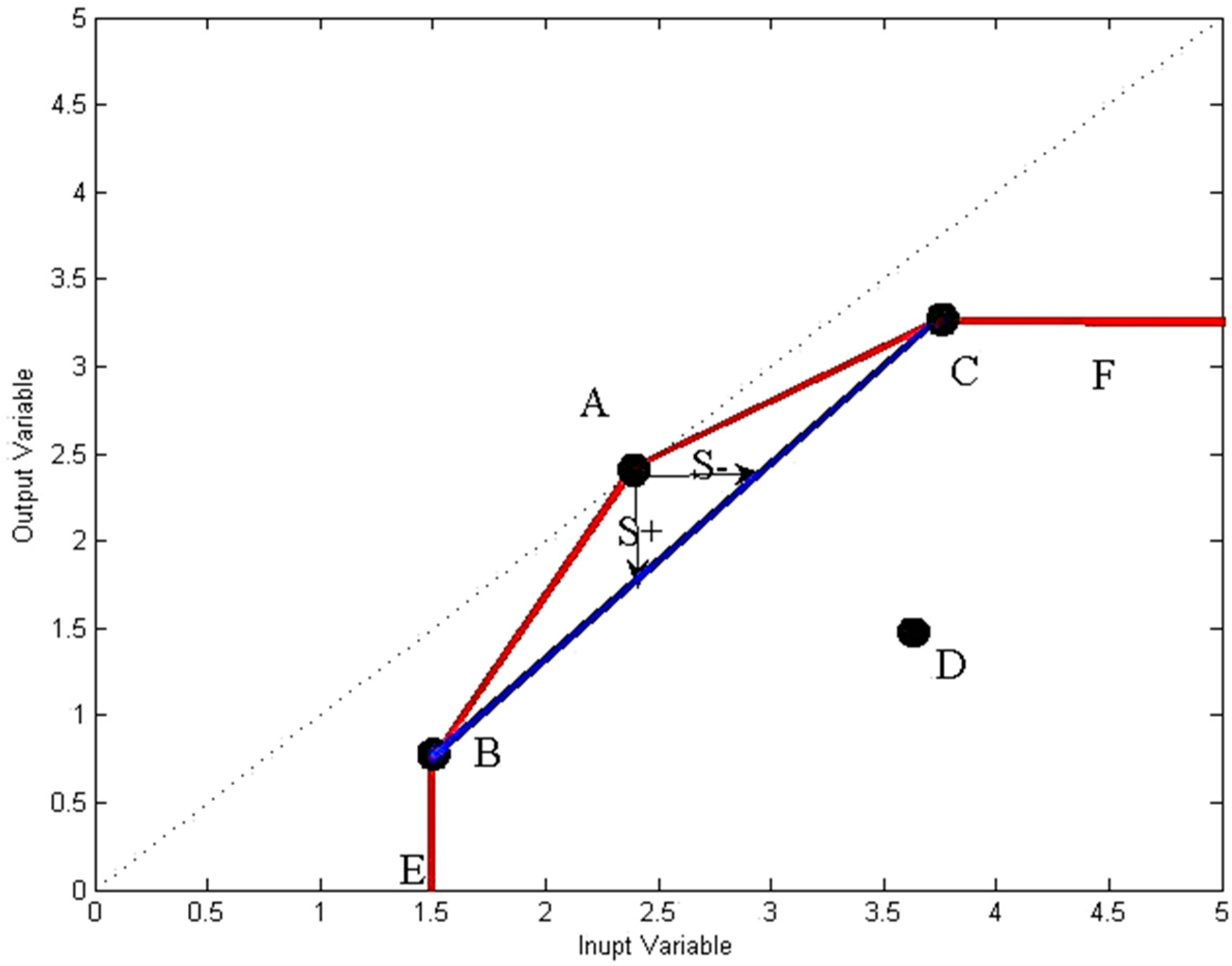
Thus, when the DMU being evaluated is efficient in the original DEA model, it would be outside of the new production possibility set which is constructed by the remaining DMUs. As a result, $s_i^{-}$, ${\text{s}}_r^{+}$ would be less than zero, so that the value of the objective function would be greater than one. In addition, since the distance between DMUs and the frontier varies from different DMUs, the efficiency would be measured by these distances. If the distance is short, the efficiency is relatively low, while if the distance is long, the efficiency is relatively high. Figure 1 shows that the production possibility set of the original DEA models (BCC) is the district constructed by EBACF, while the new production possibility set of the super-efficiency DEA models is the district constructed by EBCF. With respect to A, Figure 3 shows that $s_i^{-}$, ${\text{s}}_r^{+}$ are less than zero.

Figure 3. The improvement of inefficient DMU on the production possibility set.

Figure 3. The improvement of inefficient DMU on the production possibility set.

5. Empirical Analysis

5.1. Efficiency Analysis

In China, the efficiency of biomass power plants can be seen as the efficiency of the entire biomass generation industry. We employ the methodology in Section 4 to evaluate the efficiency of biomass power plants in China. The data consist of 11 biomass power plants in 2012 (it is noted that in China, most biomass power plants’ data are classified information and are unavailable to the public; therefore, we here only obtained the data of 11 biomass power plants by making surveys). The input variables selected are: greenhouse gases emission, investment costs, operation and maintenance costs. The output variables selected are: potential job creation and potential distributed power generation. Here, greenhouse gas emissions were calculated based on the documents of the Methods and Guidelines of Calculating the Greenhouse Gases Emissions of Chinese Power Plants. Data of investment costs, operation and maintenance costs were obtained from the financial statements of each biomass power plant. Potential job creation means the maximum amount of people who are willing to work at this biomass power plant, and these data were obtained by surveys to the 11 biomass power plants. Potential distributed power generation means the maximum power generated by this biomass power plant per year (or, in other words, power generation capacity (it is noted that the power generation capacity is not equal to the electric power production, and it is better to use the power generation capacity to evaluate the biomass power plants). Table 3 provides the description statistics of these 11 biomass power plants. We can see that the minimum value of operation and maintenance costs and the mean value of green gases emission are negative.

Table 3. Description statistics of the inputs and outputs of 11 biomass power plants in China.

Inputs/Outputs	Unit	Average	Std	Max	Min
Greenhouse Gas Emissions (I)	tCO2/GWh	−203.961	542.0662	600	−1223
O&M + CC Costs (I)	RMB/MWh	14.69	25.4917	62.53	−26.52
Investment Costs (I)	RMB/MWh	38.15727	18.70269	76	14.96
Potential Job Creation (O)	Job/TWh	7811.348	11,466.02	35,347.69	1.88
Potential Distributed Power Generation (O)	GWH/year	54,870.36	35,121.65	133,296	6833

Table 3. Description statistics of the inputs and outputs of 11 biomass power plants in China.

Inputs/Outputs	Unit	Average	Std	Max	Min
Greenhouse Gas Emissions (I)	tCO2/GWh	−203.961	542.0662	600	−1223
O&M + CC Costs (I)	RMB/MWh	14.69	25.4917	62.53	−26.52
Investment Costs (I)	RMB/MWh	38.15727	18.70269	76	14.96
Potential Job Creation (O)	Job/TWh	7811.348	11,466.02	35,347.69	1.88
Potential Distributed Power Generation (O)	GWH/year	54,870.36	35,121.65	133,296	6833

Here, we set Ψ(Ω)_r = σ_r, Φ(Ω)_i = σ_i and M equal to 1, and the BMA model was transformed as the normalized weighted additive-based model, which is proposed by Lovell and Pastor [20]. In order to compare the results of the BMA model with those of the traditional DEA models, we use the BCC model, the BMA model and the BMAS model to evaluate the performance of the biomass power plants in China.

Table 4 shows the result of the efficiencies obtained by the BCC model, the BMA model (normalized weighted additive-based model) and the BMAS model. The second column of Table 4 gives the efficiency of each biomass power plant, which is obtained from the BCC model, while the third column of Table 4 gives the efficiency of each biomass power plant, which is obtained by the BMA model. In comparison, the efficient biomass power plants whose efficiencies are equal to one are altered when using the BMA model. In specific, there are 10 efficient biomass power plants when using the BCC model to evaluate the performance of the 11 biomass power plants, and there are only three efficient power plants when using the BMA model, i.e., Jilin Changling, Neimeng Zhaoxin and Jinlin Gongzhuling. The main reason here is that the traditional DEA model does not have the translation invariance property; consequently, it will draw the wrong conclusion if all of the same indicators of the decision-making units increase a constant at the same time. It is noted that the function of the BMA model is to find out the efficient DMUs when facing the negative and nil data problem. However, the efficiency value of each DMU does not make any sense; it is altered when the value of the constant M alters. Meanwhile, since three DMUs’ efficiency reaches one, it is necessary to use the BMAS model to rank these efficient DMUs. The fourth column of Table 4 illustrates the super efficiency of the three efficient DMUs, which are Jilin Changling, Neimeng Zhaoxin and Jinlin Gongzhuling. From the fourth column of Table 4, it could be seen that the super efficiency of Jinlin Gongzhuling is the highest, which is 1.033233, while Neimeng Zhaoxin, with a super efficiency of 1.012733, comes in at second place, and Jilin Changling, with a super efficiency of 1.010540, in third place. Thus, these efficient DMUs, whose efficiencies are equal to one, could be ranked through their super efficiency. The fifth column of Table 4 illustrates the ranking order of each biomass power plant based on the BCC model, while the sixth column of Table 4 illustrates the ranking order of each biomass power plant given by the BMA model and the BMAS DEA model. In comparison, it could be found that the ranking order of most biomass power plants changes.

Table 4. Efficiency and ranking of each biomass power plant.

Biomass Power Plants	BCC Efficiency	BMA Efficiency	BMAS Efficiency	BCC Rank	BMA Rank	Location
Shangdong Pingyuan	1.00	0.882389		7	9	South
Hebei Wuqiao	1.00	0.984928		9	8	North
Hebei Yuanshi	1.00	0.981673		10	10	North
Anhui Shouxian	1.00	0.859524		11	11	South
Jilin Changling	1.00	1.000000	1.010540	6	3	North
Neimeng Zhaoxin	1.00	1.000000	1.012733	3	2	North
Hengshui Taida	1.00	0.988927		2	5	North
Jilin Gongzhuling	1.00	1.000000	1.033233	1	1	North
Dongping Guangyuan	1.00	0.887661		5	6	South
Shandong Pingquan	1.00	0.886453		8	7	South
Jiangxi Ganxian	0.331	0.888768		4	4	South

Table 4. Efficiency and ranking of each biomass power plant.

Biomass Power Plants	BCC Efficiency	BMA Efficiency	BMAS Efficiency	BCC Rank	BMA Rank	Location
Shangdong Pingyuan	1.00	0.882389		7	9	South
Hebei Wuqiao	1.00	0.984928		9	8	North
Hebei Yuanshi	1.00	0.981673		10	10	North
Anhui Shouxian	1.00	0.859524		11	11	South
Jilin Changling	1.00	1.000000	1.010540	6	3	North
Neimeng Zhaoxin	1.00	1.000000	1.012733	3	2	North
Hengshui Taida	1.00	0.988927		2	5	North
Jilin Gongzhuling	1.00	1.000000	1.033233	1	1	North
Dongping Guangyuan	1.00	0.887661		5	6	South
Shandong Pingquan	1.00	0.886453		8	7	South
Jiangxi Ganxian	0.331	0.888768		4	4	South

5.2. Group Analysis

Based on the distinct regional difference in Section 3.3, we found that the biomass power generation industry in China has a regional distribution feature, i.e., China’s biomass power capacity is mainly distributed in eastern China and then ranks from mid-south, northeast, north, southwest to northwest China. Therefore, it is necessary to analyze the regional differences of efficiency. Generally speaking, the investment in the biomass power generation industry of the southern part of China is much higher than that of the northern part. Therefore, is it true that the efficiencies of the southern part are significantly higher than those of the northern part?

Assumption: The efficiencies of the biomass power plants in the southern part of China are higher than those in the northern part of China.

In terms of location, from Table 5 we can see that there are five biomass power plants in the south part of China and six biomass power plants in the north part of China. In terms of the mean value, the efficiency of the northern group is 0.9923, a little higher than that of the southern group, indicating that, on average, the performance of the biomass power plants in the northern part of China is better than those in the southern part of China. In terms of the standard deviation, the value of the northern part is lower than that of the southern part, indicating that there is a great efficiency gap among the performance of biomass power plants in the southern part of China. It is noted that the maximum value of the efficiency in the southern part is 0.9888, indicating that the three efficient biomass power plants are all in the northern part of China.

Table 5. Description statistics of the efficiency between the northern group and southern group.

Group	Mean	Std	Max	Min
North	0.9923	0.0079	1.0000	0.9814
South	0.8009	0.0421	0.8888	0.7595

Table 5. Description statistics of the efficiency between the northern group and southern group.

Group	Mean	Std	Max	Min
North	0.9923	0.0079	1.0000	0.9814
South	0.8009	0.0421	0.8888	0.7595

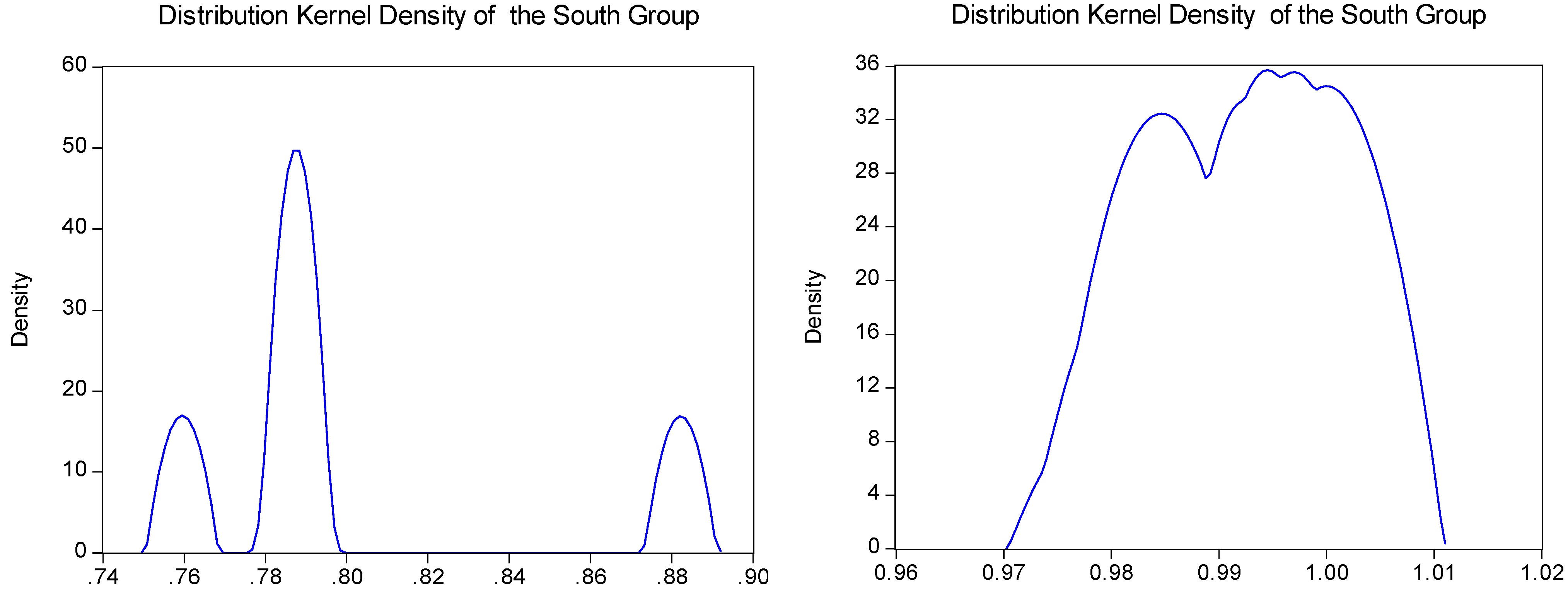
Furthermore, we conduct the Wilcoxon-Mann-Whitney rank-sum test and the Kolmogorov-Smirnov (here after referred to as K-S) test to determine the significant differences in the efficiencies between the north and south group. Figure 4 shows the distribution kernel density of the two groups, and Table 6 shows the results of the test. In terms of the Wilcoxon-Mann-Whitney rank-sum test, all null hypotheses are rejected at the 1% level, indicating that the rank differences in the efficiencies between the two groups are significant and provide support for the technological heterogeneity of the two groups. In terms of the Kolmogorov–Smirnov test, all null hypotheses are rejected at the 1% level, indicating that kernel density distribution differences exist in the efficiencies between the two groups.

Figure 4. Distribution kernel density of the two group’s efficiencies.

Figure 4. Distribution kernel density of the two group’s efficiencies.

Table 6. The Mann–Whitney rank-sum test and the Kolmogorov–Smirnov test.

Variable	Mann–Whitney U	Prob	K-S	Prob
efficiency	15	0.006	1.651	0.009

Table 6. The Mann–Whitney rank-sum test and the Kolmogorov–Smirnov test.

Variable	Mann–Whitney U	Prob	K-S	Prob
efficiency	15	0.006	1.651	0.009

From the analysis above, it is obvious that although the biomass power capacity in the southern part of China is much larger than that in the northern part, the efficiency of the northern part is significantly higher than that of the southern part. The main reason is that in the southern part, the government invested more resources (such as capital, manpower, and so on) in order to get more returns. However, the biomass power industry in China is still in the early stage, and the technology and management level are relatively lower than that of the developed countries. Therefore, there exists a large number of redundant capital investments. Therefore, the efficiencies of the southern part of China are relatively lower than those of the northern part of China. As for policy makers, they should be sensitive to the differences between the two regions. Moreover, biomass power plants should pay more attention to improving their technology level and management level when making massive investments. Finally, in order to improve the efficiencies of the southern part of China, policy makers should provide more incentives to the biomass power plants in the southern part of the China, so as to catch up with those in the northern part of China and promote the entire biomass generation industry.

6. Conclusions

In this paper, we have compared the properties of the existing additive-based DEA models and proposed two generalized additive-based models, i.e., the BMA model and the BMAS model, to evaluate the performance of the biomass power plants in China in 2012. Compared to the traditional DEA models, there are two virtues of the new models that we proposed: one is that they inherited the properties of the traditional additive-based DEA models and derived more new additive-based DEA forms; the other is that they can rank the efficient DMUs. Then, we applied the two new DEA models to the evaluation of the biomass power plants in China. The conclusions are three-folds: first, the BMA and the BMAS model have great potential to be applied in sustainable energy project evaluation; second, the efficiency of biomass power plants in the northern part of China is higher than that in the southern part of China (the only three efficient biomass power plants are all in the northern part of China); finally, based on the results of the Wilcoxon–Mann–Whitney rank-sum test and the Kolmogorov–Smirnov test, there is a great technology gap between the biomass power plants in the northern part of China and those in the southern part of China. Based on the results of the model, policy makers should provide more incentives to the biomass power plants in the southern part of the China, so as to catch up with those in the northern part of China and promote the entire biomass generation industry.

References

1. Hooper, R.; Li, J. Summary of the factors critical to the commercial application of bioenergy technologies. Biomass Bioenerg. 1996, 11, 469–474. [Google Scholar] [CrossRef]
2. Weber, C.; Perrels, A. Modelling lifestyle effects on energy demand and related emissions. Energ. Policy 2000, 28, 549–566. [Google Scholar] [CrossRef]
3. Klevas, V.; Streimikiene, D.; Grikstaite, R. Sustainable energy in Baltic States. Energ. Policy 2007, 35, 76–90. [Google Scholar] [CrossRef]
4. St. Denis, G.; Parker, P. Community energy planning in Canada: The role of renewable energy. Renew. Sustain. Energ. Rev. 2009, 13, 2088–2095. [Google Scholar] [CrossRef]
5. Zhou, P.; Ang, B.W.; Wang, H. Energy and CO2 emission performance in electricity generation: A non-radial directional distance function approach. Eur. J. Oper. Res. 2012, 221, 625–635. [Google Scholar] [CrossRef]
6. Zhao, Z.Y.; Yan, H. Assessment of the biomass power generation industry in China. Renew. Energ. 2012, 37, 53–60. [Google Scholar] [CrossRef]
7. Kautto, N.; Peck, P. Regional biomass planning—Helping to realise national renewable energy goals? Renew. Energ. 2012, 46, 23–30. [Google Scholar] [CrossRef]
8. San Cristóbal, J.R. A multi criteria data envelopment analysis model to evaluate the efficiency of the Renewable Energy technologies. Renew. Energ. 2011, 36, 2742–2746. [Google Scholar] [CrossRef]
9. Li, J.; Li, J.; Zheng, F. Unified Efficiency Measurement of Electric Power Supply Companies in China. Sustainability 2014, 6, 779–793. [Google Scholar] [CrossRef]
10. Charnes, A.; Cooper, W.W.; Rhodes, E. Measuring the efficiency of decision making units. Eur. J. Oper. Res. 1978, 2, 429–444. [Google Scholar] [CrossRef]
11. Ali, A.I.; Seiford, L.M. The Mathematical Programming Approach to Efficiency Analysis. In The Measurement of Productive Efficiency: Techniques and Applications; Fried, H.O., Schmidt, S.S., Eds.; Oxford University Press: London, UK, 1993; pp. 120–159. [Google Scholar]
12. Du, J.; Liang, L.; Zhu, J. A slacks-based measure of super-efficiency in data envelopment analysis: A comment. Eur. J. Oper. Res. 2010, 204, 694–697. [Google Scholar] [CrossRef]
13. Tone, K. A slacks-based measure of efficiency in data envelopment analysis. Eur. J. Oper. Res. 2001, 130, 498–509. [Google Scholar] [CrossRef]
14. Oral, M.; Kettani, O.; Lang, P. A methodology for collective evaluation and selection of industrial R&D projects. Manag. Sci. 1991, 37, 871–885. [Google Scholar] [CrossRef]
15. Thompson, R.G.; Langemeier, L.N.; Lee, C.T.; Lee, E. The role of multiplier bounds in efficiency analysis with application to Kansas farming. J. Econom. 1990, 46, 93–108. [Google Scholar] [CrossRef]
16. Liu, J.S.; Lu, L.Y.Y.; Lu, W.M.; Lin, B.Y.J. A survey of DEA applications. Omega 2013, 41, 893–902. [Google Scholar] [CrossRef]
17. Xingang, Z.; Zhongfu, T.; Pingkuo, L. Development goal of 30 GW for China’s biomass power generation: Will it be achieved? Renew. Sustain. Energ. Rev. 2013, 25, 310–317. [Google Scholar] [CrossRef]
18. Banker, R.D.; Charnes, A.; Cooper, W.W. Some Models for Estimating Technical and Scale Inefficiencies in Data Envelopment Analysis. Manag. Sci. 1984, 30, 1078–1092. [Google Scholar] [CrossRef]
19. Lins, M.E.; Oliveira, L.B.; Da Silva, A.C.M.; Rosa, L.P. Performance assessment of Alternative Energy Resources in Brazilian power sector using Data Envelopment Analysis. Renew. Sustain. Energ. Rev. 2012, 16, 898–903. [Google Scholar] [CrossRef]
20. Lovell, C.A.K.; Pastor, J.T. Units invariant and translation invariant DEA models. Oper. Res. Lett. 1995, 18, 147–151. [Google Scholar] [CrossRef]
21. Cooper, W.; Park, K.; Pastor, J. RAM: A Range Adjusted Measure of Inefficiency for Use with Additive Models, and Relations to Other Models and Measures in DEA. J. Product. Anal. 1999, 11, 5–42. [Google Scholar] [CrossRef]
22. Cooper, W.W.; Pastor, J.T.; Borras, F.; Aparicio, J. BAM: A bounded adjusted measure of efficiency for use with bounded additive models. J. Product. Anal. 2011, 35, 85–94. [Google Scholar] [CrossRef]