Research on the HDPE Membrane Leakage Location Using the Electrode Power Supply Mode Outside a Landfill Site

Abstract

To ensure the sustainable development of the surrounding environment and the sustainable operation of landfills, detecting landfill leakage is of great significance. In landfills lacking a leakage monitoring system, the inability to detect and locate damaged High-Density Polyethylene (HDPE) membranes can lead to the contamination of soil and groundwater by landfill leachate. To address this issue, this study proposes a resistivity tomography inversion model based on the external-electrode power supply mode. Utilizing the resistivity difference between the leakage zone and the surrounding soil, electrodes are arranged symmetrically for both power supply and measurement. Upon applying direct current (DC) excitation, potential data are collected, with the finite volume method employed for inversion and the Gauss–Newton method integrated with an adaptive particle swarm optimization algorithm for parameter fitting. Experimental results show that the combined algorithm provides better clarity in edge recognition of low-resistance models compared with single algorithms. The maximum deviation between inferred leakage coordinates and the actual location is 10.1 cm, while the minimum deviation is 6.4 cm, satisfying engineering requirements. This method can effectively locate point sources and line sources, providing an accurate solution for subsequent leakage point filling and improving repair efficiency.

1. Introduction

Solid waste management is crucial for global environmental governance [1,2]. Sanitary landfill, a common solid waste treatment method, produces a large amount of landfill leachate during operation. Prior to operation, anti-leakage layers at the bottom and slope are essential protective barriers [3,4]. The installation of the impermeable layer, a key landfill construction task, often employs HDPE (High-Density Polyethylene) membranes as the main material. During operation, HDPE membranes may leak due to sharp foreign substances in the drainage layer or leachate corrosion [5]. In order to prevent leachate from contaminating groundwater and soil, extend the sustainable operation time of landfills, and maintain the sustainable development of the surrounding environment, it is crucial to detect the leakage of High-Density Polyethylene (HDPE) membranes. This lays the foundation for subsequent plugging of the leakage points by injecting cement through boreholes [6,7].

The main methods for detecting landfill leakage during the current operational period include the direct current method [8,9,10], transmission line method [11,12,13], and stress wave method [14,15,16]. DC electromagnetic detection requires pre burying electrodes and continuous manual measurement, resulting in low efficiency. The transmission line method pre-lays conductive fibers under the HDPE membrane and uses endpoints for AC power supply and response analysis. It analyzes the terminal load’s amplitude and phase frequency characteristics to study leachate-induced changes in interline propagation and characteristic impedance, thus detecting and identifying the leachate area. The stress wave method requires preplacing vibration sensors to collect stress waves from membrane rupture. It uses wave velocity inversion for 3D ranging to locate leaks. But wave velocity calibration is affected by medium nonuniformity, and the rupture signal is weak, making detection difficult. Currently, methods such as the direct current (DC) method, transmission line method, and stress wave method require pre-installation of monitoring systems, limiting their application to newly constructed landfills. And because it needs to be pre-buried under the landfill membrane, it is vulnerable to corrosion by leachate or extrusion by the HDPE membrane. Therefore, locating leakage points in landfills that lack a monitoring system remains a key challenge. This study addresses this issue by proposing a resistivity tomography inversion model adopting an external-electrode power supply mode. This model, which does not rely on pre-installed systems, can be applied to existing landfills for real-time leakage detection. Not only does this method offer high positioning accuracy, but it also accommodates various leakage shapes.

The resistivity method is a subsurface detection approach that exploits the resistivity differences between subsurface media. In 1984, J. J. Sweeney inferred groundwater-related information using dipole–dipole electrodes [17]. In 1997, Binley et al. suggested applying this method for detecting minor leaks in insulating materials [18]. In 2000, Aristodemo et al. used the resistivity method to monitor contaminant transport in landfills [19]. In 2003, Binley et al. verified the use of electrode arrays for detecting leaks in landfill liners [20]. In 2010, Resurs R. used resistivity and induced polarization (IP) responses to measure seepage [21]. In 2016, Abdullahi developed inversion models for delineating buried waste [22]. In 2019, Akintorinwa O. J. detected potential variations within the subsurface [23]. Generally, the resistivity method measures the potential within the surveyed area by sending an excitation current. Soil resistivity is influenced by factors such as pore space [24]. It indirectly infers the resistivity of the underground medium through the study of surface potential differences to detect underground targets. Conventional methods typically depend on two-dimensional resistivity inversion to identify leakage areas but fail to pinpoint the leakage points. In this study, leveraging the high-resistance property of the HDPE membrane, electrodes are deployed beneath the membrane outside the landfill. The medium is electro permeated, and off-site data are collected for inversion imaging. The Variable Particle Swarm Algorithm and the Gaussian–Newton method are combined for model parameter fitting. This enables the analysis of resistivity differences, determination of low-resistance abnormal areas, and location of leakage points in the HDPE membrane, effectively discerning between point-source and line-source leaks.

The research hypothesis is that based on this model and method, it is possible to effectively identify low-resistance abnormal areas and accurately determine the leakage location of the HDPE membrane. In the subsequent research, for the detection principle part, the method of using resistivity differences for leakage detection based on this model will be elaborated in detail; when establishing the potential distribution model under the membrane, relevant equations are solved and boundary conditions are set to obtain the potential distribution under the membrane to provide a basis for leakage location; in the parameter fitting part, the combination of the above two algorithms is used to optimize model parameters; in the model verification and experiment part, the effectiveness of the model and method is verified by comparing the imaging results of different algorithms and actual positioning experiments.

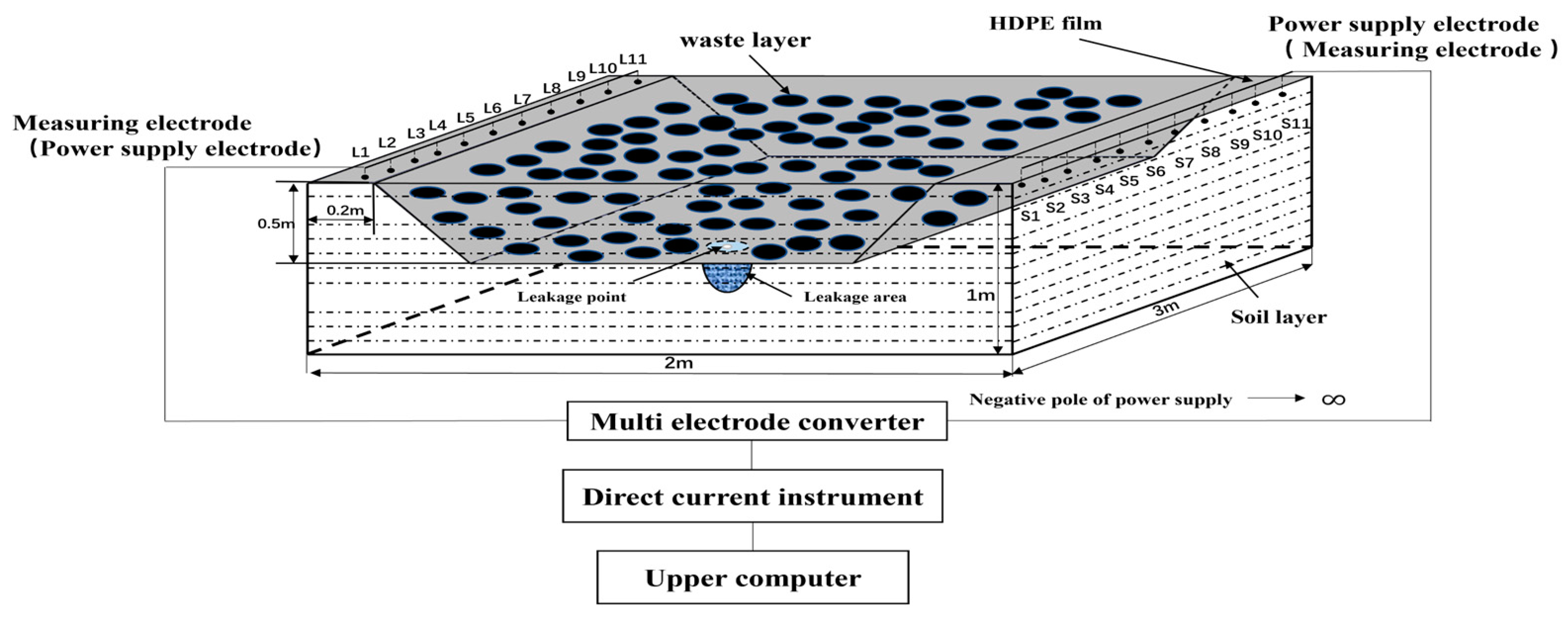
2. Principle of Detection

A location model that uses the electrode power supply mode outside the landfill is based on the resistivity anomaly of the leachate–soil mixture and the high-resistance characteristics of the HDPE (High-Density Polyethylene) membrane. When the HDPE membrane at the bottom of the waste landfill site leaks, landfill leachate seeps into the soil layer, leading to changes in parameters such as pH value, moisture content, and porosity. The soil near the leakage site shows low-resistance anomalies due to the rise in moisture content and the reduction in porosity, and the low-resistance abnormal area is more obvious when it is close to the position of the leakage point. Electrical resistivity tomography is utilized to detect areas of abnormal resistivity in the soil layer and locate the HDPE membrane leakage site. The detection principle is illustrated in Figure 1. The proposed resistivity tomography inversion model uses external-electrode power supply to measure potential beneath the HDPE membrane in landfill sites. The core idea of the method is to exploit the resistivity differences between the leakage zone and the surrounding soil. Direct electrical current is applied to the electrodes, and the potential data are collected for inversion imaging. To improve inversion accuracy, this study combines the Gauss–Newton method and an adaptive particle swarm optimization (APSO) algorithm. The Gauss–Newton method performs local optimization, while the PSO algorithm provides an effective global search for the initial model, reducing dependency on the initial setup. This hybrid algorithm allows for precise identification of low-resistance anomalies, facilitating accurate leakage point localization.

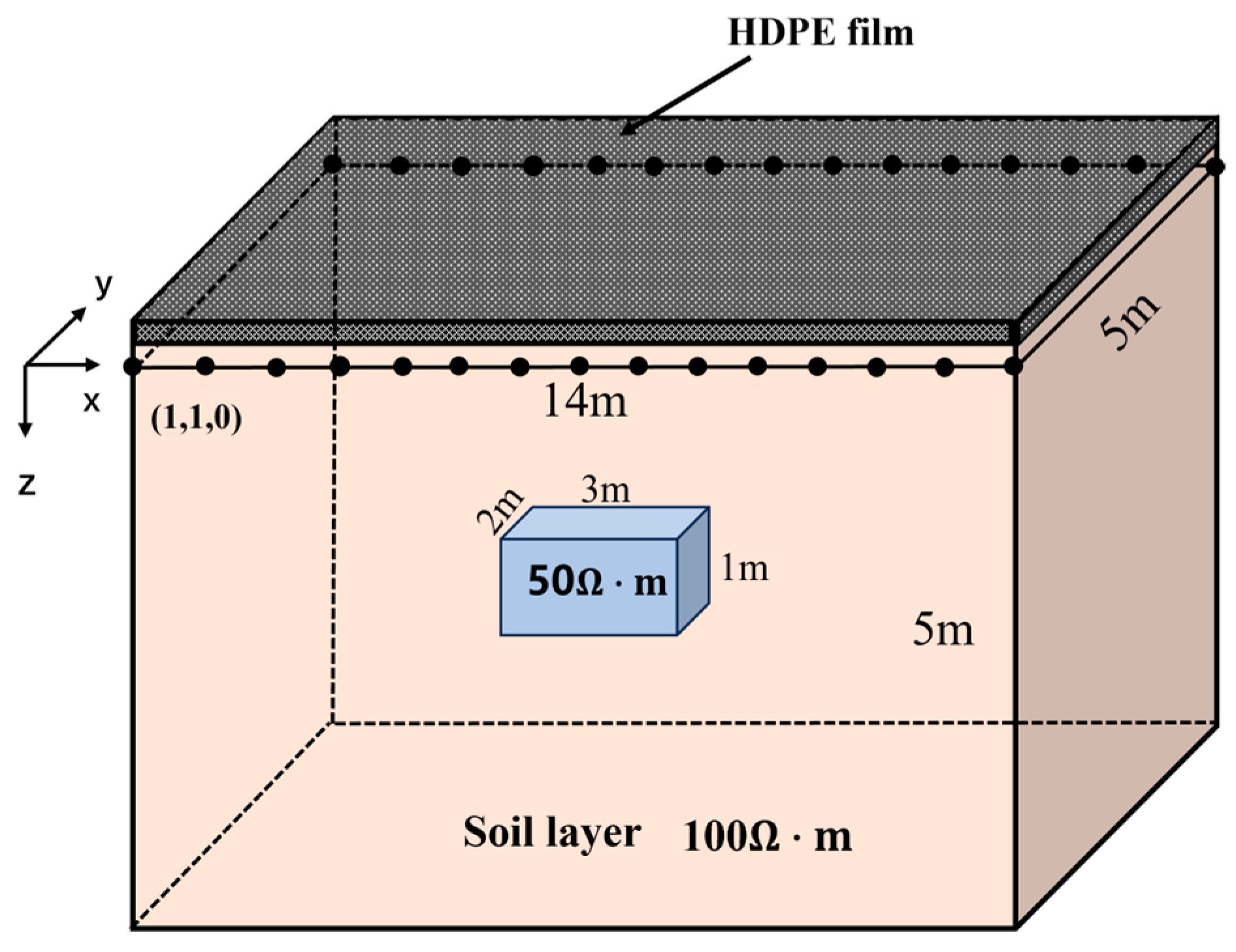
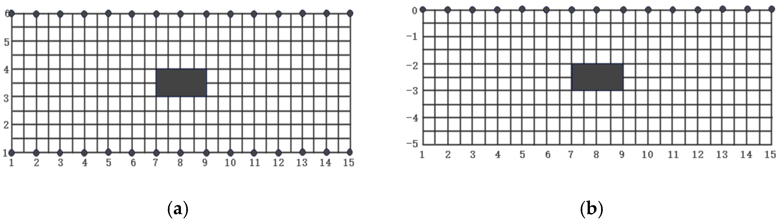
3. Potential Distribution Model Under the Membrane

The bottom reservoir and slopes of the landfill site require anti-seepage treatment, and the resistivity of the HDPE membrane is approximately $1\times {10}^{17}\Omega ·\mathrm{m}$ [3]. At the interface of the upper surface of the HDPE membrane and the drainage layer composed of sand and gravel, the current density will not change significantly. The current density experiences a distortion at the interface of the lower surface of the HDPE membrane and the soil, and it rapidly decreases after passing through the HDPE membrane. The electric field energy is mainly concentrated in the soil layer beneath the HDPE membrane, where the embedded field source is located, as illustrated in Figure 2.

Under the influence of the HDPE membrane, the boundary conditions of the electric field that is beneath the membrane are satisfied.

$$\mathrm{n}·J=0$$

(1)

In Formula (1), $\mathrm{n}$ is a normal unit vector; $J$ represents the current density, ${\mathrm{A}/\mathrm{m}}^2$.

The potential distribution at any point in the medium beneath the membrane can be described by the steady current field generated by a point current source; the computation of electric potential in space satisfies the Poisson equation:

$$\nabla ·[1/\rho (x,y,z)\nabla U(x,y,z)]=-I\delta (x-{\mathrm{x}}_0)\delta (y-{\mathrm{y}}_0)\delta (z-{\mathrm{z}}_0)$$

(2)

In Formula (2), $\rho$ represents resistivity, $\Omega ·\mathrm{m}$; $U$ represents the electrical potential, $\mathrm{V}$; $\delta$ is a Dirac function; $I$ represents the current intensity, A; ${(\mathrm{x}}_0{,\mathrm{y}}_0{,\mathrm{z}}_0)$ represents the point power supply location, m; $(x,y,z)$ represents any arbitrary location, m.

The distribution of electric fields beneath the membrane satisfies the following governing equation:

$$\left\{\begin{array}{l}\nabla J=Q\\ E=-\nabla v\\ J=(1/\rho (x,y,z))E+J_m\end{array}\right.$$

(3)

In Formula (3), $\nabla$ represents the gradient symbol; $Q$ represents the total amount of electric charge, C; $E$ represents the electric field strength, $\mathrm{V}/\mathrm{m}$; $J_m$ represents the displacement current density, ${\mathrm{A}/\mathrm{m}}^2$; $\rho$ represents resistivity, $\Omega ·\mathrm{m}$; $v$ represents the electric potential, $\mathrm{V}$.

The HDPE membrane boundary ${\Gamma }_s$ satisfies the second type of boundary conditions, and the normal current density is 0:

$${\left.{\displaystyle \frac{\partial u}{\partial n}}\right|}_{{\Gamma }_s}=0$$

(4)

According to the current continuity at the interface between different soil layers,

$${\rho }_1{\displaystyle \frac{\partial u_1}{\partial n}}={\rho }_2{\displaystyle \frac{\partial u_2}{\partial n}}$$

(5)

At the infinite boundary ${\Gamma }_{\infty }$, the third type of mixed boundary conditions is satisfied:

$${\displaystyle \frac{\partial u(x,y,z)}{\partial n}}+{\displaystyle \frac{\cos \theta }{r}}u(x,y,z)=0\in {\Gamma }_{\infty }$$

(6)

In Formulas (4)–(6): $n$ represents the coordinate variable in the normal direction of the boundary ${\Gamma }_{\infty }$ at infinity; $r$ represents the distance from the observation point to the point power source, m; $u$ represents the potential at the observation point, V; $\theta$ is the inclination of the line connecting the observation point and the point current source with respect to the normal direction.

While satisfying the potential differential equation, by defining the boundary conditions and solving the boundary value problem, a mathematical model of the potential distribution beneath the membrane can be obtained, which can be simplified to Equation (7).

$$\left\{\begin{array}{l}\left\{\nabla ·[1/\rho (x,y,z)\nabla U(x,y,z)]=-I\delta (x-{\mathrm{x}}_0)\right.\delta (y-{\mathrm{y}}_0)\delta (z-{\mathrm{z}}_0)\\ {\left.{\displaystyle \frac{\partial u}{\partial n}}\right|}_{{\Gamma }_s}=0,(x,y,z)\in {\Gamma }_s\\ {\displaystyle \frac{\partial u(x,y,z)}{\partial n}}+{\displaystyle \frac{\cos \theta }{r}}u(x,y,z)=0,(x,y,z)\in {\Gamma }_{\infty }\end{array}\right.$$

(7)

Formula (1) defines the relationship between the normal unit vector and the current density at the interface between the HDPE membrane and the soil, ensuring the current continuity at the interface. Formula (4) indicates that the normal current density at the boundary of the HDPE membrane is 0 due to the high-resistance characteristic of the HDPE membrane that prevents the current from passing through the membrane. Formula (5) adopts the third kind of mixed boundary condition at the infinite boundary, considering factors such as the distance from the observation point to the point power source, the potential, and the included angle between the line connecting the two and the normal direction of the boundary, making the model more consistent with the actual physical scenario. By setting these boundary conditions, the range of the electric field beneath the membrane can be accurately defined, providing necessary constraints for the subsequent solution of the potential distribution.

4. Establishment of HDPE Membrane Leakage Location Model

In the presence of the point-source electric field beneath the sloped membrane, the potential expression for any point in the medium beneath the membrane, except the point where the point source is located, is as follows:

$$U_0={\displaystyle \frac{I{\rho }_1}{4\pi R}}$$

(8)

In Formula (8), $U_0$ represents the potential of an arbitrary point, $\mathrm{V}$; ${\rho }_1$ represents the soil resistivity, $(\Omega ·\mathrm{m})$; $R$ represents the spatial distance between any point and the point power source, m; $I$ represents the current intensity, A.

Assuming the presence of a leakage area with resistivity ${\rho }_2$ beneath the HDPE membrane, the potential at any point within the leakage area is as follows:

$$U=U_0+U_1$$

(9)

In Formula (9), $U$ represents the overall potential, V; $U_1$ represents an abnormal potential, V.

In Figure 3, A is the power supply electrode for the slope, M and N represent the measurement points of the slope electrodes; $R_M$ and $R_N$ represent the distances from AM and AN, respectively; $r_M$ and $r_N$ represent the distances between OM and ON, respectively; ${\theta }_M$ is represented as $\angle AOM$; ${\theta }_N$ is represented as $\angle AON$. The leakage area has an irregular shape, taking the center of the inscribed circle within the irregular shape as the geometric origin point O, and the radius is a; d represents the distance from the power supply electrode to the geometric center of the leakage, O.

The anomalous potential generated at an arbitrary point within the leakage region satisfies the Laplace equation:

$${\displaystyle \frac{\partial }{\partial \mathrm{a}}}({\mathrm{a}}^2{\displaystyle \frac{\partial U_1}{\partial \mathrm{a}}})+{\displaystyle \frac{1}{\sin \theta }}{\displaystyle \frac{\partial }{\partial \theta }}(\sin \theta {\displaystyle \frac{\partial U_1}{\partial \theta }})=0$$

(10)

In Formula (10), $\theta$ represents the angle between the line connecting any point within the leakage area and point O and the z-axis. By combining boundary conditions (1), (4), and (5), we can derive the following:

$$U_1={\displaystyle \frac{I{\rho }_1}{4\pi }}{\displaystyle \sum _{n=0}^{\infty }[n({\rho }_1-{\rho }_2)]/[n{\rho }_1+(n+1){\rho }_2]}{P}_n(\cos \theta )/(d^{n+1}{a}^{n+1})$$

(11)

In Formula (11), $p_n(\cos \theta )$ is represented as a Legendre function.

Substituting Equation (10) into Equation (8) results in the potential at any point within the leakage region. According to the apparent resistivity Formula (11), the expression for the apparent resistivity at any point within the sub-membrane space has been derived:

$${\rho }_s^{AMN}=K_{MN}{\displaystyle \frac{\Delta U_{MN}}{I}}$$

(12)

$${\rho }_s^{AMN}={\rho }_1\left\{1+{\displaystyle \frac{R_M{R}_N}{R_N-R_M}}\times {\displaystyle \sum _{n=0}^{\infty }{\mu }_n\frac{a^{2n+1}}{d^{n+1}}\left[\frac{P_n(\cos {\theta }_M)}{r_M^{n+1}}-\frac{P_n(\cos {\theta }_N)}{r_N^{n+1}}\right]}\right\}$$

(13)

In Formulas (12) and (13), ${\mu }_n=[n({\rho }_1-{\rho }_2)]/[n{\rho }_1+(n+1){\rho }_2]$; ${\rho }_s^{AMN}$ represents the apparent resistivity; $K_{AMN}$ represents the device coefficient; $\Delta U_{MN}$ represents the potential difference between measurement points M and N; $I$ represents the intensity of the supply current.

Assuming the number of boundary measurement data points is N, the number of nodes in the inversion model is M, observational data are denoted as Data $d={\left[d_1,d_2,···,d_N\right]}^{\mathrm{T}}$, and the model parameter vector is denoted as $m={\left[m_1,m_2,···,m_M\right]}^{\mathrm{T}}$. To visualize the distribution of resistivity within the detection area, the detection region is initially divided into a grid model. A numerical simulation is performed on the grid model to obtain the corresponding theoretical data. Then, the theoretical data are compared with the observed data. If there is a discrepancy, the model is modified accordingly. Ultimately, a grid parameter model consistent with the observed data is obtained. Then, construct a fitting objective function:

$${\rm P}(m)={{\rm P}}_d(m)+{{\rm P}}_m(m)$$

(14)

In Formula (14), ${{\rm P}}_d(m)$ represents the data item, and ${{\rm P}}_m(m)$ is a model item.

The detection area beneath the landfill site is divided into a three-dimensional grid of $N_x\times N_y\times N_z$ dimensions; after comprehensively considering the calculation accuracy and efficiency, a grid node spacing of 0.5 m was finally selected. This configuration ensures that the potential distribution characteristics of the medium can be accurately captured while maintaining an acceptable calculation time. In the x, y, and z directions, the spacing between grid nodes is set to 0.5 m. The corresponding grid size is 30 × 10 × 10, thus forming a computational domain consisting of 3000 grid nodes. Such a grid setting not only ensures the calculation accuracy but also takes into account the calculation efficiency and can effectively simulate the potential distribution of the medium beneath the membrane. The structure employing a unit-centered approach is used to discretize the detection region [25] (Figure 4).

The potential data are collected by the measurement electrode $d={(u_1,u_2,u_3,···,u_n)}^{\mathrm{T}}$, which represents the quantity of data collected. It satisfies the Formula (2) [26]:

Using this method, the results of potential distribution under the membrane can be obtained, and then the formulas for the abnormal potential and apparent resistivity are derived. After discretization, Formula (15) is obtained:

$$Au=\mathbf{q}$$

(15)

In Formula (15), A is a forward-dispersive operator, u represents the discrete potential matrix, and q represents the point-source location matrix. Given A and q, the conjugate gradient method is employed to solve the numerical solution of the potential distribution beneath the membrane that satisfies the partial differential equation. The solution vector is updated iteratively until the convergence condition is met.

Establish initial model parameters $m={\left({\rho }_1,{\rho }_2,{\rho }_3,\cdots {\rho }_{\mathrm{s}}\right)}^{\mathrm{T}}$ and obtain the theoretical Electrical Resistivity $d\left(m\right)$; $s$ represents the number of grids involved in the inversion; by using the least squares smoothing objective function, the model parameters are fitted and approximated to the measurement data and are represented as follows:

$${\rm P}(m)={\displaystyle \frac{1}{2}}{‖W_d(d(m)-d_{ost})‖}^2+{\displaystyle \frac{\beta }{2}}{‖W_m(m-m_{ref})‖}^2$$

(16)

In Formula (16), $d_{ost}$ represents the observed apparent resistivity, $d(m)$ represents the theoretical apparent resistivity obtained from the numerical simulation of the initial model, $m$ represents the given model, $m_{ref}$ is the reference model, $\beta$ represents the smoothing factor, $W_d$ represents the weight coefficient matrix, and $W_m$ represents the model weight.

During the fitting process, the model parameters iteratively solve for the target function to minimize the objective function ${\rm P}(m)$. In the iterative process, the modification of model parameters, denoted by $\Delta m$, is conducted according to Equation (18):

$$(J^T{W}_d^{\mathrm{T}}{W}_{m}J+\beta {W_m}^{\mathrm{T}}{W}_m)·\Delta m=-(J^{\mathrm{T}}(d(m)-d_{ost})+\beta {W_m}^{\mathrm{T}}{W}_m(m-m_{ref}))$$

(17)

In Formula (17), $J=\partial d(m)/\partial (m)$ represents the Jacobian matrix.

When the objective function ${\rm P}(m)$ is minimized, in the inverse model, the model parameters achieve the minimum fitting degree with the measurement data under the smooth constraint. Compute the square root of the apparent resistivity matrix (RMS) to determine whether the inversion termination condition has been met. The expression is as follows:

$$rms=\sqrt{{\displaystyle \frac{{(d_{ost}-d(m))}^{\mathrm{T}}(d_{ost}-d(m))}{N}}}$$

(18)

In Formula (18), N represents the number of measurement data points used in the measurement process. When the square root of the fitting result of the apparent resistivity matrix meets the fitting accuracy requirement, the resistivity model is output.

5. Parameter Fitting of HDPE Membrane Leakage Localization Model

5.1. Improving the Gauss–Newton Method

To address the problems existing in model parameter fitting (such as the traditional method’s heavy dependence on the initial model and the tendency to fall into local optimal solutions when dealing with nonlinear problems, resulting in low parameter fitting accuracy and consequently affecting the accuracy of HDPE membrane leakage localization), this study improves the Gauss–Newton method. The improved method reduces computational memory and time consumption and increases iterative calculation speed by introducing an approximate Hessian matrix and combining the conjugate gradient method to solve the iterative equation.

The fitting objective function ${\rm P}(m)$ of Formula (17) is subjected to a second-order Taylor–Lagrange expansion at $m_0$; at both ends, simultaneously take the first derivative of $m$, and the iterative equation is obtained by solving $\partial {\rm P}(m)/\partial m=0$:

$$\left[H+\beta {\nabla }_m^2{{\rm P}}_m(m)\right]\Delta m=-\left[{(W_{d}J)}^{\mathrm{T}}{W}_d\left[d(m)-d_{ost}\right]+\beta {\nabla }_m{{\rm P}}_m(m)\right]$$

(19)

In Formula (19), $\Delta m$ is the modification amount for the model, $H\approx {(W_{d}J)}^{\mathrm{T}}{W}_{d}J$ denotes an approximate Heisenberg matrix with data-weighted terms, and $J$ is a partial derivative matrix of size N × M. Each element is represented by an expression:

$$J_{ij}={\displaystyle \frac{\partial (m_i)}{\partial m_j}},i=1,2,···,N;j=1,2,···,M$$

(20)

When optimizing the objective function using the Gauss–Newton method, it is necessary to constantly compute the inverse of the Hessian matrix throughout the iterative process. For uneven soils, the dominant elements on the main diagonal of the Hessian matrix are dominant, and an approximate Hessian matrix is employed in place of the original Hessian matrix [27]. Thus, the iterative formula for Equation (19) can be modified to the following:

$$\Delta m=-{\left[\mathrm{diag}(H)+\beta {\nabla }_m^2{{\rm P}}_m(m)\right]}^{-1}\left[{(W_{d}J)}^{\mathrm{T}}{W}_d\left[d(m)-d_{ost}\right]+\beta {\nabla }_m{{\rm P}}_m(m)\right]$$

(21)

In Formula (21), diag denotes the diagonal elements.

In the Gauss–Newton method, to reduce the computational memory and time required to solve Equation (21) and store the sensitivity matrix and Hessian matrix, the conjugate gradient (CG) method is employed to iteratively solve Equation (22). The multiplication of the Jacobian matrix or its transpose with an arbitrary one-dimensional vector J meets the requirements of numerical forward modeling, effectively accelerating the computational speed of inversion [28].

After obtaining $\Delta m$ through the conjugate gradient method, the model modification amount for each iteration of the Gauss–Newton method is obtained using linear search, with the update formula being the following:

$$m_{k+1}=m_k+\alpha \Delta m$$

(22)

In Formula (22), $\alpha$ denotes the model update step size. The Wolfe–Powell criterion is employed to perform an imprecise linear search and determine the updated step size. This criterion encompasses the sufficient descent condition and the curvature condition, and the corresponding formula is as follows:

$$\begin{array}{l}{\rm P}(m_k+{\alpha }_k{p}_k)\le {\rm P}(m_k)+c_1{\alpha }_k\nabla {\rm P}{(m_k)}^{\mathrm{T}}{p}_k\\ \nabla {\rm P}{(m_k+{\alpha }_k{p}_k)}^{\mathrm{T}}{p}_k\ge c_2\nabla {\rm P}{(m_k)}^{\mathrm{T}}{p}_k\end{array}$$

(23)

In Formula (23), $m_k$ represents the model parameters for the Kth iteration; ${\alpha }_k$ represents the iterative step size; $p_k$ denotes the search direction; $c_1$ and $c_2$ are constants; $c_1={10}^{-4}$, and $c_2=0.9$ [29].

The steps to fit the parameters of a positioning model using the Gauss–Newton method combined with the conjugate gradient method:

Step 1: given the initial model $m_0$, the referencing model is $m_{ref}$, the regularization parameter is $\beta$, and the model weight is $W_m$;

Step 2: calculate the difference between theoretical data from numerical simulations and observed data: $\Delta d=d_{ost}-d(m)$; calculate $r_0=g_k$; $g_k=-\left[{(W_{d}J)}^{\mathrm{T}}{W}_d\left[d(m)-d_{ost}\right]+\beta {\nabla }_m{{\rm P}}_m(m)\right]$;

Step 3: starting the conjugate gradient iterative method, the initial value $\Delta m$ = 0, $p_0=r_0$, and $i=1,2,···,N_{\max }$;

Step 4: calculate $H_k\approx {(W_{d}J)}^{\mathrm{T}}{W}_{d}J$ and obtain $H_k{p}_i$;

Step 5: calculate $t_i=(r_i^{T}r)/(p_i^{T}H{p}_i)$ and $\Delta m_{i+1}=m_i+t_i{p}_i$;

Step 6: calculate $r_{i+1}=r_i-t_i{H}_k{p}_i$ and ${\kappa }_i=(r_{i+1}^{\mathrm{T}}{r}_{i+1})/(r_i{r}_i^{\mathrm{T}})$;

Step 7: calculate $p_{i+1}=r_{i+1}+{\kappa }_i{p}_i$;

Step 8: determine the direction of the Gauss–Newton method $\Delta m_k$;

Step 9: starting from $\Delta m_k$, perform a one-dimensional search along direction $\Delta m_k$, and according to the Wolfe–Powell criterion, determine the optimal step size ${\alpha }_k$ and update the Model $m_{k+1}=m_k+{\alpha }_k\Delta m_k$;

Step 10: determine the loop condition rms < $\epsilon$, and output the optimal inverse model $m_k$; otherwise, set k = k + 1 and proceed to step 2 for another iteration.

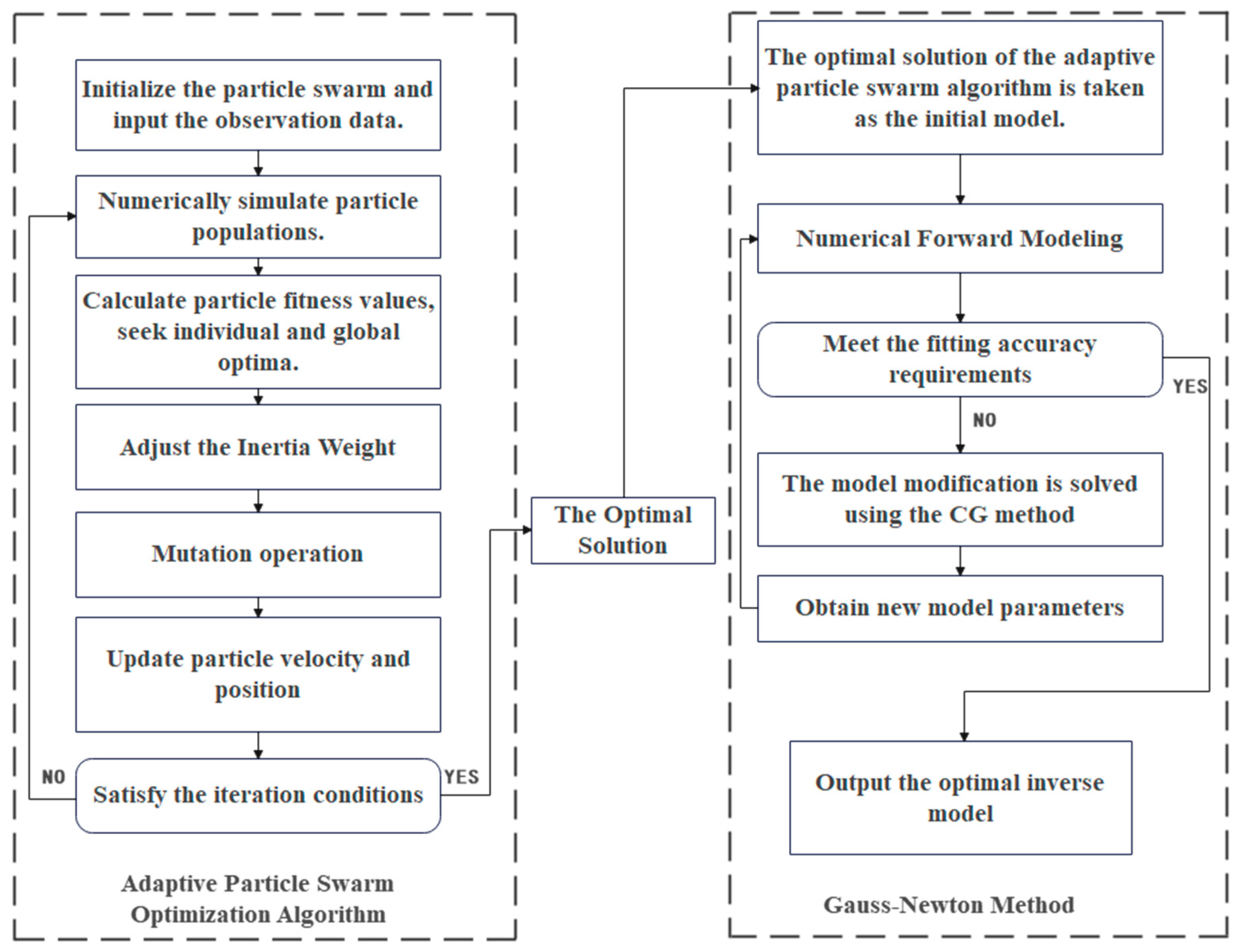
5.2. The Adaptive Particle Swarm Optimization Algorithm Is Combined with the Gaussian–Newton Method to Fit Model Parameters

Although the improved Gauss–Newton method has advantages in local search, it is still affected by the initial model. At present, nonlinear inversion based on linearization and iteration dominates due to its high convergence rate and good results [30,31,32]. However, due to the nonlinearity of soil resistivity data, truncation errors and non-uniqueness may occur during the linearization process. Moreover, the quality of conventional inversion often depends on the initial model, and an unreasonable initial model may lead to a locally optimal inversion [33,34].

In this study, a method integrating the improved Gauss–Newton method and the APSO algorithm was designed. The former utilizes its efficient local search ability to finely optimize the initial model. The latter replaces the fixed inertia weight with an adaptive weight. APSO enhances its global search ability through an adaptive weight, while GN (Gauss–Newton method) makes use of local gradient information to finely optimize the initial model generated by APSO.

The fitting procedure of the adaptive mutation particle swarm optimization algorithm integrated with the Gauss–Newton algorithm is as follows:

Step 1: initialize the particle swarm by setting the initial position and velocity of the particles, corresponding to the ith initial model of the Gauss–Newton method. Initialize the population size, individual learning factor $c_1$, and social learning factor $c_2$;

Step 2: based on the current position of the particle, a numerical simulation is conducted on the inversion model to obtain the theoretical apparent resistivity value;

Step 3: the fitness value of a particle is calculated, and the adaptive value determines the optimization approximation effect during the iterative process. In this study, the least square’s objective function with smooth constraints is employed to compute the particle’s fitness value, with the Formula (15) [35];

Step 4: based on the initial fitness values of the particles, the individual extreme value $g_{best}$ of the particles and the population extreme value $G_{best}$ are obtained [36];

$$G_i=\left\{\begin{array}{cc}{G}_{\max }-{{\rm P}}_i,& {{\rm P}}_i\le G_{\max }\\ \hfill 0,& {{\rm P}}_i\ge G_{\max }\end{array}\right.,i=1,2,···,N_{ran}$$

(24)

Step 5: using adaptive weights to implement the updating and adjustment of particle velocity and position, the formula is as follows:

$$\gamma =\left\{\begin{array}{ll}\hfill {\gamma }_{\min }-{\displaystyle \frac{({\gamma }_{\max }-{\gamma }_{\min })·(f_i-f_{\min })}{f_{avg}-f_{\min }}}\hfill & \hfill f_i\ge f_{avg}\hfill \\ \hfill {\gamma }_{\max }\hfill & \hfill f_i<f_{avg}\hfill \end{array}\right.$$

(25)

In Formula (25), ${\gamma }_{\min }$ represents the minimum value of the weight, take 0.4; ${\gamma }_{\max }$ represents the maximum weight value, take 0.9; $f_i$ represents the fitness value of the ith particle; $f_{\min }$ represents the minimum fitness value of a particle; $f_{avg}$ represents the average fitness value of the particles;

Step 6: calculate the probability of mutation $p_m$; the computational formula is as follows:

$$P_m={\displaystyle \frac{1}{N}}{\displaystyle \sum _{i=1}^N\left|\frac{f_i-f_{avg}}{f_{\max }-f_{\min }}\right|}·{\displaystyle \frac{1}{e^{\mathrm{d}(1+\frac{t}{t_{\max }})}}}$$

(26)

In Formula (26), N represents the population size, t represents the current iteration count, t_max represents the maximum number of iterations, and d is a constant used to regulate the rate of mutation probability;

Step 7: in the mutation operation, particles are sorted based on their fitness values, with the n particles with the best fitness being selected. Generate n random numbers $r_i=1,2,3···n$ distributed between 0 and 1 according to the uniform distribution, if $r_i<p_m$, the particle group is deemed to have poor diversity. The Cauchy formula is employed to mutate the optimal position of the particles. The Cauchy mutation formula is as follows:

$$Cauchy=\tan (\pi \times (rand-0.5))$$

(27)

$$G_{best}=Gg\times (1+0.5\times Cauchy)$$

(28)

In Formulas (27) and (28), $Gg$ denotes a random one between the population’s optimal location and the population’s suboptimal location, $G_{best}$ represents the global optimal position, and Cauchy represents random numbers related to the Cauchy distribution;

Step 8: calculate the current fitness value of the particle and update the particle’s extreme value $g_{best}$ and the population’s extreme value $G_{best}$;

Step 9: determine whether the number of iterations meets the set requirements. If it does, exit the iteration; otherwise, proceed to step 2;

Step 10: the inversion results of the adaptive particle swarm algorithm are substituted into the Gauss–Newton method, and the steps are shown in Figure 5.

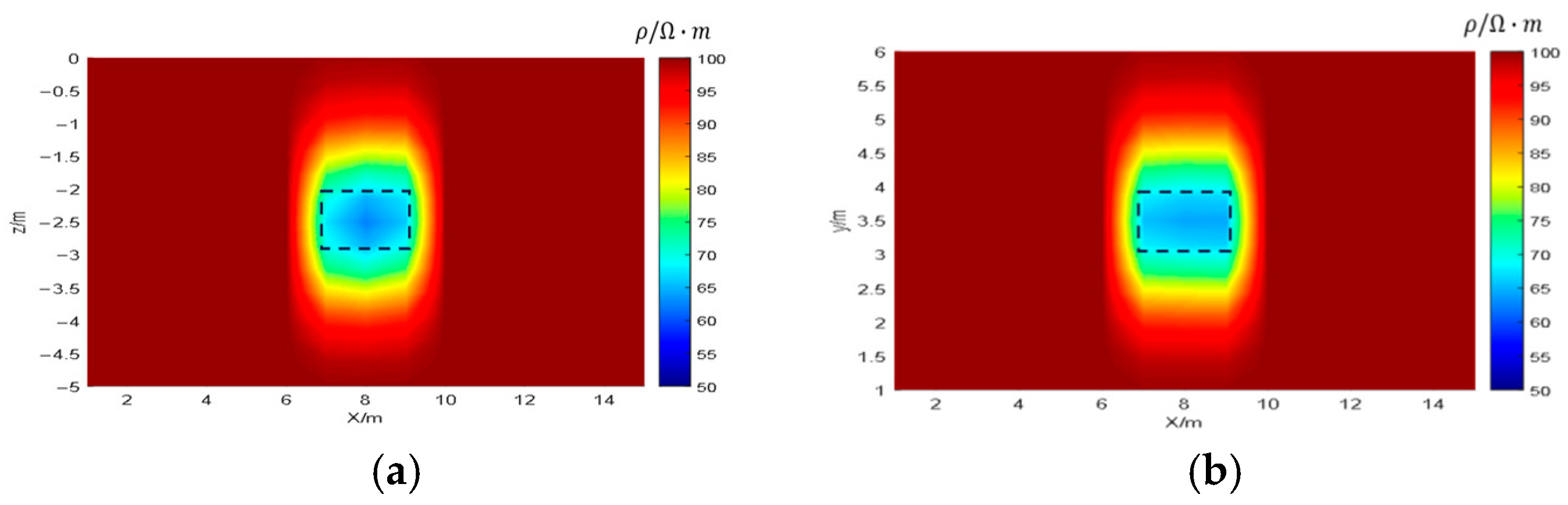
5.3. Verification of Homogeneous Medium Theory

To simplify the theoretical analysis and highlight the algorithm’s advantages, in this section, the soil layer beneath the membrane is assumed to be an isotropic medium with a uniform resistivity. The background resistivity is uniformly set at 100 $(\Omega ·\mathrm{m})$, and the resistivity of the low-resistance anomaly region is set at 50 $(\Omega ·\mathrm{m})$, and that of the HDPE membrane is 1 × 10¹⁷ $(\Omega ·\mathrm{m})$. Based on the high-resistance property of the High-Density Polyethylene (HDPE) membrane, a three-dimensional spatial model was constructed. The model has dimensions of 14 m × 5 m × 5 m, and the low-resistivity anomaly within it has dimensions of 3 m × 2 m × 1 m, with the center of the anomaly located at the coordinates (8, 3.5, −2.5), as shown in Figure 6. In accordance with the procedures described in Section 4, the inversion target area was meshed using eight-node hexahedra, as presented in Figure 7.

Using the Gauss–Newton method, APSO, and a combination of the APSO with the Gauss–Newton method, we inverted and imaged the model data, followed by comparative analysis; when using the Gauss–Newton method for inversion, the resistivity of the background area was set to 100 $(\Omega ·\mathrm{m})$. The resistivity of the abnormal area was set to 50 $(\Omega ·\mathrm{m})$, and after five iterations, the fitting accuracy rms decreased to 2% before the inversion was stopped; the imaging results are depicted in Figure 8. During the inversion process using the APSO algorithm, the population size is set to 50, and the iteration is conducted five times. The imaging results are shown in Figure 9. For the joint algorithm inversion, the imaging results are depicted in Figure 10.

For the convenience of analysis, the XOZ profile at y = 3.5 m and the XOY profile at z = −2.5 m were extracted from the 3D inversion results of three algorithms for comparative analysis. Figure 8 shows the inversion results of the Gauss–Newton method, which differ from the original model in morphology and resistivity. Figure 9 presents the results of the adaptive particle swarm algorithm, largely consistent with the original model’s outline but with resistivity differences. In contrast, Figure 10 shows the results of the joint algorithm, essentially identical to the original model in both morphology and resistivity. Figure 10 clearly shows the resistance difference contour between the background and leakage areas, effectively eliminating most interference areas, and it has high clarity in identifying the model edges. The abnormal areas are marked with dashed boxes in Figure 8, Figure 9 and Figure 10. The joint algorithm has significant advantages in the HDPE membrane leakage location model, improving location accuracy and reliability. Compared to single algorithms, it performs better in identifying low-resistance abnormal areas and determining leakage locations. In this study, the Gauss–Newton method is highly affected by the initial model, with significant fluctuations in the positioning deviation of different leakage points. Although the APSO algorithm can conduct a certain global search, its positioning accuracy can be improved. The joint algorithm combines their advantages by using the global-search ability of the APSO algorithm to obtain a better initial model and then refining it locally with the Gauss–Newton method to make the positioning result more stable and accurate. This is in line with our expected research results, which validates the research method’s effectiveness and indicates the joint algorithm has high practical value in HDPE membrane leakage location applications.

The variation of Rms during the inversion process with respect to the inversion algebra is illustrated in Figure 11. As illustrated in Figure 11, during the entire inversion process, RMS decreases from an initial value of 137.59 $(\Omega ·\mathrm{m})$ to 4.32 $(\Omega ·\mathrm{m})$. In the particle swarm optimization (the first five iterations), RMS decreases from 137.59 $(\Omega ·\mathrm{m})$ to 44.65 $(\Omega ·\mathrm{m})$, indicating a relatively rapid and monotonous descending trend. However, the transition is relatively smooth during the third to fifth iterations. In the Gauss–Newton method inversion phase (the latter five iterations), RMS decreases from 44.65 $(\Omega ·\mathrm{m})$ to 4.32 $(\Omega ·\mathrm{m})$. After a smooth decrease, RMS experiences a significant reduction, and the inversion further converges.

6. Simulation and Location Testing of Leachate Transport

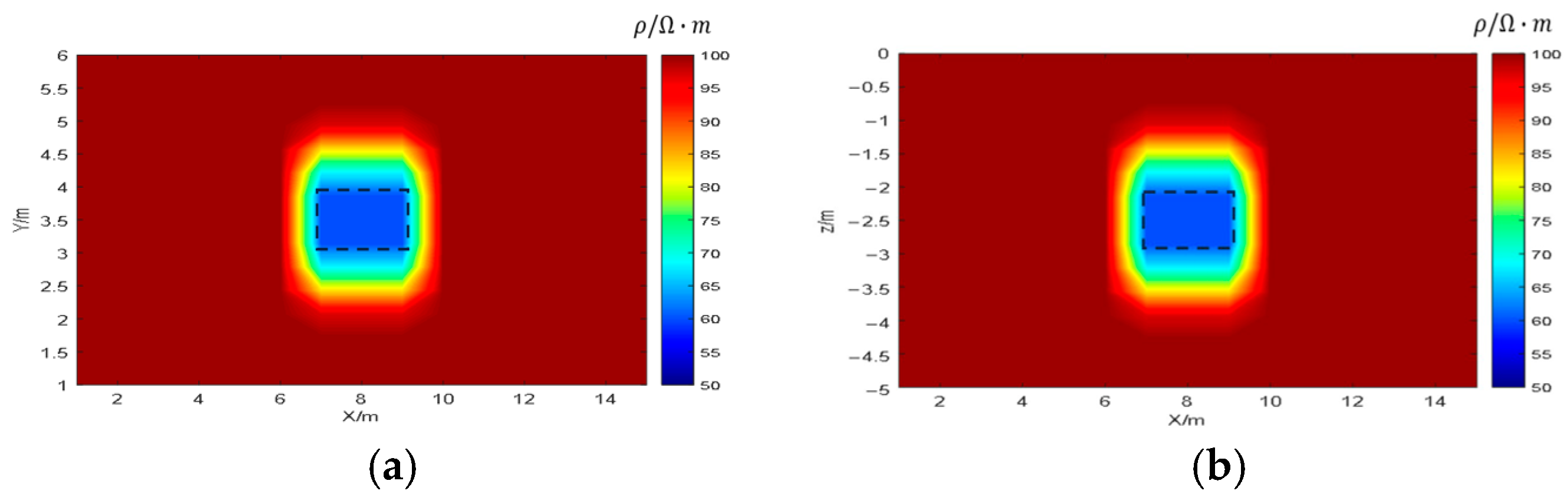
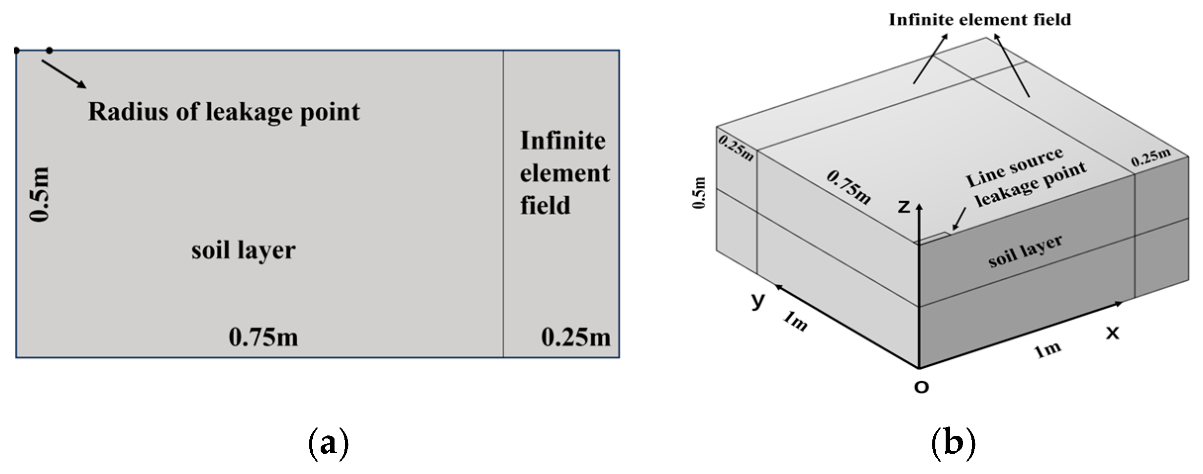
6.1. The Shape of HDPE Membrane Leak Points and Simulation of Leachate Transport

The HDPE membrane is affected by various factors during operation, with common shapes including circular point-source leakage points and linear line-source leakage points. Local water detention will occur at the leakage location during leakage when the generated leachate amount is greater than the infiltration capacity of the soil. Therefore, the flow of leachate in the soil layer belongs to saturated–unsaturated variable-saturation seepage flow. Since the drainage pipe is laid in the pebble layer, it can be assumed that changes in air pressure will not affect the flow, and the impacts of soil temperature and moisture hysteresis on the transport of leachate are neglected. To describe the migration of leachate with Richards equation [37,38], the formula is as follows:

$$\begin{array}{c}{\displaystyle \frac{\partial \theta }{\partial t}}={\displaystyle \frac{1}{r}}{\displaystyle \frac{\partial }{\partial r}}\left(rK\left(h\right){\displaystyle \frac{\partial h}{\partial r}}\right)+{\displaystyle \frac{\partial }{\partial z}}\left(K\left(h\right){\displaystyle \frac{\partial h}{\partial z}}\right)+{\displaystyle \frac{\partial K\left(h\right)}{\partial z}}\end{array}$$

(29)

In Formula (29), $\theta$ is the soil moisture content, r and z are the radial and vertical coordinate values, respectively, h is the pressure head, and K(h) is hydraulic conductivity.

Use van Genuchten model to describe soil water characteristics [39], the formula is as follows:

$$\theta =\left\{\begin{array}{cc}\hfill {\theta }_{\mathrm{r}}+{\displaystyle \frac{{\theta }_s-{\theta }_r}{(1+{\left|\alpha h\right|}^{\mathrm{n}}{)}^{\mathrm{m}}}}\hfill & (h<0)\\ \hfill {\theta }_s\hfill & (h\ge 0)\end{array}\right.$$

(30)

$$K(h)=K_S{S}_e^l{[1-(1-S_e^{1/m})]}^2$$

(31)

In Formulas (30) and (31), ${\theta }_r$ is the retention moisture content; ${\theta }_s$ is the saturated moisture content; $K_s$ is the saturated hydraulic conductivity; $S_e=(\theta -{\theta }_r)/({\theta }_s-{\theta }_r)$; $\alpha$, m, n is the fitting parameter, $m=1-1/n$; l is the correlation coefficient of porosity and generally it is taken as 0.5.

Simulate the leachate migration using COMSOL6.3, and establish a simulation model as shown in Figure 12.

As illustrated in Figure 12a, the circular leakage model has a length of 1 m and a width of 0.5 m. The soil layer within this model is 0.75 m in depth, while the infinite element domain extends to 0.25 m. The radius of the leakage point is 2 cm. As shown in Figure 12b, the linear leakage model has a base area of a 1 m square and a height of 0.5 m. The infinite element domain in this model is 0.25 m wide, and the linear leakage point dimensions are 5 cm × 1 cm. Both models have an initial solute concentration of 0 in the soil layer. The simulated parameters for soil moisture characteristics are ${\theta }_s=0.399$, ${\theta }_r=0.001$, $a=0.013{\mathrm{cm}}^{-1}$, $\mathrm{n}=1.35$, $\mathrm{h}=30\mathrm{cm}$, and $K_s=0.0015\mathrm{m}/\mathrm{d}$. Based on Figure 13a–d, it is evident that the shape of the leakage points significantly affects the trajectory of the seepage fluid. The contour lines of the wetting body sections are all approximately semi-elliptical. A comparison between (b) and (a) and (c) and (d) in Figure 13 reveals distinct differences in the shapes of the wetting bodies for line-source and point-source leakage points. One can determine the location of the leak based on the shape of the wetting body.

6.2. Locating Experiment and Shape Recognition of HDPE Membrane Leak Points

A 3 m × 2 m × 2 m dry-land area was chosen as the experimental site. In order to clearly observe the condition of the HDPE membrane, the waste above the HDPE membrane has been removed. A 0.5 m-high trapezoidal trench was dug, and the bottom of the trench was leveled. An HDPE membrane was laid on the top surface of the trench, extending 0.2 m beyond the soil. Holes were made in the membrane, and a CaCl₂-phenol mixed solution was added above the holes. A smaller spacing between electrodes will form a denser current field in the soil layer beneath the membrane. The low-resistance abnormal area at the leakage point will lead to significant changes in the potential gradient, making it easier for the inversion model to capture the boundaries of local resistivity anomalies [40]. So, a spacing of 0.3 m is selected. Eleven electrodes were symmetrically placed on each side of the slope below the membrane with a spacing of 0.3 m and inserted 5 cm into the soil. The reference electrode was 10 m away, as shown in Figure 14. Leachate was poured near the holes. After the soil around the holes was permeated, an electrode on one side was used as the power supply electrode, powered via a multi-channel converter. Adjacent electrodes on the side measured the apparent resistivity. With one-side power supply, the detection host switched power and measurement electrodes, collected data, and sent the apparent resistivity parameters to the host computer, as shown in Figure 15. The computer inverted the data to generate a resistivity tomographic map for locating the leakage.

6.2.1. Leakage Point Location Experiment and Analysis

In the leakage point localization and analysis experiment, the parallel electrical method instrument supplied a current of 75 mA, and the electrode was powered for 5 s at an interval of 0.1 s, resulting in the collection of a total of 220 perspective data points. A combined algorithm was employed for resistivity tomography imaging when there was no leakage, followed by resistivity tomography imaging using the Gauss–Newton method, APSO algorithm, and the combined algorithm after leakage occurred, as depicted in Figure 16.

By comparing the resistivity tomography before and after the leakage, a low-resistivity anomaly can be observed in the leakage area, as shown in the blue region of Figure 16. The XOZ section and YOZ section of the resistivity tomography map generated by the extraction and fusion algorithm are analyzed for the migration of the seepage fluid, as illustrated in Figure 17.

Figure 17a,b illustrate the cross-sectional views of the YOZ section at y = 1 m and the XOZ section at x = 1.5 m, respectively. In Figure 17a,b, it can be seen that the soil moisture content in the vertical area of the leakage point is higher than that in the surrounding regions, and the resistivity in the vertical area of the leakage point is the lowest. The XOY section of the three-dimensional tomographic image is extracted to achieve leakage point localization, as shown in Figure 18.

Figure 18a, Figure 18b, and Figure 18c, respectively, illustrate the cross-sectional views of the adaptive particle swarm optimization algorithm, the Gauss–Newton method, and the combined algorithm for the three-dimensional resistivity tomography XOY section at z = −0.5 m. The leakage areas of the three algorithms all exhibit low-resistivity anomalies. However, the combined algorithm exhibits a more pronounced low-resistivity anomaly near the leakage point, allowing for more precise leakage location localization. Figure 18 also indicates that the combined algorithm is more efficient for edge recognition. The deeper color indicates a higher probability that the location is a leakage point. Four artificial point sources were generated to verify the positioning accuracy. The results are shown in

Table 1. Comparison between predicted coordinates and actual coordinates of leakage point by Gauss–Newton method.

Leak Spot	Estimate the Point-Source Leakage Center Coordinates/(cm)	Actual Point-Source Leakage Center Coordinates/(cm)	Deviation $\mathbf{\Delta }\mathit{L}$/(cm)
Leakage point 1	(123.2, 114.3)	(130, 120)	8.87
Leakage point 2	(142.4, 104.9)	(150, 100)	9.04
Leakage point 3	(154.8, 86.6)	(160, 80)	8.42
Leakage point 4	(166.5, 58.3)	(175, 50)	12.61

,

Table 2. Comparison of predicted coordinates and actual coordinates of leakage point by adaptive particle swarm optimization.

Leak Spot	Estimate the Point-Source Leakage Center Coordinates/(cm)	Actual Point-Source Leakage Center Coordinates/(cm)	Deviation $\mathbf{\Delta }\mathit{L}$/(cm)
Leakage point 1	(124.2, 114.3)	(130, 120)	8.13
Leakage point 2	(145.4, 106.9)	(150, 100)	8.18
Leakage point 3	(151.9, 85.9)	(160, 80)	10.02
Leakage point 4	(167.5, 58.3)	(175, 50)	11.19

and

Table 3. Comparison of predicted coordinates and actual coordinates of leakage points by joint algorithm.

Leak Spot	Estimate the Point-Source Leakage Center Coordinates/(cm)	Actual Point-Source Leakage Center Coordinates/(cm)	Deviation $\mathbf{\Delta }\mathit{L}$/(cm)
Leakage point 1	(125.6, 115.3)	(130, 120)	6.4
Leakage point 2	(145.1, 106.5)	(150, 100)	8.1
Leakage point 3	(154.6, 84.6)	(160, 80)	7.1
Leakage point 4	(168.2, 57.6)	(175, 50)	10.1

.

When applying the Gauss–Newton method to locate the leakage points of the HDPE membrane, the average error is 9.7 cm. The deviation is relatively small when locating at leakage point 3, but is affected by the initial model, resulting in significant fluctuations in the positioning deviation of different leakage points. For example, the deviation at leakage point 4 reaches 12.61 cm. The combined algorithm exhibits prominent advantages. Its average error is 7.9 cm, with the maximum deviation being 10.1 cm and with the minimum deviation being 6.4 cm. Through the global search of the adaptive particle swarm optimization algorithm, it reduces the reliance on the initial model, making the positioning results more stable and accurate.

We designed multiple simulation experiments with multiple double-leakage points, and the positioning results are shown in

Table 4. Comparison of the actual and predicted coordinates of double leakage points by the Gauss–Newton method.

Leak Spot	Estimate the Point-Source Leakage Center Coordinates/(cm)	Actual Point-Source Leakage Center Coordinates/(cm)	Deviation $\mathbf{\Delta }\mathit{L}$/(cm)
T1	(112.6, 92.3)	(120, 100)	10.68
	(130.5, 94.5)	(140, 100)	10.98
T2	(143.6, 71.2)	(150, 80)	10.89
	(166.7, 96.6)	(175,105)	11.81

,

Table 5. Comparison of the actual and predicted coordinates of double leakage points by the adaptive particle swarm optimization algorithm.

Leak Spot	Estimate the Point-Source Leakage Center Coordinates/(cm)	Actual Point-Source Leakage Center Coordinates/(cm)	Deviation $\mathbf{\Delta }\mathit{L}$/(cm)
T1	(113.8, 91.9)	(120, 100)	10.20
	(131.7, 95.1)	(140, 100)	9.64
T2	(141.7, 72.8)	(150, 80)	10.99
	(165.8, 96.9)	(175, 105)	12.25

and

Table 6. Comparison of the actual and predicted coordinates of double leakage points by the combined algorithm.

Leak Spot	Estimate the Point-Source Leakage Center Coordinates/(cm)	Actual Point-Source Leakage Center Coordinates/(cm)	Deviation $\mathbf{\Delta }\mathit{L}$/(cm)
T1	(116.6, 93)	(120, 100)	7.78
	(133.3, 95.5)	(140, 100)	8.07
T2	(144.3, 75.0)	(150, 80)	7.58
	(168.3, 100.3)	(175, 105)	8.18

. The results show that the detection algorithm adopted can accurately identify multiple leakage points in most environments. However, when the leakage points are close to each other or the resistance differences are small, the recognition accuracy slightly decreases.

In the table, $\Delta L$ represents the distance deviation between the actual point-source leakage coordinates and the calculated location, and the formula is as follows:

$$\Delta L=\sqrt{{({\mathrm{x}}_{\mathrm{a}}-x_i)}^2+{({\mathrm{y}}_{\mathrm{a}}-y_i)}^2}$$

(32)

In Formula (32), $({\mathrm{x}}_a{,\mathrm{y}}_a)$ represents the coordinates of the actual leakage point, and $(x_i,y_i)$ represents the calculated coordinates.

The experimental results indicate that the combined algorithm exhibits a 30% reduction in localization error compared with the adaptive particle swarm optimization and the Gaussian–Newton method. Furthermore, the maximum distance deviation between the predicted and actual leakage locations is 10.1 cm, and the minimum value is 6.4 cm, indicating that the localization accuracy falls within the permissible range. The positioning error of the traditional electrical detection method is 15 cm, which is larger than that of this positioning model [41].

6.2.2. Identification and Analysis of Leak Point Shape Experimentation

After the completion of the positioning test, a 20 cm long and 3 cm wide linear leak point and a point-shaped leak point are remanufactured on the HDPE membrane. The positioning steps for the leak point are repeated to perform chromatographic inversion on the linear leak point and identify the circular and linear leak points, as shown in Figure 19 and Figure 20.

Figure 19a,b and Figure 20a,b depict, respectively, the cross-sectional views along the XOY plane at a depth of −0.5 m and the cross-sectional views along the XOZ plane at a height of 1 m in the tomographic images of point-source and line-source leakage points. The experimental results indicate that by virtue of the shape of the wetting front and the trajectory of the percolation movement, point-source leaks and line-source leaks can be clearly identified.

This can be accomplished without changing the shape and size of the leakage point and the capacity of the leakage fluid, only by changing the detection time. When the leakage time of the leakage fluid is half of the original leakage time, detection is carried out. The leakage shape inversion diagram is shown in Figure 21.

Figure 21 shows the inversion diagram when the leakage time of the point source is only half. The experimental results indicate that this method can still identify the shape of the leakage point.

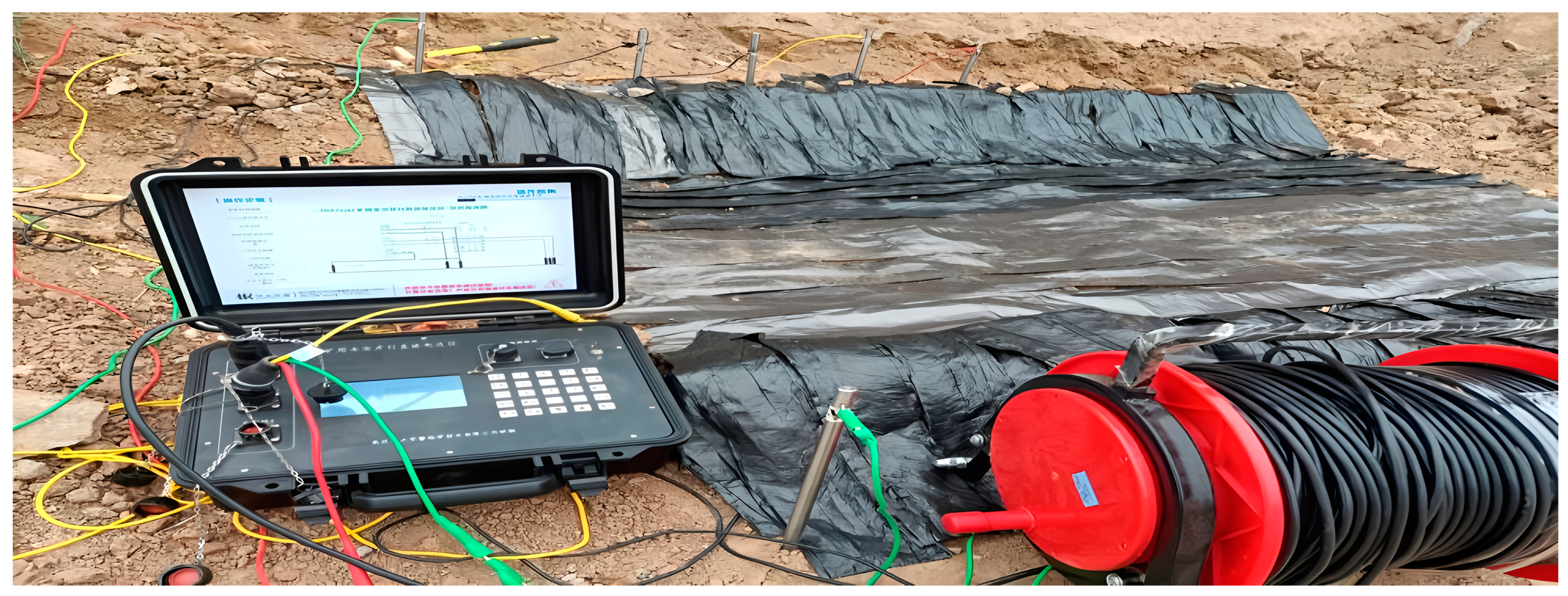
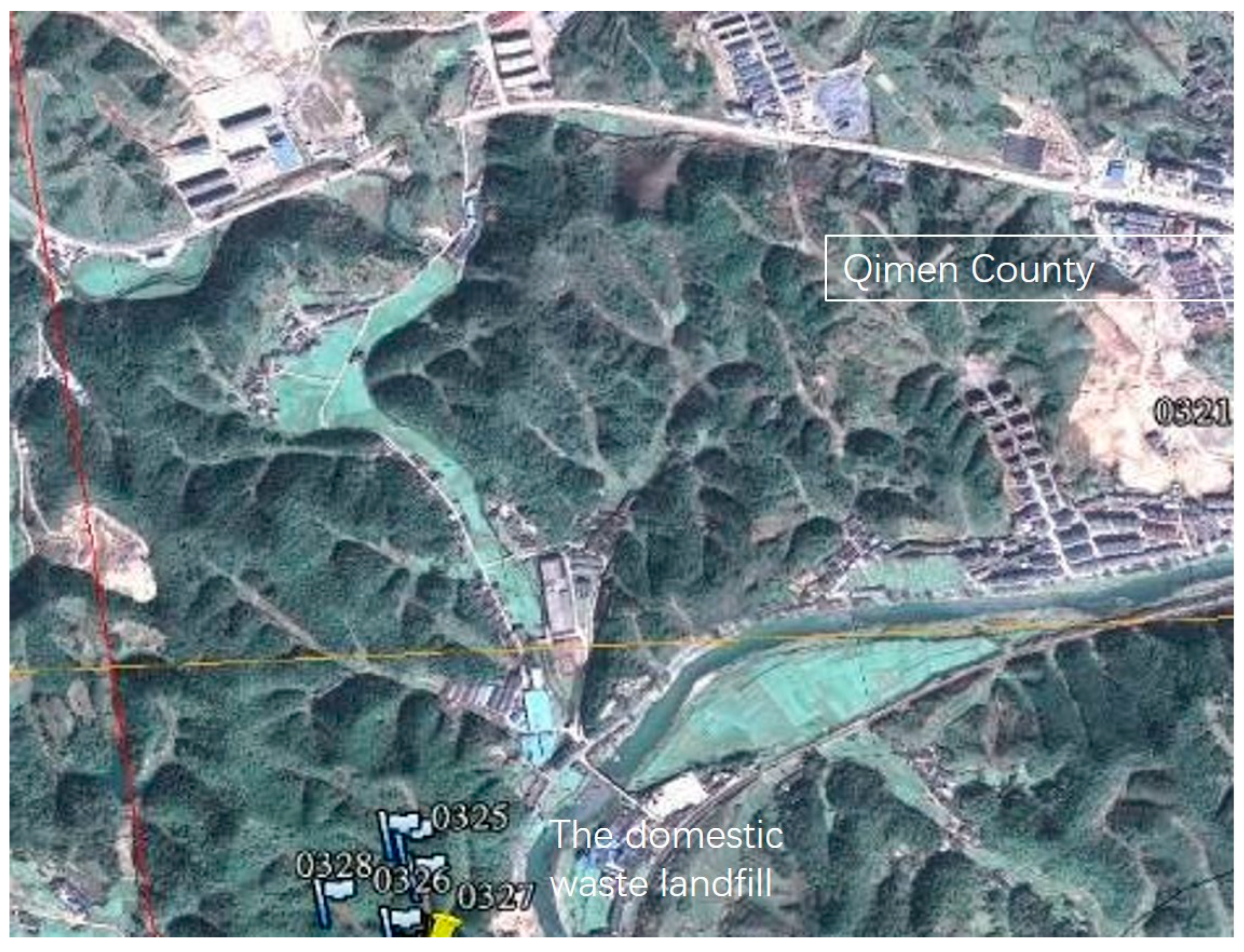
6.2.3. Real-World Scenario Experiments

The domestic waste landfill in Qimen County, Anhui Province, was completed in April 2010, with a capacity of 1.4 million cubic meters. Utilizing natural gullies, it has a valley-type layout. The anti-seepage layer at the bottom of the landfill covers an area of approximately 6000 square meters and consists of geotextiles, a 30 cm fine crushed-stone layer, two layers of geotextiles, an HDPE anti-seepage membrane, and a base layer. The regional schematic diagrams are shown in Figure 22 and Figure 23. The main object of this detection is the HDPE membrane at the bottom, and the detection area is Area 2 with an area of 800 square meters. The YDZ75 parallel resistivity tomography instrument, equipped with the CUGDCX-1 multi-channel electrode converter, was used for the survey. Equipment were sourced from Huarui Geosciences Technology Co., Ltd. CUG in Wuhan, China. There were originally three leakage points in the area, and the detection method successfully located all of them. The comparison between the true location and the detected location of the leakage points is shown in

Table 7. Comparison of true location and detected location of leakage points.

Leakage Point Number	Actual the Leakage Point	Estimate the Leakage Point	Deviation d/(cm)
1	N 29°50.555′ E 117°41.585′ H131 m	N 29°50.554946′ E 117°41.584938′ H131 m	10
2	N 29°50.519′ E 117°41.642′ H126 m	N 29°50.51894717′ E 117°41.64193907′ H126 m	9.8
3	N 29°50.512′ E 117°41.644′ H126 m	N 29°50.51204474′ E 117°41.64405161′ H126 m	8.3

.

For the latitude direction, the formula for converting the dimension difference $\Delta \phi$ to the actual distance $d_{\phi }$ is as follows:

$$d_{\phi }=\Delta \phi \times 111\times 1000$$

(33)

For the longitude direction, the formula for longitude difference conversion $\Delta \lambda$ to the actual distance $d_{\lambda }$ is as follows:

$$d_{\lambda }=\Delta \lambda \times 111\times \cos \phi \times 1000$$

(34)

The formula for the actual error d is as follows:

$$d=\sqrt{d_{\phi }^2+d_{\lambda }^2}$$

(35)

7. Conclusions

• The resistivity tomography inversion model based on the external-electrode power supply method does not require pre-burying sensors or embedded systems. It is applicable to old landfills without pre-existing monitoring facilities, thus overcoming the limitations of traditional methods that rely on pre-installed equipment. Moreover, since this method uses off-site electrodes for monitoring, compared with other methods, the monitoring devices are not corroded by leachate, which improves the sustainability of the landfill monitoring system;
• By combining the global search ability of APSO, where adaptive inertia weight and Cauchy mutation are used to avoid local optima, with the local fine-tuning optimization of the GN method, in which the conjugate gradient method is used to accelerate convergence, the inversion accuracy can be improved. Compared with single-algorithm methods, the hybrid algorithm significantly enhances the boundary recognition clarity in the low-resistivity anomaly region and reduces the reliance on the initial model;
• The maximum deviation between the inferred leakage location and the actual location is 10.1 cm, and the minimum is 6.4 cm, which meets the engineering requirements. The resistivity inversion area can effectively identify both simple point-source leakage points and line-source leakage points;
• This experiment can identify the shapes of simple point-source and line-source leakage points. However, it cannot recognize the shape of irregular leakage points. In the future, the algorithm should be further optimized to enhance the universality and accuracy of the method. Moreover, this method could potentially be developed into an automated monitoring system in the future, which would further improve the management efficiency of landfills and the environmental monitoring capabilities.

References

1. Daso, A.P.; Nevondo, V.; Okonkwo, O.J.; Malehase, T. Leachate Seepage from Landfill: A Source of Groundwater Mercury Contamination in South Africa. Water SA 2019, 45, 225–231. [Google Scholar] [CrossRef]
2. Hassan, A.; Pariatamby, A.; Ossai, I.C.; Ahmed, A.; Muda, M.A.; Wen, T.Z.; Hamid, F.S. Bioaugmentation-Assisted Bioremediation and Kinetics Modelling of Heavy Metal-Polluted Landfill Soil. Int. J. Environ. Sci. Technol. 2022, 19, 6729–6754. [Google Scholar] [CrossRef]
3. Al-Yaqout, A.; Hamoda, M.F. Long-Term Temporal Variations in Characteristics of Leachates from a Closed Landfill in an Arid Region. Water Air Soil Pollut. 2020, 231, 319. [Google Scholar] [CrossRef]
4. Ayolabi, E.A.; Oluwatosin, L.B.; Ifekwuna, C.D. Integrated Geophysical and Physicochemical Assessment of Olushosun Sanitary Landfill Site, Southwest Nigeria. Arab. J. Geosci. 2015, 8, 4101–4115. [Google Scholar] [CrossRef]
5. Ben Othmen, A.; Bouassida, M. Detecting Defects in Geomembranes of Landfill Liner Systems: Durable Electrical Method. Int. J. Geotech. Eng. 2013, 7, 130–135. [Google Scholar] [CrossRef]
6. Vrijheid, M. Health Effects of Residence near Hazardous Waste Landfill Sites: A Review of Epidemiologic Literature. Environ. Health Perspect. 2000, 108, 101–112. [Google Scholar] [CrossRef] [PubMed]
7. Pandey, L.M.S.; Shukla, S.K. An Insight into Waste Management in Australia with a Focus on Landfill Technology and Liner Leak Detection. J. Clean. Prod. 2019, 225, 1147–1154. [Google Scholar] [CrossRef]
8. Nai, C.; Wang, Y.W.; Wang, Q.; Dong, L. Setup of High Voltage Direct Circuit Equivalent Circuit Model in Leakage Detection of Landfill. Environ. Sci. 2005, 26, 200–203. [Google Scholar] [CrossRef]
9. Yang, P.; Jiang, T.; Li, Z.-C.; Yang, K.; Zhang, S.-H. Research Progress on Methods of Landfill Seepage Detection and Seepage Control. Environ. Eng. 2017, 35, 129–132+142. [Google Scholar] [CrossRef]
10. Parra, J.O. Electrical Response of a Leak in a Geomembrane Liner. Geophysics 1988, 53, 1445–1452. [Google Scholar] [CrossRef]
11. Chen, Y.; Yang, J.; Sun, H.; Wang, C. Research on Leakage Positioning of Solid Waste Landfill Based on Transmission Line Method. Environ. Eng. 2018, 36, 128–133+154. [Google Scholar] [CrossRef]
12. Chen, Y.; Huang, X.; Sun, H.; Zhang, W. Impermeable Layer Leakage Detection using a Transmission Line Model. In Proceedings of the 2019 4th International Conference on Mechanical, Control and Computer Engineering (ICMCCE), Hohhot, China, 24–26 October 2019; pp. 780–7803. [Google Scholar] [CrossRef]
13. Chen, Y.; Wang, Z.; Nai, C.; Dong, L. Computer Simulation of Transmission Line Model for Landfill Leakage Location. Adv. Mater. Res. 2012, 466–467, 416–420. [Google Scholar] [CrossRef]
14. Xie, X.; Xia, X.; Gao, Z. Optimal Arrangement of Structural Sensors in Landfill Based on Stress Wave Detection Technology. J. Sens. 2022, 2022, 7797856. [Google Scholar] [CrossRef]
15. Konstantaki, L.A.; Ghose, R.; Draganov, D.; Heimovaara, T. Wet and Gassy Zones in a Municipal Landfill from P- and S-Wave Velocity Fields. Geophysics 2016, 81, EN75–EN86. [Google Scholar] [CrossRef]
16. Chen, Y.; Sun, H.; Zhang, W.; Huang, X. Using Stress Wave Technology for Leakage Detection in a Landfill Impervious Layer. Environ. Sci. Pollut. Res. 2019, 26, 32050–32064. [Google Scholar] [CrossRef]
17. Sweeney, J.J. Comparison of electrical resistivity methods for investigation of ground water conditions at a landfill site. Groundw. Monit. Remediat. 1984, 4, 52–59. [Google Scholar] [CrossRef]
18. Binley, A.; Daily, W.; Ramirez, A. Detecting leaks from environmental barriers using electrical current imaging. J. Environ. Eng. Geophys. 1997, 2, 11–19. [Google Scholar] [CrossRef]
19. Aristodemou, E.; Thomas-Betts, A. DC resistivity and induced polarization investigations at a waste disposal site and its environments. J. Appl. Geophys. 2000, 44, 275–302. [Google Scholar] [CrossRef]
20. Binley, A.; Daily, W. The performance of electrical methods for assessing the integrity of geomembrane liners in landfill caps and waste storage ponds. Environ. Eng. Geophys. 2003, 8, 227–237. [Google Scholar] [CrossRef]
21. Resurs, R. Resistivity-IP mapping for landfill applications. First Break 2010, 28, 40–45. [Google Scholar] [CrossRef]
22. Abdulrahman, A.; Nawawi, M.; Saad, R.; Abu-Rizaiza, A.S.; Yusoff, M.S.; Khalil, A.E.; Ishola, K.S. Characterization of active and closed landfill sites using 2D resistivity/IP imaging: Case studies in Penang, Malaysia. Environ. Earth Sci. 2016, 75, 347. [Google Scholar] [CrossRef]
23. Akintorinwa, O.J.; Okoro, O.V. Combined electrical resistivity method and multi-criteria GIS-based modeling for landfill site selection in the Southwestern Nigeria. Environ. Earth Sci. 2019, 78, 162. [Google Scholar] [CrossRef]
24. Archie, G.E. The electrical resistivity log as an aid in determining some reservoir characteristics. Trans. AIME 1942, 146, 54–62. [Google Scholar] [CrossRef]
25. Liu, Y.; Cai, H.; Hu, X.; Peng, R. 3D Forward Modeling and Analysis for Loop-Source Transient Electromagnetic Data Based on Finite-Volume Method in an Arbitrarily Anisotropy Earth. In Proceedings of the International Workshop on Gravity, Electrical & Magnetic Methods and Their Applications, Xi’an, China, 19–22 May 2019. [Google Scholar] [CrossRef]
26. Sasaki, Y. 3-D resistivity inversion using the finite-element method. Geophysics 1994, 59, 1839–1848. [Google Scholar] [CrossRef]
27. Loke, M.H.; Dahlin, T. A Comparison of the Gauss–Newton and Quasi-Newton Methods in Resistivity Imaging Inversion. J. Appl. Geophys. 2002, 49, 149–162. [Google Scholar] [CrossRef]
28. Guo, L.; Wu, S.; Yang, B.; Dai, G. Three-Dimensional Direct Current Resistivity Finite Element Method Forward Modelling Based on Jacobi Preconditioned Conjugate Gradient Algorithm. J. Nanoelectron. Optoelectron. 2023, 18, 176–183. [Google Scholar] [CrossRef]
29. Loke, M.H.; Barker, R.D. Practical Techniques for 3D Resistivity Surveys and Data Inversion. Geophys. Prospect. 1996, 44, 499–523. [Google Scholar] [CrossRef]
30. Qin, G.; Xiao, X. Three-dimensional NLCG inversion by DC method based on unstructured grid. Chin. J. Eng. Geophys. 2024, 21, 473–483. [Google Scholar] [CrossRef]
31. Liu, B.; Li, S.C.; Nie, L.C.; Wang, J.; Zhang, Q.S. 3D Resistivity Inversion Using an Improved Genetic Algorithm Based on Control Method of Mutation Direction. J. Appl. Geophys. 2012, 87, 1–8. [Google Scholar] [CrossRef]
32. Pidlisecky, A.; Haber, E.; Knight, R. RESINVM3D: A 3D Resistivity Inversion Package. Geophysics 2007, 72, H1–H10. [Google Scholar] [CrossRef]
33. Zhang, J.; Mackie, R.L.; Madden, T.R. 3-D Resistivity Forward Modeling and Inversion Using Conjugate Gradients. In SEG Technical Program Expanded Abstracts; Society of Exploration Geophysicists: Tulsa, OK, USA, 1994. [Google Scholar] [CrossRef]
34. Zohdy, A.A.R. A New Method for the Automatic Interpretation of Schlumberger and Wenner Sounding Curves. Geophysics 1989, 54, 245–253. [Google Scholar] [CrossRef]
35. Liu, B.; Li, S.; Li, S.; Nie, L.; Zhong, S.; Li, L.; Song, J.; Liu, Z. 3D electrical resistivity inversion with least-squares method based on inequality constraint and its computation efficiency optimization. Chin. J. Geophys. 2012, 55, 260–268. [Google Scholar] [CrossRef]
36. Liu, B.; Liu, Z.Y.; Song, J.; Nie, L.C.; Wang, C.W.; Chen, L. Joint inversion method of 3D electrical resistivity detection based on inequality constraints. Chin. J. Geophys. 2017, 60, 820–832. [Google Scholar] [CrossRef]
37. Zha, Y.; Yang, J.; Zeng, J.; Tso, C.H.; Zeng, W.; Shi, L. Review of Numerical Solution of Richardson–Richards Equation for Variably Saturated Flow in Soils. WIREs Water 2019, 6, e1364. [Google Scholar] [CrossRef]
38. Faraj, I.S.; Abid, M.B. Water Movement through Soil under Drip Irrigation Using Different Hydraulic Soil Models. J. Eng. 2020, 26, 43–61. [Google Scholar] [CrossRef]
39. Jafari, Z.; Matinkhah, S.; Mosaddeghi, M.R. Wetting Patterns in a Subsurface Irrigation System by Using Reservoirs of Different Permeabilities: Experimental and HYDRUS-2D/3D Modeling. Water Resour. Manag. 2022, 36, 5335–5352. [Google Scholar] [CrossRef]
40. Cheng, H.; Liu, P.K.; Wang, Y.L.; Nai, C.X. Determination of dipole spacing in electrical landfill leakage detection. Adv. Mater. Res. 2011, 171, 171–174. [Google Scholar] [CrossRef]
41. Guan, S.P.; Wang, Y.W.; Nai, C.X.; Dong, L. Comparison of Two Electrode Arrays for Liner Leakage Location at Landfills. In Proceedings of the 2009 4th IEEE Conference on Industrial Electronics and Applications, Xi’an, China, 25–27 May 2009. [Google Scholar] [CrossRef]
Figure 1. Schematic diagram of detection principle.
Sustainability 17 04044 g001
Figure 2. Distribution of current density on both sides of the HDPE membrane.
Sustainability 17 04044 g002
Figure 3. Potential distribution model beneath the membrane.
Sustainability 17 04044 g003
Figure 4. Schematic diagram of the detection model.
Sustainability 17 04044 g004
Figure 5. Flowchart of the APSO combined with the G-N method for inversion.
Sustainability 17 04044 g005
Figure 6. Three-dimensional space model.
Sustainability 17 04044 g006
Figure 7. Grid division and electrode configuration model. (a) Section XOY, (b) section XOZ.
Sustainability 17 04044 g007
Figure 8. Imaging results using the Gauss–Newton method. (a) y = 3.5 m; (b) z = −2.5 m.
Sustainability 17 04044 g008
Figure 9. Imaging results of the adaptive particle swarm algorithm. (a) y = 3.5 m, (b) z = −2.5 m.
Sustainability 17 04044 g009
Figure 10. Imaging results of the adaptive particle swarm algorithm combined with the Gauss–Newton method. (a) y = 3.5 m; (b) z = −2.5 m.
Sustainability 17 04044 g010
Figure 11. RMS variation during iterative inversion of the combined algorithm.
Sustainability 17 04044 g011
Figure 12. Simulation model. (a) Circular leak model; (b) linear leak model.
Sustainability 17 04044 g012
Figure 13. Leachate movement pattern. (a) Point-source leakage XOZ section, (b) line-source leakage XOZ section, (c) point-source leakage XOY section, (d) line-source leakage XOY section.
Sustainability 17 04044 g013
Figure 14. Schematic diagram of the experiment.
Sustainability 17 04044 g014
Figure 15. Test scenario diagram.
Sustainability 17 04044 g015
Figure 16. Three-dimensional resistivity tomography map. (a) No leakage chromatogram, (b) Gauss–Newton method, (c) adaptive particle swarm optimization, and (d) joint algorithm.
Sustainability 17 04044 g016
Figure 17. Three-dimensional tomographic cross-sectional view. (a) YOZ section; (b) XOZ section.
Sustainability 17 04044 g017
Figure 18. Sectional view of XOY. (a) Adaptive particle swarm optimization, (b) Gauss–Newton Method, and (c) joint algorithm.
Sustainability 17 04044 g018
Figure 19. Point-source inversion diagram. (a) z = −0.5 m, (b) y = 1 m.
Sustainability 17 04044 g019
Figure 20. Line-source leakage point inversion diagram. (a) z = −0.5 m, (b) y = 1 m.
Sustainability 17 04044 g020
Figure 21. Point-source inversion diagram with half original time. (a) z = −0.5 m, (b) y = 1 m.
Sustainability 17 04044 g021
Figure 22. Location map of Qimen domestic waste landfill.
Sustainability 17 04044 g022
Figure 23. Schematic diagram of landfill detection area division.
Sustainability 17 04044 g023