Abstract
While the speed of the transition to battery electric vehicles (BEVs) depends on real-world driving behaviors and socioeconomic conditions, relevant predictions are often not based on real trip data. This study analyzes over 200,000 private car trips, tracked via onboard telematics across Italy, in order to assess the feasibility of replacing internal combustion engine vehicles (ICEVs) with BEVs. Given that drivers are resistant to changing their habits, we introduce the E-Private Mobility Index, which quantifies the percentage of traditional cars at present that are functionally compatible with a medium BEV, assuming home charging. Nationwide, this index reaches 30%, but only 15% of car owners would also see financial benefits. By quantifying both the potential to replace traditional cars with electric ones and the associated economic impacts, our analysis supports sustainable mobility by offering insights into the rate of penetration of sustainable and green mobility, in line with the objectives of the European Green Deal. With its unprecedented statistical significance, the study not only provides a data-driven upper threshold of BEV penetration but also offers a flexible framework for shaping future policies, allowing the adaptation of parameters and assumptions to guide a scalable transition to electric private mobility.
1. Introduction
Battery electric vehicles (BEVs) play an essential role in the achievement of sustainable transportation. However, the penetration rate of private fully electric cars in the Western world is significantly lower than the expectations from about ten years ago. Nevertheless, the European Union has recently confirmed the targets of the European Green Deal [1], which requires a 90% reduction in greenhouse gas emissions by 2050; for the nearest target in particular, the EU has reaffirmed the complete transition to electric vehicles by 2035 [2], as have previous European and international studies and agreements [3,4,5].
Before delving into the problem statement, it is important to highlight the key emerging issues related to enabling the diffusion of BEVs and accelerating their adoption. The challenges span technological, economic, infrastructural, and behavioral aspects. The most impactful challenges concern consumer perception and behavioral shifts, government policies and incentives together with stringent emission regulations and urban access regulations, low-cost charging infrastructure expansion and accessibility, and battery supply chains that must be affordable from both economic and environmental perspectives. In our research, our primary goal was to demonstrate, through a model driven by today’s real private mobility data, how these challenges that we just outlined are indeed the key enablers of an increasingly electric and sustainable vehicle fleet. In the context of understanding this mobility transition, experts in different fields, from sociology to transportation planning and big data analysis, aim to explain the current context in order to more realistically predict the extent to which private transportation and people’s habits are compatible with fully battery-powered cars and, consequently, what growth rate for these vehicles we can expect in the near future. These issues have been extensively discussed in the literature. In [6], the authors provided a comprehensive bibliographic review of the mathematical modeling techniques used to represent the BEV adoption process. In [7,8], studies were presented on the transition to BEVs in US cities, while [9] provided a wider analysis on the energy transition in the US, also focusing on electric mobility. In [10], the researchers highlighted the economic effects of the political decisions to ban fossil fuel vehicles, and the authors of [11] described the climate change mitigation potential of a significant transition to BEVs. The authors of [12] gave a perspective on social equity when considering a transition to electric mobility while taking into account the different economic strata in the population. On the same topic, the authors of [13] focused on the importance of the social and economic sustainability of the energy transition in mobility. In [14], the costs of a rapid transition to electric mobility were quantified, while the authors of [15] evaluated the impact of the transition to BEVs in India and the effects on the involved stakeholders. The authors of [16] addressed the effect of electrification in China. As the BEV adoption process has somewhat slowed down due to high purchase prices and concerns about limited battery range and inadequate public charging infrastructure, in [17], the authors used a massive real-world dataset containing anonymized global positioning system (GPS) traces from a fleet of private vehicles to quantitatively evaluate whether range anxiety (fear of being stranded due to the limited range of electric vehicles) is a rational concern. The results presented in [17] revealed the potential of BEVs, which could satisfy the range demands placed on a significant number of existing fuel-powered vehicles without altering the owners’ routines. The research in [17] also quantitatively evaluated the effects of increasing the dissemination of charging facilities on vehicles’ operational suitability for replacement by BEVs. Additionally, the first pilot study in Italy in this field was carried out in [18].
In this work, we are specifically interested in the transition from private internal combustion engine vehicles (ICEVs) to BEVs. The major trend in mobility will most likely be fully electric cars, followed by autonomous and shared vehicles. The various long-established forms of shared mobility support, apart from cost efficiencies and sustainability, include optimizing cities’ parking spaces and infrastructure use [19]. The authors of [20] proposed an overview of shared electric mobility and highlighted advantages and beneficial effects from both economic and environmental perspectives, demonstrating the significance of the transition for sustainability. The in-depth analysis in [21] revealed that shared electric mobility is not valuable if it does not bring an economic advantage for the user [22]. This also represents the foundation of our work, as we aim to demonstrate—while still considering the private ownership of cars—the conditions under which fully electric mobility is functionally and economically advantageous. This happens if the driving habits of car owners are characterized by high annual mileage and low distances (and this is exactly what shared mobility enables). Moreover, in a recent cutting-edge study (accepted but not yet published), we show, through simulation with a simplified model, that only with the transition from traditional free-floating car sharing to an autonomous urban on-demand shared mobility service will it be possible to enable high mileage for each vehicle and, thus, fully utilize the batteries’ end-of-life capacity, which is approximately 2000 charge cycles. In fact, in [23], the authors illustrated the main emerging technologies that would accelerate the adoption of electric vehicles, namely, shared mobility and vehicle automation. Although we consider only private mobility in this study, the endpoint condition of electric fleet benefits would be achieved by following these promising trends. For this reason, as well as to provide a clear and understandable focus for this article, hybrid cars are not considered. We propose an in-depth analysis based on a large set of existing telematic private mobility data geographically spread over different Italian regions, in order to reach statistically solid conclusions about the feasibility of transitioning to fully electric motor transport. The analysis is naturally supported by somewhat necessarily restrictive assumptions that, in our opinion, take into account the most impactful factors—at least, in an initial analysis—regarding compatibility with the use of a fully electric private vehicle: battery range limitations, charging needs, and economic factors. Furthermore, by comparing significantly different provinces, we show how factors such as industrial development, urban planning, and socioeconomic conditions affect the scale and rapidity of the transition.
This work joins the very few studies on private mobility electrification in the literature—see, for example, refs. [24,25]—which derive results and insights from continuous tracking of numerous vehicles over time and space across an extended period, rather than relying on surveys, questionnaires, and small datasets related to a limited class of vehicles or traffic models. The primary outcome of this work is the evaluation, through the ad hoc-coined E-Private Mobility Index, of a feasible percentage of current private vehicles in Italy that are used with a travel distances behavior compatible with a medium-size BEV autonomy, under some simplifying (but, in our opinion, very reasonable) assumptions. We evaluate the functional feasibility of the driven distances for each trip of each vehicle with the average autonomy capacity of the reference BEV battery (assumed to be equal to 300 km with a very cautious and conservative mindset, but this is cost-effective) under the hypotheses that domestic recharging is possible and that no one should need to recharge at a high cost outside their home, where, moreover, the infrastructure would not yet be widespread.
The results highlight that the possibility of electrification (replacing ICEVs with BEVs) is not uniform across the national territory but varies depending on each province’s geographical extension, industrial and service density, and distinctive population habits. Second, once the functional feasibility is assessed, it is cross-referenced with a thorough economic analysis of the purchase, operation, and maintenance of BEVs while remaining easy to understand and interpret. The ultimate outcome of this part of the work highlights how often, in terms of the number of functionally feasible drivers, a reasonable breakeven time (years necessary to amortize the excess expenses for a BEV compared to an ICEV) occurs. Factors such as purchase price, presence/absence of public incentives, maintenance and insurance costs, operating expenses, charging costs, and annual mileage heavily affect the economic feasibility of the investment. In this study, we do not consider the psychological attitude and preferences of drivers, which is also because, as mentioned, this is typically the subject of studies that are necessarily based on surveys or questionnaires; see, for example, [26,27]. The focus of this work is on demonstrating the feasibility of an economic and driving-style-compatible transition from ICEVs to BEVs. This allows us to exclude the analysis of BEV repurchase likelihood from the study, as we exclusively consider first-time buyers. Considering the impact of “brand perception” on a candidate electric vehicle owner (which we recognize as a relevant aspect in the decision of a BEV purchase), in this study, we do not specify any brands but consider an economical reference car with low in-line market prices. The considered perspective covers the economic advantage of considering a BEV purchase given the driving pattern of a current ICEV owner. The structure of the remainder of this article is as follows. In Section 2, the available original anonymized datasets, their preprocessing, and the data-cleaning phases are described in detail. In Section 3, domestic or close-to-home charging clusters are computed from trips’ spatiotemporal coordinates. In Section 4, the functional feasibility of the E-Private Mobility Index is introduced, and data are mined to derive it for each region and nationwide. In Section 5, the economic feasibility of a BEV purchase is described in detail and combined with a functional assessment. Section 6 summarizes the key findings of the study and concludes the article with potential areas for further exploration.
2. Data Description and Preprocessing
In this section, we describe the data made available by UnipolTech, the technology company of the primary Italian insurance group Unipol Group, and how they were processed. The data are completely anonymized; no information on vehicle owners’ personal data is available, following current Italian privacy regulations and laws. The data collection covered the full year of 2022 (we have verified that in Italy, by January, private traffic had already returned to pre-COVID levels), and approximately 360 million trips were tracked by black boxes that were firmly installed onboard and stored for over 226,000 vehicles, which were divided as follows: for the Bari province, 81,460 vehicles (60% of the cars in Bari were equipped with telematic boxes) with 140 million trips; for the Rome province, 91,927 vehicles ( of the black-box-enabled cars) for a total of 150 million trips; for the Brescia province, 53,412 vehicles ( of the black-box-enabled cars in this province) for a total of 70 million trips. As can easily be understood, continuous tracking of all of these vehicles for a year provided an enormous amount of information about their movements and their drivers’ habits.
The starting datasets consist of GPS measurements, sampled at 1 Hz. Each GPS sample, denoted as an event, is sent to a remote server. From the raw measurements, for each vehicle, we further carried out non-trivial processing that took into account both space and time to obtain trips as primary elements (sequences of start–active–stop) for each vehicle. Since data are available in massive quantities there, this study is focused on the Italian provinces of Brescia, Rome, and Bari as representatives of northern Italy, characterized by significant industrial development and placed within a flat area, the Padana plain, with extensive economic activities and development; of central Italy, with a very large road network that mandates high daily distances for commuters; and of southern Italy, featuring a compact city center but an evolved industrial network. Reasonably, the results for these Italian regions could, in some cases, be methodologically generalized to similar areas across the European continent. However, to obtain precise feasibility indicators, a significant dataset from the province of interest would be necessary.
In greater detail, the event data information is organized as follows. For each recorded event, the vehicle ID is registered. This ensures the possibility of identifying each vehicle independently. Each event has its own event type, which is representative of the vehicle engine condition. The type is saved as an integer variable 0, 1, or 2, representing, respectively, the following engine states: start, active, stop. Therefore, a typical sequence of event types will be the following: . This covers the engine’s activation, the sequence of active engine events, and, ultimately, the stopping of the engine. The availability of this unique code is fundamental for each trip’s reconstruction. Temporal information is provided as GPS event timestamps and the time gap between two consecutive events. Latitude and longitude coordinates are given together with the distance traveled from the last event registered. The vehicle speed at the event time is saved. Additional information (that is not used in this study), such as vehicle heading and speed, GPS signal quality, and road type, are available as well and might be used in different analyses. It is important to clarify here that all of the datasets provided to us originally had good or excellent GPS quality.
Given each vehicle’s event information headers, which are summarized in Table 1, the first step involves the aggregation of this event-based information into a complete trip-based set for each vehicle in the dataset. To achieve this goal, sequences of start–active–stop events are identified, and the duration of the stop following a trip’s end is attached. In this way, for each car, every trip taken in the observation period is reconstructed, and its information structure is organized according to the fields specified in Table 2.

Table 1.
Event data fields.
Table 2.
Trip data fields.
Due to errors and inaccuracies in the original data acquisition, preprocessing of corrupt and misleading trips is necessary. The objective of this cleaning procedure was to identify trips of vehicles affected by inconsistencies in the data measurement phase performed by the black boxes and to correct these errors when possible or otherwise remove them from the dataset. Before introducing the filtering policies, we need to introduce the haversine formula. It determines the great-circle distance between two points on a sphere given their longitudes and latitudes and the radius of the sphere. It has applications in air and marine navigation, and, in our case, we use it to accurately measure the trip length given the trip start and destination coordinates. The haversine formula (see [28]) is defined as follows:
where the variables are defined as follows:
- d is the distance between two points on the surface of a sphere with radius r;
- and are the latitudes of the two points in radians;
- and are the longitudes of the two points in radians;
- is the haversine function.
Thus, based on the formula outlined above, the distance between the origin and destination of each available trip was calculated, along with the total length.
We acknowledge that the haversine distance is a proxy of the actual road distance. However, in this study, we apply the haversine distance, as it is widely recognized in the literature ([29,30]) as a reasonable first approximation given its computational efficiency, especially in large-scale simulations. Future work will include the implementation of correction factors derived from real-world data to refine the haversine result.
With this information, cleaning to remove defective trips could be executed as follows:
- Zero-distance trips: All trips resulting in a distance of 0 m traveled were removed. They are associated with start–active–stop engine sequences where the GPS coordinates (latitude and longitude) do not show a meaningful variation.
- Excessively short or long trips: Extremely short (less than 3 min) or extremely long (more than 16 h) trips have no meaning and are probably outliers. They are not representative of standard driving conditions. The trip duration and the subsequent stop duration were defined so that trips with a total durationcould be eliminated.
- Excessively slow or fast trips: All trips with an extremely low or extremely high average speed, which is not representative of normal driving conditions, were filtered out. These instances might have different causes, such as traffic jams, queues at extremely low speeds, dangerous high-speed driving, and, of course, black box measurement errors. We removed trips where the average speed v was
- Unreliable vehicles: Given the previous filters on trips, we further applied a restriction on vehicles (not trips in this case) where a non-negligible portion of the total number of trips was removed by the previous skim. Hence, we removed vehicles for which least trips fell under the previously mentioned data-cleaning cases.
Table 3 summarizes the number of cars (with their black boxes) originally provided, the number of “clean” cars after the preprocessing procedure, and the total number of trips in the considered provinces.
Table 3.
Clean trip dataset characteristics—observation period: 1 December 2021 to 30 Novermber 2022.
3. Proximity Charging Cluster Identification
After the conversion of the events into trips and the dataset cleaning process, we needed to geographically identify the “homes” of the cars, since the data were anonymized and no information on the geographical residence was available. This meant locating the candidate domestic charging points where, based on our strong yet reasonable assumptions, a potential electric car’s battery could recharge. These “homes” are naturally associated with the recurrent night parking clusters for each vehicle. We made the further assumption that public charging would also be possible, as long as the charging station (to be clear, those placed along sidewalks in cities) is close to a candidate “home”. If the charging station was on the street and shared, we assumed that there would always be one available due to the persistent increase in proximity infrastructure.
As described in detail below, the algorithm for defining cars’ “homes” identified clusters with repeated and sufficiently long stops during the night. Multiple clear, regular nighttime stopping points could be extracted, and based on a logic of priority, the three main “homes” from these points were assigned to each car.
For each car, the accurate recognition of the home location was performed by executing the Density-Based Spatial Clustering of Applications with Noise (DBSCAN) algorithm (see [31]) based on the spatial density of the destination points. This allowed us to identify areas where a vehicle made frequent stops. DBSCAN requires the following two input parameters:
- : the maximum distance such that two destination points are considered close;
- : the minimum number of destination points required to form a cluster.
For each car with its trips, the algorithm starts from a random destination point, computes its -neighborhood, and, if it contains enough other destinations, a new cluster is defined. If not, the data point is labeled as noise and may later be found in a different cluster. The process continues until all input destination points are processed.
In our case, the values chosen for the two hyperparameters were selected following a sensitivity analysis and set to m and , meaning that we require that at least stops have been made within a distance of . The additional and key concept for this analysis is that destination stops must extend across the date change (i.e., occur overnight, when it is reasonable to assume that the car is parked at home or nearby) and must also be sufficiently long. The, to detect “homes” or night clusters properly, the following considerations were taken into account:
- The date must change during the stop; in this way, we can capture all of the stops starting before midnight (of each day) and ending after it.
- The stop duration is at least 8 h; with this second constraint, we can capture all stops starting before midnight and ending after it, with a duration of at least 8 h, which is compatible with a night’s rest.
With these two filters, we have the confidence of having selected only stops that represent nighttime behavior.
This allows us to identify “home” clusters that can be considered places for charging a BEV.
Figure 1 shows the identified “homes” or night clusters of the cars registered in Bari and its province. For the same car, more than one cluster might be identified. Each cluster is sorted according to a ranking depending on the absolute frequency of the stops in that cluster with respect to the total number of stops. The most important clusters (darker in Figure 1) have a higher absolute frequency of night stops, whereas the less important (brighter in Figure 1) have a lower quantity of clustered night destination points.
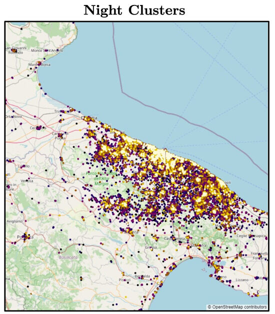
Figure 1.
“Homes” or night clusters of the registered vehicles in the Bari province. For the same car, many clusters might exist. A darker color indicates more important clusters, where the vehicles often stop during the night. A brighter color indicates clusters with lower relative frequency, meaning that the car stops in the identified cluster for a reduced number of nights.
Figure 2 shows, for each province, the percentage of vehicles for which zero, one, or more night clusters were identified. For the majority of the cars, night clusters were successfully detected. For spurious vehicles, clusters were not found. It depends on the additional inconsistency of the collected data and DBSCAN settings. Different configuration settings might slightly change the percentages shown.
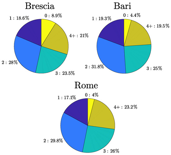
Figure 2.
Percentages of vehicles with 0, 1, 2, 3, and “homes” or night clusters in Brescia, Bari, and Rome, respectively.
The present research focuses on the detection of night clusters given the working hypotheses of charging at “homes” (or in its proximity) in one of the identified clusters (it should be noted that charging can be performed during different stops, as well as during the day and in any of the identified “homes”). The inclusion of day clusters (workplace for example) is outside the scope of this study but might be considered in future development if the possibility of charging at the workplace can be considered feasible in practice.
To avoid excessive complexity in the analysis, we will refer only to the three main “homes” and discard any night clusters identified through spatial clustering that contain too few nighttime stops. This choice corresponds to the hypothesis of assuming that one recharges either at one’s habitual residence (“home”) or at one’s possible second or third place of accommodation.
Figure 3 shows that the majority of vehicles have a long stop frequency close to zero at the second or third “homes” and a visibly high frequency of long night stops at the main residence. The maximum frequency in the tertiary cluster is about , while in the secondary cluster, it is . The majority of vehicles have a frequency of around 90–100% attendance of the main cluster, that is, the main “home”.
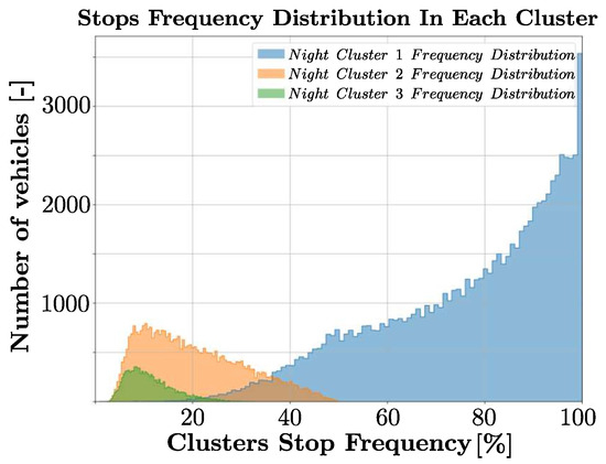
Figure 3.
Absolute frequency distribution of vehicles’ stops in their first, second, and third night clusters.
After correctly recognizing the candidate charging locations, in our hypotheses, we identified users who traveled a distance shorter than that guaranteed by the actual battery capacity limit between two charging-compatible stops in either one of the discerned clusters. This is the content illustrated in the next section.
4. E-Private Mobility Index
In this section, we introduce the E-Private Mobility Index, which represents the percentage of actual ICEVs (whose travel behavior is represented in the telematic datasets) that could effectively be replaced by BEVs. This indicator depicts the compatibility of the distances traveled by each car between two consecutive stops at private charging sites with the maximum distance allowed by the battery capacity. This index considers the length of the vehicle’s trips and assumes the existence of low-cost charging points at or near the vehicle owners’ homes. Widespread fast-charging infrastructure is still very much in its development phase in Italy and significantly more expensive than home or public proximity slow-charging stations. Hence, the choice of assuming that charging is performed only at a domestic parking space or at a convenient proximity charging station is justified. To be cautious, we assume the availability of recharging power to be equal to 7.4 kW [32] at each mentioned useful recharging location.
The economic feasibility of the amortization of excess expenses linked to the purchase of a BEV (compared with an ICEV) was computed a posteriori only for cars satisfying the functionally feasible behavior-based analysis presented hereafter.
Here, we show how the vehicles ready to switch to fully electric motorization were identified. The reference range of battery autonomy is 300 km. This range is currently achievable (and conservative) for the majority of private BEVs on the market ([33,34]). The working hypothesis is that each vehicle can recharge in one of its clusters, , and it is considered suitable for replacement with a BEV if the distance driven within each trip never exceeds (or is, at most, times) the battery autonomy range. The algorithm specifically developed to extract cars based on the aforementioned conditions is structured through the following steps:
- The stops compatible with recharging are identified, and this compatibility assumes that the following conditions are satisfied:
- Recharging can be carried out in one of the “homes”.
- The duration of the stop for it to be compatible with a top-up must be at least 5 h. Of course, this time interval can be shortened as desired.
- The stop must be located within 250 m from the center of the respective “homes” cluster. This quantity refers to m, the parameter employed to define clusters.
- All trips between two stops compatible with recharging are aggregated because, between these stops, it is supposed (in our model) that recharging the battery is not possible.
- For each aggregate of trips, the total distance traveled is calculated.
- The number of times the battery range (300 km) is exceeded by each aggregate of trips is computed and stored as , that is, the “exceeding” aggregate of trips.
Figure 4 shows how the percentage of vehicles that could be immediately electrified based on their trip–stop behavior is a function of the following:
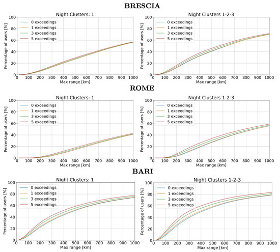
Figure 4.
Percentage of cars out of all cars in the cleaned datasets vs. BEV battery autonomy range for the range of “exceeding” trip aggregates; the value of considers just the principal “homes” (left) and all three main “homes” (right) as charging locations for the Brescia, Rome, and Bari provinces.
- Battery range: As the battery capacity increases—as does, consequently, the autonomy range—the number of private ICEVs that could safely switch to fully electric increases.
- Number of charging locations: Considering only a main ”home”, = 1, results in pinpointing fewer vehicles, as expected.
- Number of tolerated battery range violations, : As the number of “exceedings” permitted in a year increases, the number of new possible BEVs also grows.
The most restrictive situation coincides with permitting recharging only in the main residence, , and allowing no “exceeding”, .
The most permissive scenario envisages the possibility of recharging in the two, if any, alternative “homes”, , and allows a number of “exceedings” of up to .
As shown by the curves in Figure 4, it is possible to derive the minimum and maximum fractions of the given private vehicle fleet (very numerous and, hence, very statistically significant) that have a mobility pattern compatible with fully electric mobility.
In Figure 5, the E-Private Mobility Index is shown. This index is dimensionally a percentage and, as the battery capacity range varies up to 500 km and or , represents the percentage of private cars in each province that were functionally compatible with replacement by a BEV. Note that Bari has a higher index than Brescia and requires greater battery capacity than Rome. Of course, Rome’s geographical extent is much greater than that of Brescia and Bari; therefore, fewer vehicles meet the requirements of the trip aggregates not exceeding the battery range and, consequently, are feasible candidates for electrification.
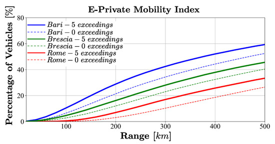
Figure 5.
E-Private Mobility Index as a function of BEV battery autonomy range for the Brescia, Rome, and Bari provinces considering the lowest extreme case of no trips exceeding the range (zero exceedings) and the highest considered case of five trips surpassing the autonomy range (five exceedings). Notably, as the battery range increases, the likelihood of trips exceeding it decreases, thereby expanding the potential compatible vehicle base. Clearly, this behavior visually allows us to understand which battery capacity would correspond to which penetration percentage of BEVs.
Overall, as the E-Private Mobility Index, we univocally take the percentage in the ordinate of the curves in Figure 5 corresponding to the abscissa of 300 km (our original autonomy range) and to (supposing that we tolerate five out-of-range trips). Moreover, up to charging locations, if they exist, are taken into account.
The E-Private Mobility Index—i.e., the fraction of all cars in the provinces’ datasets that turn out to be functionally compatible with the length of trips and duration of domestic recharging stops—is summarized in Table 4.
Table 4.
E-Private Mobility Index.
After collecting the previous results from three representative provinces in northern, southern, and central Italy, we believe that it would also be reasonable to exploit a single indicator at a national level that could include the different behaviors manifested in the territories. The nationwide evolution of car park electrification is computed simply as the average of the E-Private Mobility Index identified for the three provinces, showing that the average percentage of private car that could feasibly be replaced with fully electric cars is around of the Italian car fleet.
5. Enhancement of the Evaluation by Cross-Referencing Functional Feasibility (E-Private Mobility Index) and Economic Arguments
The goal of this section is to understand, given the previously described trip–stop–recharge feasibility analysis and the sets of vehicles compatible with an enforceable transition from internal combustion to fully electric, in the context of the illustrated hypotheses, the economic conditions of a fair breakeven situation for the purchase of a BEV compared with an equivalent ICEV.
The following economic analysis is carried out under the extreme assumption that no public incentive is available. In our scenario, it is essential to remain as independent as possible from political or governmental decisions, which are known to be highly variable and to change over time. However, these decisions can easily be incorporated into the economic model that we will present, as it is deliberately simplified and easy to modify, and, of course, any policy incentive would only reduce the time necessary to reach the breakeven point.
5.1. Annual Mileage Distribution
This section shows some considerations about the average annually driven mileage as preparation for the economic analysis.
Figure 6 shows the annual average mileage of the vehicles with and battery range “exceedings”, where recharging is considered possible in one of the three main night clusters in the three provinces. The data from Brescia and Bari clearly show cars driving a lower yearly average mileage than in Rome. This behavior depends on the greater mobility required for daily life in the Italian capital city. For each province, of course, data on vehicles with no battery range “exceedings”, , have lower annual average mileage compared with vehicles with “exceedings”. This is intuitive, as tolerating up to five recharging events away from “homes” means that vehicles are allowed to travel longer distances.
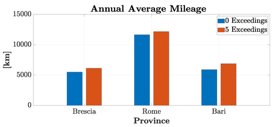
Figure 6.
Annual average mileage of cars included in the E-Private Mobility Index analysis with battery range ”exceedings” while assuming that , which indicates the possibility of charging at up to three potential “homes”.
In summary, we observe the key data-driven fact that ready-to-go BEVs would be characterized by very low annual mileage. This result suggests that, in order to achieve a sustainable electric transition, an interesting direction could be the consideration of shared mobility, in which a single electric vehicle might be used by many drivers. This would allow the exploitation of, at best, the total available mileage of the battery, avoiding discarding batteries whose useful life is still significant and reducing the economic impact and environmental pollution. At the same time, it is important to underline that only this economic advantage would be effective, which could ensure a breakeven point to be reached with cars’ original yearly mileage without the need to change one’s driving habits by forcibly boosting the driven distances. Indeed, if we consider vehicles with very high annual mileage, they are probably less likely to be feasible candidates for electrification, since they often overshoot the battery autonomy range. The “paradox” is that these very same vehicles with high annual mileage are instead potential candidates from the economic perspective as, obviously, the economic advantage increases as the traveled distance increases.
5.2. Economic Breakeven Framework
It should be kept in mind that, in this study, we deliberately assumed only at-home or near-home charging, which is slow and low-cost. Clearly, one could have assumed the use of fast- or super-fast-charging stations, but this scenario is currently beyond the scope of our analysis, primarily due to the very high costs associated with such fast-charging solutions. Thus, two different energy cost situations are regarded.
- High Energy Costs: The geopolitical situation in 2022 led to increased energy prices, particularly that of electricity, in Europe. Therefore, we consider an updated electricity/oil price, as set in that period in Italy ([35,36,37]).
- Low Energy Costs: We formulate the breakeven analysis by referring to the more favorable electricity/oil market conditions before 2022.
Table 5 reports the electric energy and fuel costs in the worst (first line) and best (second line) conditions.
Table 5.
Electric energy/fuel cost hypotheses.
The analysis is conducted by taking two reference middle-class cars made by the same manufacturer and having comparable technical characteristics, but with one being fully electric while the other has a gasoline engine. We do not indicate the model or brand of the cars for confidentiality reasons.
Table 6 shows a comparison of the economic characteristics between ICEVs and BEVs updated with information available in 2023. The maintenance cost derivation is detailed in [38]. As government incentives for electric vehicles have been fluctuating recently, in this initial model, we avoid introducing alternating government measures. At present, the insurance cost of a BEV is, on average, 30% lower than that of a similar ICEV. The road tax is assumed to be removed in the case of BEVs. No battery replacement cost should be considered here, as the battery has at least a life of 1200 · range km (1200 is the minimum number of charging cycles), which is far below the overall distances driven in the highest case. We highlight that the market segment that we are covering concerns economy cars (i.e., with a manufacturer’s suggested retail price (MSRP) compatible with the average affordable economic burden). In this study, we exclude luxury models (both ICEVs and BEVs), as they would not be compliant with the breakeven time computation from either the economic or the social perspective. It should be emphasized that the results of the quantitative analysis of BEV penetration do not depend on the specific model of internal combustion engine or electric vehicle chosen, as long as they belong to the same market segment.
Table 6.
BEVs vs. ICEVs: basic economic assumptions.
Breakeven Time Model
In economic contexts, the breakeven time is defined as the shortest time needed for the the total cost of ownership (TCO), €, of a BEV (which is initially higher) to become equal to and then fall below the TCO of the reference ICEV. The TCO’s evolution from the generic year to year t can be written as a difference equation, which is formally equal for ICEVs and BEVs and updates the total cost of ownership at the end of year t, starting from at the end of the previous year, followed by adding fixed and variable costs for year t, as well as the car’s value at the end of year t, which will have depreciated.
where t is the year of ownership, in is the annual mileage driven in year t, in € is the sum of the yearly fixed costs depending on insurance and taxes, in €/km is the cost per kilometer depending on energy/fuel and maintenance, and € is the purchase cost of the vehicle. The last term in is the vehicle depreciation, described through a decreasing (over the years) function , since for each year of ownership, the loss of value of the vehicle increases due to wear and tear. To capture this behavior, we adopt the following depreciation model:
where is the loss of value between the year of purchase and the year t, while is the yearly rate of decay. The higher the value of , the slower the decay. The depreciation in year t is defined as the value of depreciation of the car from year and year t and is computed as the difference between the losses of these two consecutive years ( and ). The initial conditions are and . In this way, we can update the TCO while also considering the effect of the deterioration of the car and its components year by year.
While, for internal combustion vehicles, the depreciation and, therefore, the value of are fairly well known and can be set to , for fully electric cars, there are no established values yet; accordingly, the authors opted to favor the fully electric car setting with . A slightly greater penalty is attributed to ICEVs, motivated by the recent legislation of the European Union, which is aimed at limiting the presence of circulating vehicles based on fossil fuels—hence the introduction of a greater depreciation of ICEVs (for perspective, see [2]).
Figure 7 shows the dynamic evolution of the total cost of a generic BEV and a generic ICEV for the two extreme cases of a low annual mileage equal to 5000 km/year and a very high one of 30,000 km/year in the high energy or fuel cost scenario. As the mileage increases, the breakeven time clearly decreases. We observe the simultaneous occurrence of two contrasting behaviors: increasing the mileage increases the cost absorption rate and consequently decreases the breakeven time; however, it makes it less likely that the battery capacity range will not be exceeded too often by the vehicle. For this reason, the Rome province sees a more significant economic advantage than Bari or Brescia in terms of the percentage of ready-to-go electric vehicles.
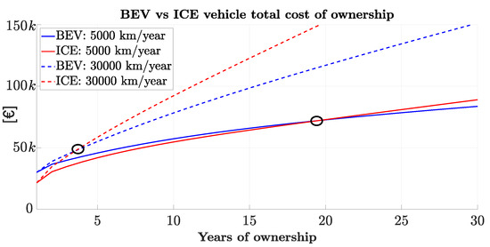
Figure 7.
Total cost of ownership of BEVs and ICEVs as a function of years of car ownership for varying annual mileages: 5000 km/year and 30,000 km/year in the high energy/fuel cost scenario.
5.3. Results of Merging the E-Mobility Index with Economics
We have now reached a point in the analysis where we can take the vehicles from our datasets (from the three provinces) that are functionally compatible with our home charging assumptions (which led to the quantification of the E-Mobility Index) and apply the economic arguments discussed above in the comparison between ICEVs and BEVs. The underlying assumption is that the cost scenario is simplified and uniformly applied to the two specific cars chosen for the comparison.
Figure 8 shows a picture of the TCO and its cost components in the second year of ownership for the two reference cars in the first economic scenario (high energy costs). In the upper panel, the BEV and ICEV TCOs are compared. Initially, the BEV TCO is higher due to the significant difference in purchase cost . In the lower panel, the weight of the various cost components over the total is shown.
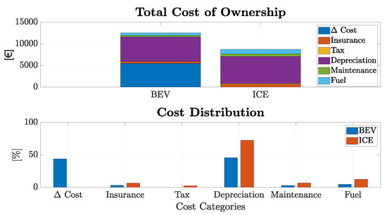
Figure 8.
TCO (upper panel) case in the second year of ownership for the reference BEV and ICEV in the sample case of a mileage of 10000 km/year and the impact of each cost component (lower panel).
Cross-referencing the functional feasibility (E-Private Mobility Index) and economic arguments, the resulting overall feasibility percentages are computed separately for the Bari, Brescia, and Rome provinces. Considering both the lower energy cost scenario ( EUR/KWh) and the higher one ( EUR/KWh) and processing the data relative to the already functionally feasible subsets of cars, Table 7 reports the fractions of these subsets for each province that, because of their yearly mileage driven, would break even in a maximum number of years . Clearly, sensitivity analysis could be conducted on this parameter as needed; however, for illustrative purposes, we have chosen to set years, since the average ownership period of a private car is seven and a half years in Italy; over the course of a lifetime, each person typically owns five different vehicles [39]. Seven and a half years may seem like a long period to some, but for many, it feels too short. However, it is likely that this time frame will extend further as the years go by. Within at most 8 years, , , and of the E-Private Mobility Index values identified private cars in Brescia, Rome, and Bari, respectively, that would reach the breakeven point when investing in a BEV and dismissing the current ICEVs (Figure 9).
Table 7.
E-Private Mobility Index with the breakeven time of years.
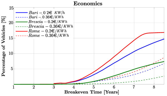
Figure 9.
Percentage of functionally compatible vehicles (thus included in the E-Mobility Index) as a function of the years required to break even considering the total cost of ownership separately for the three provinces of Brescia, Rome, and Bari, as well as in two different charging energy cost scenarios. In the Rome province, with energy priced at 0.2 EUR/kWh, which is the more affordable case, the solid-line graph clearly shows that all functionally compatible cars would also be economically compatible within 8 years. However, in Brescia and Bari, the percentage of functionally and economically compatible cars (thus included in the E-Mobility Index) grows more slowly, and breakeven is reached for all vehicles even beyond 8 years.
The very significant finding from these results is that, even under the assumption of low-cost home charging ( EUR/KWh), the percentage of current private cars that could realistically be replaced by the owner with a BEV, while maintaining the same travel habits and breaking even on the investment in a reasonable number of years, is very, very low. This percentage would become even lower, as seen in Table 7, assuming a higher energy cost ( EUR/KWh).
On the numbers in Table 7, it is worth making a more general but important observation. The three provinces’ behavior with respect to the obtained results varies significantly. However, in the provinces of Brescia and Bari, where the average annual distance traveled is lower because of their medium geographic extent, the absorption of excess car purchase cost is slower because the economic gain depends on the kilometers traveled. Therefore, although Brescia and Bari have a higher E-Private Mobility Index (thanks to the fact that there are fewer battery-range-exceeding trips), they turn out to have fewer cars that break even within 8 years, which is consistently due to the reduced average mileage per vehicle. On the contrary, Rome, which has a lower E-Private Mobility Index, exhibits a higher percentage of private cars that reach the breakeven point within 8 years due to the fact that, of the functionally feasible cars, a quite larger fraction drives for a greater mileage due to the province’s extent, resulting in a higher cost absorption rate.
6. Conclusions and Future Work
In the research described in this article, we aimed to provide a quantitative contribution to understanding the extent of fully electric vehicle penetration within the Italian car fleet, focusing specifically on three heterogeneous regions located in the north, center, and south of the country. We sought to answer the question of how many fully electric vehicles would presently be compatible with people’s driving habits in terms of trip lengths and stop durations, based not on models or surveys but on spatiotemporal GPS data from black boxes in hundreds of thousands of cars. Of course, the analysis is based on simplified yet reasonable assumptions, always taking a cautious approach regarding the range of the hypothetical BEVs and the availability of low-cost, home-based charging. To ensure clarity in the data analysis, we deliberately overlook several aspects in this initial study, such as the impact of environmental and structural factors on battery range and the existence of fast- or super-fast-charging stations, which remain scarce and expensive. These are factors that we plan to incorporate progressively in future developments of this work.
The dimensionality of the available telematic datasets ensures that the conclusions of this study are statistically relevant. The first significant result is that we synthesize an innovative indicator—the E-Private Mobility Index—measuring the percentage of private cars potentially ready to be substituted by fully electric ones, in the sense that their trips and stops over one year would be compatible with a feasible battery autonomy range and a home or a proximity recharging station. This measure of functional feasibility demonstrates that the Italian car fleet’s average percentage (each of the three regions is separately analyzed and considered in this study) of electrification feasibility is around , despite varying significantly from region to region. We then enhance the evaluation by cross-referencing the functional feasibility (E-Private Mobility Index) and economic arguments. The additional economic analysis aims at evaluating the breakeven time when purchasing a fully electric car (still more expensive) with respect to a traditional one. As the individual car ownership period in Italy is approximately 8 years, as a result, the percentage of functionally feasible cars (already included in the E-Mobility Index) could concretely reach the breakeven point within this reasonable number of years. By considering two energy cost scenarios, we show that, at the national level (each of the three regions is separately analyzed and considered in this study), about 15% of the circulating private cars make trips and stops compatible with the battery autonomy and recharging time on average; as such, the significantly higher purchase cost would be amortized over the considered period of time. A sensitivity analysis on the effect of considering government policies/incentives on the breakeven point would be a topic for future studies.
The key insight emerging from this data-driven analysis is that private fully electric vehicles need to be effectively driven over substantial distances and are naturally not easily compatible with private car ownership. For the reasons highlighted in this research based on real data, the vehicle fleet will continue to consist primarily of cars with internal combustion engines, for which it will be essential to adopt innovative monitoring systems at a vehicle level to individually assess emissions according to traveled distances, average speeds, and driving habits, rather than relying solely on average values from car manufacturers. It is clear that the BEV penetration estimates presented in this study may seem conservative, especially regarding the assumed battery range. Battery technology is evolving rapidly, and a greater range is now offered by recently produced BEVs. However, it is important to consider that the purchase cost of these vehicles remains high and increases significantly with higher battery capacity. Only Mobility as a Service (MaaS) and the shared use of fully electric autonomous vehicles will enable a fully electric mobility ecosystem. The number of privately owned cars will significantly decrease, at least in metropolitan areas, as people will rely on shared autonomous vehicles for necessary trips. These vehicles will be medium-sized, with a moderate range, traveling at “green” speeds. Most importantly, they will cover extensive distances, enabling both the previously discussed economic amortization and zero-emission operation while eliminating the need for public parking spaces. The anticipated transition to fully electric mobility will still need a few more years, but not too long, as autonomous vehicle technology—at least for supervised urban use at low speeds—is truly just around the corner.
7. Limitations
This study is based on several assumptions that future research may address in greater detail. In particular, the following limitations should be acknowledged:
- Infrastructure Scope: This study assumes that recharging occurs primarily at domestic or near-home locations. This assumption is supported by the current state of the charging network in Italy, where public infrastructure is still under development; in practice, the availability of a wall box or a semi-dedicated charging station at home almost always ensures a low-cost recharging option. However, the Italian charging network is not as widespread as those in some other European markets [40]. Consequently, the feasibility of BEVs might be underestimated if alternative charging scenarios (e.g., workplace or fast-charging stations) are considered.
- Data Scope: The analysis relied exclusively on telematic data provided by an Italian company. Consequently, the results are specific to the national context and may not be directly applicable to other European regions.
Author Contributions
Conceptualization, S.S. and S.M.S.; Methodology, S.S. and S.M.S.; Software, R.G.C. and A.P.; Validation, S.S. and R.G.C.; Formal analysis, S.S. and A.P.; Investigation, S.S. and R.G.C.; Data curation, R.G.C. and A.P.; Writing—original draft, S.S. and R.G.C.; Writing—review & editing, A.P.; Supervision, S.S. and S.M.S.; Project administration, S.S.; Funding acquisition, S.S. All authors have read and agreed to the published version of the manuscript.
Funding
This research received no external funding.
Institutional Review Board Statement
Not applicable.
Informed Consent Statement
Not applicable.
Data Availability Statement
The dataset used and analyzed in this study is not publicly available due to confidentiality agreements established under a funded research collaboration with the private telematics company UnipolTech Spa. As per the research contract, Politecnico di Milano is bound by a confidentiality clause restricting the disclosure of data, information, knowledge, and documents identified as confidential. However, a de-identified version of the comprehensive dataset will be provided by the corresponding author upon reasonable request.
Acknowledgments
We thank UnipolTech, a company of Unipol Group, for supporting this work by kindly making available a large quantity of mobility data from their insured vehicles’ telematic black boxes.
Conflicts of Interest
The authors declare no conflicts of interest.
References
- European Commission. European Green Deal. 2023. Available online: https://commission.europa.eu/strategy-and-policy/priorities-2019-2024/european-green-deal/transport-and-green-deal_en (accessed on 5 April 2025).
- European Parliament. EU Ban on Sale of New Petrol and Diesel Cars from 2035 Explained. 2022. Available online: https://www.europarl.europa.eu/topics/en/search?searchQuery=EU+Ban+on+Sale+of+New+Petrol+and+Diesel+Cars+from+2035+Explained (accessed on 5 April 2025).
- United Nations. Paris Agreement; United Nations: New York, NY, USA, 2015. [Google Scholar]
- European Environment Agency. Trends and Projections in Europe 2020—Tracking Progress Towards Europe’s Climate and Energy Targets; European Environment Agency: Copenhagen, Denmark, 2020. [Google Scholar]
- European Commission. A Clean Planet for All—A European Strategic Long-Term Vision for a Prosperous, Modern, Competitive and Climate Neutral Economy; European Commission: Brussel, Belgium, 2018. [Google Scholar]
- Maybury, L.; Corcoran, P.; Cipcigan, L. Mathematical modelling of electric vehicle adoption: A systematic literature review. Transp. Res. Part D Transp. Environ. 2022, 107, 103278. [Google Scholar] [CrossRef]
- Slowik, P.; Lutsey, N. The continued transition to electric vehicles in US cities. In White Paper; The International Council of Clean Transportation (ICCT): Washington, DC, USA, 2018. [Google Scholar]
- Needell, Z.A.; McNerney, J.; Chang, M.T.; Trancik, J.E. Potential for widespread electrification of personal vehicle travel in the United States. Nat. Energy 2016, 1, 16112. [Google Scholar] [CrossRef]
- Stokes, L.C.; Breetz, H.L. Politics in the US energy transition: Case studies of solar, wind, biofuels and electric vehicles policy. Energy Policy 2018, 113, 76–86. [Google Scholar] [CrossRef]
- Holland, S.P.; Mansur, E.T.; Yates, A.J. The electric vehicle transition and the economics of banning gasoline vehicles. Am. Econ. J. Econ. Policy 2021, 13, 316–344. [Google Scholar] [CrossRef]
- Lutsey, N. Global climate change mitigation potential from a transition to electric vehicles. Int. Counc. Clean Transp. 2015, 5, 5. [Google Scholar]
- Hardman, S.; Fleming, K.L.; Khare, E.; Ramadan, M.M. A perspective on equity in the transition to electric vehicle. MIT Sci. Policy Rev. 2021, 2, 46–54. [Google Scholar] [CrossRef]
- Dall-Orsoletta, A.; Ferreira, P.; Gilson Dranka, G. Low-carbon technologies and just energy transition: Prospects for electric vehicles. Energy Convers. Manag. X 2022, 16, 100271. [Google Scholar] [CrossRef]
- Riesz, J.; Sotiriadis, C.; Ambach, D.; Donovan, S. Quantifying the costs of a rapid transition to electric vehicles. Appl. Energy 2016, 180, 287–300. [Google Scholar] [CrossRef]
- Chaturvedi, B.; Nautiyal, A.; Kandpal, T.; Yaqoot, M. Projected transition to electric vehicles in India and its impact on stakeholders. Energy Sustain. Dev. 2022, 66, 189–200. [Google Scholar] [CrossRef]
- Hsieh, I.Y.L.; Pan, M.S.; Green, W.H. Transition to electric vehicles in China: Implications for private motorization rate and battery market. Energy policy 2020, 144, 111654. [Google Scholar] [CrossRef]
- Zinnari, F.; Strada, S.; Tanelli, M.; Formentin, S.; Savaresi, S.M. Electrification potential of fuel-based vehicles and optimal placing of charging infrastructure: A large-scale vehicle-telematics approach. IEEE Trans. Transp. Electrif. 2021, 8, 466–479. [Google Scholar] [CrossRef]
- De Gennaro, M.; Paffumi, E.; Martini, G.; Scholz, H. A pilot study to address the travel behaviour and the usability of electric vehicles in two Italian provinces. Case Stud. Transp. Policy 2014, 2, 116–141. [Google Scholar] [CrossRef]
- Roblek, V.; Meško, M.; Podbregar, I. Impact of Car Sharing on Urban Sustainability. Sustainability 2021, 13, 905. [Google Scholar] [CrossRef]
- Machado, C.A.S.; de Salles Hue, N.P.M.; Berssaneti, F.T.; Quintanilha, J.A. An overview of shared mobility. Sustainability 2018, 10, 4342. [Google Scholar] [CrossRef]
- Sheldon, T.L.; Dua, R. Consumer preferences for ride-hailing: Barriers to an autonomous, shared, and electric future. J. Clean. Prod. 2024, 434, 140251. [Google Scholar] [CrossRef]
- Pezoa, R.; de Grange, L.; Troncoso, R. Paying to depollute: The case of electric ride-hailing. Resour. Energy Econ. 2025, 82, 101478. [Google Scholar] [CrossRef]
- Taiebat, M.; Xu, M. Synergies of four emerging technologies for accelerated adoption of electric vehicles: Shared mobility, wireless charging, vehicle-to-grid, and vehicle automation. J. Clean. Prod. 2019, 230, 794–797. [Google Scholar] [CrossRef]
- Ball, S.; Cairns, S.; Emmerson, P.; Wilson, R.; Anable, J.; Chatterton, T. Understanding Variation in Car Use: Exploration of Statistical Metrics at Differing Spatial Scales Using Data from Every Private Car Registered in Great Britain; Transport Research Laboratory: Omaha, NE, USA, 2016. [Google Scholar]
- Le Duigou, A.; Guan, Y.; Amalric, Y. On the competitiveness of electric driving in France: Impact of driving patterns. Renew. Sustain. Energy Rev. 2014, 37, 348–359. [Google Scholar] [CrossRef]
- Jensen, A.F.; Cherchi, E.; Mabit, S.L. On the stability of preferences and attitudes before and after experiencing an electric vehicle. Transp. Res. Part D Transp. Environ. 2013, 25, 24–32. [Google Scholar] [CrossRef]
- Plötz, P.; Schneider, U.; Globisch, J.; Dütschke, E. Who will buy electric vehicles? Identifying early adopters in Germany. Transp. Res. Part A Policy Pract. 2014, 67, 96–109. [Google Scholar] [CrossRef]
- Robusto, C. The cosine-haversine formula. Am. Math. Mon. 1957, 64, 38–40. [Google Scholar] [CrossRef]
- Monawar, T.; Mahmud, S.B.; Hira, A. Anti-theft vehicle tracking and regaining system with automatic police notifying using Haversine formula. In Proceedings of the 2017 4th International Conference on Advances in Electrical Engineering (ICAEE), Dhaka, Bangladesh, 28–30 September 2017; IEEE: Piscataway, NJ, USA, 2017; pp. 775–779. [Google Scholar]
- Sofwan, A.; Soetrisno, Y.A.A.; Ramadhani, N.P.; Rahmayani, A.; Handoyo, E.; Arfan, M. Vehicle distance measurement tuning using Haversine and micro-segmentation. In Proceedings of the 2019 International Seminar on Intelligent Technology and Its Applications (ISITIA), Surabaya, Indonesia, 28–29 August 2019; IEEE: Piscataway, NJ, USA, 2019; pp. 239–243. [Google Scholar]
- Schubert, E.; Sander, J.; Ester, M.; Kriegel, H.P.; Xu, X. DBSCAN revisited, revisited: Why and how you should (still) use DBSCAN. ACM Trans. Database Syst. (TODS) 2017, 42, 1–21. [Google Scholar] [CrossRef]
- Dericioglu, C.; Yirik, E.; Unal, E.; Cuma, M.U.; Onur, B.; Tumay, M. A review of charging technologies for commercial electric vehicles. Int. J. Adv. Automot. Technol. 2018, 2, 61–70. [Google Scholar]
- He, W.; Williard, N.; Chen, C.; Pecht, M. State of charge estimation for electric vehicle batteries using unscented kalman filtering. Microelectron. Reliab. 2013, 53, 840–847. [Google Scholar] [CrossRef]
- Tran, M.K.; Bhatti, A.; Vrolyk, R.; Wong, D.; Panchal, S.; Fowler, M.; Fraser, R. A review of range extenders in battery electric vehicles: Current progress and future perspectives. World Electr. Veh. J. 2021, 12, 54. [Google Scholar] [CrossRef]
- Ferriani, F.; Gazzani, A. The impact of the war in Ukraine on energy prices: Consequences for firms’ financial performance. Int. Econ. 2023, 174, 221–230. [Google Scholar] [CrossRef]
- Khudaykulova, M.; Yuanqiong, H.; Khudaykulov, A. Economic consequences and implications of the Ukraine-russia war. Int. J. Manag. Sci. Bus. Adm. 2022, 8, 44–52. [Google Scholar] [CrossRef]
- Roeger, W.; Welfens, P.J. Gas price caps and electricity production effects in the context of the Russo-Ukrainian War: Modeling and new policy reforms. Int. Econ. Econ. Policy 2022, 19, 645–673. [Google Scholar] [CrossRef]
- Burnham, A.; Gohlke, D.; Rush, L.; Stephens, T.; Zhou, Y.; Delucchi, M.; Birky, A.; Hunter, C.; Lin, Z.; Ou, S.; et al. Comprehensive Total Cost of Ownership Quantification for Vehicles with Different Size Classes and Powertrains; Argonne National Lab.(ANL): Argonne, IL, USA, 2021. [Google Scholar]
- EveryEyeAuto.it. Ogni Quanti Anni un Italiano Cambia la Propria Auto? Meno di Quanto Pensiate. 2023. Available online: https://auto.everyeye.it/notizie/anni-italiano-cambia-propria-auto-pensiate-634541.html (accessed on 5 April 2025).
- New Study on Accelerating EU Electric Vehicle Charging Infrastructure Roll-Out; Technical Report; European Commission: Brussel, Belgium, 2024.
Disclaimer/Publisher’s Note: The statements, opinions and data contained in all publications are solely those of the individual author(s) and contributor(s) and not of MDPI and/or the editor(s). MDPI and/or the editor(s) disclaim responsibility for any injury to people or property resulting from any ideas, methods, instructions or products referred to in the content. |
© 2025 by the authors. Licensee MDPI, Basel, Switzerland. This article is an open access article distributed under the terms and conditions of the Creative Commons Attribution (CC BY) license (https://creativecommons.org/licenses/by/4.0/).