
Impacts of Hydrothermal Factors on the Spatiotemporal Dynamics of Alpine Grassland Aboveground Biomass During the Pre-, Mid-, and Post-COVID-19 Pandemic Periods

 , , , , , and
Abstract
1. Introduction
2. Materials and Methods
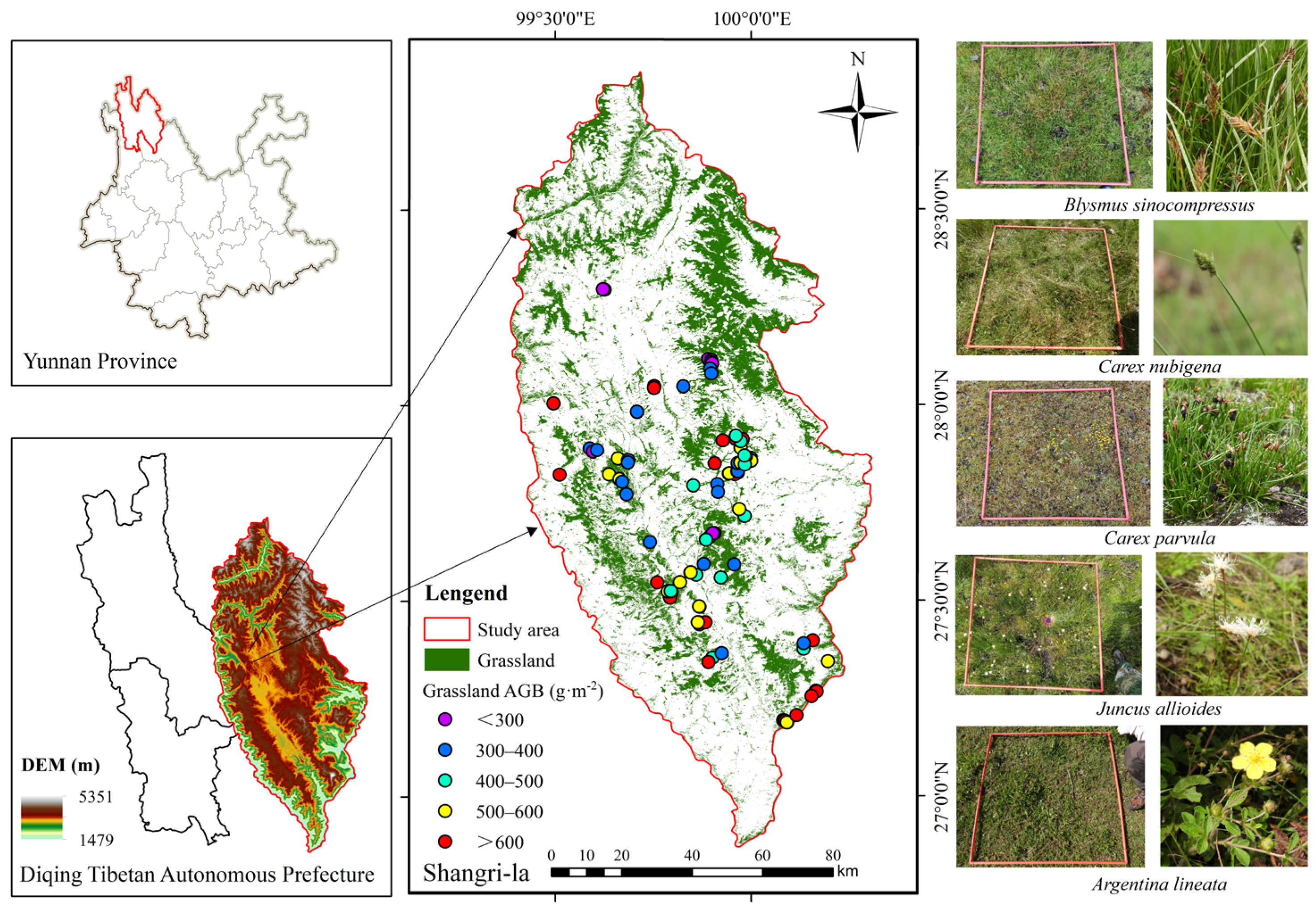
2.1. Study Area
2.2. Data Collection
2.2.1. Field Survey Data
2.2.2. Remote Sensing Data
2.2.3. Other Data
2.3. Data Analysis
2.3.1. Biomass Estimation
2.3.2. Biomass Trend
2.3.3. Response to Hydrothermal Factors
2.3.4. The Indirect Impact of the COVID-19 Pandemic
3. Results
3.1. Biomass Estimation
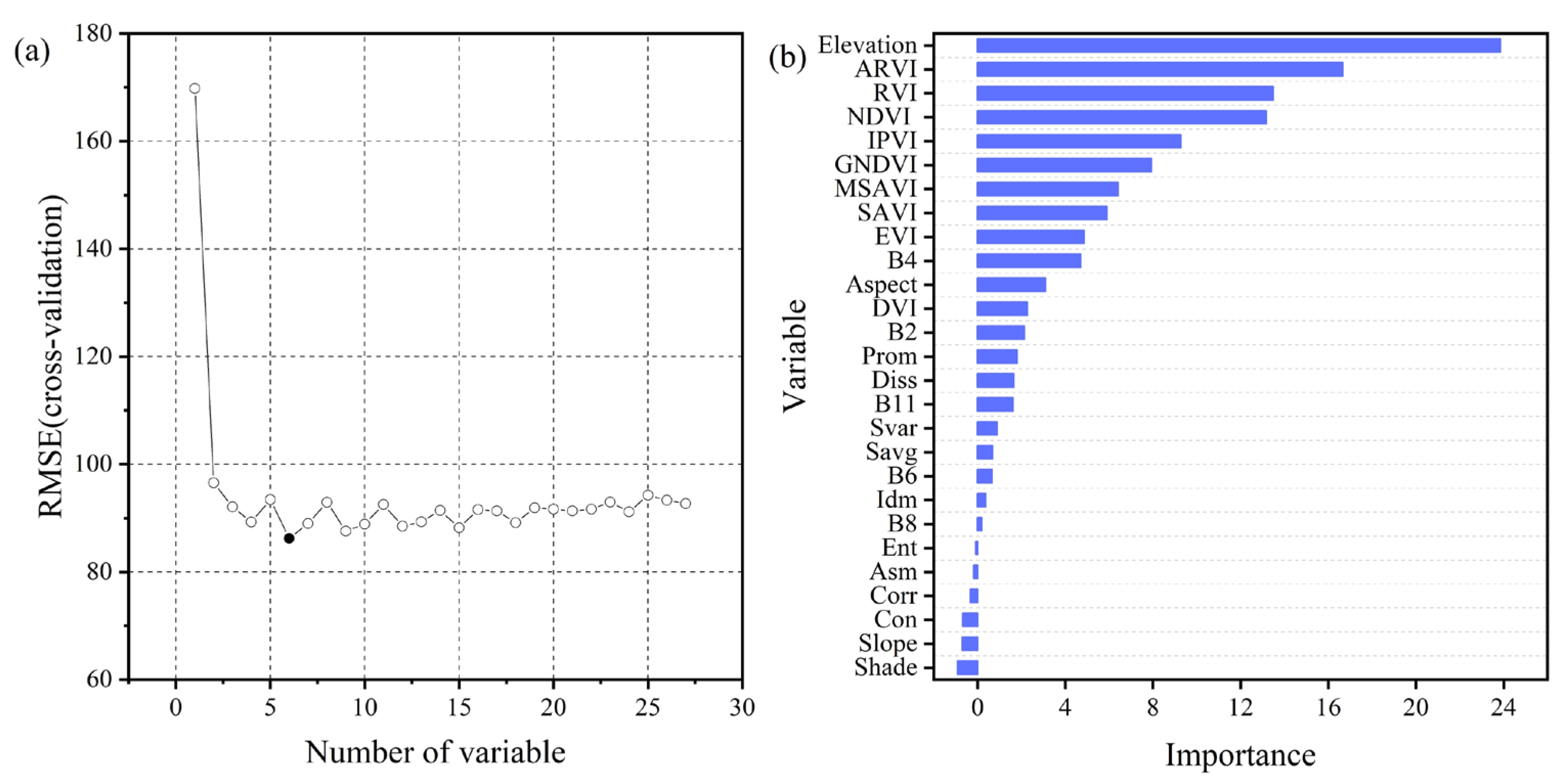
3.1.1. Optimization of Machine-Learning Models
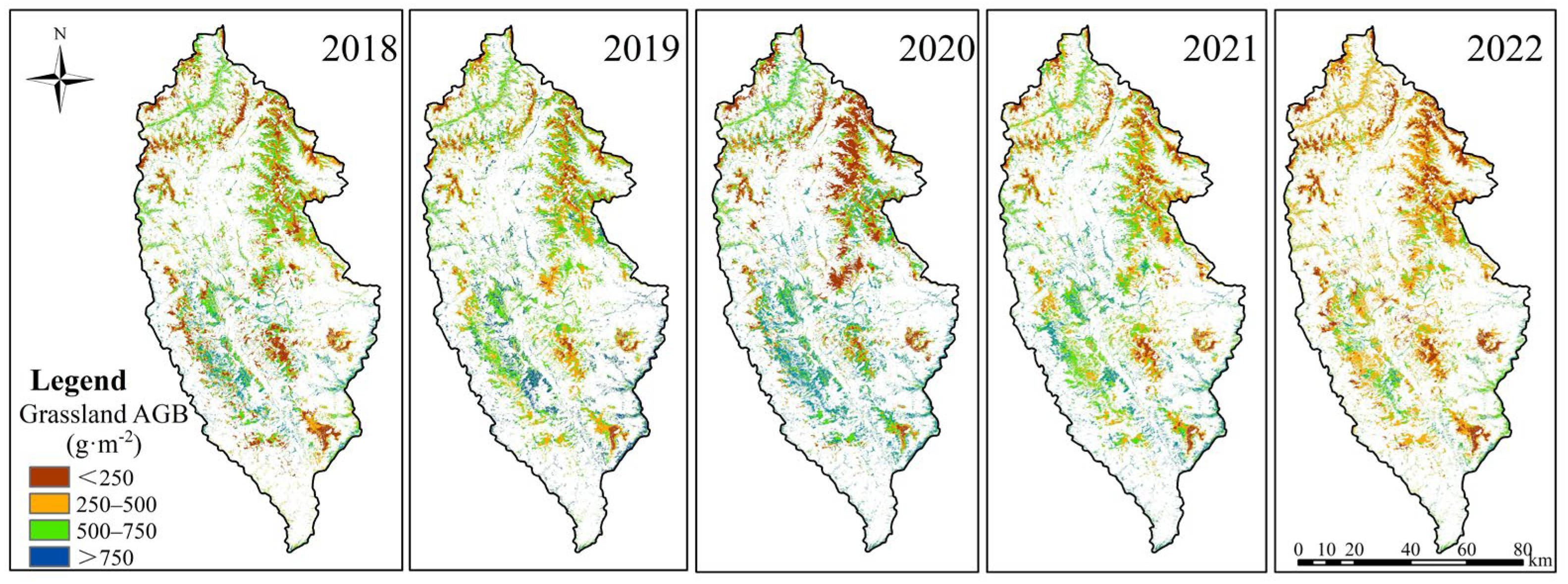
3.1.2. Spatial Distribution and Interannual Dynamics
3.2. Biomass Trend
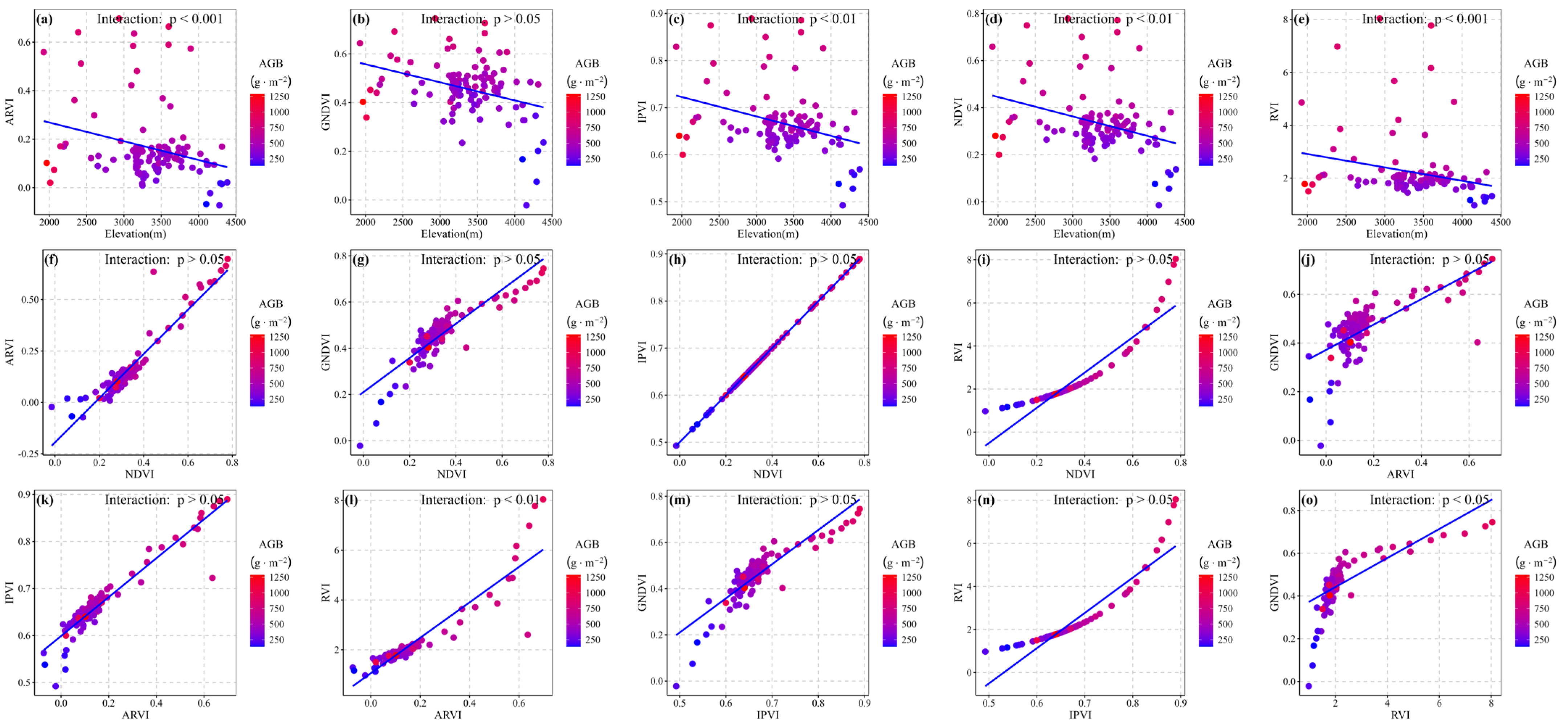
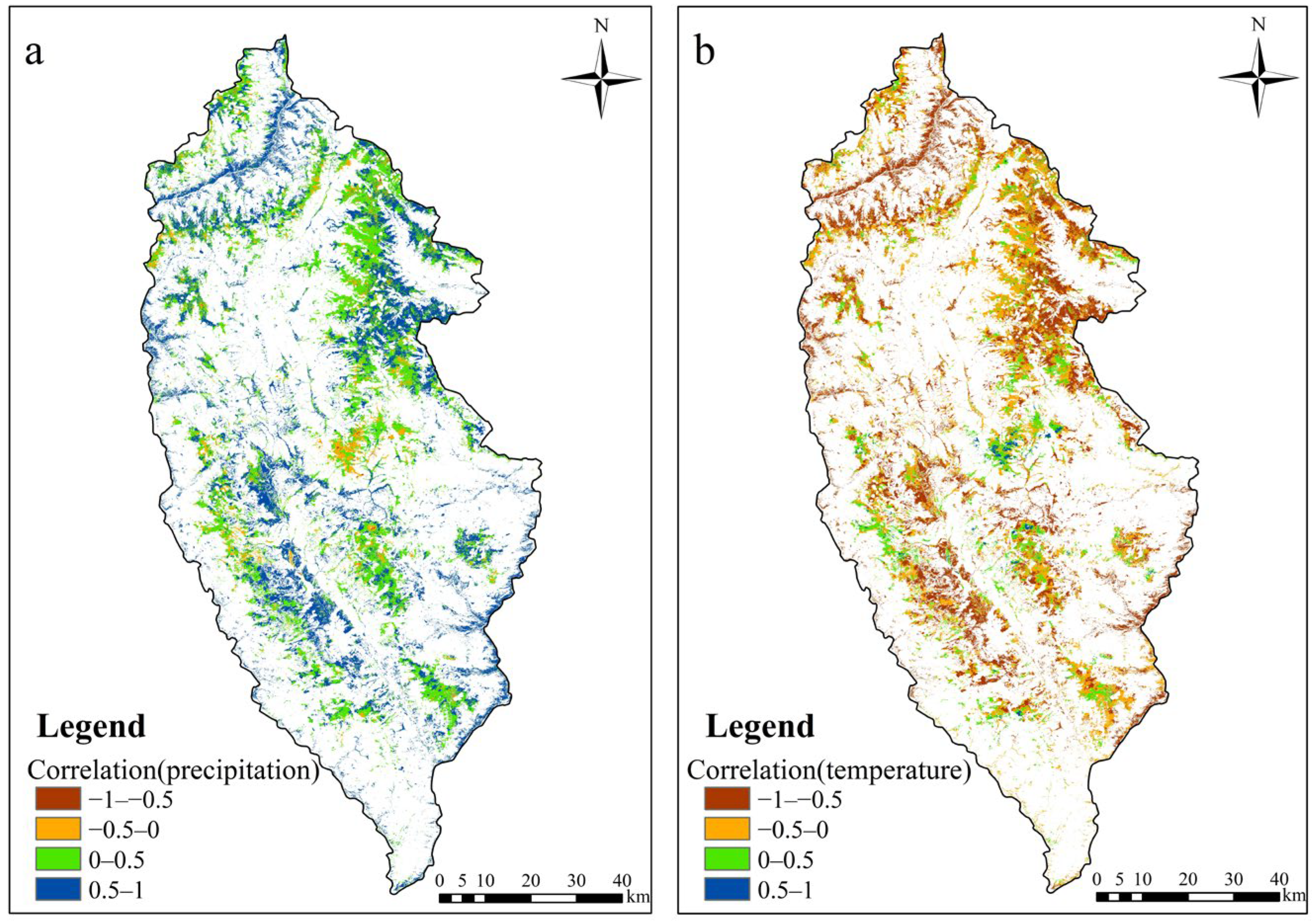
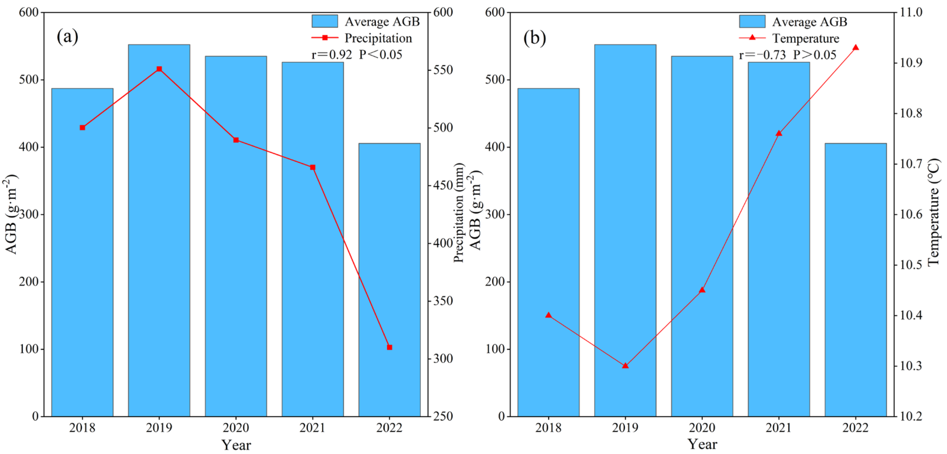
3.3. Response to Hydrothermal Factors
3.4. The Potential Impact of the Pandemic
4. Discussion
4.1. Performance of Machine-Learning Algorithms for Biomass Estimation
4.2. Trend of Grassland AGB
4.3. Relationships Between AGB and Hydrothermal Factors
4.4. The Potential Impact of the COVID-19 Pandemic
5. Conclusions
Supplementary Materials
Author Contributions
Funding
Institutional Review Board Statement
Informed Consent Statement
Data Availability Statement
Acknowledgments
Conflicts of Interest
Abbreviations
| AGB | Aboveground biomass |
| RF | Random forest |
| SVM | Support vector machine |
| ANN | Artificial neural network |
| GPR | Gaussian process regression |
Appendix A

| Variables | Equations |
|---|---|
| Normalized difference vegetation index (NDVI) | |
| Ratio vegetation index (RVI) | RVI = B8/B4 |
| Difference vegetation index (DVI) | DVI = B8 − B4 |
| Enhanced vegetation index (EVI) | |
| Soil adjusted vegetation index (SAVI) | |
| Modified soil adjusted vegetation index (MSAVI) | |
| Atmospherically resistant vegetation index (ARVI) | ARVI = B8 − (2 × B4 − B2)/B8 + (2 × B4 − B2) |
| NDVI of green band (GNDVI) | |
| Infrared vegetation index (IPVI) | IPVI = B8/(B8+B4) |
| Sum average (Savg) | |
| Angular second moment (Asm) | |
| Correlation (Corr) | |
| Inverse difference moment (Idm) | |
| Entropy (Ent) | |
| Shade (Cluster Shade) | |
| Dissimilarity (Diss) | |
| Sum variance (Svar) | |
| Cluster prominence (Prom) | |
| Contrast (Con) |
References
- Sun, J.; Wang, Y.; Piao, S.L.; Liu, M.; Han, G.D.; Li, J.R.; Liang, E.Y.; Lee, T.M.; Liu, G.H.; Wilkes, A.; et al. Toward a sustainable grassland ecosystem worldwide. Innovation 2022, 3, 100265. [Google Scholar] [CrossRef] [PubMed]
- Lewińska, K.E.; Ives, A.R.; Morrow, C.J.; Rogova, N.; Yin, H.; Elsen, P.R.; de Beurs, K.; Hostert, P.; Radeloff, V.C. Beyond “greening” and “browning”: Trends in grassland ground cover fractions across Eurasia that account for spatial and temporal autocorrelation. Global Change Biol. 2023, 29, 4620–4637. [Google Scholar] [CrossRef] [PubMed]
- Enquist, B.J.; Niklas, K.J. Global Allocation Rules for Patterns of Biomass Partitioning in Seed Plants. Science 2002, 295, 1517–1520. [Google Scholar] [CrossRef]
- Buisson, E.; Archibald, S.; Fidelis, A.; Suding, K.N. Ancient grassland guide ambitious goals in grassland recovery. Science 2022, 377, 594–598. [Google Scholar] [CrossRef]
- Dong, P.; Jang, C.J.; Wang, G.X.; Shao, Y.Q.; Gao, Y.Z. The Estimation of Grassland Aboveground Biomass and Analysis of Its Response to Climatic Factors Using a Random Forest Algorithm in Xinjiang, China. Plants 2024, 13, 548. [Google Scholar] [CrossRef]
- Luo, R.; Yang, S.L.; Zhou, Y.; Gao, P.Q.; Zhang, T.M. Spatial Pattern Analysis of a Water-Related Ecosystem Service and Evaluation of the Grassland-Carrying Capacity of the Heihe River Basin under Land Use Change. Water 2021, 13, 2658. [Google Scholar] [CrossRef]
- Wang, S.S.; Dai, E.F.; Jia, L.Z.; Wang, Y.J.; Huang, A.Q.; Liao, L.; Cai, L.P.; Fan, D.G. Assessment of multiple factors and interactions affecting grassland degradation on the Tibetan Plateau. Ecol. Indic. 2023, 154, 110509. [Google Scholar] [CrossRef]
- Joseph, G.S.; Seymour, C.L.; Rakotoarivelo, A.R. Fire incongruities can explain widespread landscape degradation in Madagascar’s forests and grasslands. Plants People Planet 2024, 6, 656–669. [Google Scholar] [CrossRef]
- Su, F.Z.; Fu, D.J.; Yan, F.Q.; Han, X.; Pan, T.T.; Xiao, Y.; Kang, L.; Zhou, C.H.; Meadows, M.; Lyne, V.; et al. Rapid greening response of China’s 2020 spring vegetation to COVID-19 restrictions: Implications for climate change. Sci. Adv. 2021, 7, eabe8044. [Google Scholar]
- Dang, C.Y.; Shao, Z.F.; Huang, X.; Zhuang, Q.W.; Cheng, G.; Qian, J.X. Global vegetation productivity increased in response COVID-19 restrictions. Geo-Spa. Inf. Sci. 2024, 27, 2123–2136. [Google Scholar] [CrossRef]
- Yuan, Y.X.; Wen, Q.K.; Zhao, X.L.; Liu, S.; Zhu, K.P.; Hi, B. Identifying Grassland Distribution in a Mountainous Region in Southwest China Using Multi-Source Remote Sensing Images. Remote. Sens. 2022, 14, 1472. [Google Scholar] [CrossRef]
- Ge, J.; Hou, M.J.; Liang, T.G.; Feng, Q.S.; Meng, X.Y.; Liu, J.; Bao, X.Y.; Gao, H.Y. Spatiotemporal dynamics of grassland aboveground biomass and its driving factors in North China over the past 20 years. Sci. Total. Environ. 2022, 826, 154226. [Google Scholar] [CrossRef] [PubMed]
- Zhou, Y.; Cui, S.J.; Lv, W.W.; Sun, J.P.; Lv, J.Y.; Li, B.W.; Chen, L.Y.; Dorji, T.; Wang, S.P. Warming neither accelerates degradation of alpine grasslands nor promotes recovery of degraded alpine grasslands on the Tibetan Plateau. Catena 2024, 242, 108102. [Google Scholar] [CrossRef]
- Morais, T.G.; Teixeira, R.F.; Figueiredo, M.; Domingos, T. The use of machine learning methods to estimate aboveground biomass of grasslands: A review. Ecol. Indic. 2021, 130, 108081. [Google Scholar] [CrossRef]
- Marino, S.; Brugiapaglia, E.; Miraglia, N.; Persichili, C.; Angelis, M.D.; Pilla, F.; Brita, A.D. Modelling of the above-ground biomass and ecological composition of semi-natural grasslands on the strength of remote sensing data and machine learning algorithms. Ecol. Inform. 2024, 82, 102740. [Google Scholar] [CrossRef]
- Gao, X.X.; Dong, S.K.; Li, S.; Xu, Y.D.; Liu, S.L.; Zhao, H.D.; Yeomans, J.; Li, Y.; Shen, H.; Wu, S.N.; et al. Using the random forest model and validated MODIS with the field spectrometer measurement promote the accuracy of estimating aboveground biomass and coverage of alpine grasslands on the Qinghai-Tibetan Plateau. Ecol. Indic. 2020, 112, 106114. [Google Scholar] [CrossRef]
- Liu, W.J.; Xu, C.; Zhang, Z.M.; Boeck, H.D.; Wang, Y.F.; Zhang, L.K.; Xu, X.G.; Zhang, C.; Chen, G.R.; Xu, C. Machine learning-based grassland aboveground biomass estimation and its response to climate variation in Southwest China. Front. Ecol. Evol. 2023, 11, 1146850. [Google Scholar] [CrossRef]
- John, R.; Chen, J.Q.; Giannico, V.; Park, H.; Xiao, J.F.; Shirkey, G.; Ouyang, Z.; Shao, C.L.; Lafortezza, R.; Qi, J.G. Grassland canopy cover and aboveground biomass in Mongolia and Inner Mongolia: Spatiotemporal estimates and controlling factors. Remote. Sens. Environ. 2018, 213, 34–48. [Google Scholar] [CrossRef]
- Zeng, N.; Ren, X.L.; He, H.L.; Zhang, L.; Li, P.; Niu, Z.G. Estimating the grassland aboveground biomass in the Three-River Headwater Region of China using machine learning and Bayesian model averaging. Environ. Res. Lett. 2021, 16, 114020. [Google Scholar]
- Yang, Y.H.; Fang, J.Y.; Ma, W.H.; Wang, W. Relationship between variability in aboveground net primary production and precipitation in global grasslands. Geophys. Res. Lett. 2008, 35, L23710. [Google Scholar] [CrossRef]
- He, H.; Yu, H.; Rong, Z.W.; Yang, Y.; Li, P.S. Estimation of grassland aboveground biomass and its response to climate changes based on remote sensing inversion in Three-River-Source National Park, Tibet Plateau, China. Front. Ecol. Evol. 2023, 11, 1326980. [Google Scholar] [CrossRef]
- Wang, Q.; Su, M. A preliminary assessment of the impact of COVID-19 on environment-A case study of China. Sci. Total Environ. 2020, 728, 138915. [Google Scholar] [CrossRef] [PubMed]
- Mofijur, M.; Fattah, I.M.R.; Alam, M.A.; Islam, A.B.M.S.; Ong, H.C.; Rahman, S.M.A.; Najafi, G.; Ahmed, S.F.; Uddin, N.A.; Mahlia, T.M.I. Impact of COVID-19 on the social, economic environmental and energy domains: Lessons learnt from a global pandemic. Sustain. Prod. Consum. 2021, 26, 343–359. [Google Scholar] [CrossRef]
- Miyah, Y.; Benjelloun, M.; Lairini, S.; Lahrichi, A. COVID-19 impact on public health, environment, human psychology, global socioeconomy, and education. Sci. World J. 2022, 2022, 5578284. [Google Scholar] [CrossRef] [PubMed]
- Boval, M.; Dixon, R.M. The importance of grasslands for animal production and other functions: A review on management and methodological progress in the tropics. Animal 2012, 6, 748–762. [Google Scholar] [CrossRef]
- Tindale, S.; Vicario-Modroño, V.; Gallardo-Cobos, R.; Hunter, E.; Miškolci, S.; Price, P.N.; Sánchez-Zamora, P.; Sonnevelt, M.; Ojo, M.; McInnes, K.; et al. Citizen perceptions and values associated with ecosystem services from European grassland landscapes. Land. Use Policy 2023, 127, 106574. [Google Scholar] [CrossRef]
- Yin, C.X.; Qin, S.M. Personal Factors Influencing Pro-environmental Behavioral Intentions of Tourists in National Parks: A Case Study of the Potatso National Park. J. Beijing For. Univ. 2023, 22, 32–34. [Google Scholar]
- Gibbons, D.W.; Sandbrook, C.; Sutherland, W.J.; Akter, R.; Bradbury, R.; Broad, S.; Crick, H.Q.; Elliott, J.; Gyeltshen, N.; Heath, M. The relative importance of COVID-19 pandemic impacts on biodiversity conservation globally. Conserv. Biol. 2022, 36, e13781. [Google Scholar] [CrossRef]
- Kashyap, R.; Kuttippurath, J.; Patel, V.K. Improved air quality leads to enhanced vegetation growth during the COVID-19 lockdown in India. Appl. Geogr. 2022, 151, 102869. [Google Scholar] [CrossRef]
- Yang, Y.L.; Wang, J.L.; Chen, Y.; Cheng, F.; Liu, G.J.; He, Z.H. Remote-Sensing Monitoring of Grassland Degradation Based on the GDI in Shangri-La, China. Remote Sens. 2019, 11, 3030. [Google Scholar] [CrossRef]
- Chang, C.; Chang, Y.; Xiong, Z.P.; Liu, H.S.; Bu, R.C. Estimating the aboveground biomass of the Hulunbuir Grassland and exploring its spatial and temporal variations over the past ten years. Ecol. Indic. 2024, 161, 112010. [Google Scholar] [CrossRef]
- Luo, Z.X.; Deng, L.; Yan, C.Z. Soil erosion under different plant cover types and its influencing factors in Napahai Catchment, Shangri-La County, Yunnan Province, China. Int. J. Sustain. Dev. World Ecol. 2015, 22, 135–141. [Google Scholar] [CrossRef]
- Cai, T.Y.; Chang, C.C.; Zhao, Y.B.; Wang, X.; Yang, J.L.; Dou, P.P.; Otgonbayar, M.; Zhang, G.L.; Zeng, Y.L.; Wang, J. Within-season estimates of 10 m aboveground biomass based on Landsat, Sentinel-2 and PlanetScope data. Sci. Data 2024, 23, 1276. [Google Scholar] [CrossRef] [PubMed]
- Li, M.; Wu, J.S.; Song, C.Q.; He, Y.T.; Niu, B.; Fu, G.; Tarolli, P.; Tietjen, B.; Zhang, X.Z. Temporal variability of precipitation and biomass of alpine grasslands on the northern Tibetan plateau. Remote Sens. 2019, 3, 360. [Google Scholar] [CrossRef]
- Yang, Y.; Dou, Y.X.; An, S.S. Environmental driving factors affecting plant biomass in natural grassland in the Loess Plateau, China. Ecol. Indic. 2017, 82, 250–259. [Google Scholar] [CrossRef]
- Wu, N.; Liu, G.X.; Wuyun, D.J.; Yi, B.L.; Du, W.L.; Han, G.D. Spatial-temporal characteristics and driving forces of aboveground biomass in desert steppes of inner Mongolia, China in the past 20 years. Remote Sens. 2023, 15, 3097. [Google Scholar] [CrossRef]
- Lv, J.X.; Zhao, W.W.; Hua, T.; Zhang, L.H.; Pereira, P. Multiple Greenness Indexes revealed the vegetation greening during the growing season and winter on the Tibetan Plateau despite regional variations. Remote Sens. 2023, 15, 5679. [Google Scholar] [CrossRef]
- Liu, E.Q.; Zhou, W.C.; Zhou, J.M.; Shao, H.Y.; Yang, X. Combining Spectral with Texture Features into Object- oriented Classification in Mountainous Terrain Using Advanced Land Observing Satellite Image. J. Mt. Sci. 2013, 10, 768–776. [Google Scholar] [CrossRef]
- Funk, C.; Peterson, P.; Landsfeld, M.; Pedreros, D.; Verdin, J.; Shukla, S.; Husak, G.; Rowland, J.; Harrison, L.; Hoell, A.; et al. The climate hazards infrared precipitation with stations-a new environmental record for monitoring extremes. Sci. Data 2015, 2, 150066. [Google Scholar] [CrossRef]
- Peng, S.Z.; Ding, Y.X.; Liu, W.Z.; Li, Z. 1 km monthly temperature and precipitation dataset for China from 1901 to 2017. Earth. Syst. Sci. Data 2019, 11, 1931–1946. [Google Scholar] [CrossRef]
- Wang, Y.Y.; Wu, G.L.; Deng, L.; Tang, Z.S.; Wang, K.B.; Sun, W.Y.; Shangguan, Z.P. Prediction of aboveground grassland biomass on the Loess Plateau, China, using a random forest algorithm. Sci. Rep. 2017, 7, 6940. [Google Scholar] [CrossRef] [PubMed]
- Ren, J.H.; Cai, J.F.; Li, J.J. High precision implicit function learning for forecasting supercapacitor state of health based on Gaussian process regression. Sci. Rep. 2021, 11, 12112. [Google Scholar] [CrossRef] [PubMed]
- Huang, W.Y.; Li, W.L.; Xu, J.; Ma, X.L.; Li, C.H.; Liu, C.L. Hyperspectral Monitoring Driven by Machine Learning Methods for Grassland Above-Ground Biomass. Remote Sens. 2022, 14, 2086. [Google Scholar] [CrossRef]
- Pan, G.Z.; Yang, M.; Zhou, J.; Yuan, H.; Miao, C.; Zhang, G. Quantifying entanglement for unknown quantum states via artificial neural networks. Sci. Rep. 2024, 14, 26267. [Google Scholar] [CrossRef]
- Mao, Y.; Pi, D.Y.; Liu, Y.M.; Sun, Y.X. Accelerated Recursive Feature Elimination Based on Support Vector Machine for Key Variable Identification. Chin. J. Chem. Eng. 2006, 14, 65–72. [Google Scholar] [CrossRef]
- Zhang, Y.Z.; Ma, J.; Liang, S.L.; Li, X.S.; Liu, J.D. A stacking ensemble algorithm for improving the biases of forest aboveground biomass estimations from multiple remotely sensed datasets. GIsci. Remote Sens. 2022, 59, 234–249. [Google Scholar] [CrossRef]
- Liu, S.L.; Cheng, F.Y.; Dong, S.K.; Zhao, H.D.; Hou, X.Y.; Wu, X. Spatiotemporal dynamics of grassland aboveground biomass on the Qinghai-Tibet Plateau based on validated MODIS NDVI. Sci. Rep. 2017, 7, 4182. [Google Scholar] [CrossRef]
- Ding, L.; Li, Z.W.; Shen, B.B.; Wang, X.; Xu, D.W.; Yan, R.R.; Yan, Y.C.; Xin, X.P.; Xiao, J.F.; Li, M.; et al. Spatial patterns and driving factors of aboveground and belowground biomass over the eastern Eurasian steppe. Sci. Total Environ. 2022, 803, 149700. [Google Scholar] [CrossRef]
- Jiang, W.G.; Yuan, L.H.; Wang, W.J.; Cao, R.; Zhang, Y.F.; Shen, W.N. Spatio-temporal analysis of vegetation variation in the Yellow River Basin. Ecol. Indic. 2015, 51, 117–126. [Google Scholar] [CrossRef]
- Zhong, F. Atheoretical approach based on machine learning for estimation of physical properties of LLDPE in moulding process. Sci. Rep. 2024, 14, 22119. [Google Scholar] [CrossRef]
- Buda, A.R.; Millar, D.J.; Kennedy, C.D.; Welsh, M.K.; Wiegman, A.R. Trends in extreme rainfall over the past 55 years suggest springtime subhourly rainfall extremes have intensified in Mahantango Creek, Pennsylvania. Sci. Rep. 2024, 14, 27837. [Google Scholar] [CrossRef] [PubMed]
- Peng, J.; Liu, Z.H.; Liu, Y.G.; Wu, J.S.; Han, Y.N. Trend analysis of vegetation dynamics in Qinghai–Tibet Plateau using Hurst Exponent. Ecol. Indic. 2012, 14, 28–39. [Google Scholar] [CrossRef]
- Lyu, X.; Li, X.B.; Gong, J.R.; Li, S.K.; Dou, H.S.; Dang, D.L.; Xuan, X.J.; Wang, H. Remote-sensing inversion method for aboveground biomass of typical steppe in Inner Mongolia, China. Ecol. Indic. 2021, 120, 106883. [Google Scholar] [CrossRef]
- Bu, L.X.; Lai, Q.; Qing, S.; Bao, Y.H.; Liu, X.Y.; Na, Q.; Li, Y. Grassland Biomass Inversion Based on a Random Forest Algorithm and Drought Risk Assessment. Remote Sens. 2022, 14, 5745. [Google Scholar] [CrossRef]
- Dusseux, P.; Guyet, T.; Pattier, P.; Barbier, V.; Nicolas, H. Monitoring of grassland productivity using Sentinel-2 remote sensing data. Int. J. Appl. Earth Obs. Geoinf. 2022, 111, 102843. [Google Scholar]
- Riihimäki, H.; Heiskanen, J.; Luoto, M. The effect of topography on arctic-alpine aboveground biomass and NDVI patterns. Int. J. Appl. Earth Obs. Geoinf. 2017, 56, 44–53. [Google Scholar]
- Meng, M.H.; Zhao, C.F. Application of support vector machines to a small-sample prediction. Adv. Pet. Explor. Dev. 2015, 10, 72–75. [Google Scholar]
- Cao, J.F.; Wang, M.; Li, Y.F.; Zhang, Q. Improved support vector machine classification algorithm based on adaptive feature weight updating in the Hadoop cluster environment. PLoS ONE 2019, 14, e0215136. [Google Scholar] [CrossRef]
- Mountrakis, G.; Im, J.; Ogole, C. Support vector machines in remote sensing: A review. ISPRS J. Photogramm. Remote Sens. 2011, 66, 247–259. [Google Scholar] [CrossRef]
- Gleason, C.J.; Im, J. Forest biomass estimation from airborne LiDAR data using machine learning approaches. Remote Sens. Environ. 2012, 125, 80–91. [Google Scholar] [CrossRef]
- Zhang, Z.Y.; Liu, X.Y. Support vector machines for tree species identification using LiDAR-derived structure and intensity variables. Geocarto Int. 2013, 28, 364–378. [Google Scholar] [CrossRef]
- Gao, T.; Xu, B.; Yang, X.C.; Jin, Y.X.; Ma, H.L.; Li, J.Y.; Yu, H.D. Using MODIS time series data to estimate aboveground biomass and its spatio-temporal variation in Inner Mongolia’s grassland between 2001 and 2011. Int. J. Remote Sens. 2013, 34, 7796–7810. [Google Scholar] [CrossRef]
- Zhou, Z.L.; Cheng, F.; Wang, J.L.; Yi, B.J. A Study on the Impact of Roads on Grassland Degradation in Shangri-La City. Sustainability 2023, 15, 7747. [Google Scholar] [CrossRef]
- Zhang, Y.J.; Huang, D.; Badgery, W.B.; Kemp, D.R.; Chen, W.Q.; Wang, X.Y.; Liu, N. Reduced grazing pressure delivers production and environmental benefits for the typical steppe of north China. Sci. Rep. 2015, 5, 16434. [Google Scholar] [CrossRef]
- Zhu, Q.A.; Chen, H.; Peng, C.H.; Liu, J.X.; Piao, S.L.; He, J.S.; Wang, S.P.; Zhao, X.Q.; Zhang, J.; Fang, X.Q.; et al. An early warning signal for grassland degradation on the Qinghai-Tibetan Plateau. Nat. Commun. 2023, 14, 6406. [Google Scholar] [CrossRef]
- Tong, X.W.; Brandt, M.; Yue, Y.M.; Horion, S.; Wang, K.; Keersmaecke, W.D.; Tian, F.; Schurgers, G.; Xiao, X.M.; Luo, Y.Q.; et al. Increased vegetation growth and carbon stock in China karst via ecological engineering. Nat. Sustain. 2018, 1, 44–50. [Google Scholar] [CrossRef]
- Hou, L.L.; Xia, F.; Chen, Q.H.; Huang, J.K.; He, Y.; Rose, N.; Rozelle, S. Grassland ecological compensation policy in China improves grassland quality and increases herders’ income. Nat. Commun. 2021, 12, 4683. [Google Scholar] [CrossRef]
- Hufkens, K.; Keenan, T.F.; Flanagan, L.B.; Scott, R.L.; Bernacchi, C.J.; Joo, E.; Brunsell, N.A.; Verfaillie, J.; Richardson, A.D. Productivity of North American grasslands is increased under future climate scenarios despite rising aridity. Nat. Clim. Change 2016, 6, 710–714. [Google Scholar] [CrossRef]
- Li, J.; Hou, F.J.; Ren, J.Z. Grazing intensity alters leaf and spike photosynthesis, transpiration, and related parameters of three grass species on an alpine steppe in the Qilian mountains. Plants 2021, 10, 294. [Google Scholar] [CrossRef]
- Tuo, H.H.; Ghanizadeh, H.; Ji, X.Y.; Yang, M.R.; Wang, Z.L.; Huang, J.D.; Wang, Y.B.; Tian, H.H.; Ye, F.M.; Li, W. Moderate grazing enhances ecosystem multifunctionality through leaf traits and taxonomic diversity in long-term fenced grasslands. Sci. Total Environ. 2024, 957, 177781. [Google Scholar] [CrossRef]
- Xing, Y.T.; Den, S.Q.; Bai, Y.Y.; Wu, Z.J.; Luo, J. Functional Traits and Their Influencing Factors in Six Typical Vegetation Communities. Plants 2024, 13, 2423. [Google Scholar] [CrossRef] [PubMed]
- Xue, P.; Zhang, M.Y.; Wang, K.L.; Feng, D.; Liu, H.Y.; Liang, C.Z.; Jiao, F.S.; Gong, H.B.; Xu, X.J.; Wang, Z. How hydrothermal factors and CO2 concentration affect vegetation carbon sink over time and elevation gradient. Journal of Cleaner Production. J. Clean. Prod. 2024, 449, 141800. [Google Scholar] [CrossRef]
- Zhu, X.F.; Zhang, S.Z.; Liu, T.T.; Liu, Y. Impacts of heat and drought on gross primary productivity in China. Remote Sens. 2021, 13, 378. [Google Scholar] [CrossRef]
- Guasconi, D.; Manzoni, S.; Hugelius, G. Climate-dependent responses of root and shoot biomass to drought duration and intensity in grasslands–a meta-analysis. Sci. Total Environ. 2023, 903, 166209. [Google Scholar] [CrossRef]
- Zuo, X.A.; Cheng, H.; Zhao, S.L.; Yue, P.; Liu, X.P.; Wang, S.K.; Liu, L.X.; Xu, C.; Luo, W.T.; Knops, J.M.H.; et al. Observational and experimental evidence for the effect of altered precipitation on desert and steppe communities. Glob. Ecol. Conserv. 2020, 21, e00864. [Google Scholar] [CrossRef]
- Xu, C.; Liu, W.J.; Zhao, D.; Hao, Y.B.; Xia, A.Q.; Yan, N.N.; Zeng, Y. Remote sensing-based spatiotemporal distribution of grassland aboveground biomass and its response to climate change in the Hindu Kush Himalayan Region. Chin. Geogr. Sci. 2022, 32, 759–775. [Google Scholar] [CrossRef]
- Cheng, H.; Gong, Y.B.; Zuo, X.A. Precipitation variability affects aboveground biomass directly and indirectly via plant functional traits in the desert steppe of inner Mongolia, Northern China. Front. Plant Sci. 2021, 12, 674527. [Google Scholar] [CrossRef]
- Yao, Z.Y.; Xin, Y.; Yang, L.; Zhao, L.Q.; Ail, A. Precipitation and temperature regulate species diversity, plant coverage and aboveground biomass through opposing mechanisms in large-scale grasslands. Front. Plant Sci. 2022, 13, 999636. [Google Scholar] [CrossRef]
- Zhao, J.X.; Luo, T.X.; Wei, H.X.; Deng, Z.H.; Li, X.; Li, R.C. Increased precipitation offsets the negative effect of warming on plant biomass and ecosystem respiration in a Tibetan alpine steppe. Agric. For. Meteorol. 2019, 279, 107761. [Google Scholar] [CrossRef]
- Ma, L.; Zhang, Z.H.; Shi, G.X.; Su, H.G.; Qin, R.M.; Chang, T.; Wei, J.J.; Zhou, C.Y.; Hu, X.; Shao, X.Q.; et al. Warming changed the relationship between species diversity and primary productivity of alpine meadow on the Tibetan Plateau. Ecol. Indic. 2022, 125, 109691. [Google Scholar] [CrossRef]
- Conant, R.T.; Paustian, K. Potential soil carbon sequestration in overgrazed grassland ecosystems. Glob. Biogeochem. Cycles 2002, 16, 90–91. [Google Scholar] [CrossRef]
- Yu, R.P.; Zhang, W.P.; Yu, Y.C.; Yu, S.B. Linking shifts in species composition induced by grazing with root traits for phosphorus acquisition in a typical steppe in Inner Mongolia. Sci. Total Environ. 2020, 712, 136495. [Google Scholar] [CrossRef] [PubMed]
- Yan, Y.C.; Yan, R.R.; Chen, J.Q.; Xin, X.P.; Eldridge, D.J.; Shao, C.L.; Wang, X.; Lv, S.J.; Jin, D.Y.; Chen, J.Q.; et al. Grazing modulates soil temperature and moisture in a Eurasian steppe. Agric. For. Meteorol. 2018, 262, 157–165. [Google Scholar] [CrossRef]
- Al-Ali, Z.M.; Abdullah, M.M.; Assi, A.A.; Alhumimidi, M.S.; Wasan, A.Q.S.; Ali, T.S. The immediate impact of the associated COVID-19’s lockdown campaign on the native vegetation recovery of Wadi Al Batin Tri-state desert. Remote Sens. Appl. Soc. Environ. 2021, 23, 100557. [Google Scholar] [CrossRef]


| Training Set (%) | Validation Set (%) | Accuracy Evaluation Index | ||
|---|---|---|---|---|
| R2 | RMSE | MAE | ||
| 60 | 40 | 0.61 | 119.90 | 70.44 |
| 65 | 35 | 0.33 | 184.32 | 98.94 |
| 70 | 30 | 0.70 | 84.13 | 61.94 |
| 75 | 25 | 0.42 | 172.12 | 95.38 |
| 80 | 20 | 0.66 | 94.38 | 71.81 |
| 85 | 15 | 0.31 | 117.10 | 93.22 |
| 90 | 10 | 0.32 | 188.74 | 120.54 |
| Algorithm | Accuracy Evaluation Index | Optimal Machine Learning Model | ||
|---|---|---|---|---|
| R2 | RMSE | MAE | ||
| RF | 0.78 | 65.47 | 41.38 | 119.4 + 221.9 × GNDVI + 192.8 × ARVI + 428.2 × IPVI + 214.1 × NDVI + 23.04 × RVI − 0.05145 × Elevation |
| SVM | 0.85 | 55.70 | 38.69 | 152.6 + 221.9 × GNDVI + 181.4 × ARVI + 411.1 × IPVI + 205.6 × NDVI + 20.74 × RVI − 0.05766 × Elevation |
| ANN | 0.82 | 59.84 | 42.55 | 57.13 + 218.4 × GNDVI + 204.3 × ARVI + 443.5 × IPVI + 221.7 × NDVI + 25.62 × RVI − 0.04264 × Elevation |
| GPR | 0.83 | 59.36 | 43.95 | 215 + 250.2 × GNDVI + 178.7 × ARVI + 424.6 × IPVI + 212.3 × NDVI + 18.16 × RVI − 0.07923 × Elevation |
| Year | Low AGB Area (%) | Medium AGB Area (%) | High AGB Area (%) | Very High AGB Area (%) | Minimum Value (g·m−2) | Maximum Value (g·m−2) | Average Value (g·m−2) | Sum (t) |
|---|---|---|---|---|---|---|---|---|
| 2018 | 22.29 | 27.43 | 36.15 | 14.13 | 56.91 | 1036.44 | 487.33 ± 225.91 c | 1.64 × 10⁷ |
| 2019 | 8.60 | 30.17 | 44.25 | 16.98 | 74.55 | 1099.58 | 552.42 ± 198.89 b | 1.86 × 10⁷ |
| 2020 | 25.71 | 17.92 | 27.59 | 28.78 | 40.20 | 1140.43 | 535.13 ± 274.34 bd | 1.80 × 10⁷ |
| 2021 | 11.95 | 33.47 | 38.44 | 16.14 | 68.98 | 1054.08 | 526.24 ± 204.88 ab | 1.77 × 10⁷ |
| 2022 | 19.59 | 55.88 | 20.27 | 4.26 | 94.60 | 913.50 | 405.76 ± 120.07 d | 1.37 × 10⁷ |
| Category | β | Z | Area (km2) | Percentage (%) |
|---|---|---|---|---|
| Significant increase | 38.21 | 1.17 | ||
| Slight increase | 800.44 | 24.51 | ||
| Stable | Z | 66.30 | 2.03 | |
| Sligh decrease | 2182.84 | 66.84 | ||
| Significant decrease | 177.98 | 5.45 |
| Category | β | Hurst | Area (km2) | Percentage (%) |
|---|---|---|---|---|
| Continuous increase | 313.51 | 9.60 | ||
| Anti-continuous increase | 524.81 | 16.07 | ||
| Continuous decrease | 736.43 | 22.55 | ||
| Anti-continuous decrease | 1691.02 | 51.78 |
| Correlations Between Grassland AGB and Precipitation | Proportion (%) | Correlations Between Grassland AGB and Temperature | Proportion (%) |
|---|---|---|---|
| 0.5~1 | 49.66 | 0.5~1 | 1.48 |
| 0~0.5 | 42.58 | 0~0.5 | 14.76 |
| −0.5~0 | 7.42 | −0.5~0 | 40.94 |
| −1~0.5 | 0.34 | −1~0.5 | 42.82 |
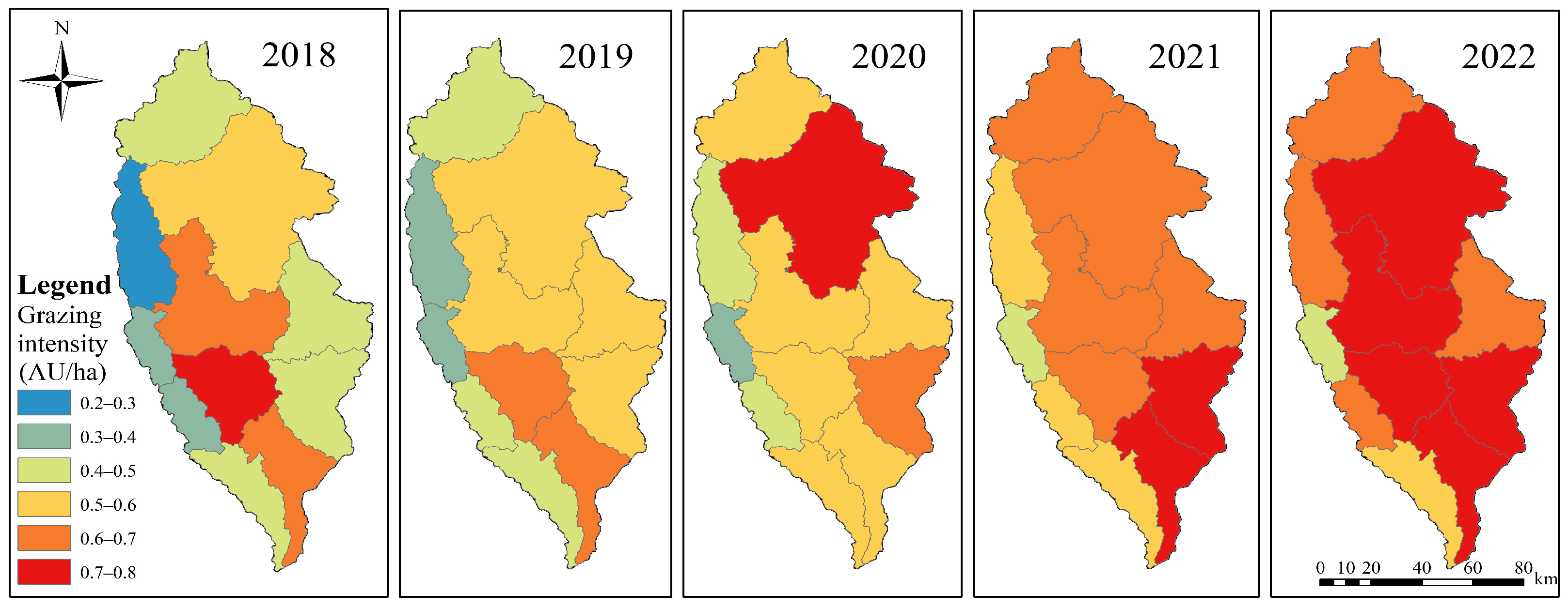
| Year | Number of Grazing Animals (thou) | Growth Rate (%) | Grazing Intensity (AU/ha) | Number of Tourists (thou) | Growth Rate (%) | Tourism Density (Tourists/ha) |
|---|---|---|---|---|---|---|
| 2017 | 249.2 | 10.50 | 0.76 | 15698.3 | 6.00 | 13.52 |
| 2018 | 183.2 | −26.5 | 0.56 | 18147.2 | 15.60 | 15.63 |
| 2019 | 197.2 | 7.64 | 0.60 | 16514.0 | −9.00 | 14.22 |
| 2020 | 210.1 | 6.54 | 0.64 | 6379.0 | −61.37 | 5.49 |
| 2021 | 214.9 | 2.28 | 0.66 | 6724.3 | 5.41 | 5.79 |
| 2022 | 237.1 | 10.33 | 0.73 | 11084.2 | 64.84 | 9.54 |
Disclaimer/Publisher’s Note: The statements, opinions and data contained in all publications are solely those of the individual author(s) and contributor(s) and not of MDPI and/or the editor(s). MDPI and/or the editor(s) disclaim responsibility for any injury to people or property resulting from any ideas, methods, instructions or products referred to in the content. |
© 2025 by the authors. Licensee MDPI, Basel, Switzerland. This article is an open access article distributed under the terms and conditions of the Creative Commons Attribution (CC BY) license (https://creativecommons.org/licenses/by/4.0/).
Share and Cite
Shu, L.; Zhu, Z.; Yin, Y.; Wang, Z.; Wu, W.; Zhang, S.; Liao, S. Impacts of Hydrothermal Factors on the Spatiotemporal Dynamics of Alpine Grassland Aboveground Biomass During the Pre-, Mid-, and Post-COVID-19 Pandemic Periods. Sustainability 2025, 17, 3977. https://doi.org/10.3390/su17093977
Shu L, Zhu Z, Yin Y, Wang Z, Wu W, Zhang S, Liao S. Impacts of Hydrothermal Factors on the Spatiotemporal Dynamics of Alpine Grassland Aboveground Biomass During the Pre-, Mid-, and Post-COVID-19 Pandemic Periods. Sustainability. 2025; 17(9):3977. https://doi.org/10.3390/su17093977
Chicago/Turabian StyleShu, Langlang, Zhening Zhu, Yu Yin, Zizhi Wang, Wengui Wu, Shuqiao Zhang, and Shengxi Liao. 2025. "Impacts of Hydrothermal Factors on the Spatiotemporal Dynamics of Alpine Grassland Aboveground Biomass During the Pre-, Mid-, and Post-COVID-19 Pandemic Periods" Sustainability 17, no. 9: 3977. https://doi.org/10.3390/su17093977
APA StyleShu, L., Zhu, Z., Yin, Y., Wang, Z., Wu, W., Zhang, S., & Liao, S. (2025). Impacts of Hydrothermal Factors on the Spatiotemporal Dynamics of Alpine Grassland Aboveground Biomass During the Pre-, Mid-, and Post-COVID-19 Pandemic Periods. Sustainability, 17(9), 3977. https://doi.org/10.3390/su17093977