Energy Carbon Emission Reduction Based on Spatiotemporal Heterogeneity: A County-Level Empirical Analysis in Guangdong, Fujian, and Zhejiang

Abstract

Guangdong, Fujian, and Zhejiang (GFZ), located on China’s southeast coast, have long been economically active and rapidly growing provinces in China. However, the rising energy consumption in these provinces poses a major challenge to their carbon emissions reduction. Due to the spatial variation in the natural environment and socio-economic activities, energy carbon emissions (ECEs) and their reduction may vary among counties. The matter of scientifically formulating localized carbon reduction paths has therefore become a critical issue. This study proposed a novel path analysis framework based on exploring spatiotemporal heterogeneity using a spatiotemporal statistic model (i.e., spatiotemporal weighted regression). The path’s learning procedure was based on linking the changes in the amount of ECEs to the shifts in dominant factors, which were detected through local significance tests on the coefficients of STWR. To verify its effectiveness, we conducted a county-level empirical study considering four drivers (i.e., population (P), impervious surfaces (I), the proportion of secondary industry (manufacturing, M), and the proportion of tertiary industry (services, S)) in GFZ from 2014 to 2021. The ECEs show two different trends that may be affected by the COVID-19 pandemic and economic recession; hence, we divided them into two periods: an active period (2014–2018) and a stable period (2018–2021). Many interpretable paths and their occurrences were derived from our results, including the following: (1) P and S showed higher sensitivity to the changes in ECEs compared with I and M. Most counties (more than 50%) were dominated by P, but the dominator P may shift to I, M, and S during the active period. Many S-dominated counties reverted to being P-dominated ones during the stable period. (2) For the active period, the two most significant paths, M⁺ → S⁻ and M⁺ → P⁺ (+/− denotes positive or negative impacts of dominated driver), reduced ECEs by about 7.747 × 10⁵ tons and 3.145 × 10⁵ tons, respectively. Meanwhile, the worst path, S⁺ → P⁺, increased ECEs by nearly 1.186 × 10⁶ tons. (3) For the stable period, the best path (S⁺ → I⁺) significantly reduced ECEs by 1.122 × 10⁶ tons, while the worst two paths, M⁻ → P⁺ and I⁺ → P⁺, increased ECEs by 1.978 × 10⁶ tons and 4.107 ×10⁵ tons, respectively. These findings verify the effectiveness of our framework and further highlight the need for tailored, region-specific policies to achieve carbon reduction goals.

1. Introduction

With the rapid growth in the population and the economy, the continuous increase in carbon emissions has exacerbated the “greenhouse effect” [1], leading to frequent extreme climate events such as droughts [2], floods [3], and heat waves [4], which threaten human health and property safety [5]. Since 2007, China has become the world’s largest carbon emitter, accounting for more than 30% of global carbon emissions [6]. To address the international challenges, the Chinese government proposed a “3060 dual carbon” goal (i.e., China will achieve a carbon peak goal by 2030 and a carbon neutrality goal by 2060) [7]. Energy consumption has long played a major role in the growth of carbon emissions. As China’s total energy demand and consumption continue to rise, achieving the goal faces greater challenges [8]. Guangdong, Fujian, and Zhejiang (GFZ), located on the southeast coast of China, have long been the significant economically active and fastest-growing regions in China, and they are facing the contradiction between population growth (increasing energy consumption needs [9]) and poor energy efficiency [10]. The regional reduction in carbon emissions remains a long and arduous road.

In China, there is tension between high consumption [11] and insufficient energy resources [12], and high energy consumption has led to a sharp increase in carbon emissions [13]. Therefore, reducing energy carbon emissions (ECEs) and developing a green low-carbon economy are of far-reaching significance. Path analysis of ECEs reduction can effectively promote the development of low-carbon economies and help formulate policies for accelerating the achievement of the “3060 dual carbon” goals.

Due to the spatial differences in the natural environment and socio-economic activities, pathways toward ECEs reductions may also vary among counties [14]. Estimating the local ECEs is a prerequisite for path analysis. The Intergovernmental Panel on Climate Change (IPCC) provides a general method for accounting for carbon emissions based on energy consumption data [15]. The energy consumption data that can be used to account for ECEs is released by the Energy Statistical Yearbook every year [16]. However, the finest resolution of the published dataset is at the province level rather than the county level, making it impossible to estimate the county-level ECEs.

Thanks to the rapid development of nighttime light (NTL) remote sensing and related technologies, calculating local ECEs based on NTL remote sensing inversion has gradually become a mainstream method [17,18]. Xiang et al. (2024) estimated the county-level ECEs in Jiangsu Province, China, using NPP-VIIRS NTL remote sensing images, and they achieved a relative error of less than 10% [19]. Zheng et al. (2024) used NTL products to estimate energy-related carbon emissions at multiple scales in Fujian Province, including cities, counties, and towns, with an average relative error of −5.27% [20].

Although NTL image inversion has achieved good accuracy in county-level ECEs estimations, research on carbon emission reduction path analysis is still somewhat lagging. There are two main methods used for carbon reduction research: decomposition methods and scenario methods. The former mainly includes the index decomposition analysis (IDA) and structural decomposition analysis (SDA) methods. IDA has two well-known models, i.e., the STIRPAT (stochastic impacts by regression on population, affluence, and technology) model and the LMDI (logarithmic mean Divisia index) model. Although the IDA method can help reveal the compositional structure of carbon emissions, it has some limitations in capturing complex dynamic relationships. For the STIRPAT model, multicollinearity is also prone to occur between different factors [21]. For the LMDI model, it can hardly support in-depth research on more detailed influencing factors [22]. The SDA method can help analyze the impact of economic development and changes in the final demand structure on energy-related carbon emissions. However, this method requires specific data such as input–output and energy balance tables [23]. The scenario methods mainly include the long-range energy alternatives planning system (LEAP) and the system dynamics (SD) model. LEAP can simulate the development paths of various industries in detail but may underestimate the limitations of technology application [24]. Although the SD model can demonstrate the dynamic process of energy consumption and carbon emissions, it has limited adaptability to unforeseen future developments and changes. It is also unable to integrate a variety of dynamic simulation scenarios, which further limits its prediction accuracy [25].

Although these carbon emission reduction analysis methods have achieved positive results, they neglect to explore the dominant role of local driving factors and their transformation relationships from the perspective of temporal and spatial dynamics. Local path analysis of ECEs reduction should consider the major driving factors that affect the ECEs dynamics. Wang et al. (2024) [26] found that population (P) largely contributed to the surge in energy-related carbon emissions in African countries. Zhao et al. (2024) [27] also reported that impervious surface (I), which reflects urbanization, had significantly increased ECEs in China. Su et al. (2018) [28] claimed that the proportion of secondary industry (manufacturing, M) made a significant contribution to the increase in ECEs. Su et al. (2020) found that the increase in the proportion of tertiary industry (services, S) can reduce the ECEs [10]. The above-mentioned factors have direct or indirect impacts on ECEs, but the impacts vary in different regions and periods and require further in-depth analysis.

Exploring the temporal and spatial heterogeneity relationships between local energy carbon emissions and their driving factors is the key to forming the optimal carbon emissions reduction path. Most previous studies analyzed energy carbon emissions reduction and its influencing factors using global modeling methods, such as STIRPAT, LMDI, and others, ignoring the potential local heterogeneity. This limits the formulation of regionally differentiated emission reduction targets and path analysis. Although a set of national-level emission reduction targets has been set in China, adopting the same emission reduction path in different regions may not be conducive to meeting the goal and may even have negative impacts on regional economic development [29]. Therefore, tailoring differentiated targets and optimizing emission reduction paths according to local conditions is critical to ensuring that China achieves its green, low-carbon, and dual goals [30]. Liang et al. (2022) [31] used geographically weighted regression (GWR) to examine the spatial heterogeneity of energy carbon emissions and factors such as urbanization and energy intensity in China. Although this study considered spatial heterogeneity and formulated differentiated carbon emission reduction strategies and recommendations in eastern, central, and western China, temporal heterogeneity may also coexist in real-world processes. To address this issue, Wang et al. (2025) [32] employed geographically and temporally weighted regression (GTWR) to explore the relationships between carbon emissions (CEs) and influencing factors such as the urbanization rate (U) and economic development level (PGDP) and found that the impact of U and PGDP on CE gradually changed from positive to negative, indicating that heterogeneous relationships do change over time. However, the time interval decay weighting strategy adopted by GTWR cannot capture heterogeneity when the rates of value change are inconsistent across locations. This may limit its accuracy in analyzing local spatiotemporal heterogeneity and affect the formation of carbon reduction paths and the reliability of decision support. The spatiotemporal weighted regression (STWR) model [33] adopts a novel decay weighting strategy based on the rate of change of numerical differences, which can better capture local spatiotemporal heterogeneity and has been applied to many studies, such as those of Lyme disease [34], landslides [35], urban heat islands [36,37], etc.

This study aims to develop a path analysis framework based on the STWR model for reducing energy carbon emissions (ECEs) based on their heterogeneous responses to different factors (i.e., P, I, M, and S). It includes the following steps: (1) estimating the county-level ECEs through the inversion of NPP/VIIRS NTL remote sensing images in GFZ regions from 2014 to 2021; (2) generating the spatial coefficient surfaces for P, I, M, and S; and (3) path learning from the significant shifts in dominators and the variations in ECEs.

2. Materials and Methods

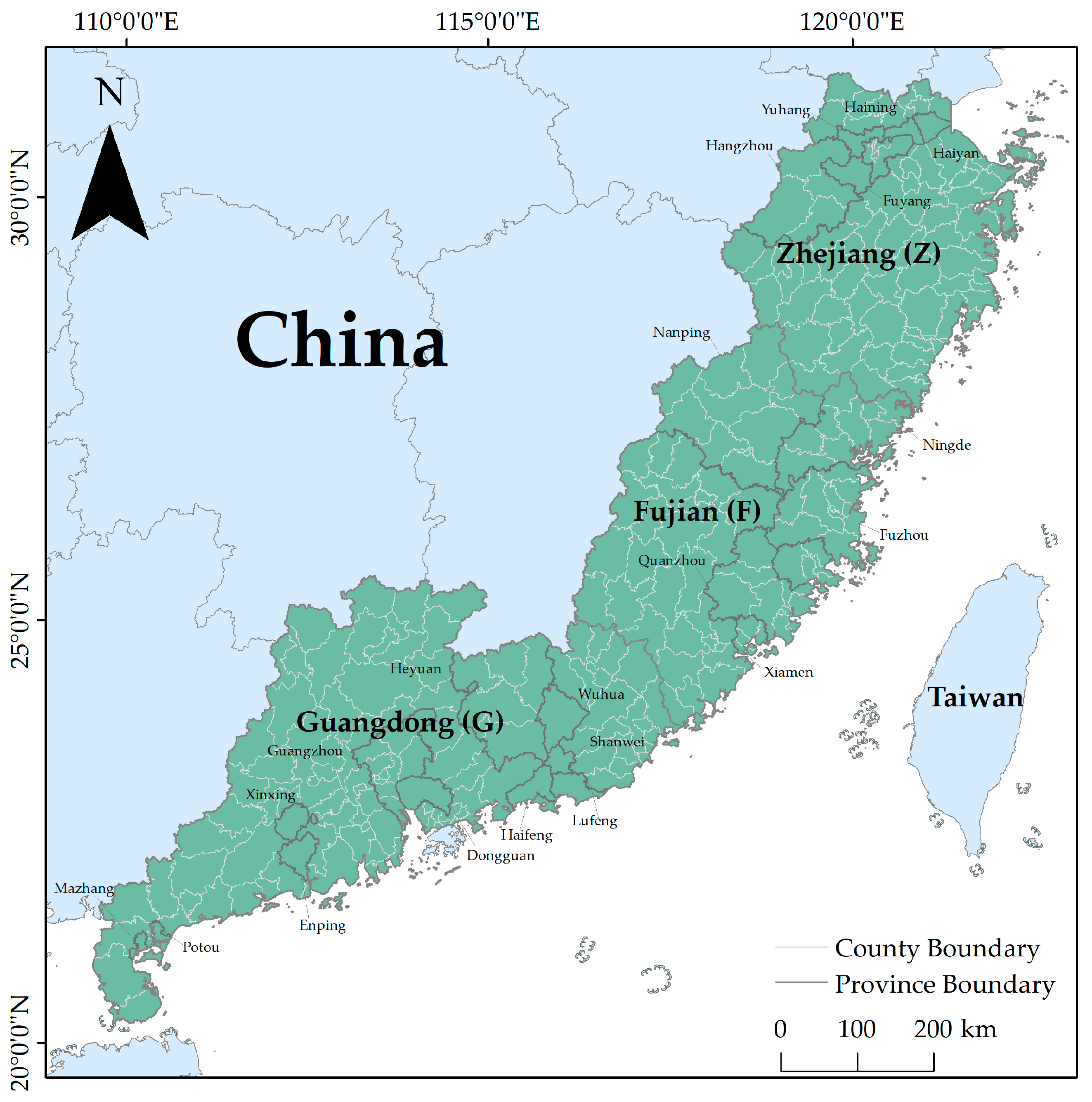
2.1. Study Area and Data Sources

Our study area is the GFZ region (Figure 1), a major engine of China’s economic growth. With a total GDP of CNY 2.1928 trillion, it accounted for around 21.6% of China’s GDP in 2020. However, the total energy consumption of this region also rose from 4.8 billion tons in 2010 to 7.21 billion tons in 2020, which posed a severe challenge to controlling energy consumption and carbon emissions. Many cities in GFZ, such as Xiamen and Hangzhou, are playing pioneering roles in developing China’s low-carbon economy [38]. Exploring the reduction paths of ECEs in GFZ is representative and can be generalized to other post-development regions in China [25,39].

All source data (listed in

Table 1. Data sources.

Data	Source	Resolution
NTL remote sensing images	Earth Observation Group (https://eogdata.mines.edu/products/vnl/, accessed on 30 January 2025)	500 m
Normalized Difference Vegetation Index (NDVI)	Resource and Environmental Science Data Platform (http://www.resdc.cn/, accessed on 30 January 2025)	1000 m
Population (P)	LandScan dataset (https://landscan.ornl.gov/, accessed on 30 January 2025)	1000 m
Proportion of secondary industry (manufacturing, M)	China Economic and Social Big Data Research Platform (https://data.cnki.net/, accessed on 30 January 2025)	County level
Proportion of tertiary industry (services, S)
Impervious surfaces (I)

) were transformed to the WGS_1984_UTM coordinate system and preprocessed using the following steps: (1) Resampling the NTL data to 1000 m, eliminating negative values, and removing outliers according to [40]. (2) Correcting the NTL saturation using Normalized Difference Vegetation Index (NDVI) data according to Equation (2). (3) Cropping the corrected NTL data according to the county boundaries of the GFZ region.

2.2. Methods

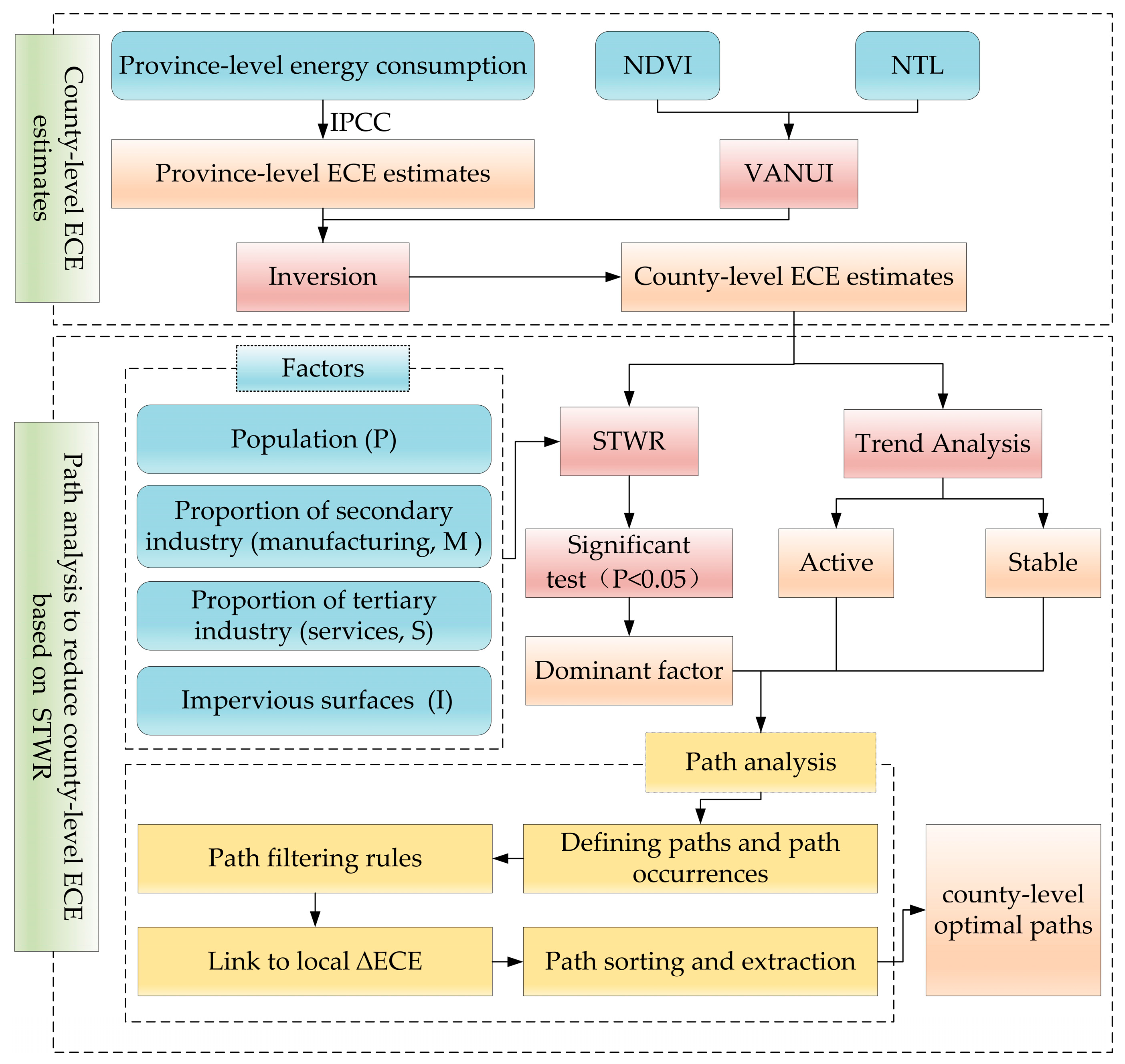
2.2.1. Framework

A path analysis framework for reducing ECEs was designed and proposed (Figure 2), which includes the following steps: (1) Making county-level ECE estimations based on remote sensing image inversion. (2) The significant coefficients generated by STWR were used to detect the shifts in the dominant factors at the county level. (3) Conducting a county-level path analysis based on the links of historical transformations and ECE dynamics.

2.2.2. ECEs Estimates Based on NTL Remote Sensing Inversion

Province-level ECEs can be calculated according to the IPCC using the following equation [15]:

$${\mathrm{E}\mathrm{C}\mathrm{E}}_{\mathrm{I}\mathrm{P}\mathrm{C}\mathrm{C}}=\sum _{\mathrm{n}=1}^{\mathrm{N}}{\mathrm{Q}}_{\mathrm{n}}{\mathrm{C}}_{\mathrm{n}}{\mathrm{F}}_{\mathrm{n}}$$

(1)

where $\mathrm{N}$ and ${\mathrm{Q}}_{\mathrm{n}}$ denote the total number of energy consumption types and the n-th type of energy consumption, respectively. ${\mathrm{C}}_{\mathrm{n}}$ and ${\mathrm{F}}_{\mathrm{n}}$ denote the n-th type of energy consumption’s carbon emission coefficient [41] and standard coal conversion factors [42], respectively.

The NTL saturation may lead to an underestimation of ECEs in highly developed regions, thus causing inaccurate ECE estimates. The Human Settlement Index (HSI) [43], the adjusted nighttime light urban index (VANUI) [44], and the enhanced vegetation index adjusted nighttime light index (EANTLI) [45] are three common methods used to reduce the saturation effect. The HSI uses normalized NTL and the NDVI to eliminate the saturation effect, but when the NDVI approaches zero, its result increases exponentially, resulting in the overcorrection of NTL. The VANUI and EANILI can avoid this issue. In areas with high vegetation coverage, the EVI is considered to have higher sensitivity than the NDVI [46], but the EVI is also more susceptible to terrain undulations [47]. Considering that there are many hills in our study areas of Fujian, Zhejiang, and Guangdong, we use the VANUI method:

$$\mathrm{V}\mathrm{A}\mathrm{N}\mathrm{U}\mathrm{I}=\mathrm{N}\mathrm{T}\mathrm{L}(1-\mathrm{N}\mathrm{D}\mathrm{V}\mathrm{I})$$

(2)

The inversion of ECEs (i.e., ${\mathrm{E}\mathrm{C}\mathrm{E}}_{\mathrm{I}\mathrm{n}\mathrm{v}\mathrm{e}\mathrm{r}\mathrm{s}\mathrm{i}\mathrm{o}\mathrm{n}}$) can be calculated by fitting the provincial-level no-intercept linear regression model, and its formula can be defined as follows [48,49]:

$${\mathrm{E}\mathrm{C}\mathrm{E}}_{\mathrm{I}\mathrm{n}\mathrm{v}\mathrm{e}\mathrm{r}\mathrm{s}\mathrm{i}\mathrm{o}\mathrm{n}}=\mathrm{A}\mathrm{v}\mathrm{e}\left({\displaystyle \frac{{\mathrm{E}\mathrm{C}\mathrm{E}}_{\mathrm{I}\mathrm{P}\mathrm{C}\mathrm{C}}^{\mathrm{P}}}{{\sum }_{\mathrm{m}=1}^{{\mathrm{M}}_{\mathrm{P}}}{\mathrm{V}\mathrm{A}\mathrm{N}\mathrm{U}\mathrm{I}}_{\mathrm{m}}}}\right)\mathrm{V}\mathrm{A}\mathrm{N}\mathrm{U}\mathrm{I}$$

(3)

where ${\mathrm{M}}_{\mathrm{P}}$ denotes the total number of pixels within a given province. ${\mathrm{V}\mathrm{A}\mathrm{N}\mathrm{U}\mathrm{I}}_{\mathrm{m}}$ denotes the $\mathrm{V}\mathrm{A}\mathrm{N}\mathrm{U}\mathrm{I}$ of the m-th pixel. ${\mathrm{E}\mathrm{C}\mathrm{E}}_{\mathrm{I}\mathrm{P}\mathrm{C}\mathrm{C}}^{\mathrm{P}}$ denotes province-level ECEs calculated by Equation (1). $\mathrm{A}\mathrm{v}\mathrm{e}\left(\right)$ is an average function.

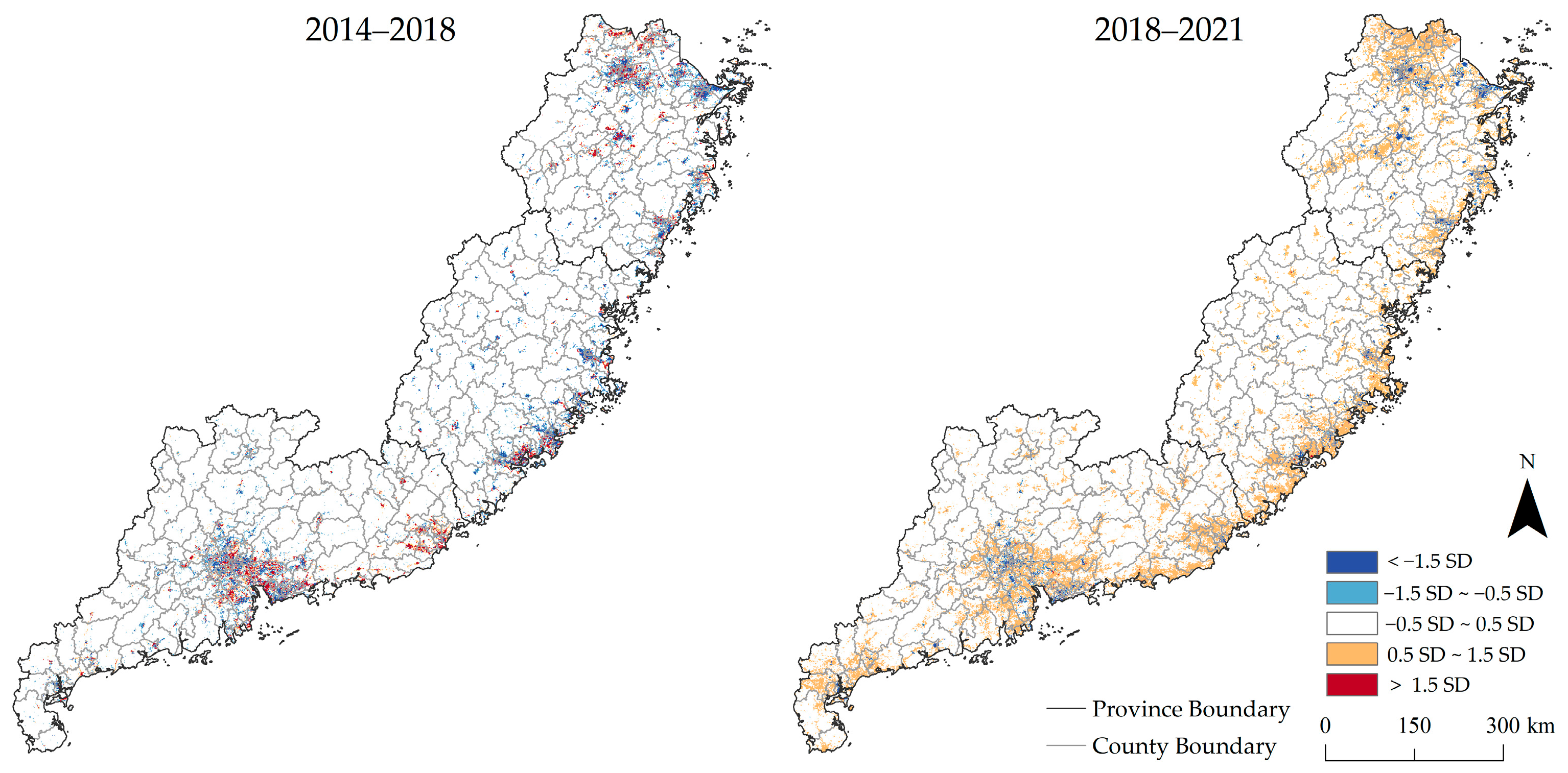
2.2.3. Trend Analysis

We employ a slope function to measure the changing trend in ECEs, and its formula is as follows [18]:

$$\mathrm{S}\mathrm{l}\mathrm{o}\mathrm{p}\mathrm{e}\left(\mathrm{x},\mathrm{t}\right)={\displaystyle \frac{{\mathrm{T}}_{\mathrm{n}}\sum _{\mathrm{t}=1}^{{\mathrm{T}}_{\mathrm{n}}}\mathrm{t}{\mathrm{x}}^{\left(\mathrm{t}\right)}-({\sum }_{\mathrm{t}=1}^{{\mathrm{T}}_{\mathrm{n}}}\mathrm{t}\left)\right({\sum }_{\mathrm{t}=1}^{{\mathrm{T}}_{\mathrm{n}}}{\mathrm{x}}^{\left(\mathrm{t}\right)})}{{\mathrm{T}}_{\mathrm{n}}\sum _{\mathrm{t}=1}^{{\mathrm{T}}_{\mathrm{n}}}{\mathrm{t}}^2-{({\sum }_{\mathrm{t}=1}^{{\mathrm{T}}_{\mathrm{n}}}\mathrm{t})}^2}}$$

(4)

where $\mathrm{x}$ denotes a variable, the trend of which is to be measured. ${\mathrm{x}}^{\left(\mathrm{t}\right)}$ is the value of $\mathrm{x}$ at time $\mathrm{t}$. ${\mathrm{T}}_{\mathrm{n}}$ denotes the total number of $\mathrm{t}$.

2.2.4. STWR

The STWR model employs a decay weighting strategy of time distance (i.e., the numerical difference rate between the observations within a time interval) rather than time interval, which can better explore the local spatiotemporal heterogeneity. Its basic formula is as follows [50]:

$${\mathrm{y}}_{\mathrm{i}}^{\mathrm{t}}={\mathsf{\beta }}_0^{\mathrm{t}}({\mathrm{u}}_{\mathrm{i}},{\mathrm{v}}_{\mathrm{i}})+{\sum }_{\mathrm{k}}{\mathsf{\beta }}_{\mathrm{k}}^{\mathrm{t}}({\mathrm{u}}_{\mathrm{i}},{\mathrm{v}}_{\mathrm{i}}){\mathrm{x}}_{\mathrm{i}\mathrm{k}}^{\mathrm{t}}+{\mathsf{\epsilon }}_{\mathrm{i}}^{\mathrm{t}}$$

(5)

$${\mathsf{\beta }}^{\mathrm{t}}({\mathrm{u}}_{\mathrm{i}},{\mathrm{v}}_{\mathrm{i}})=\left[{\left({\mathrm{X}}_{{\mathrm{O}}_{∆\mathrm{t}}}^{\mathrm{T}}{\mathrm{W}}_{∆\mathrm{t}}\right({\mathrm{u}}_{\mathrm{i}},{\mathrm{v}}_{\mathrm{i}}\left){\mathrm{X}}_{{\mathrm{O}}_{∆\mathrm{t}}}\right)}^{-1}{{\mathrm{X}}_{{\mathrm{O}}_{∆\mathrm{t}}}^{\mathrm{T}}\mathrm{W}}_{∆\mathrm{t}}({\mathrm{u}}_{\mathrm{i}},{\mathrm{v}}_{\mathrm{i}})\right]{\mathrm{y}}_{{\mathrm{O}}_{∆\mathrm{t}}}$$

(6)

where ${\mathrm{y}}_{\mathrm{i}}^{\mathrm{t}}$ and ${\mathrm{x}}_{\mathrm{i}\mathrm{k}}^{\mathrm{t}}$ denote the dependent variable and independent variable of the i-th regression point $({\mathrm{u}}_{\mathrm{i}},{\mathrm{v}}_{\mathrm{i}})$ in period t, respectively. ${\mathsf{\beta }}_{\mathrm{k}}^{\mathrm{t}}({\mathrm{u}}_{\mathrm{i}},{\mathrm{v}}_{\mathrm{i}})$ and ${\mathsf{\epsilon }}_{\mathrm{i}}^{\mathrm{t}}$ denote the regression coefficient and the error term of the i-th regression point in period t, respectively. ${\mathrm{X}}_{{\mathrm{O}}_{∆\mathrm{t}}}$ denotes the matrix of independent variables observed in the time interval $∆\mathrm{t}$. ${\mathrm{W}}_{∆\mathrm{t}}({\mathrm{u}}_{\mathrm{i}},{\mathrm{v}}_{\mathrm{i}})$ denotes the spatiotemporal weight matrix.

Like the GWR model, the STWR model has the following assumptions: (1) There is a local linear relationship between the dependent variable and the independent variables. (2) The random error term has an expected value of zero and follows a normal distribution. (3) The variance is homogeneous and independent of time and space. (4) The different independent variables are independent of each other and the error term. (5) Non-stationarity in space and time: the relationships between variables vary with geographic location and over time rather than being globally stable. (6) Local stationarity: within a certain local spatial range and adjacent time, the relationship between variables remains relatively stable, allowing for parameter estimation through local weighted regression. (7) Neighboring observation points have a greater impact on the current point. The model assigns different weights to observation points at different distances through a weight matrix, reflecting the spatial and temporal attenuation effect.

2.2.5. Steps of Path Analysis

Based on the STWR significance test, we developed a novel path analysis method, which mainly includes the following steps:

(1)

Defining paths and path occurrences. In this study, we regarded the shifts in dominant factors as paths, including their types and the positive and negative impacts (indicated by +/−). Different counties may experience the same path (shift in the dominant factor) at different times, and a single occurrence is a path occurrence corresponding to the path.

(2)

Path filtering rules. To reduce noise and enhance the robustness of the learning path, some rules need to be formulated, such as eliminating paths with fewer occurrences. In this study, we removed paths with less than or equal to 5% of the total path occurrences (the minimum number of occurrences is 4).

(3)

Link to local change in ECEs. Each path occurrence can be linked to a specific county’s ECEs change ($∆\mathrm{E}\mathrm{C}\mathrm{E}$).

(4)

Path sorting and extraction. For each path, we can average all the linked ECEs changes of their path occurrences. Then, we can extract the best path in different counties by sorting or other calculation methods.

3. Results

This study first calculated provincial ECEs for different years, considering seven energy consumption types: coal, coke, gasoline, kerosene, diesel, fuel oil, and natural gas. The carbon emission coefficient and standard coal conversion coefficient corresponding to each energy consumption type refer to the IPCC and the National Energy Administration of China (https://www.nea.gov.cn/, accessed on 30 January 2025).

3.1. Verification of the County-Level ECEs Estimates

To verify the reliability of the ECEs inversion used in this study, we used the IPCC estimation results to verify our inversion results, and the results are shown in

Table 2. Relative error (RE) (%).

Area	Average	2014	2015	2016	2017	2018	2019	2020	2021
Guangdong	12.29	−11.45	−14.51	−20.27	−15.05	1.43	2.36	13.94	19.27
Fujian	7.91	−17.75	−13.12	−8.19	7.16	2.74	1.12	5.85	7.32
Zhejiang	13.02	22.75	22.90	15.00	3.40	1.35	−9.32	−13.15	−16.29

. The average relative errors of Guangdong, Fujian, and Zhejiang are 12.29%, 7.91%, and 13.03%, respectively. In addition, we collected public data (city level) for Fuzhou in 2020 and 2021 (https://tjj.fuzhou.gov.cn/zzbz/tjxx/tjnj/, accessed on 30 January 2025) and verified using the IPCC method that the RE values of our inversion results were 8.8% and 1.5%, respectively (data from other years are incomplete and therefore cannot be compared).

3.2. Analysis of ECEs Trends

We calculated pixel-level slopes using Equation (4) and found there existed two different trends. Considering that the two trends may be caused by the COVID-19 pandemic, they may reflect two different stages or modes of economic development. Other studies [51,52] also reported that the COVID-19 pandemic not only significantly affected the energy demand but also caused economic recessions in many regions after 2019. Therefore, by distinguishing these two periods, we should be able to conduct a more in-depth analysis of the carbon emissions reduction paths under different trends, thereby providing decision-makers with more effective carbon emissions reduction policy analysis results. Therefore, we divided the data into two periods: active (2014–2018) and stable (2018–2021) (the 2018 ECEs data were used in both periods, mainly to compare and examine the differences in slopes before and after 2018). For the former period, the mean and standard deviation (SD) of the ECEs’ slopes are 0.014 and 0.054, respectively. For the latter period, the mean and SD of its slopes are −0.0145 and 0.037, respectively. To illustrate the differences, we categorized the slopes into five groups (

Table 3. Slope estimates of ECEs.

Groups	Activate Period (2014–2018)	Stable Period (2018–2021)
<−1.5 SD	Slope < −0.067	Slope < −0.070
−1.5 SD~−0.5 SD	−0.067 ≤ Slope < −0.013	−0.070 ≤ Slope < −0.033
−0.5 SD~0.5 SD	−0.013 ≤ Slope < 0.041	−0.033 ≤ Slope < 0.004
0.5 SD~1.5 SD	0.041 ≤ Slope < 0.095	0.004 ≤ Slope < 0.041
≥1.5 SD	Slope ≥ 0.095	Slope ≥ 0.041

Note: SD denotes the standard deviation.

): “<−1.5 SD” (i.e., less than mean −1.5 SD), “−1.5 SD~−0.5 SD” (i.e., ranges between mean − 1.5 SD and mean − 0.5 SD), “−0.5 SD~0.5 SD” (i.e., ranges between mean − 0.5 SD and mean + 0.5 SD), “0.5 SD~1.5 SD” (i.e., ranges between mean + 0.5 SD and mean + 1.5 SD), and “>1.5 SD” (i.e., greater than mean + 1.5 SD). As shown in Figure 3, the absolute standard deviations of the ECE’s slopes in many counties during the active period are significantly different from the mean, while they are relatively closer to the mean during the stable period.

3.3. Spatiotemporal Heterogeneity

3.3.1. Multicollinearity Diagnostics

To avoid multicollinearity, we conducted multicollinearity diagnostics on the factors P, I, M, and S. As shown in

Table 4. Results of multicollinearity diagnostics.

	P	I	M	S
VIF	1.128	1.891	3.484	4.612
Tolerance	0.886	0.529	0.287	0.217

, all the variance inflation factors (VIFs) were less than 5, and the collinearity tolerance (Tolerance) values were all less than 1 and greater than 0.1, indicating that there was no obvious collinearity.

We compared the results of the OLS, GWR, and STWR models from 2014 to 2021. As shown in

Table 5. Comparison of model performance of OLS, GWR, and STWR.

Year	Model	R2	AICc	SSE
2014	OLS	0.775	412.289	67.177
	GWR	0.926	248.566	22.235
	STWR	0.936	260.196	19.090
2015	OLS	0.779	407.101	66.021
	GWR	0.927	240.822	21.720
	STWR	0.957	61.409	12.777
2016	OLS	0.788	395.476	63.504
	GWR	0.928	239.112	21.555
	STWR	0.997	−606.769	0.874
2017	OLS	0.802	375.143	59.329
	GWR	0.942	189.133	17.402
	STWR	0.994	−388.742	1.684
2018	OLS	0.799	378.736	60.046
	GWR	0.934	211.395	19.689
	STWR	0.998	−549.380	0.490
2019	OLS	0.816	353.139	55.120
	GWR	0.936	214.841	19.262
	STWR	0.998	−398.609	0.670
2020	OLS	0.822	343.044	53.290
	GWR	0.942	181.151	17.223
	STWR	0.997	−531.810	0.927
2021	OLS	0.819	347.381	54.068
	GWR	0.938	201.057	18.575
	STWR	0.997	−574.186	0.921

, all the results of STWR models have the best R-squared (R²), sum of square error (SSE), and Akaike information criterion correction (AICc).

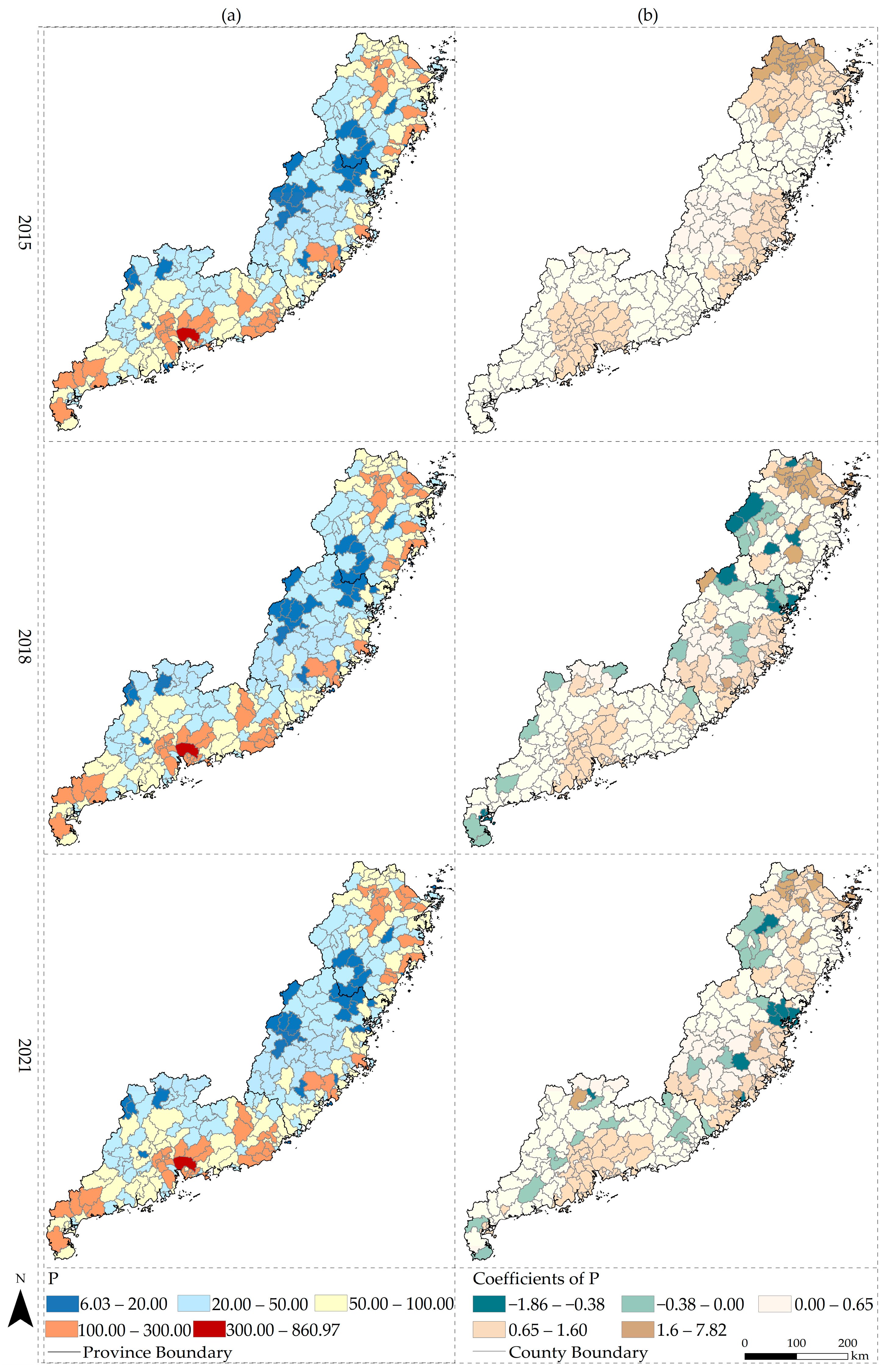
3.3.2. Impacts of Population (P)

Figure 4 shows the spatial distribution of P and its corresponding coefficients, indicating that P positively impacts ECEs in most counties, especially surrounding some major cities, such as Guangzhou, Hangzhou, and Fuzhou, etc. Meanwhile, the scope and extent of the impact show a shrinking trend. The coefficients of counties close to the boundary of Fujian and Zhejiang showed negative results, indicating that the increase in population may, to a certain extent, reduce ECEs in some regions with low population density.

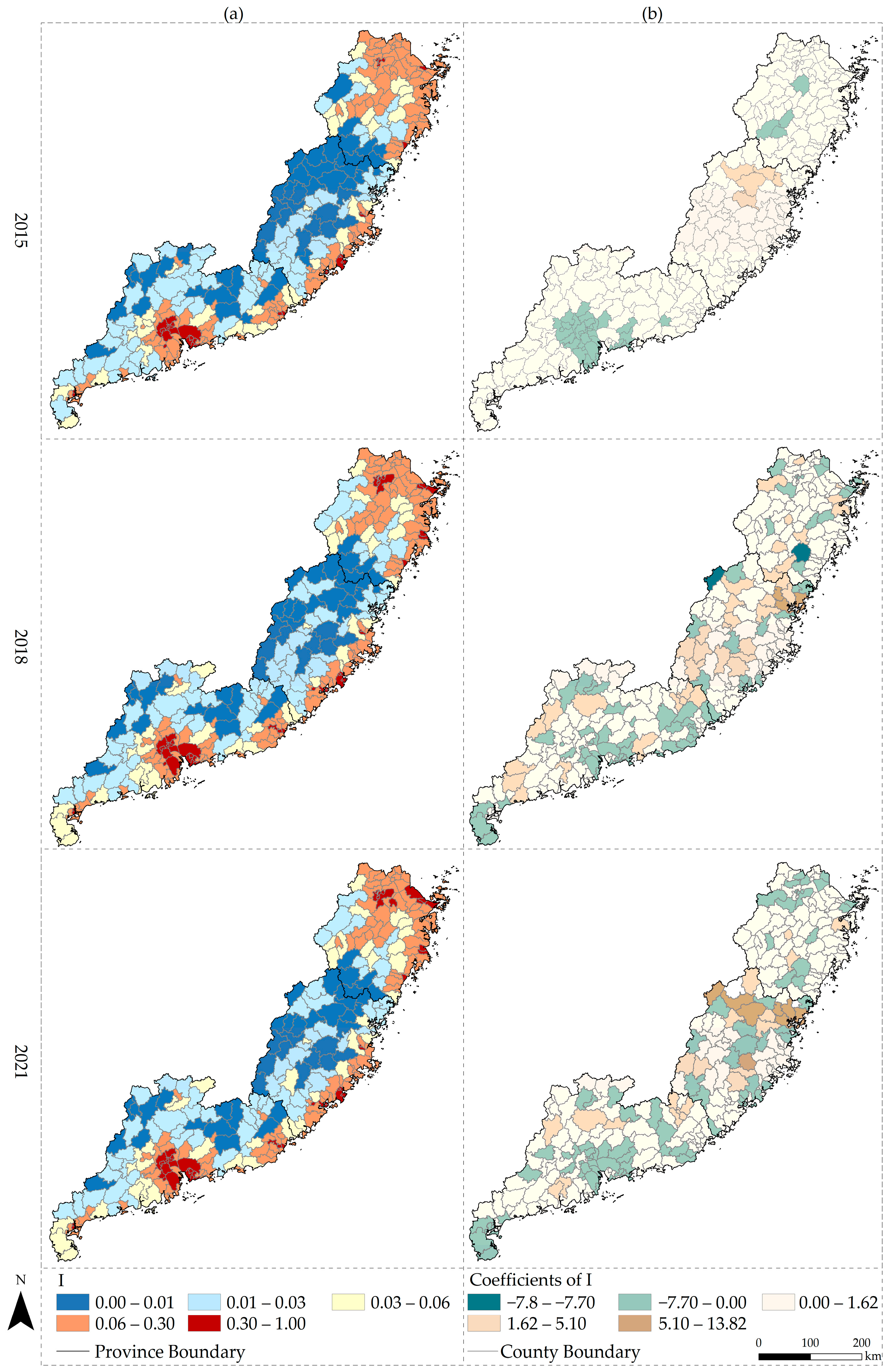
3.3.3. Impacts of Impervious Surfaces (I)

Figure 5 shows the spatial distribution of I and its corresponding coefficients. For counties with lower urbanization levels (such as Nanping and Ningde), the positive impact of I continues to increase; for counties with higher urbanization levels (such as Quanzhou and Hangzhou), it shows a clear negative effect. These results are consistent with those in [53], which may be interpreted as meaning that the increase in impervious surface areas in the early stages of urbanization has a significant positive impact on the increase in ECEs, while, in the later stages of urbanization, the impact of impervious surfaces decreases.

3.3.4. Impacts of Manufacturing (M)

Figure 6 shows the spatial distribution of M and its corresponding coefficients. There are significant negative impacts on counties with strong manufacturing industries (such as Dongguan and Haiyan), which may be related to the lower carbon emission intensity per unit of output value.

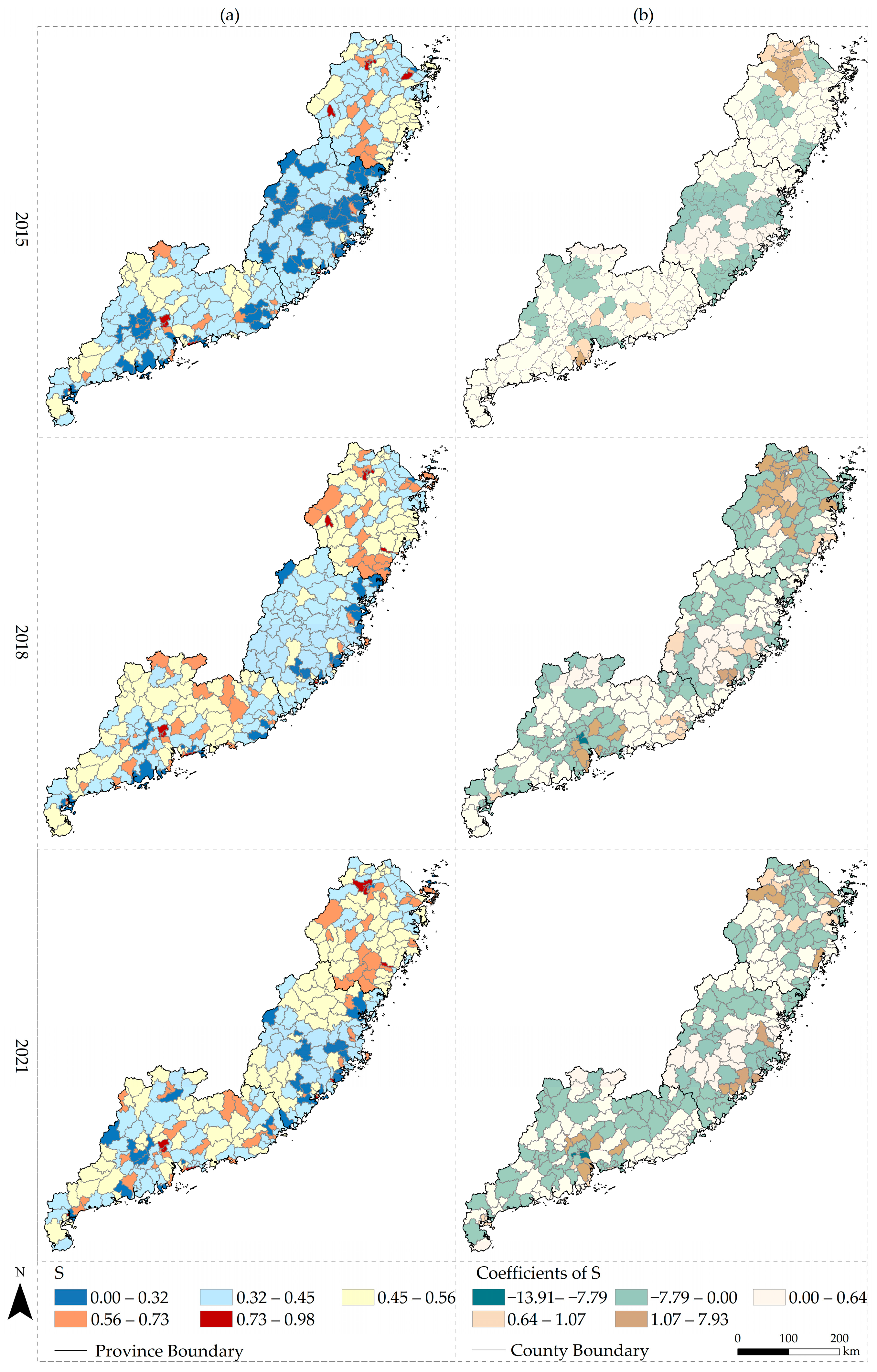
3.3.5. Impacts of Services (S)

Figure 7 shows the spatial distribution of S and its corresponding coefficient, indicating that most counties have a negative impact on ECEs, and the scope and degree of their impact tend to expand. Some positive effects appeared in some counties in northern Zhejiang (such as Fuyang and Yuhang), which may indicate that the large-scale growth of S may still promote ECEs, to a certain extent [54].

3.4. Path Analysis

To obtain more reliable path analysis results, we conducted a significance test of α = 0.05 on each coefficient surface generated by STWR and plotted the leading factors of counties that passed the test in different periods on the map. Based on the transformation of dominant factors and the change in ECEs, we conducted path learning and analysis. As shown in Figure 8, P was the dominator for most counties (about 50.58% on average), followed by I, which is consistent with [55]. P and S showed higher sensitivity to the changes in ECEs compared with I and M. The number of P-dominant counties first decreased from 180 in 2015 to 102 in 2018, and then slightly increased to 109 in 2021. During the active period (2015–2018), most P-dominant counties shifted to I-, M-, and S-dominant ones, especially the counties in Fujian and Zhejiang. However, during the stable period (2018–2021), many of the S-dominant counties reverted to being S-dominant ones. The number of I- and M-dominant counties remained relatively stable. These shifts may relate to the decline in service activities [56] and the slowdown in urbanization [57] caused by the COVID-19 pandemic.

Figure 9 shows the results of county-level paths learned from our framework associated with their average change in ECEs during the active and stable periods. For the active period, the path “S⁺ → P⁺” was the most significantly related to ECEs, contributing about 1.119 × 10⁶ tons of carbon emissions. This path mainly occurred in counties such as Heyuan and Shanwei, indicating that these counties were facing severe carbon emission reduction situations. The path “M⁺ → S⁻” was recommended for it minimized ECEs by about 7.747 × 10⁵ tons. For the stable period, path “S⁺ → I⁺” is recommended because it reduced the amount of ECEs by about 1.122 ×10⁶. The “M⁻ → P⁺” path is the worst, because it stimulated the growth of ECEs, with an increase of about 1.978 ×10⁶ tons. This may be because of the decline in manufacturing caused by COVID-19 [58]. The “I⁺ → P⁺” path is the second worst because it increased the ECEs by about 4.107 ×10⁵ tons, which indicated that the slowdown of urbanization may not necessarily reduce ECEs.

For most counties that are currently dominated by the factor P⁺, “ P⁺ → M⁻” would be a wise choice because it reduced ECEs by about 1.765 × 10⁵ tons and 1.28 × 10⁴ tons in the active and stable periods, respectively. This path indicates that improving the quality of manufacturing and migrating the population from industries with high per capita carbon emissions to high-tech manufacturing may be beneficial for reducing ECEs.

4. Discussion

This study proposed a novel path analysis framework for carbon emissions reduction based on spatiotemporal heterogeneity. The STWR model was employed to explore the spatiotemporal heterogeneity and to detect the local dominant factors. Path learning supported by the framework can be conducted by binding the historical shifts in dominant factors and the change in the amount of local ECEs. Several interesting findings were detected in our county-level empirical study, which preliminarily verified the effectiveness of this framework.

(1)

It supports the dynamic path analysis of local carbon reduction. Most path analyses for reducing carbon emissions are based on global models, meaning that they ignore the local variations in relationships in space and time. The proposed framework incorporated spatiotemporal heterogeneity using the STWR model and established a channel for path learning, i.e., learning from binding the shifts in dominant factors and the change in the amount of carbon emissions. Therefore, it provides sophisticated, map-based visual support for forming regionally and temporally differentiated carbon reduction paths.

(2)

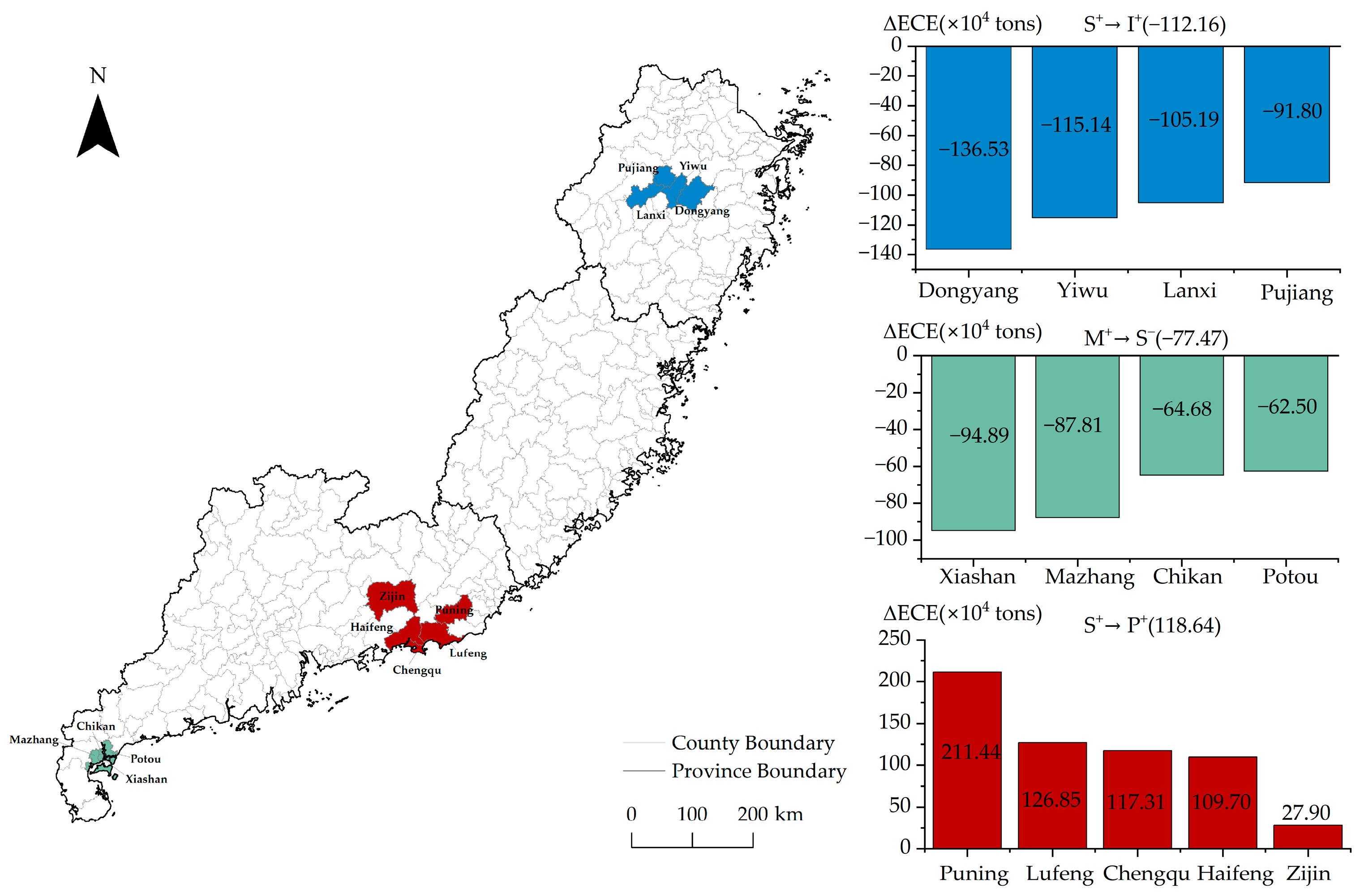
The learned path from the framework is a strong indicative reference because it is tied to carbon emissions; it is therefore able to indicate the amount of increase or decrease in carbon emissions. The local dominant factor is detectable, so the local optimal path and expected carbon emission changes under different development periods (modes) can be predicted and mapped. Supposing that a county’s current dominant factor is “M+”, if the current ECEs are during the active period, the “M+ → S−” path would be preferred because it reduced about 7.747 × 105 tons of ECEs in the past. During the stable period, the path “M+ → P+” would be better because it increased the ECEs the least, by about 1.112 × 105 tons. The practical guiding significance of these two paths is also very strong. For fast-growing regions, the former path can be pursued to reduce carbon emissions and achieve high-quality growth, while, for slower-growing regions, the latter path may be more suitable to control carbon emission growth. Figure 9c,f show the optimal paths for reducing ECEs at the county level for the active and stable periods, respectively.

(3)

Each path learned from the framework can be tracked for its corresponding shift occurrences, including occurrence times and locations. This feature can provide references for regions with similar development patterns and is conducive to analyzing regional abnormal carbon emissions. Many paths detected in our empirical analysis are highly interpretable. Figure 10 shows three paths, “S+ → I+”, “M+ → S−”, and “S+ → P+”, and all their corresponding counties and related amounts of ECEs. Counties with the same path show clustering characteristics in space. “S+ → I+” occurred in four counties: Dongyang, Yiwu, Lanxi, and Pujiang. The reductions made by this path are significant and relatively uniform. This result may be related to the effectiveness of these counties in actively promoting the construction of smart cities, which is consistent with [59]. “M+ → S−” occurred in four counties: Xiashan, Mazhang, Chikan, and Potou. The average proportion of these counties’ secondary and tertiary industries (M and S) changed from 50.4% and 43.6% in 2015 to 47.95% and 46.83% in 2018. The service industry (S), which has low energy consumption and high added value, has gradually increased, reducing ECEs. “S+ → P+” occurred in five counties: Puning, Lufeng, Chengqu, Haifeng, and Zijin. The increased amount of ECEs may be caused by the loss of the high-tech population and the improvement in the service quality of S (the tertiary industry) in these counties. That is, these counties may have an insufficient proportion of people engaged in high-tech (low-carbon emission) industries, while a large proportion of people are engaged in low-end industries with high carbon emissions, which has led to a surge in ECEs. It is worth noting that although the overall change in the amounts of carbon emissions fluctuates around the average, some individual counties have large deviations. If more data are used, the number of occurrences of each path increases, making it more stable and reliable.

(4)

This study also supports a comparative analysis of the selected counties and of counties with similar conditions. As shown in

Table 6. Comparison of path occurrence and related information.

Area	Path	$∆\mathbf{E}\mathbf{C}\mathbf{E}$$(\times {10}^4$ Tons)	$∆\mathbf{P}$ (%)	$∆\mathbf{M}$ (%)	$∆\mathbf{S}$
Enping	P+ → I+	137.0 → 157.4 (20.4)	515,765 → 525,587 (1.9%)	29.9% → 27.6% (−7.7%)	59.7% → 56.8% (−4.9%)
Xinxing	P+ → I+	115.1 → 148.7 (33.6)	447,996 → 452,660 (1.0%)	30.3% → 34.8% (14.9%)	48.1% → 40.6% (−15.6%)
Lufeng	P+ → P+	345.0 → 465.7(120.7)	1,407,137 → 1,415,325 (0.1%)	42.9% → 40.6% (−5.4%)	37.0% → 40.8% (10.3%)

, Enping and Xinxing counties are very close in terms of spatial location (Figure 1), ECEs, dominant factors, population, industrial structure, etc. Their ECEs values are both around 1.5 million tons, with a difference of less than 500,000 tons. Their populations are both around 470,000. Their proportions of secondary industry (manufacturing, M) are about 30%, less than their proportion of tertiary industry (service, S). Their dominant factors have shifted from P+ to I+. However, the conditions of Lufeng County are quite different from those of Enping and Xinxing. Its ECEs exceeded 3 million tons, with a change of more than 1 million tons. Its population doubled to 1.4 million. S was higher than M, and its dominant factor remained unchanged.

(5)

By conducting an empirical analysis, we can form “tailor-made” countermeasures for different regions. On the one hand, different counties should adopt different countermeasures. For counties with lower S values, such as Mazhang and Potou, “M+ → S−” is the most effective path (Figure 9b). For areas with higher S values, such as Dongyang and Yiwu, “S+ → I+” is the most effective path (Figure 9e). Therefore, for counties such as Mazhang and Potou, the development of tertiary industry (S) should be actively promoted in the future. In terms of tax incentives, reduction and exemption can be increased according to the progress of enterprise transformation; for Dongyang and Yiwu, the construction of smart cities could be accelerated, and the corresponding supporting infrastructure can be established. On the other hand, for the same county, different countermeasures should be taken according to different development stages (at different times). For example, for counties with low populations, such as Xiashan and Chikan, the path “M+ → S−” significantly reduced energy carbon emissions during the active period (Figure 9b), while, in the stable period, the path “S− → P+” (Figure 9e) effectively reduced energy carbon emissions. Therefore, during the active period, we can increase support for tertiary industry (S) and promote the transformation of secondary industry (M) to tertiary industry (S). During the stable period, we can strengthen talent policies, such as by providing housing subsidies and preferential treatment for children’s schooling, to attract high-tech talents.

Although the proposed framework and its empirical analysis have yielded some results, it still has many limitations. Some of those that need further consideration are listed below:

(1)

Although the locally optimal path and its related amount of carbon emissions can be learned from our framework, the matter of how to guide the achievement of the optimal path remains unknown. Some optimal paths (i.e., shifts in dominant factors) learned from other regions may also face significant challenges when implemented locally. Therefore, further research is needed to more specifically guide regions to complete the transition to the optimal paths.

(2)

Due to some limitations in data availability, our empirical analysis only considered four factors (i.e., P, I, M, and S), but there may be many other factors that affect regional ECEs in the real world. Further study can consider more socio-economic factors, such as the import and export trade volume, scientific and technological research and development investment, the number of high-tech enterprises, etc. Moreover, a broader carbon reductions (not just ECEs) study should be considered.

(3)

The estimation of local ECEs based on NTL remote sensing image inversion may have different errors in space and time. The reasons for these errors may be multifaceted. Although the VANUI method used in this study can effectively reduce the saturation effect of NTL to a certain extent, for areas with large NDVI values, the VANUI will not increase the variability in NTL values in the region [44]. The NDVI data obtained by satellite remote sensing will also be affected by factors such as atmospheric interference and cloud cover, resulting in errors [60]. This, in turn, will affect the final ECEs estimation. Subsequent research may consider using a more scientific remote sensing image inversion model.

(4)

The adopted STWR model has the following main limitations, which may affect the reliability of the analysis results: (1) The model has only one (initial) spatial and one temporal bandwidth and does not support multi-scale analysis. (2) There is still room for improvement in the local spatiotemporal weight configuration and parameter optimization calibration process. (3) The model assumes a locally linear relationship, but the real-world situation may be non-linear and more complicated.

5. Conclusions

In the face of increasingly frequent extreme climate events, reducing carbon emissions has become a consensus among many people around the world. The extraction and analysis of regionally and temporally differentiated carbon emissions reduction paths is a topic worthy of in-depth discussion. This study focuses on the establishment of a path analysis framework for reducing energy carbon emissions (ECEs) from the perspective of local spatiotemporal heterogeneity. We proposed an STWR-based framework that ties the amount of carbon emissions to the local shifts in dominant factors. A county-level empirical study on the energy carbon emissions of the GFZ (Guangdong, Fujian, and Zhejiang) provinces preliminarily verified its effectiveness. The paths learned from the framework can also be tracked in detailed path occurrences including their times and locations, which can facilitate deep interpretation and analysis. This framework is also flexible and may even be transformed into a basic framework for some other resource-saving path analysis.

References

- Ledley, T.S.; Sundquist, E.T.; Schwartz, S.E.; Hall, D.K.; Fellows, J.D.; Killeen, T.L. Climate change and greenhouse gases. Eos Trans. Am. Geophys. Union 1999, 80, 453–458. [Google Scholar]
- Mora, C.; Spirandelli, D.; Franklin, E.C.; Lynham, J.; Kantar, M.B.; Miles, W.; Smith, C.Z.; Freel, K.; Moy, J.; Louis, L.V. Broad threat to humanity from cumulative climate hazards intensified by greenhouse gas emissions. Nat. Clim. Chang. 2018, 8, 1062–1071. [Google Scholar]
- Mitchell, J.F.; Lowe, J.; Wood, R.A.; Vellinga, M. Extreme events due to human-induced climate change. Philos. Trans. R. Soc. A Math. Phys. Eng. Sci. 2006, 364, 2117–2133. [Google Scholar]
- Gasparrini, A.; Guo, Y.; Sera, F.; Vicedo-Cabrera, A.M.; Huber, V.; Tong, S.; Coelho, M.d.S.Z.S.; Saldiva, P.H.N.; Lavigne, E.; Correa, P.M. Projections of temperature-related excess mortality under climate change scenarios. Lancet Planet. Health 2017, 1, e360–e367. [Google Scholar] [PubMed]
- Gillett, N.P.; Shiogama, H.; Funke, B.; Hegerl, G.; Knutti, R.; Matthes, K.; Santer, B.D.; Stone, D.; Tebaldi, C. The Detection and Attribution Model Intercomparison Project (DAMIP v1.0) contribution to CMIP6. Geosci. Model Dev. 2016, 9, 3685–3697. [Google Scholar]
- Li, X.; Lin, C.; Lin, M.; Jim, C.Y. Drivers, scenario prediction and policy simulation of the carbon emission system in Fujian Province (China). J. Clean. Prod. 2024, 434, 140375. [Google Scholar] [CrossRef]
- Yang, P.; Peng, S.; Benani, N.; Dong, L.; Li, X.; Liu, R.; Mao, G. An integrated evaluation on China’s provincial carbon peak and carbon neutrality. J. Clean. Prod. 2022, 377, 134497. [Google Scholar]
- Bai, Y.; Zhou, P.; Tian, L.; Meng, F. Desirable strategic petroleum reserves policies in response to supply uncertainty: A stochastic analysis. Appl. Energy 2016, 162, 1523–1529. [Google Scholar] [CrossRef]
- Wang, C.; Wang, F.; Zhang, X.; Deng, H. Analysis of influence mechanism of energy-related carbon emissions in Guangdong: Evidence from regional China based on the input-output and structural decomposition analysis. Environ. Sci. Pollut. Res. 2017, 24, 25190–25203. [Google Scholar] [CrossRef]
- Su, K.; Wei, D.; Lin, W. Influencing factors and spatial patterns of energy-related carbon emissions at the city-scale in Fujian province, Southeastern China. J. Clean. Prod. 2020, 244, 118840. [Google Scholar]
- Yang, L.; Wang, J.; Shi, J. Can China meet its 2020 economic growth and carbon emissions reduction targets? J. Clean. Prod. 2017, 142, 993–1001. [Google Scholar]
- Li, N.; Zhang, X.; Shi, M.; Zhou, S. The prospects of China’s long-term economic development and CO2 emissions under fossil fuel supply constraints. Resour. Conserv. Recycl. 2017, 121, 11–22. [Google Scholar]
- Abbasi, K.R.; Shahbaz, M.; Zhang, J.; Irfan, M.; Alvarado, R. Analyze the environmental sustainability factors of China: The role of fossil fuel energy and renewable energy. Renew. Energy 2022, 187, 390–402. [Google Scholar]
- Fang, K.; Tang, Y.; Zhang, Q.; Song, J.; Wen, Q.; Sun, H.; Ji, C.; Xu, A. Will China peak its energy-related carbon emissions by 2030? Lessons from 30 Chinese provinces. Appl. Energy 2019, 255, 113852. [Google Scholar]
- Eggleston, H.; Buendia, L.; Miwa, K.; Ngara, T.; Tanabe, K. 2006 IPCC Guidelines for National Greenhouse Gas Inventories; IGES: Hayama, Japan, 2006. [Google Scholar]
- Chen, J.; Gao, M.; Huang, S.; Hou, W. Application of remote sensing satellite data for carbon emissions reduction. J. Chin. Econ. Bus. Stud. 2021, 19, 109–117. [Google Scholar]
- Liu, X.; Ou, J.; Wang, S.; Li, X.; Yan, Y.; Jiao, L.; Liu, Y. Estimating spatiotemporal variations of city-level energy-related CO2 emissions: An improved disaggregating model based on vegetation adjusted nighttime light data. J. Clean. Prod. 2018, 177, 101–114. [Google Scholar]
- Zhang, Z.; Fu, S.; Li, J.; Qiu, Y.; Shi, Z.; Sun, Y. Spatiotemporal Analysis and Prediction of Carbon Emissions from Energy Consumption in China through Nighttime Light Remote Sensing. Remote Sens. 2023, 16, 23. [Google Scholar] [CrossRef]
- Xiang, C.; Mei, Y.; Liang, A. Analysis of Spatiotemporal Changes in Energy Consumption Carbon Emissions at District and County Levels Based on Nighttime Light Data—A Case Study of Jiangsu Province in China. Remote Sens. 2024, 16, 3514. [Google Scholar] [CrossRef]
- Zheng, Y.; Fan, M.; Cai, Y.; Fu, M.; Yang, K.; Wei, C. Spatio-temporal pattern evolution of carbon emissions at the city-county-town scale in Fujian Province based on DMSP/OLS and NPP/VIIRS nighttime light data. J. Clean. Prod. 2024, 442, 140958. [Google Scholar]
- Li, W.; Gao, S. Prospective on energy related carbon emissions peak integrating optimized intelligent algorithm with dry process technique application for China’s cement industry. Energy 2018, 165, 33–54. [Google Scholar] [CrossRef]
- Wang, P.; Wu, W.; Zhu, B.; Wei, Y. Examining the impact factors of energy-related CO2 emissions using the STIRPAT model in Guangdong Province, China. Appl. Energy 2013, 106, 65–71. [Google Scholar] [CrossRef]
- Chong, C.H.; Tan, W.X.; Ting, Z.J.; Liu, P.; Ma, L.; Li, Z.; Ni, W. The driving factors of energy-related CO2 emission growth in Malaysia: The LMDI decomposition method based on energy allocation analysis. Renew. Sustain. Energy Rev. 2019, 115, 109356. [Google Scholar] [CrossRef]
- Huang, R.; Zhang, S.; Wang, P. Key areas and pathways for carbon emissions reduction in Beijing for the “Dual Carbon” targets. Energy Policy 2022, 164, 112873. [Google Scholar] [CrossRef]
- Lin, C.; Li, X. Carbon peak prediction and emission reduction pathways exploration for provincial residential buildings: Evidence from Fujian Province. Sustain. Cities Soc. 2024, 102, 105239. [Google Scholar] [CrossRef]
- Wang, J.; Shan, Y.; Cui, C.; Zhao, C.; Meng, J.; Wang, S. Investigating the fast energy-related carbon emissions growth in African countries and its drivers. Appl. Energy 2024, 357, 122494. [Google Scholar] [CrossRef]
- Zhao, J.; Chen, W.; Liu, Z.; Liu, W.; Li, K.; Zhang, B.; Zhang, Y.; Yu, L.; Sakai, T. Urban expansion, economic development, and carbon emissions: Trends, patterns, and decoupling in mainland China’s provincial capitals (1985–2020). Ecol. Indic. 2024, 169, 112777. [Google Scholar] [CrossRef]
- Su, W.; Liu, Y.; Wang, S.; Zhao, Y.; Su, Y.; Li, S. Regional inequality, spatial spillover effects, and the factors influencing city-level energy-related carbon emissions in China. J. Geogr. Sci. 2018, 28, 495–513. [Google Scholar] [CrossRef]
- Wang, Y.; Yang, H.; Sun, R. Effectiveness of China’s provincial industrial carbon emission reduction and optimization of carbon emission reduction paths in “lagging regions”: Efficiency-cost analysis. J. Environ. Manag. 2020, 275, 111221. [Google Scholar] [CrossRef]
- Wang, J.; Lv, K.; Bian, Y.; Cheng, Y. Energy efficiency and marginal carbon dioxide emission abatement cost in urban China. Energy Policy 2017, 105, 246–255. [Google Scholar] [CrossRef]
- Liang, X.; Min, F.; Xiao, Y.; Yao, J. Temporal-spatial characteristics of energy-based carbon dioxide emissions and driving factors during 2004–2019, China. Energy 2022, 261, 124965. [Google Scholar] [CrossRef]
- Wang, N.; Qu, Z.; Li, J.; Zhang, Y.; Wang, H.; Xi, H.; Gu, Z. Spatial-temporal patterns and influencing factors of carbon emissions in different regions of China. Environ. Res. 2025, 276, 121447. [Google Scholar] [PubMed]
- Que, X.; Ma, X.; Ma, C.; Chen, Q. A Spatiotemporal Weighted Regression Model (STWRv1. 0) for Analyzing Local Non-stationarity in Space and Time. Geosci. Model Dev. Discuss. 2020, 2020, 6149–6164. [Google Scholar] [CrossRef]
- Wang, Z.; Que, X.; Li, M.; Liu, Z.; Shi, X.; Ma, X.; Fan, C.; Lin, Y. Spatiotemporally weighted regression (STWR) for assessing Lyme disease and landscape fragmentation dynamics in Connecticut towns. Ecol. Inform. 2024, 84, 102870. [Google Scholar]
- Que, X.; Zhuang, X.; Ma, X.; Lai, Y.; Xie, J.; Fei, T.; Wang, H.; Yuming, W. Modeling the spatiotemporal heterogeneity and changes of slope stability in rainfall-induced landslide areas. Earth Sci. Inform. 2024, 17, 51–61. [Google Scholar] [CrossRef]
- Fan, C.; Que, X.; Wang, Z.; Ma, X. Land Cover Impacts on Surface Temperatures: Evaluation and Application of a Novel Spatiotemporal Weighted Regression Approach. ISPRS Int. J. Geo-Inf. 2023, 12, 151. [Google Scholar] [CrossRef]
- Zou, X.; Wang, C.; Que, X.; Ma, X.; Wang, Z.; Fu, Q.; Lai, Y.; Zhuang, X. Spatiotemporal Heterogeneous Responses of Ecosystem Services to Landscape Patterns in Urban–Suburban Areas. Sustainability 2024, 16, 3260. [Google Scholar] [CrossRef]
- Khanna, N.; Fridley, D.; Hong, L. China’s pilot low-carbon city initiative: A comparative assessment of national goals and local plans. Sustain. Cities Soc. 2014, 12, 110–121. [Google Scholar] [CrossRef]
- Wang, W.; Kuang, Y.; Huang, N.; Zhao, D. Empirical Research on Decoupling Relationship between Energy-Related Carbon Emission and Economic Growth in Guangdong Province Based on Extended Kaya Identity. Sci. World J. 2014, 2014, 782750. [Google Scholar] [CrossRef] [PubMed]
- Zhao, J.; Chen, Y.; Ji, G.; Wang, Z. Residential carbon dioxide emissions at the urban scale for county-level cities in China: A comparative study of nighttime light data. J. Clean. Prod. 2018, 180, 198–209. [Google Scholar]
- Zhang, Y.J.; Da, Y.B. The decomposition of energy-related carbon emission and its decoupling with economic growth in China. Renew. Sustain. Energy Rev. 2015, 41, 1255–1266. [Google Scholar] [CrossRef]
- Cao, W.; Yuan, X. Region-county characteristic of spatial-temporal evolution and influencing factor on land use-related CO2 emissions in Chongqing of China, 1997–2015. J. Clean. Prod. 2019, 231, 619–632. [Google Scholar] [CrossRef]
- Lu, D.; Tian, H.; Zhou, G.; Ge, H. Regional mapping of human settlements in southeastern China with multisensor remotely sensed data. Remote Sens. Environ. 2008, 112, 3668–3679. [Google Scholar]
- Zhang, Q.; Schaaf, C.; Seto, K.C. The vegetation adjusted NTL urban index: A new approach to reduce saturation and increase variation in nighttime luminosity. Remote Sens. Environ. 2013, 129, 32–41. [Google Scholar] [CrossRef]
- Zhuo, L.; Zheng, J.; Zhang, X.; Li, J.; Liu, L. An improved method of night-time light saturation reduction based on EVI. Int. J. Remote Sens. 2015, 36, 4114–4130. [Google Scholar]
- Wardlow, B.D.; Egbert, S.L.; Kastens, J.H. Analysis of time-series MODIS 250 m vegetation index data for crop classification in the U.S. Central Great Plains. Remote Sens. Environ. 2006, 108, 290–310. [Google Scholar]
- Matsushita, B.; Yang, W.; Chen, J.; Onda, Y.; Qiu, G. Sensitivity of the Enhanced Vegetation Index (EVI) and Normalized Difference Vegetation Index (NDVI) to Topographic Effects: A Case Study in High-density Cypress Forest. Sensors 2007, 7, 2636. [Google Scholar] [CrossRef]
- Wu, J.; Niu, Y.; Peng, J.; Wang, Z.; Huang, X. Research on energy consumption dynamic among prefecture-level cities in China based on DMSP/OLS Nighttime Light. Geogr. Res. 2014, 33, 625–634. [Google Scholar]
- Wu, N.; Shen, L.; Zhong, S. Spatio-temporal Pattern of Carbon Emissions based on Nightlight Data of the Shanxi-Shaanxi-Inner Mongolia Region of China. J. Geo-Inf. Sci. 2019, 21, 1040–1050. [Google Scholar]
- Que, X.; Ma, C.; Ma, X.; Chen, Q. Parallel computing for fast spatiotemporal weighted regression. Comput. Geosci. 2021, 150, 104723. [Google Scholar]
- Yang, C.; Hao, Y.; Irfan, M. Energy consumption structural adjustment and carbon neutrality in the post-COVID-19 era. Struct. Chang. Econ. Dyn. 2021, 59, 442–453. [Google Scholar]
- Aktar, M.A.; Alam, M.M.; Al-Amin, A.Q. Global economic crisis, energy use, CO2 emissions, and policy roadmap amid COVID-19. Sustain. Prod. Consum. 2021, 26, 770–781. [Google Scholar]
- Wang, S.; Liu, X. China’s city-level energy-related CO2 emissions: Spatiotemporal patterns and driving forces. Appl. Energy 2017, 200, 204–214. [Google Scholar]
- Hou, H.; Wang, J.; Yuan, M.; Liang, S.; Liu, T.; Wang, H.; Bai, H.; Xu, H. Estimating the mitigation potential of the Chinese service sector using embodied carbon emissions accounting. Environ. Impact Assess. Rev. 2021, 86, 106510. [Google Scholar]
- Wang, X.; Yu, H.; Wu, Y.; Zhou, C.; Li, Y.; Lai, X.; He, J. Spatio-Temporal Dynamics of Carbon Emissions and Their Influencing Factors at the County Scale: A Case Study of Zhejiang Province, China. Land 2024, 13, 381. [Google Scholar] [CrossRef]
- Li, Z.F.; Zhou, Q.; Chen, M.; Liu, Q. The impact of COVID-19 on industry-related characteristics and risk contagion. Financ. Res. Lett. 2021, 39, 101931. [Google Scholar]
- Wolff, M.; Mykhnenko, V. COVID-19 as a game-changer? The impact of the pandemic on urban trajectories. Cities 2023, 134, 104162. [Google Scholar] [CrossRef]
- Belhadi, A.; Kamble, S.; Jabbour, C.J.C.; Gunasekaran, A.; Ndubisi, N.O.; Venkatesh, M. Manufacturing and service supply chain resilience to the COVID-19 outbreak: Lessons learned from the automobile and airline industries. Technol. Forecast. Soc. Chang. 2021, 163, 120447. [Google Scholar]
- Gu, T.; Liu, S.; Liu, X.; Shan, Y.; Hao, E.; Niu, M. Evaluation of the Smart City and Analysis of Its Spatial–Temporal Characteristics in China: A Case Study of 26 Cities in the Yangtze River Delta Urban Agglomeration. Land 2023, 12, 1862. [Google Scholar] [CrossRef]
- Li, S.; Xu, L.; Jing, Y.; Yin, H.; Li, X.; Guan, X. High-quality vegetation index product generation: A review of NDVI time series reconstruction techniques. Int. J. Appl. Earth Obs. Geoinf. 2021, 105, 102640. [Google Scholar] [CrossRef]