Abstract
The evaluation and selection of green suppliers is an important way for enterprises to maintain sustainable development and help them reduce costs and increase efficiency. This paper proposes a multi-criteria decision-making (MCDM) model in an interval intuitive fuzzy environment. This model uses interval-valued intuitive uncertainty language number (IVIULN) to describe expert evaluation of qualitative indices. Expert weights are determined through expert social networks, and an improved aggregation operator is proposed to aggregate the evaluation information. The proposed operator can ensure the stability of the results even in the case of extreme values. Subsequently, considering a large number of mutually related indices, a novel teaching-learning-based optimization (NTLBO) algorithm is used to identify the value of -fuzzy measures. This algorithm improves the teaching stage and proposes the idea of teaching students in accordance with their aptitude, introduces precision parameters, and adds a self-study stage. It has been verified by numerical examples that it is far superior to commonly used heuristic algorithms in terms of algorithm accuracy and run time. Finally, the alternatives are ranked by bi-direction Shapley–Choquet integral. The model’s effectiveness is demonstrated through a case study. This paper also examines the impact of key parameters on the results through sensitivity analysis.
1. Introduction
In the contemporary business landscape, enterprises face a dual challenge: intensifying supply chain competition and increasingly stringent environmental regulations. Against this backdrop, coupled with the persistent deterioration of ecological conditions, enterprises are compelled to not only evaluate traditional supply chain impacts but also implement operational practices that enhance sustainability outcomes [1]. Green supply chain management integrates environmental factors into corporate supply chain strategies. That is, it considers three goals of economy, environment, and society at the same time [2]. Although there is no consensus definition of a green supply chain [3], considerable research show that green supply chain is rapidly penetrating into the field of supply chain management. Research contents that are highly related to “sustainability”, such as the evaluation and selection of green suppliers, will play an increasingly important role in the field of supply chain management [4]. Green suppliers are key participants in green supply chain management. These suppliers focus on energy conservation, emission reduction, and resource recycling during production to minimize their environmental impact [5].
The evaluation and selection of green suppliers is a classic MCDM problem. MCDM problems have accumulated considerable research and achieved rich results [6]. Among them, the widely used and more classic methods include AHP [7], ANP [8], PROMETHEE [9], TOPSIS [10], and various other methods, such as DEMATEL [11], etc. To make the decision-making results more reliable, some studies combine the advantages of the above methods [12,13]. However, in green supplier evaluation, several critical challenges and methodological gaps persist. First, traditional fuzzy sets (e.g., triangular or trapezoidal fuzzy numbers) often fail to comprehensively capture the uncertainty inherent in expert evaluations. Second, current methods for determining expert weights predominantly rely on professional status, neglecting the dynamic influence of social interactions within expert networks. Trust propagation and consensus-building among experts significantly impact decision reliability. Third, existing aggregation operators, such as weighted arithmetic or geometric averages, exhibit instability when encountering extreme evaluation values or imbalanced expert weights. Fourth, heuristic algorithms for identifying fuzzy measures (e.g., genetic algorithms) often suffer from suboptimal convergence rates or local minima issues, limiting their precision. Therefore, when faced with the actual decision-making process, such methods cannot effectively solve the following difficulties.
- How to reasonably describe evaluation information? In green supply chain management, there are many uncertain factors [14]. When evaluating and selecting green suppliers, the uncertainty of evaluation information poses a major challenge to research. During the evaluation process, the specific information of the indices is related to personal feelings, environment, etc. Therefore, when describing the evaluation information, the fuzziness of human perception should be considered [15].
- How to determine the expert weight? When experts are scoring and evaluating, due to their different experiences, positions, and research fields, it is necessary to use aggregation operators for information fusion in the decision-making process [16]. It is crucial to determine the weights of experts reasonably. Experts can reach a higher level of consensus through conversation and discussion when expressing their preferences. In the process of group decision-making, considering such social relationships will lead to more reasonable results [17].
- How to identify the importance of indices? Determining the importance of indices is difficult and vital [18]. Due to the differences in the index sets and the evaluation objectives, the same index may have different importance. In addition, there are complex interrelationships among the indices. Rational methods need to be proposed to identify and define them [19].
- How to improve aggregation operators and heuristic algorithms? This paper needs to describe the uncertainty in the expert evaluation process as completely as possible. This requires the development of aggregation operators tailored to the characteristics of the evaluation tools, ensuring that the results of the aggregation operators are reasonable and stable. At the same time, the paper requires a more accurate heuristic algorithm to better assist in measuring the importance of the indices.
Considering the practical circumstances of the evaluation process, it is essential to establish an effective multi-criteria decision-making model to address potential challenges encountered in the research. This paper addresses the evaluation and selection of green suppliers with the following methodological characteristics.
- Interval-valued intuitive uncertainty language numbers (IVIULNs) are employed to represent expert semantic information. This fuzzy numerical framework preserves the completeness of expert evaluation data by simultaneously capturing linguistic uncertainty and interval-valued intuitionistic characteristics.
- For expert consensus decision-making, a trust propagation network is utilized to adjust expert weights within the group through their social relationships, ensuring balanced influence in collaborative evaluations.
- To address interactions among indices, the paper uses λ-fuzzy measures and a two-level indicator system, where fuzzy measures for index sets are derived by an improved heuristic algorithm.
- An improved aggregation operator is proposed to enhance result stability even in the case of extreme values.
- The ranking process integrates Choquet integrals with bi-directional weight propagation and generalized Shapley functions, reinforcing the rationality and stability of outcomes.
The remainder of this paper is organized as follows. In Section 2, a review and summary of literature related to fuzzy sets, expert social networks, fuzzy measures, and fuzzy integral are conducted. In Section 3, the basic definitions and preliminaries of the methods used in the paper are provided. Section 4 introduces MCDM models based on interval-valued intuitive uncertainty language number, λ-fuzzy measure, and bi-directional Shapley–Choquet integral. In Section 5, we validate the effectiveness of the proposed model using a case study and conduct discussions and sensitivity analyses. Finally, Section 6 presents a conclusion and provides suggestions and directions for future research.
2. Literature Review
2.1. Multi-Criteria Decision-Making
Decision-making arises from individuals’ evaluations of alternatives, which are typically grounded in decision-makers’ preferences, experiences, and empirical data [20]. The evaluation process often requires balancing multiple interrelated or independent perspectives or indices [21]. In research, MCDM is widely adopted to address such challenges. MCDM refers to evaluating alternative solutions or options by selecting a preferred alternative or ranking alternatives from optimal to inferior [22]. Currently, MCDM methods have been extensively applied across disciplines, particularly in sustainable engineering [23].
MCDM research inevitably involves qualitative data, leading to the early adoption of qualitative approaches such as the Delphi method, which remains prevalent for establishing expert consensus [24]. To derive more scientifically robust conclusions, numerous hybrid qualitative-quantitative methods have been developed, including the AHP, factor analysis, fuzzy comprehensive evaluation, data envelopment analysis (DEA), and the technique for order of preference by similarity to ideal solution (TOPSIS). Recent studies continue to refine these approaches. In supplier evaluation under subjective environments, a rough set based DEMATEL-ANP integration method enhances the objectivity of assessment processes by quantifying implicit interdependencies within decision networks [25]. For green supplier performance analysis, a dynamic multi-objective optimization framework integrates ratio analysis with random forest algorithms to quantify systematic deviations between green supplier performance and industry benchmarks [26]. In internet industry supplier selection, the empirical application of a hybrid fuzzy TOPSIS-ELECTRE methodology in Chinese internet supplier evaluations demonstrates the superiority of this integrated approach under uncertain conditions through comparative analysis with conventional fuzzy ELECTRE methods [27].
2.2. Fuzzy Set
Fuzzy theory constitutes an integral component of uncertainty methodologies, enabling systematic uncertainty measurement through well-defined frameworks and operational procedures [28]. When quantifying uncertain parameters, such measurements can be approximated through managerial judgments, intuition, and empirical expertise, which are formally characterized as “fuzzy variables” defined over possibility spaces [29].
The fuzzy set theory is often used when interpreting and making decisions on fuzzy evaluation information. Fuzzy sets were first proposed by Zadeh [30], and then Zadeh and several scholars such as Kalmanson [31] expanded this field and gradually applied it to specific problems. When applying fuzzy sets, the biggest challenge is to determine the membership degree of elements to the set [32]. Triangular fuzzy numbers and trapezoidal fuzzy numbers are two common methods [33,34]. Directly defining membership and non-membership degrees to represent uncertain information is another common approach [35,36].
The core idea of fuzzy multi-criteria decision-making methods is constructing a function to represent the membership degree of decision information or directly defining its membership degree. Based on intuitive fuzzy sets (IFS), interval-valued intuitive fuzzy sets extended fuzzy sets to a more general form, where interval-valued fuzzy linguistic sets can be used to represent the uncertainty of membership and non-membership degree [37]. To enhance the flexibility of fuzzy information representation, the application of interval-values is combined with Pythagorean fuzzy sets and Fermatean fuzzy sets [38,39]. Based on interval-valued intuitive fuzzy sets and intuitive uncertain language sets, the interval-valued intuitive uncertain language number is proposed, which includes six elements to explain and evaluate the language and can cover more uncertain information [40].
2.3. Expert Social Network and Evaluation Information Aggregation
Some studies have viewed green supplier evaluation and selection as a group decision-making problem. Group decision-making aims to find solutions that are collectively satisfactory based on the preference information given by decision makers [41]. Because of the conflicts between and divergent views of decision makers, group decision-making requires a consensus-reaching process to improve group consensus [42]. During this process, decision makers may modify their initial opinions, and this process will undergo multiple iterations until a collective opinion with a high group consensus is reached [43].
The development of expert social networks provides a way to enhance group consensus [44,45]. When considering social networks, experts can have more opportunities for communication and their opinions will also be influenced by other experts [46].
After collecting the decision information provided by the expert group, these different types of preference information need to be aggregated to represent the collective preferences of the expert group. For representing expert information through fuzzy sets, various aggregation operators based on weighted average (WA) and weighted geometry (WG) have been widely used for the aggregation of fuzzy information [47]. The existing aggregation operators include PFWA for Pythagorean fuzzy sets [48], normalized hesitant fuzzy weighted arithmetic/geometric operators for hesitant fuzzy languages [49], etc. However, as the basis for these aggregation operators, the results obtained by WA and GA may be inconsistent. When it has extreme evaluation values or extreme expert weights, this situation will be even more severe [50].
2.4. Fuzzy Measures and Fuzzy Integrals
Traditional MCDM methods tend to assume that indices are independent of each other. Obviously, such assumptions are unreasonable when facing practical problems. Compared with the weights of indices, fuzzy measures are also able to indicate the importance of indices [51]. In addition, fuzzy measures are a non-additivity metric, which gives them the ability to represent the relationships between indices. Fuzzy measures have various forms, such as quasi-measures [52], belief measures [53], complex fuzzy measures [54], -additive fuzzy measures [55], 2-additive fuzzy measure [56], and -fuzzy measures. Among them, -fuzzy measures are most widely used in MCDM problems.
Fuzzy integrals are effective tools for dealing with uncertain problems. Usually, fuzzy measures and fuzzy integrals are also used in combination. In fuzzy integrals, the Choquet integral is more suitable for dealing with MCDM problems [57]. To represent the interactions within ordered index sets, the generalized Shapley–Choquet integral is proposed to solve multi-criteria group decision-making problems [58]. To verify the rationality of the CI results, exponent Choquet integral (ECI) and reverse Choquet integral (RCI) are developed [59]. ECI transforms the calculation of the weighted sum into an exponential product. If CI is understood as interpreting the importance of the elements in an ordered index set as the loss value of the elements leaving the index set, then the RCI can be interpreted as the gain value of the elements entering the index set. The sorting method that combines the results of CI and RCI is called the bi-directional Choquet integral. The proposal of this concept has inspired further research on bi-directional Choquet integrals [60,61].
2.5. Research Gap
Through a review and summary of existing literature, current research has extensively explored MCDM problems in uncertain environments. However, there are still some deficiencies in the current research.
- Determination of experts’ weights. Current methodologies predominantly determine expert weights through social status and professional influence. However, this approach exhibits over reliance on the subjective assessments of decision-makers.
- Determination of indices’ fuzzy measures. In an evaluation system, there are interactions among the various evaluation indices. When determining the indices’ weights, this relationship must be recognized and appropriately represented. This is an aspect that most current studies overlook.
- Uncertainty expression. Expert evaluation is a key component of multi-criteria decision-making. During the evaluation process, differences in expert opinions and the inherent uncertainties should be fully addressed.
- Applicability of ranking methods. It is essential to identify appropriate methods to effectively incorporate the interactions among indices while ensuring the accuracy and rationality of the ranking results.
- Limitations of existing Methods. Current aggregation operators are not stable enough when dealing with extreme values. Existing heuristic algorithms still have room for improvement in terms of precision when solving fuzzy measures.
This paper aims to assist companies in constructing a multi-criteria decision-making model to assess the selection of suitable green suppliers, thus enhancing their green supply chain management level. Based on the existing literature, this paper presents several significant features and differences compared to prior studies. Based on a thorough review of existing research, this paper further innovates and improves upon the current methods, as shown in Table 1.

Table 1.
Methods and the problems addressed.
3. Preliminaries
To introduce bi-directional Shapley–Choquet integrals in interval-valued intuitive fuzzy environments, some related basic definitions are presented in this section, including interval intuitive fuzzy set, -fuzzy measure, and Choquet integral.
3.1. Interval-Valued Intuitive Uncertain Linguistic Sets
Definition 1.
(Ref. [40]). Let
is a given domain . Then
is called an interval-valued intuitive uncertainty language set (IVIULS).
Where represents an uncertain linguistic variable, and are lower and upper bound of , respectively. and represent the membership degree and non-membership degree of the element to , respectively. They satisfy the following relations: , , . For any , and are closed intervals, their lower and upper end points can be denoted by , , , and . Then, IVIULS can be represented as:
where , , , and .
Definition 2.
(Ref. [40]). Suppose that
is an IVIULS. The 6-Tuple
can be viewed as an IVIULN.
can be viewed as a collection of interval-valued intuitive uncertainty language variables, and it can be expressed as:
and are two IVIULNs, . The operational rules about and can be defined as [62]:
Definition 3.
(Ref. [62]). is an IVIULN. Its expected value is denoted by:
The accuracy of can be expressed as:
Let and be any two IVIULNs. The comparison rules are given as follows [62].
- If , then ;
- If , then
- If , then ;
- If , then .
3.2. λ-Fuzzy Measure and Choquet Integral
Definition 4.
(Ref. [63]). Suppose that the index set
is nonempty and
is its power set. If the function
satisfies following three axioms, then
can be called a fuzzy measure:
- Boundness: and .
- Monotonicity: , if , then .
- Weak Continuity: If , increases or decreases monotonically, then .
Fuzzy measures can be used to express the importance of any subset of an index set. In multi-criteria decision-making problems, there may be interactions between multiple indices that do not satisfy additivity, which can be represented by an -fuzzy measure.
Definition 5.
(Ref. [63]). If fuzzy measure satisfies following axiom, then it is called -fuzzy measure.
If and , then .
According to Definition 5, let , which is a finite set. If the fuzzy density of the index is , then can be used to represent the -fuzzy measure of . It could be calculated as follows:
where .
Fuzzy measures are effective in reflecting the interactions between indices. The Choquet integral based on fuzzy measures is an effective and convenient tool for evaluation.
Definition 6.
(Ref. [64]). Let be a positive real-valued function on and be a fuzzy measure on . Then the Choquet integral of with regard to can be defined as follows:
where expresses a permutation on such that and with .
Based on the traditional Choquet integral, various deformations of the Choquet integral have been derived, which can lead to more reasonable conclusions for specific problems.
Definition 7.
(Ref. [59]). Let be a positive real-valued function on and be a fuzzy measure on . Then the exponent Choquet integral (ECI) of with regard to can be defined as follows:
where is shown in Definition 6.
Definition 8.
(Ref. [59]). Let
be a positive real-valued function on
and
be a fuzzy measure on . Then the reverse Choquet integral (RCI) of
with regard to
can be defined as follows:
where with .
4. Proposed Approach
In this section, a green supplier evaluation and selection model based on IVIULN and a bi-direction Shapley–Choquet integral is proposed. In the proposed model, IVIULN is used to evaluate the performance of alternatives in terms of economic, environment, etc., and the bi-direction Shapley–Choquet integral is used to rank the alternatives.
It is assumed that there are alternatives , evaluation indices , and decision experts . The weight of the decision experts is and satisfies , and , reflects the importance of the experts involved in the evaluation. The score of the decision-making expert on the alternative on the index is denoted by , which is an IVIULN, . Based on the above notation, the details of the model and the calculation process will be explained in the following subsection.
4.1. IVIULN-WAGA Aggregation Operator
When aggregating fuzzy values, the use of weighted arithmetic average (WAA) or weighted geometric average (WGA) is usually considered. However, when certain evaluative values in IVIULNs tend to be extreme, aggregation via WAA or WGA operators can yield unreasonable results [65]. This phenomenon is illustrated below by three examples.
Example 1.
and are two IVIULNs with the weights
and , respectively. According to the operations in Section 3.1, the aggregation result can be obtained:
Example 2.
Change the weights to and ; another result can be calculated as follows:
Example 3.
Furthermore, by changing the weights to and , another result can be calculated as follows:
It can be observed that given two IVIULNs, when they differ significantly but have equal weights, the results obtained by using WAA and WGA differ greatly, especially in the membership degree. Furthermore, even if a larger weight is given to the first IVIULN, there is still a significant difference in the results.
Therefore, the weighted geometric arithmetic average aggregation operator for interval-valued intuitive uncertain linguistic numbers (IVIULN-WAGA) is proposed to compensate for the deficiencies of WWA and WGA. This aggregation operator can be expressed in two forms, one of which is shown in the following equation:
where is the adjustment coefficient.
The other form of aggregation operator is shown as follows (calculation process is omitted):
Example 4.
and are two IVIULNs with the weights and , respectively; the adjustment coefficient . According to the operations in Section 3.1, the aggregation result can be obtained as follows (calculation process is omitted):
Example 5.
Change the weights to and and another result can be obtained:
Example 6.
Furthermore, by changing the weights to and , another result can be calculated as follows:
Through the above three examples, it is evident that using the IVIULN-WAGA operator to aggregate IVIULNs yields similar aggregation results. It is believed that the proposed aggregation operator can achieve relatively stable aggregation results.
4.2. Expert Weights Based on Social Networks
In most studies, expert weights are often subjectively determined based on their experience, knowledge, status, etc., which is unreliable. Obviously, interpersonal relationships can influence experts’ evaluations, and this relationship can be clearly and effectively expressed in social networks. This section will introduce a method of calculating expert weights through social networks.
Fuzzy language number can represent the trust relationship if and have a direct trust propagation. However, in practical situations, the social network relationship between experts is incomplete, so there may not be a direct trust propagation relationship between any two experts. This requires the introduction of a third expert who has a direct propagation relationship with these two experts to connect the incomplete trust relationship [17].
Definition 9.
(Ref. [50]). Trust propagation: Trust value
indicates the propagation of trust from expert
to expert
and
indicates the propagation of trust from expert
to expert . Thus, the propagation of trust from expert
to expert
can be calculated as follows:
When using fuzzy language number to represent the trust propagation between experts, it is obvious that when experts have a higher membership degree and a lower non-membership degree, they should be given higher weights. Trust score is used to represent this relationship, which can be expressed as follows:
Then, the degree to which the experts are trusted is obtained as follows:
A higher represents that has higher status in the expert group, and he should be given higher weights. By standardizing s, all expert weights can be obtained.
4.3. Fuzzy Measures of Index Sets Based on λ-Fuzzy Measure
Determining the importance of indices is a key issue in MCDM. There are interactions between indices, and the weight of the indices no longer satisfies additivity. In 1986, a fuzzy measure to measure any interactions between indices is proposed [66]. -fuzzy measure is a method developed based on this theory.
The value of the -fuzzy measure can be quickly and accurately calculated using heuristic algorithms. Tian et al. [63] compared multiple heuristic algorithms for solving λ, and the results showed that the improved TLBO algorithm performed better than other algorithms. The TLBO algorithm is a heuristic algorithm used to improve student performance by simulating the teaching process. This paper will further optimize the performance of the algorithm based on Tian et al. [63] and propose NTLBO to accurately identify the value of . The specific steps are as follows:
- (1)
- Define optimization problems and initialize parameters. Let be the solution vector, where represents the fuzzy measure of the index .
The main parameters include population size P, number of iterations G, number of decision variables , accuracy factors and , and upper and lower limits of decision variables . The upper and lower limit constraints for decision variables are specified as .
Based on Equation (6), the objective is to minimize the error between the fuzzy measures formulated by experts and the fuzzy measures calculated through -fuzzy measure. The fitness function is as follows:
According to the upper and lower limits, an initial population can be generated, and its values are randomly generated. For TLBO, the population size represents the number of students, the number of decision variables represents all the subjects that students need to learn, and the value of fitness function represents the overall performance of each student. The initialized population can be expressed as follows:
- (2)
- Teaching stage. Select the student with the best performance (fitness) and the selected student will be the teacher in the current iteration. During the teaching stage, teaching outcomes will be reflected by the gap between the teacher and overall average grade. The teacher’s teaching contents may not always be correct, so the accuracy factors δs and δe are introduced. Their values would be adjusted according to current iteration and number of iterations G. After studying, the change in student grades is calculated by the following equation:
can be calculated using the following equation:
where refers to a random number with a range of and refers to overall average grades. Due to the different learning abilities and personal conditions of each student, the teacher can better help students improve their grades by teaching according to their aptitude. For students with fitness higher than average, it is necessary to learn as much knowledge as possible from the teacher’s teaching, and the value of is 1; for students with fitness lower than average, they can not only learn from the teacher’s teaching content, but also discover their strengths in other areas, therefore .
- (3)
- Mutual learning stage. Mutual learning allows two students to learn from each other and make progress together through mutual assistance. At this stage, students need to randomly select another student and learn from each other by comparing the differences between them. This stage can be expressed as follows:
- (4)
- Self-learning stage. During the self-learning stage, students learn content on their own, thereby changing their performance. For the algorithm, this step improves its global search capability. The changes in student performance during the self-learning stage is referred to in the following equation:
- (5)
- Terminate the algorithm. Continuously iterate through steps (2) to (4) and terminate the algorithm when the maximum iteration G is reached. Output the current best student, namely the fuzzy measures of all indices and the values of λ.
4.4. Bi-Direction Shapley-Choquet Integral
The Choquet integral can effectively handle the interrelation between indices. However, the results calculated by Equations (7) and (9) are not consistent [59]. To have an adequate description, it is considered necessary to combine the information from both integrals using a weighted average.
Definition 10.
For real valued function on fuzzy measure , its BCI can be expressed as follows:
Similarly, for , the definition of can be obtained through Equations (8) and (9).
Definition 11.
For real valued function on fuzzy measure , its BECI can be expressed as follows:
and assign weights by considering the increase and loss values of adjacent ordered index sets. However, it cannot indicate the interactions among ordered index sets globally, which can be effectively represented by the generalized Shapley function. It can be represented by the following equation [67]:
where represents the universal set and the represents the set of indices whose weights are to be calculated. , , and respectively represent the number of elements in the corresponding sets. When , Equation (20) could be used to calculate the Shapley value.
Based on the above definitions, the generalized Shapley function can be further combined with or .
Definition 12.
For real valued function
on fuzzy measure ,
can be defined as follows:
Definition 13.
For real valued function
on fuzzy measure ,
can be defined as follows:
It is important to note that in this equation, the values of the real-valued function should be considered to avoid the influence of special values of the function on the ranking results.
4.5. Steps and Process of MCDM Model
Before evaluating green suppliers, it is necessary to invite experts with high authority from relevant fields to form an evaluation expert group , with their respective weights being . The expert group will conduct a comprehensive evaluation of alternatives . The expert group will analyze the existing evaluation indices and form the final index system. The corresponding fuzzy measures are represented as , and for the index set , its fuzzy measure is . To accurately express the evaluation made by experts, IVIULN will be used to represent evaluation information and FN will be used to represent the trust propagation between experts. The specific process of the model is shown in Figure 1. The specific steps of the model process are summarized as follows:
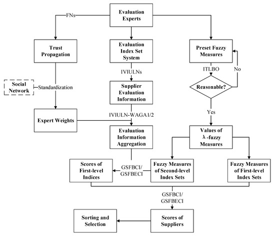
Figure 1.
Flowchart of the proposed model.
Step 1: Construction of the index system. Determine the index system based on existing research and experts’ discussion. Considering the lack of measurement of the -fuzzy measure, the index system includes two levels. There is a mutual relationship between first-level indices, and second-level indices under each first-level index should also have redundant interactions.
Step 2: Evaluation information acquisition. Based on the historical performance of suppliers, determine the objective values of all quantifiable indices for the suppliers. After that, score the performance of alternative suppliers under different indices. During the scoring process, experts are allowed to discuss, and their opinions can be modified on the spot. The scoring results of experts are recorded through IVIULNs, and each expert needs to evaluate the performance of suppliers in indices.
Step 3: Expert weights obtained by social network. FN is used to represent the trust relationship between experts. FN is a fuzzy number, which can be expressed as , where and represent the membership and non-membership of , respectively. In this process, it is necessary to first calculate the trust propagation relationship, and then then of each expert can be obtained through Equations (10)–(12). We can solve the weight of each expert through standardized transformation.
Step 4: Solutions of fuzzy measures for index sets. Based on the fuzzy measures given by experts for partial index sets, the NTLBO algorithm is used to solve them. It can be foreseen that if experts make incorrect evaluations during the process of preset fuzzy measures, the results will have significant errors. In this case, new fuzzy measures should be pre-assigned. When the error is controlled within a reasonable range, the fuzzy measures of all index sets can be obtained through Equation (6).
Step 5: Evaluation information aggregation. For the subjective evaluation information obtained in Step 2 and Step 3, use IVIULN-WAGA1 or IVIULN-WAGA2 to aggregate the evaluation information. Calculate the expected value using Equation (4). To eliminate the effect of dimensions and ensure all results are positive, the expected value is normalized using min-max scaling to a range of 0.5 to 1. Then, the expected value of all alternatives under the index can be calculated.
Step 6: Sorting and selection. This step is divided into two stages. First, it is necessary to examine the performance of the suppliers under each first-level index and then examine the overall performance of each supplier. Both stages can be obtained through Equations (21) and (22), where the value of the real value function is the expected value in step 5, and the fuzzy measures of index sets are obtained through step 4. According to the final scores of alternatives, select the best supplier.
Step 7: Discussion and sensitivity analysis. Discuss the results obtained from the model and analyze the sensitivity of the key parameters involved in the model.
5. Case Study
The proposed model will undergo empirical validation through a case study of a Chinese enterprise. Company A is an enterprise that provides digital services for government and enterprises. Its main business involves software service development, digital bidding and procurement, and the smart construction site. Currently, it has more than 20 regional branches. The regional branch located in Shanghai has recently taken over a project relating to a smart construction site. To achieve environmental protection goals, it needs to evaluate and select material suppliers. After preliminary screening, six alternative suppliers have been identified. There are a total of four experts participating in the evaluation, including the principal of the client, the manager of the project, the head of the project management department, and the liaison personnel of the PMO.
5.1. Weights of Experts
is a matrix composed of FNs representing direct trust propagation.
Except for the diagonal, if there is no FN at a corresponding position on the matrix, it indicates that there is no direct trust propagation between these two experts. For example, the principal of the client directly interacts with the project team members of Company A, so he has a direct trust propagation relationship with the manager of the project, while there is no trust propagation relationship with the head of the project management department and the liaison personnel of the PMO. To reveal the trust propagation relationship among all experts, experts with no direct trust propagation will form a trust propagation relationship through another expert. For example, to obtain a trust relationship from to , the propagation path is . The FN between and can be obtained from Equation (10).
Similarly, the complete trust propagation matrix can be obtained through calculation.
According to Equation (11), the trust score matrix is as follows:
Then, can be obtained:
So, the final weight of experts is , , , . In this case, is the most trusted and has the highest weight.
5.2. Fuzzy Measures of Index Sets
By consulting experts and discussing and referring to previous research [68,69,70,71,72,73,74,75], an evaluation index system was designed, as shown in Figure 2.
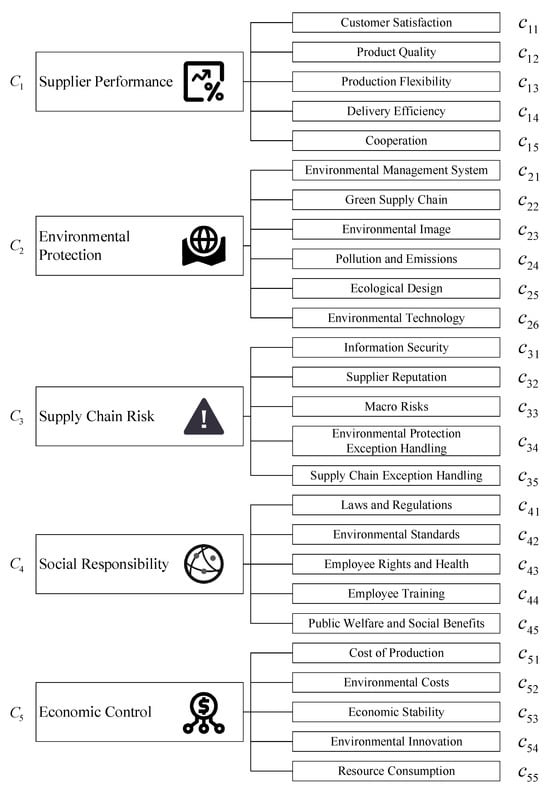
Figure 2.
Index system of green suppliers.
The index system includes a total of 5 first-level indices and 26 s-level indices. To ensure the objectivity of the case data, relevant indices were quantified based on the historical performance of the alternative suppliers. For data that cannot be quantified, such as customer satisfaction, experts will assign subjective scores based on their evaluation and discussions with the suppliers. The indices that require quantification and their descriptions are shown in Table 2. When calculating, it is necessary to handle them level by level. To save space, only the fuzzy measures of the second-level index sets under environmental protection are provided here to illustrate this process.
Table 2.
The quantitative indices, units, and descriptions.
The initial preset fuzzy measures for the index sets by experts are shown in Table 3.
Table 3.
Initial fuzzy measures of environmental protection.
Note that population size , the number of iterations , and the accuracy factors and are set to 500, 3000, 0.95, and 0.4, respectively. To compare the performance of the proposed algorithm, we compare relevant algorithms, mainly the TLBO algorithm, the ITLBO algorithm by Tian et al. [63], and the genetic algorithm. Each algorithm runs 20 times and records the results, as shown in the Table 4.
Table 4.
Comparison of different algorithms.
It can be observed that the proposed algorithm performs outstandingly and has significantly improved the performance of the existing TLBO. As one of the classic optimization algorithms, the genetic algorithm is much worse than NTLBO in terms of running time. The comparison results validate the effectiveness of the proposed algorithm.
Next, based on the fuzzy measures obtained from NTLBO operation , and , we can calculate the fuzzy measures of all index sets, as shown in Table 5.
Table 5.
Fuzzy measures of index set.
5.3. Sorting and Results
The initial evaluation data are , representing the evaluation made by the experts on all second-level indices under environmental protection. The specific evaluation information is shown as follows. Among them, is an objective figure derived from the supplier’s historical performance. In addition, the input from all experts are IVIULNs. This paper employs a 9-level scale method to assess each supplier based on the constructed index system, where the and represent the worst and best performance of the suppliers evaluated under this index, respectively. In the evaluation process, the degree of hesitation in the experts’ evaluation language will be represented by membership and non-membership, and the uncertainty can be represented by the width of the interval and numerical values.
Based on evaluation information and the weights of four experts, aggregate evaluation information by IVIULN-WAGA1 or IVIULN-WAGA2. Furthermore, through Equation (4), the expected values can be obtained. Subsequently, the expected value and the objective evaluation value of are normalized using min-max scaling, with their range controlled between 0.5 and 1 to prevent the situation where all results are 0 when sorting using GSFBECI. Thus, when the adjustment coefficient , IVIULN-WAGA1 is used for aggregation, and the normalized expected values of the six alternatives under six s-level environmental protection indices are as Table 6.
Table 6.
The normalized expected value after aggregation (IVIULN-WAGA1).
When using IVIULN-WAGA2, the result is shown in Table 7.
Table 7.
The normalized expected value after aggregation (IVIULN-WAGA2).
When , according to Equations (21) and (22), the GSFBCI and GSFBECI of all alternatives can be obtained, as shown in Table 8.
Table 8.
Suppliers’ scores in environmental protection.
The results show that after using different aggregation methods and different Choquet integrals, the ranking of all suppliers in terms of environmental protection is . This indicates that the aggregation method and sorting calculation proposed in this paper can achieve more stable results. Meanwhile, it is believed that Supplier has the most outstanding environmental performance, while Supplier has the worst performance in this area.
By using the above method to calculate the scores of other first-level indices, the performance of all alternatives under each first-level index can be obtained. To save space, the data displayed here are taken as an example of GSFBCI aggregated by IVIULN-WAGA1, as shown in Figure 3.
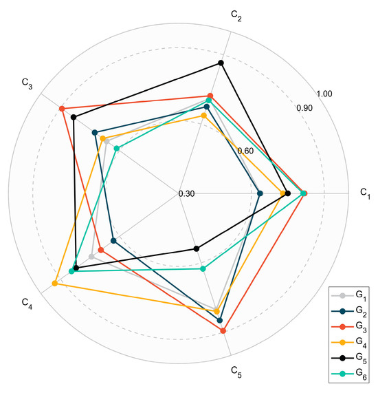
Figure 3.
Suppliers’ scores under first-level indices.
According to the radar chart, performs relatively evenly in all indices, while suppliers , , and have obvious strengths and weaknesses. In terms of economic control, receives significantly higher score, but performs poorly in other indices. performs well in all aspects, especially in the index of supply chain risk and economic control. Interestingly, the pentagon formed by completely covers .
Finally, using the obtained CI score as the expected value, GSFBCI and GSFBECI were recalculated. The results obtained using different aggregation methods and CI calculation methods are shown in Table 9.
Table 9.
Suppliers’ final scores.
5.4. Discussion
All results categorize the suppliers into two distinct categories, with suppliers , and scoring higher and suppliers , and scoring lower. It can be observed that the results of the second ranking using GSFBCI indicate , while GSFBECI concludes . This is because when calculating CI, it is necessary to arrange the indices in a certain order. By observing the radar chart, it is found that suppliers and each have their own strengths and weaknesses. However, when calculating GSFBECI, their strengths and weaknesses each correspond to specific exponents, and the calculation method of power increases the gap between the two. Similarly, it can be observed that under different aggregation operators, subtle differences in the ranking results also arise. Specifically, the score differences between suppliers and are smaller when using the IVIULN-WAGA2 aggregation compared to the IVIULN-WAGA1. As a result, when aggregating with IVIULN-WAGA2, the two rankings using GSFBCI conclude , while in all other cases, the results are . This may be due to the fact that when using IVIULN-WAGA2, if any expert evaluates the lower point of non-membership degree as 0, according to the aggregation equation, regardless of how other experts evaluate non-membership degree, the results will be 0. However, supplier has more experts who give the lower point of the non-membership degree as 0, so it will have higher expected values after aggregation. Regardless of the aggregation method and CI calculation method chosen, all results prove that Supplier is the optimal supplier in this case.
5.5. Sensitivity Analysis
To further analyze the impact of parameters on the sorting results, sensitivity analysis will be conducted on the key parameters in the model in this section to examine how they will affect the results.
Figure 4 shows the changes in the scores of each alternative as the parameters change when . The CI calculation method is GSFBCI through IVIULN-WAGA1 aggregation.
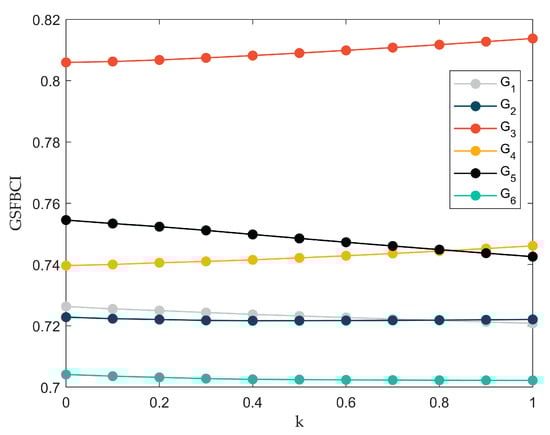
Figure 4.
Suppliers’ scores under different
(, IVIULN-WAGA1, GSFBCI, GSFBCI).
Observing Figure 4, it can be seen that with the variation of parameter , the scores of the alternative suppliers do not change significantly overall. When is around , the scores of supplier and and supplier and are very close, and their rankings will change. This figure indicates that the WAA aggregation operator tends to believe is preferred over and is superior to , whereas the WGA operator exhibits the opposite preference.
To examine the impact of parameter on the results and to analyze the score changes of suppliers and as discussed in Section 5.4, Figure 5 is plotted. It can be observed from Figure 5 that as the parameter changes, the suppliers’ overall scores remain relatively stable. Specifically, the scores of suppliers and are very close, and by comparing the specific score data, it is evident that near , the ranking of supplier and supplier has changed.
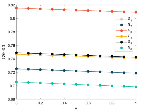
Figure 5.
Suppliers’ scores under different
(, IVIULN-WAGA2, GSFBCI, GSFBCI).
Next, the expert weights will be modified to , , , , to examine the robustness of the model under extreme conditions. The results can be seen in Table 10.
Table 10.
Suppliers’ final scores under extreme weight values.
Based on the results, it is not difficult to observe that under extreme expert weights, the model proposed in this paper should have strong robustness. Except for the discrepancies in the rankings of and due to different sorting methods, the ranking results of other suppliers are quite stable.
5.6. Suggestions for Countermeasures
The green supplier evaluation and selection model provides an important decision-making tool for enterprises in green supply chain management. This paper offers the following management insights and suggestions for managers:
- This research comprehensively evaluates the economic and environmental factors of green suppliers, enabling enterprises to balance cost-effectiveness while prioritizing suppliers’ performance in energy conservation and emission reduction.
- When evaluating and selecting green suppliers, enterprises should recognize potential synergistic effects or conflicting relationships among indices and fully account for interactions between evaluation indices.
- In interpreting expert evaluation language, inherent uncertainty must be identified while ensuring the stability of aggregation operators for evaluation language sets under extreme scenarios.
- The expert social network proposed in this study effectively quantifies trust relationships and mitigates individual experiential biases. The improved heuristic algorithm significantly enhances computational efficiency and can be applied to complex settings.
- The application of bi-directional Shapley–Choquet integrals quantifies interactions between indices, assisting enterprises in identifying suppliers that focus solely on single-aspect improvements.
In the current business environment, characterized by green transition and uncertainty, enterprises must establish scientific green supply chain management systems. By holistically considering economic and environmental factors, emphasizing interactions among indices, optimizing information aggregation operator, and employing quantitative calculations, this study offers insights and recommendations to help enterprises select and manage green suppliers while advancing sustainable development goals.
6. Conclusions, Limitations and Future Research
6.1. Conclusions
This study develops a multi-criteria decision-making model using IVIULN and bi-directional Shapley–Choquet integrals to evaluate and select green suppliers in uncertain environments. The proposed mathematical model can be employed in scenarios where expert information and evaluation criteria are unknown, while comprehensively considering the interactions among indices. The research demonstrates the following theoretical and practical contributions.
- This paper uses IVIULN to handle the uncertainty in the process of evaluation. An aggregation operator based on IVIULN is proposed, which compensates for the shortcomings of existing aggregation operators and improves the stability of evaluation results.
- This paper combines fuzzy measures with bi-directional Shapley–Choquet integrals, fully revealing the interrelationships between indices. At the same time, the establishment of a second level index system compensates for the shortcomings of the λ-fuzzy measure, which can only represent a set of fuzzy measures of indices.
- This paper improves the TLBO algorithm by introducing the idea of teaching students in accordance with their aptitude and incorporating a self-learning stage. This approach improves the algorithm’s global search capability. At the same time, the teaching stage is improved.
- A universal MCDM model is proposed, which helps decision makers achieve effective and reasonable evaluations. This model also hopes to better promote the development of green suppliers, thereby standardizing and supervising the construction of a good full process green supply chain.
At the same time, the paper also points out that when different aggregation operators or sorting methods are used for calculations, the results can be affected. This requires experts to pay attention to the lower bounds of membership/non-membership during the scoring process. Similarly, when calculating the GSFBECI, attention should also be paid to the selection of the real-valued functions. Sensitivity analysis shows that the adjustment coefficient and might have an impact on the results. In cases where the data are extremely close, the determination of the adjustment coefficient should be approached with caution.
6.2. Limitations
This paper has effectively improved the existing MCDM models. However, the model proposed in this study still has certain limitations. First, as mentioned earlier, the aggregation operators proposed in this study still have certain drawbacks. Specifically, when the lower limit of the membership/non-membership degree is 0, the evaluation results obtained by the aggregation operators IVIULN-WAGA1/IVIULN-WAGA2 will be underestimated/overestimated. When the overall conditions of two candidate alternatives are extremely close, this situation may lead to different results from the two aggregation operators. Second, the paper should explore further interaction and integration with other fields, such as the combination of game theory and MCDM models. Additionally, the paper focuses only on the upstream part of the supply chain. However, green supply chain management should be viewed as a holistic concept, and future research should take a comprehensive approach, considering the entire supply chain. Overall, the model proposed in this study has made an effective attempt at evaluating and selecting green suppliers. However, to further enhance the accuracy and practical significance of the model, the aforementioned drawbacks must be addressed.
6.3. Future Research
Green supply chain management has become an essential component of sustainable development phase for enterprises. Similarly, the process of green development does not merely encompass the raw material procurement stage. In the future, the proposed model could be extended to comprehensive evaluation and optimization of the entire green supply chain, thereby achieving further enhancement of the enterprise’s supply chain management and sustainability capabilities. Moreover, the integration of game theory and MCDM models can be considered to further advance research in the field of green supply chain management [76]. Additionally, in the process of supply chain management, the performance of suppliers is influenced by a variety of dynamic factors. Technologies such as machine learning could be integrated with the model. By learning from the historical performance of suppliers, these technologies can predict future trends and incorporate the prediction results into the supplier evaluation process. Green supply chain management involves the integration of multiple disciplines, such as economics and environmental science. By assessing the economic and environmental performance data of suppliers, the scientific validity and practical applicability of the model can be further enhanced.
Author Contributions
Conceptualization, W.Z. and Y.G.; methodology, Y.G.; software, Y.G.; validation, W.Z. and Y.G.; formal analysis, W.Z.; investigation, W.Z.; writing—original draft preparation, W.Z. and Y.G.; writing—review and editing, W.Z.; visualization, Y.G.; supervision, W.Z. All authors have read and agreed to the published version of the manuscript.
Funding
This research received no external funding.
Institutional Review Board Statement
Not applicable.
Informed Consent Statement
Not applicable.
Data Availability Statement
Data will be made available on request.
Conflicts of Interest
The authors declare no conflicts of interest.
Abbreviations
The following abbreviations are used in this manuscript:
| MCDM | Multi-criteria decision-making |
| IVIULN | Interval-valued intuitive uncertainty language number |
| NTLBO | Novel teaching-learning-based optimization |
| WA | Weighted average |
| WG | Weighted geometry |
References
- Zhang, L.; Liu, R.; Liu, H.; Shi, H. Green Supplier Evaluation and Selections: A State-of-the-Art Literature Review of Models, Methods, and Applications. Math. Probl. Eng. 2020, 2020, 1783421. [Google Scholar] [CrossRef]
- Maditati, D.R.; Munim, Z.H.; Schramm, H.-J.; Kummer, S. A Review of Green Supply Chain Management: From Bibliometric Analysis to a Conceptual Framework and Future Research Directions. Resour. Conserv. Recycl. 2018, 139, 150–162. [Google Scholar] [CrossRef]
- Fahimnia, B.; Sarkis, J.; Davarzani, H. Green Supply Chain Management: A Review and Bibliometric Analysis. Int. J. Prod. Econ. 2015, 162, 101–114. [Google Scholar] [CrossRef]
- Wen, D.; Sun, X.; Liu, Y. Bibliometric Analysis of Supplier Management: The Theme and Cluster Perspectives. Sustainability 2020, 12, 2572. [Google Scholar] [CrossRef]
- Abbasi, S.; Abbaspour, S.; Eskandari Nasab Siahkoohi, M.; Yousefi Sorkhi, M.; Ghasemi, P. Supply Chain Network Design Concerning Economy and Environmental Sustainability: Crisis Perspective. Results Eng. 2024, 22, 102291. [Google Scholar] [CrossRef]
- Khulud, K.; Masudin, I.; Zulfikarijah, F.; Restuputri, D.P.; Haris, A. Sustainable Supplier Selection through Multi-Criteria Decision Making (MCDM) Approach: A Bibliometric Analysis. Logist. Basel 2023, 7, 96. [Google Scholar] [CrossRef]
- Jeevan, J.; Salleh, N.H.M.; Kevin, N.H.A.C.K. An Environmental Management System in Seaports Evidence from Malaysia. Marit. Policy Manag. 2022, 50, 1118–1135. [Google Scholar] [CrossRef]
- Orji, I.J.; Kusi-Sarpong, S.; Huang, S.F.; Vazquez-Brust, D. Evaluating the Factors that Influence Blockchain Adoption in the Freight Logistics Industry. Transp. Res. Part E-Logist. Transp. Rev. 2020, 141, 26. [Google Scholar] [CrossRef]
- Oubahman, L.; Duleba, S. Review of Promethee Method in Transportation. Prod. Eng. Arch. 2021, 27, 69–74. [Google Scholar] [CrossRef]
- Çelikbilek, Y.; Tüysüz, F. An in-Depth Review of Theory of the TOPSIS Method: An Experimental Analysis. J. Manag. Anal. 2020, 7, 281–300. [Google Scholar] [CrossRef]
- Hsu, C.-W.; Kuo, T.-C.; Chen, S.-H.; Hu, A.H. Using Dematel to Develop a Carbon Management Model of Supplier Selection in Green Supply Chain Management. J. Clean. Prod. 2013, 56, 164–172. [Google Scholar] [CrossRef]
- Büyüközkan, G.; Güleryüz, S. An Integrated Dematel-Anp Approach for Renewable Energy Resources Selection in Turkey. Int. J. Prod. Econ. 2016, 182, 435–448. [Google Scholar] [CrossRef]
- Basheleishvili, I. Developing the Expert Decision-Making Algorithm Using the Methods of Multi-Criteria Analysis. Cybern. Inf. Technol. 2020, 20, 22–29. [Google Scholar] [CrossRef]
- Chen, N.; Cai, J.; Ma, Y.; Han, W. Green Supply Chain Management under Uncertainty: A Review and Content Analysis. Int. J. Sustain. Dev. World Ecol. 2021, 29, 349–365. [Google Scholar] [CrossRef]
- Islam, M.S.; Tseng, M.-L.; Karia, N.; Lee, C.-H. Assessing Green Supply Chain Practices in Bangladesh Using Fuzzy Importance and Performance Approach. Resour. Conserv. Recycl. 2018, 131, 134–145. [Google Scholar] [CrossRef]
- Peng, J.J.; Chen, X.G.; Wang, X.K.; Wang, J.Q.; Long, Q.Q.; Yin, L.J. Picture Fuzzy Decision-Making Theories and Methodologies: A Systematic Review. Int. J. Syst. Sci. 2023, 54, 2663–2675. [Google Scholar] [CrossRef]
- Wu, J.; Chiclana, F.; Fujita, H.; Herrera-Viedma, E. A Visual Interaction Consensus Model for Social Network Group Decision Making with Trust Propagation. Knowl. Based Syst. 2017, 122, 39–50. [Google Scholar] [CrossRef]
- Singh, M.; Pant, M. A Review of Selected Weighing Methods in MCDM with a Case Study. Int. J. Syst. Assur. Eng. Manag. 2020, 12, 126–144. [Google Scholar] [CrossRef]
- Zhang, L.; Xu, Y.; Yeh, C.-H.; Liu, Y.; Zhou, D. City Sustainability Evaluation Using Multi-Criteria Decision Making with Objective Weights of Interdependent Criteria. J. Clean. Prod. 2016, 131, 491–499. [Google Scholar] [CrossRef]
- Sałabun, W.; Wątróbski, J.; Shekhovtsov, A. Are Mcda Methods Benchmarkable? A Comparative Study of TOPSIS, Vikor, Copras, and Promethee II Methods. Symmetry 2020, 12, 1549. [Google Scholar] [CrossRef]
- Wang, J.-J.; Jing, Y.-Y.; Zhang, C.-F.; Shi, G.-H.; Zhang, X.-T. A Fuzzy Multi-Criteria Decision-Making Model for Trigeneration System. Energy Policy 2008, 36, 3823–3832. [Google Scholar] [CrossRef]
- Basílio, M.P.; Pereira, V.; Costa, H.G.; Santos, M.; Ghosh, A. A Systematic Review of the Applications of Multi-Criteria Decision Aid Methods (1977–2022). Electronics 2022, 11, 1720. [Google Scholar] [CrossRef]
- Tian, G.; Lu, W.; Zhang, X.; Zhan, M.; Dulebenets, M.A.; Aleksandrov, A.; Fathollahi-Fard, A.M.; Ivanov, M. A Survey of Multi-criteria Decision-Making Techniques for Green Logistics and Low-Carbon Transportation Systems. Environ. Sci. Pollut. Res. 2023, 30, 57279–57301. [Google Scholar] [CrossRef]
- Jorm, A.F. Using the Delphi Expert Consensus Method in Mental Health Research. Aust. N. Z. J. Psychiatry 2015, 49, 887–897. [Google Scholar] [CrossRef]
- Chatterjee, K.; Pamucar, D.; Zavadskas, E.K. Evaluating the Performance of Suppliers Based on Using the R’amatel-Mairca Method for Green Supply Chain Implementation in Electronics Industry. J. Clean. Prod. 2018, 184, 101–129. [Google Scholar] [CrossRef]
- Liou, J.J.H.; Chuang, Y.-C.; Zavadskas, E.K.; Tzeng, G.-H. Data-Driven Hybrid Multiple Attribute Decision-Making Model for Green Supplier Evaluation and Performance Improvement. J. Clean. Prod. 2019, 241, 118321. [Google Scholar] [CrossRef]
- Qu, G.; Zhang, Z.; Qu, W.; Xu, Z. Green Supplier Selection Based on Green Practices Evaluated Using Fuzzy Approaches of TOPSIS and Electre with a Case Study in a Chinese Internet Company. Int. J. Environ. Res. Public Health 2020, 17, 3268. [Google Scholar] [CrossRef]
- Qin, Y.; Xu, Z.S.; Wang, X.X.; Skare, M. Fuzzy Decision-Making in Tourism and Hospitality: A Bibliometric Review. J. Intell. Fuzzy Syst. 2024, 46, 4955–4980. [Google Scholar] [CrossRef]
- Fan, X.F.; Li, T. Fuzzy Switching Sliding Mode Control of T-S Fuzzy Systems Via an Event-Triggered Strategy. IEEE Trans. Fuzzy Syst. 2024, 32, 6172–6184. [Google Scholar] [CrossRef]
- Zadeh, L.A. Fuzzy sets. Inf. Comput. 1965, 8, 338–353. [Google Scholar]
- Kalmanson, D.; Stegall, H.F. Cardiovascular Investigations and Fuzzy Sets Theory. Am. J. Cardiol. 1975, 35, 80–84. [Google Scholar] [CrossRef]
- Bustince, H.; Barrenechea, E.; Pagola, M.; Fernandez, J.; Xu, Z.S.; Bedregal, B.; Montero, J.; Hagras, H.; Herrera, F.; De Baets, B. A Historical Account of Types of Fuzzy Sets and Their Relationships. IEEE Trans. Fuzzy Syst. 2016, 24, 179–194. [Google Scholar] [CrossRef]
- Babakordi, F. Arithmetic Operations on Generalized Trapezoidal Hesitant Fuzzy Numbers and Their Application to Solving Generalized Trapezoidal Hesitant Fully Fuzzy Equation. Int. J. Uncertain. Fuzziness Knowl. Based Syst. 2024, 32, 85–108. [Google Scholar] [CrossRef]
- Pakdel, M.; Razzaghnia, T.; Fathi, K.; Mostafaee, A. Estimation of Fuzzy Regression Parameters with Anfis and Bayesian Methods. Eng. Rep. 2025, 7, e13086. [Google Scholar] [CrossRef]
- Chen, L. Interval-Valued T-Spherical Fuzzy Extended Power Aggregation Operators and Their Application in Multi-Criteria Decision-Making. J. Intell. Syst. 2024, 33, 20240039. [Google Scholar] [CrossRef]
- Xu, C.L.; Lan, Y.S. An Improved Intuitionistic Fuzzy Entropy and Its Analysis. J. Nonlinear Convex Anal. 2024, 25, 1225–1236. [Google Scholar]
- Atanassov, K.; Gargov, G. Interval Valued Intutionistic Fuzzy Sets. Fuzzy Sets Syst. 1989, 31, 343–349. [Google Scholar]
- Bihari, R.; Jeevaraj, S.; Kumar, A. A New Simplex Algorithm for Interval-Valued Fermatean Fuzzy Linear Programming Problems. Comput. Appl. Math. 2024, 44, 44. [Google Scholar] [CrossRef]
- Li, L.; Hao, M. Interval-Valued Pythagorean Fuzzy Entropy and Its Application to Multi-Criterion Group Decision-Making. AIMS Math. 2024, 9, 12511–12528. [Google Scholar] [CrossRef]
- Liu, P.D. Some Geometric Aggregation Operators Based on Interval Intuitionistic Uncertain Linguistic Variables and Their Application to Group Decision Making. Appl. Math. Model. 2013, 37, 2430–2444. [Google Scholar] [CrossRef]
- Zhang, H.; Zhao, S.; Kou, G.; Li, C.-C.; Dong, Y.; Herrera, F. An Overview on Feedback Mechanisms with Minimum Adjustment or Cost in Consensus Reaching in Group Decision Making: Research Paradigms and Challenges. Inf. Fusion 2020, 60, 65–79. [Google Scholar] [CrossRef]
- Guo, J.; Liang, X.; Wang, L. Online Reviews-Oriented Hotel Selection: A Large-Scale Group Decision-Making Method Based on the Expectations of Decision Makers. Appl. Intell. 2022, 53, 16347–16366. [Google Scholar] [CrossRef]
- Herrera-Viedma, E.; Palomares, I.; Li, C.-C.; Cabrerizo, F.J.; Dong, Y.; Chiclana, F.; Herrera, F. Revisiting Fuzzy and Linguistic Decision Making: Scenarios and Challenges for Making Wiser Decisions in a Better Way. IEEE Trans. Syst. Man Cybern. Syst. 2021, 51, 191–208. [Google Scholar] [CrossRef]
- Dong, Y.; Zhao, S.; Zhang, H.; Chiclana, F.; Herrera-Viedma, E. A Self-Management Mechanism for Noncooperative Behaviors in Large-Scale Group Consensus Reaching Processes. IEEE Trans. Fuzzy Syst. 2018, 26, 3276–3288. [Google Scholar] [CrossRef]
- Zhang, H.; Palomares, I.; Dong, Y.; Wang, W. Managing Non-Cooperative Behaviors in Consensus-Based Multiple Attribute Group Decision Making: An Approach Based on Social Network Analysis. Knowl. Based Syst. 2018, 162, 29–45. [Google Scholar] [CrossRef]
- Zhang, Z.; Gao, Y.; Li, Z. Consensus Reaching for Social Network Group Decision Making by Considering Leadership and Bounded Confidence. Knowl. Based Syst. 2020, 204, 106240. [Google Scholar] [CrossRef]
- Zahedi Khameneh, A.; Kilicman, A. Some Construction Methods of Aggregation Operators in Decision-Making Problems: An Overview. Symmetry 2020, 12, 694. [Google Scholar] [CrossRef]
- Akram, M.; Dudek, W.A.; Ilyas, F. Group Decision-Making Based on Pythagorean Fuzzy TOPSIS Method. Int. J. Intell. Syst. 2019, 34, 1455–1475. [Google Scholar] [CrossRef]
- Dawlet, O.; Bao, Y.-L. Normalized Hesitant Fuzzy Aggregation Operators for Multiple Attribute Decision-Making. Int. J. Fuzzy Syst. 2024, 26, 1982–1997. [Google Scholar] [CrossRef]
- Zeng, S.; Zhang, N.; Zhang, C.; Su, W.; Carlos, L.-A. Social Network Multiple-Criteria Decision-Making Approach for Evaluating Unmanned Ground Delivery Vehicles under the Pythagorean Fuzzy Environment. Technol. Forecast. Soc. Chang. 2022, 175, 121414. [Google Scholar] [CrossRef]
- Chen, T.; Wang, J. Identification of λ-Fuzzy Measures Using Sampling Design and Genetic Algorithms. Fuzzy Sets Syst. 2001, 123, 321–341. [Google Scholar] [CrossRef]
- Grubb, D.; Laberge, T. Additivity of Quasi-Measures. Proc. Amer. Math. Soc. 1998, 126, 3007–3012. [Google Scholar] [CrossRef]
- Degan, Z.; Hongtao, P.; Guocheng, Y.I.N.; Guangping, Z.; Yixin, Y.I.N. Approach of Belief Measure Based on Fuzzy-Neural Network for Proactive service. Control Decis. 2006, 21, 258–262. [Google Scholar]
- Ma, S.; Li, S. Complex Fuzzy Set-Valued Complex Fuzzy Measures and Their Properties. Sci. World J. 2014, 2014, 493703. [Google Scholar] [CrossRef]
- Beliakov, G.; Baz, J.; Wu, J.-Z. Efficient random Walks for Generating Random Fuzzy Measures in Möbius Representation in Large Universe. Comput. Appl. Math. 2024, 43, 430. [Google Scholar] [CrossRef]
- Wu, X.; Feng, Y.; Lou, S.; Li, Z.; Hu, B.; Hong, Z.; Si, H.; Tan, J. A Multi-Criteria Decision-Making Approach for Pressurized Water Reactor Based on Hesitant Fuzzy-Improved Cumulative Prospect Theory and 2-Additive Fuzzy Measure. J. Ind. Inf. Integr. 2024, 40, 100631. [Google Scholar] [CrossRef]
- Mane, A.; Dongale, T.; Bapat, M. Application of Fuzzy Measure and Fuzzy Integral in Students Failure Decision Making. IOSR J. Math. 2014, 10, 47–53. [Google Scholar]
- Wan, S.-P.; Yan, J.; Zou, W.-C.; Dong, J.-Y. Generalized Shapley Choquet Integral Operator Based Method for Interactive Interval-Valued Hesitant Fuzzy Uncertain Linguistic Multi-Criteria Group Decision Making. IEEE Access 2020, 8, 202194–202215. [Google Scholar] [CrossRef]
- Meng, F.; Chen, S.-M.; Tang, J. Multicriteria Decision Making Based on Bi-Direction Choquet Integrals. Inf. Sci. 2021, 555, 339–356. [Google Scholar] [CrossRef]
- Wang, H.; Liu, Y.; Zhao, C. Q-Rung Orthopair Fuzzy Bi-Direction Choquet Integral Based on TOPSIS Method for Multiple Attribute Group Decision Making. Comput. Appl. Math. 2023, 42, 105. [Google Scholar] [CrossRef]
- Weng, L.; Lin, J.; Lv, S.J.; Huang, Y. A Bi-Direction Performance Evaluation Model for Water Pollution Treatment Engineering under the Intuitionistic Multiplicative Linguistic Environment. J. Intell. Fuzzy Syst. 2023, 44, 4149–4173. [Google Scholar] [CrossRef]
- Shi, H.; Quan, M.-Y.; Liu, H.-C.; Duan, C.-Y. A Novel Integrated Approach for Green Supplier Selection with Interval-Valued Intuitionistic Uncertain Linguistic Information: A Case Study in the Agri-Food Industry. Sustainability 2018, 10, 733. [Google Scholar] [CrossRef]
- Tian, G.; Hao, N.; Zhou, M.; Pedrycz, W.; Zhang, C.; Ma, F.; Li, Z. Fuzzy Grey Choquet Integral for Evaluation of Multicriteria Decision Making Problems with Interactive and Qualitative Indices. IEEE Trans. Syst. Man Cybern.-Syst. 2020, 51, 1855–1868. [Google Scholar] [CrossRef]
- Meng, F.; Chen, X.; Zhang, Q. Some Interval-Valued Intuitionistic Uncertain Linguistic Choquet Operators and Their Application to Multi-Attribute Group Decision Making. Appl. Math. Model. 2014, 38, 2543–2557. [Google Scholar] [CrossRef]
- Ye, J. Intuitionistic Fuzzy Hybrid Arithmetic and Geometric Aggregation Operators for the Decision-Making of Mechanical Design Schemes. Appl. Intell. 2017, 47, 743–751. [Google Scholar] [CrossRef]
- Onisawa, T.; Sugeno, M.; Nishiwaki, Y.; Kawai, H.; Harima, Y. Fuzzy Measure Analysis of Public Attitude Towards the Use of Nuclear energy. Fuzzy Sets Syst. 1986, 20, 259–289. [Google Scholar]
- Marichal, J.-L. The Influence of Variables on Pseudo-Boolean Functions with Applications to Game Theory and Multicriteria Decision Making. Discret Appl. Math. 2000, 107, 139–164. [Google Scholar] [CrossRef]
- Lo, H.-W.; Liou, J.J.H.; Wang, H.-S.; Tsai, Y.-S. An Integrated Model for Solving Problems in Green Supplier Selection and Order Allocation. J. Clean. Prod. 2018, 190, 339–352. [Google Scholar] [CrossRef]
- Shang, Z.; Yang, X.; Barnes, D.; Wu, C. Supplier Selection in Sustainable Supply Chains: Using the Integrated BWM, Fuzzy Shannon Entropy, and Fuzzy Multimoora Methods. Expert Syst. Appl. 2022, 195, 116567. [Google Scholar] [CrossRef]
- Dos Santos, B.M.; Godoy, L.P.; Campos, L.M.S. Performance Evaluation of Green Suppliers Using Entropy-TOPSIS-F. J. Clean. Prod. 2019, 207, 498–509. [Google Scholar] [CrossRef]
- Liou, J.J.H.; Chang, M.-H.; Lo, H.-W.; Hsu, M.-H. Application of an MCDM Model with Data Mining Techniques for Green Supplier Evaluation and Selection. Appl. Soft. Comput. 2021, 109, 107534. [Google Scholar] [CrossRef]
- Masoomi, B.; Sahebi, I.G.; Fathi, M.; Yıldırım, F.; Ghorbani, S. Strategic Supplier Selection for Renewable Energy Supply Chain under Green Capabilities (Fuzzy Bwm-Waspas-Copras Approach). Energy Strateg. Rev. 2022, 40, 100815. [Google Scholar] [CrossRef]
- Keshavarz-Ghorabaee, M.; Amiri, M.; Hashemi-Tabatabaei, M.; Zavadskas, E.K.; Kaklauskas, A. A New Decision-Making Approach Based on Fermatean Fuzzy Sets and Waspas for Green Construction Supplier Evaluation. Mathematics 2020, 8, 2202. [Google Scholar] [CrossRef]
- Verma, M.; Prem, P.R.; Ren, P.; Liao, H.; Xu, Z. Green Supplier Selection with a Multiple Criteria Decision-Making Method Based on Thermodynamic Features. Environ. Dev. Sustain. 2022. [Google Scholar] [CrossRef]
- Kara, K.; Acar, A.Z.; Polat, M.; Önden, İ.; Cihan Yalçın, G. Developing a Hybrid Methodology for Green-Based Supplier Selection: Application in the Automotive Industry. Expert Syst. Appl. 2024, 249, 123668. [Google Scholar] [CrossRef]
- Su, C.; Deng, J.; Li, X.; Huang, W.; Ma, j.; Wang, C.; Wang, X. Investment in Enhancing Resilience Safety of Chemical Parks under Blockchain Technology: From the Perspective of Dynamic Reward and Punishment Mechanisms. J. Loss Prev. Process Ind. 2025, 94, 105523. [Google Scholar] [CrossRef]
Disclaimer/Publisher’s Note: The statements, opinions and data contained in all publications are solely those of the individual author(s) and contributor(s) and not of MDPI and/or the editor(s). MDPI and/or the editor(s) disclaim responsibility for any injury to people or property resulting from any ideas, methods, instructions or products referred to in the content. |
© 2025 by the authors. Licensee MDPI, Basel, Switzerland. This article is an open access article distributed under the terms and conditions of the Creative Commons Attribution (CC BY) license (https://creativecommons.org/licenses/by/4.0/).