Article

Untangling Carbon–Clean Energy Dynamics: A Quantile Granger-Causality Perspective

School of Economics, Qingdao University, Qingdao 266071, China
*
Author to whom correspondence should be addressed.
Sustainability 2025, 17(7), 3118; https://doi.org/10.3390/su17073118
Submission received: 4 February 2025 / Revised: 9 March 2025 / Accepted: 12 March 2025 / Published: 1 April 2025

Abstract

:
This study examines the dynamic relationship between carbon markets and clean energy stocks using a quantile Granger-causality framework, capturing nonlinear dependencies across different market conditions. Unlike conventional mean-based approaches, this method identifies asymmetric causal linkages, particularly during periods of extreme market movements. Empirical results reveal a bidirectional Granger-causal relationship between carbon price returns and clean energy stock returns, predominantly at the lower quantile τ = 0.25 and upper quantile τ = 0.75 of the conditional distribution. This indicates that carbon price fluctuations significantly impact clean energy investments during bullish (>0.50 quantiles) and bearish (<0.50 quantiles) trends, while the effect is weaker during stable periods (0.50 quantile). Additionally, findings suggest that the impact of carbon pricing varies across regions. While the signs of the Granger-causality running from carbon markets to clean energy stocks are less than 0 in global, European, and U.S. markets, China’s policy-driven sustainability initiatives mitigate these risks, enhancing investment stability. These findings underscore the importance of region-specific carbon policies in supporting clean energy growth. Policymakers should consider stabilization mechanisms in volatile markets and strategic carbon pricing to optimize investment incentives. Future research should explore the role of green financial innovations in enhancing carbon market efficiency and reducing investment uncertainty in clean energy transitions.

1. Introduction

The reduction of carbon emissions is a critical concern for supply chains and public policy due to the significant increase in greenhouse gas emissions, particularly CO2, which has intensified global warming [1,2,3]. To address climate change, some countries have established carbon dioxide emission restrictions, including carbon allowance programs [4,5,6]. To attain low-carbon development, governments are concurrently promoting the generation and utilization of clean or low-carbon energy as substitutes for fossil fuels. The effectiveness of these carbon reduction initiatives may be undermined by the interaction between the carbon and renewable energy markets. Achieving low-carbon objectives becomes challenging if the reduction of carbon allowances adversely affects the clean energy sector. Consequently, for policymakers focused on low-carbon development, it is crucial to understand the interaction between the carbon and renewable energy markets.
Although several research have investigated the correlation between carbon markets and energy markets [7,8,9,10,11,12,13,14,15,16,17] or the association between EUAs and stock markets [18,19,20,21,22,23,24,25,26], there is a scarcity of analyses concerning clean energy stock prices. This study employs a Granger-causality framework in quantiles to investigate the dynamic link between carbon pricing and clean energy indices throughout the distribution. We choose EUA futures and four clean energy indices in different countries or dimensions—global, European, US, and Chinese—during the timeframe from January, 2012, to May, 2023. This period encompasses the final year of Phase II, the complete duration of Phase III, and the initial two and a half years of Phase IV of the EU ETS.
This paper aims to close the research gap by examining the Granger-causality in quantiles between EUAs and four clean energy stock indices. An extensive amount of research has been conducted to investigate the connection between carbon and traditional energy markets. The majority of these studies have concentrated on the prices of EUA and traditional energy [7,8,9,10,11,12,13,14,15,27,28], and they have consistently discovered a substantial association between the two. Another line of inquiry studies the relationship between energy prices and the stock prices of clean energy companies [29,30,31,32,33]. This line of inquiry focusses specifically on the substitution effect that exists between oil prices and clean energy indices [34,35,36,37,38,39,40,41,42].
There are still very few research that explicitly relate carbon markets with clean energy equities, and the conclusions of these studies are inconsistent. The findings of Kumar et al. [43] and Dutta [44] indicate that there is no statistical evidence of Granger-causation between EUA prices and U.S. clean energy indices. On the other hand, Dutta et al. [45] discovered a volatility nexus with European clean energy stocks. In contrast, Hanif et al. [46] and Tiwari et al. [47] revealed that EUAs are spillover receivers from clean energy stocks. Wang et al. [48] observed a positive association between EUA prices and clean energy indices. Both of these studies were conducted in the United States. These findings were further demonstrated by Mo et al. [49], who established that EUA prices have dynamic effects on the returns of green energy stock.
Nevertheless, current studies investigating the relationship between carbon prices and clean energy indices predominantly emphasize average effects, neglecting fluctuations across diverse market situations. Unlike conventional mean regression models that evaluate causality at the mean of the distribution, our approach searches causal links all around the entire conditional distribution including its tails. This difference is crucial since causal effects might only show up in very rare market environments. A parametric test which is put forward by Troster [50] is applied in our analysis to evaluate the causality between carbon market and clean energy stocks in all quantiles of the distribution, as opposed to focusing on an essential condition for Granger-causality—causality in mean. Compared to Chuang et al. [51] who test the quantile causal relations based on the specific specification of the quantile regression model by using the sup–Wald test proposed by Koenker and Machado [52], the test of Troster [50] needs only a marginal quantile regression model under the null hypothesis of noncausality. Moreover, compared with the nonparametric tests of Hong et al. [53] and Balcilar et al. [54], the parametric test of Troster [50] requires no mixing assumptions, and needs only less restrictive α-mixing assumptions for the validity of the subsampling. Therefore, this parametric test method is conducive to explore the causal effects on each quantile of the distribution and distinguish between causal relations in the distribution’s median and tails.
China has become the foremost clean energy market worldwide, investing USD 380 billion in 2021, succeeded by the European Union with USD 260 billion and the United States with USD 215 billion [55]. Since 2015, industrialized economies and China have propelled global renewable energy investments, whereas emerging and developing economies have experienced stagnation [56]. Although China excels in clean energy infrastructure, prior research predominantly emphasizes global, European, or U.S. indices, neglecting the interrelations between the EU ETS and China’s clean energy sector. It is noteworthy that only a small number of studies have investigated China’s clean energy business, despite the fact that China is the largest clean energy market in the world. This study fills this vacuum by adopting a quantile Granger-causality framework to investigate the asymmetric and region-specific relationship between carbon prices and clean energy stock returns. Specifically, the study focusses on clean energy stock returns. Through the identification of causal changes across a variety of market situations, our findings provide policymakers with significant insights that can be utilized in the formulation of carbon pricing and clean energy policies that are relevant to certain regions.
This study examines the research question: “How do fluctuations in carbon prices affect clean energy stock returns under varying market conditions, and do these effects differ by region?” Theoretically, there is a bidirectional relationship between carbon markets and clean energy stocks. Rising carbon prices increase compliance costs for high-emission industries. This incentivizes firms to adopt clean energy to reduce emissions, driving the performance of clean energy firms upward. In contrast, rapid scaling of renewables reduces fossil energy dependency, which weakens the demand for carbon allowances, potentially suppressing carbon prices if policy caps of emissions remain static. Additionally, surges in clean energy stock performance signal investor confidence in the energy transition. Investors may short carbon assets and increase the investment of clean energy assets, thereby influencing carbon price volatility. Furthermore, the policy environments may vary with different regions or countries (manifested as differentiated carbon trading mechanism, financial incentive, regulatory policy and so on), which results in the changes in the relations between the carbon market and clean energy stocks.
We utilize a quantile Granger-causality method to empirically analyze the evolution of the causal relationship between carbon pricing and clean energy stocks over the return distribution, especially in bullish and bearish market scenarios. We additionally evaluate if these consequences vary among global, European, U.S., and Chinese markets.
This study makes three key contributions:
  • Quantile-based insights—we examine the causal relationship between carbon markets and clean energy stocks across different quantiles, enabling policymakers to tailor strategies based on varying market conditions.
  • Regional specificity—by analyzing global, European, U.S., and Chinese clean energy indices, we identify region-specific causal effects. Notably, we explore the underexamined nexus between the EU ETS and China’s clean energy market.
  • Advanced methodology—using Troster’s quantile causality test, we investigate median and tail causality, offering a nuanced understanding of the carbon–clean energy relationship during Phases III and IV of the EU ETS.
Findings reveal a bidirectional Granger-causality between carbon prices and clean energy stocks in the conditional tails but not at the median. Additionally, the causal effects vary by region: while carbon markets negatively impact global, European, and U.S. clean energy stocks during bullish and bearish trends, they positively influence China’s clean energy stocks under similar conditions. These results offer essential direction for policymakers in formulating region-specific carbon and renewable energy strategies to facilitate low-carbon growth.
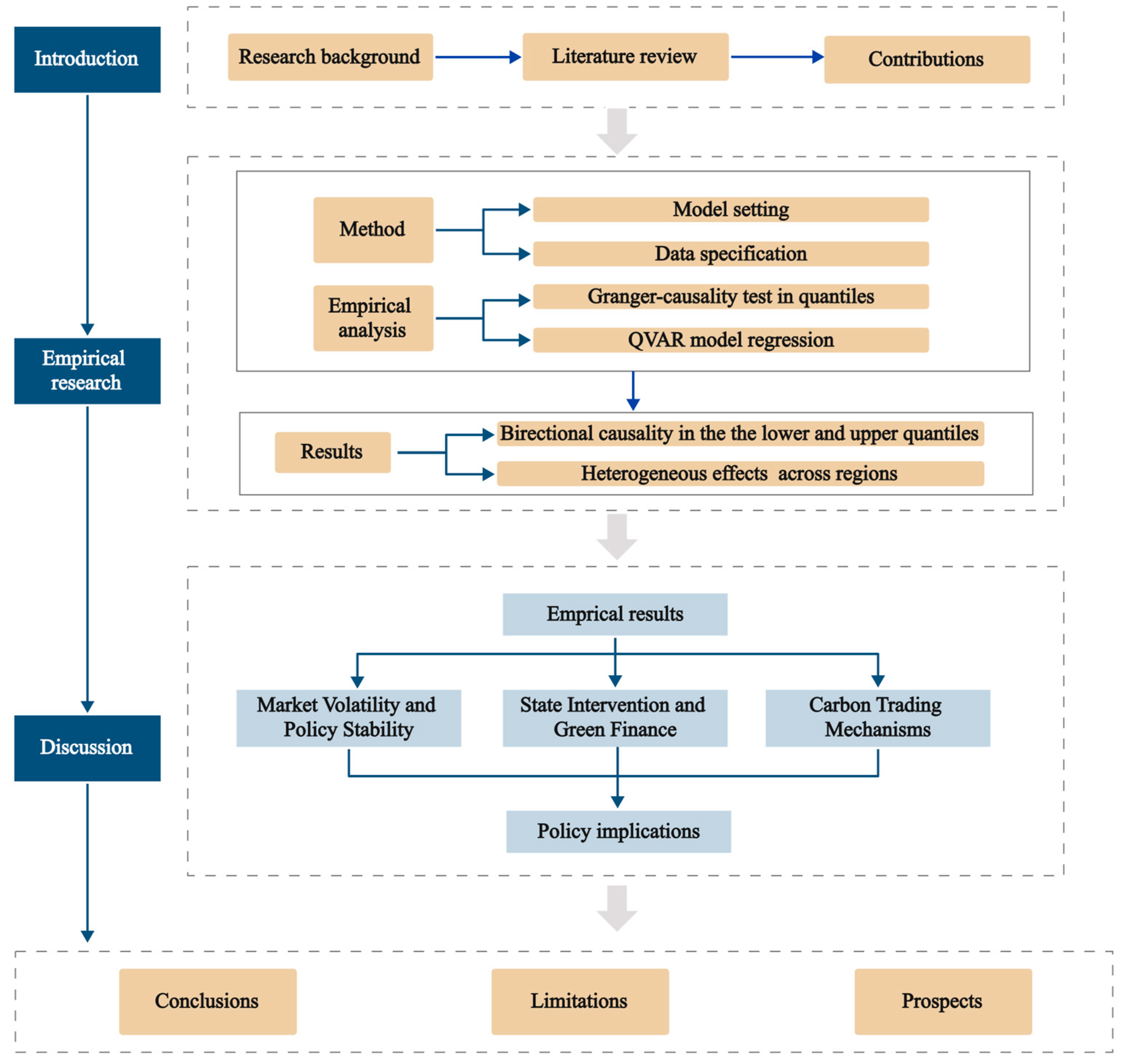
The subsequent sections of this work are structured as follows: Section 2 delineates the methodology and data, Section 3 gives the empirical analysis, Section 4 discusses the finishes with policy implications, and Section 5 concludes. Figure 1 depicts the research framework of this study.

2. Method

2.1. Quantile Granger Causality Testing

We consider an explanatory vector I t ( I t Y , I t Z ) R d , d = s + q , where I t Y : = ( Y t 1 , , Y t s ) R s , I t Z : = ( Z t 1 , , Z t q ) R q , and follow Chuang et al. [51] in defining that a random variable Z t is not Granger-caused by Y t at the conditional τ -quantile of Y t if:
H 0 QC Z Y : Q τ Y , Z Y t I t Y , I t Z = Q τ Y Y t I t Y ,   a . s .   for   all   τ T ,
where Q t Y , Z ( Y t | I t Y , I t Z ) denotes the τ -quantile of Y t , and T is a compact information set such that T [ 0 , 1 ] .

2.1.1. Null Hypothesis of Non-Granger-Causality

Following Troster [50], we redefine the null hypothesis as the following:
H 0 Z Y : E 1 Y t m I t Y , θ 0 τ I t Y , I t Z = τ ,   a . s .   for   all   τ T ,
where 1 [ a b ] is an indicator function, and the parametric quantile model m ( I t Y , θ 0 ( τ ) ) belongs to a group of functions M = { m ( I t Y , θ 0 ( τ ) ) | θ 0 ( ) : τ θ 0 ( τ ) Θ p .

2.1.2. Moment Condition Representation

According to Troster [50], the null hypothesis (2) can be equivalently expressed using the unconditional moment condition:
E 1 Y t m I t Y , θ 0 τ 0 τ exp i ω I t = 0 ,   for   all   τ T ,
where exp ( i ω I t ) : = exp [ i ( ω 1 ( Y t 1 , Z t 1 ) + + ω r ( Y t r , Z t r ) ) ] is a weight function, for all ω r with r d , and i = 1 is the imaginary root. Based on the sample analogue of E { [ 1 ( Y t m ( I t Y , θ 0 ( τ ) ) 0 ) τ ] exp ( i ω I t ) } , we define the residual process v T ( ω , τ ) , such that ω d and τ T as in the following:
v T ω , τ : = 1 T t = 1 T 1 Y t m I t Y , θ T τ 0 τ exp i ω I t ,
where θ T is a T -consistent estimator of θ 0 ( τ ) for all τ T .

2.1.3. Test Statistic Definition

The test statistic is formulated as the following:
S T : = T W v T ω , τ 2 d F ω ω d F τ τ ,
where F ω ( ) represents the conditional distribution function, and ω d follows a standard normal distribution. The test statistic estimation is as follows:
S T = 1 T n j = 1 n ψ × j W ψ × j ,
where W is a transformation matrix derived from residuals. A high S T value leads to rejecting the null hypothesis (2). Critical values are computed using the subsampling approach by Troster [50], with the subsample size b = [ k T 2 / 5 ] where k is a constant.

2.1.4. Parametric Quantile Autoregression (QVAR) Model

Following Troster et al. [57], we implement three parametric QAR models for testing Equation (6) under the null hypothesis Equation (2):
QAR 1 : m 1 I t Y , θ τ = μ 1 τ + μ 2 τ Y t 1 + σ t Φ u 1 τ , QAR 2 : m 2 I t Y , θ τ = μ 1 τ + μ 2 τ Y t 1 + μ 3 τ Y t 2 + σ t Φ u 1 τ , QAR 3 : m 3 I t Y , θ τ = μ 1 τ + μ 2 τ Y t 1 + μ 3 τ Y t 2 + μ 4 τ Y t 3 + σ t Φ u 1 τ ,
where the parameters θ ( τ ) = ( μ 1 ( τ ) , μ 2 ( τ ) , μ 3 ( τ ) , μ 4 ( τ ) , σ t ) are estimated via maximum likelihood. To examine the causal effects between the carbon and clean energy markets, we incorporate the lagged variables of the other time series into Equation (7) and estimate β ( τ ) across quantiles.
For simplicity, consistent with Troster et al. [57], we focus on results from the QAR (3) model:
Q τ Y Y t I t Y , I t Z = μ 1 τ + μ 2 τ Y t 1 + μ 3 τ Y t 2 + μ 4 τ Y t 3 + β τ Z t 1 + σ t Φ u 1 τ .

2.2. Data

We examine weekly data on carbon prices and four clean energy indices from 1 January 2012, to 7 May 2023, totaling 593 observations. The EUA futures price series (CP) from the Intercontinental Exchange (ICE) denotes carbon pricing, utilizing settlement prices from continuous contracts for the spot month. The clean energy indexes comprise the S&P Global Clean Energy Index (SPGCE), European Renewable Energy Index (ERIXP), Wilder Hill Clean Energy Index (ECO), and CSI New Energy Index (CSINEI). SPGCE is a worldwide index of 100 clean energy-related equities, whereas ERIXP, ECO, and CSINEI denote the clean energy sectors in Europe, the United States, and China, respectively. Data for CP, SPGCE, and CSINEI are obtained from WIND, whereas ERIXP and ECO are supplied from Bloomberg. We apply the natural logarithmic prices and returns of these indices in our analysis.

3. Results

This section provides a detailed explanation of the most important empirical findings that were obtained using the quantile Granger-causality paradigm. Particular attention is paid to the asymmetry and geographical patterns that exist between the carbon price and clean energy stock indexes. Specifically, at extreme quantiles, the findings highlight nonlinear market interactions and suggest that there is a bidirectional causal relationship being established. During times of market volatility, carbon markets have a negative influence on clean energy equities in global, European, and American markets. On the other hand, they have a favorable impact on clean energy stocks in China. According to these data, fluctuations in the price of carbon have localized implications, which necessitates the implementation of targeted policy actions. The appendix includes exhaustive statistical findings, and the ensuing section discusses the implications of these findings for a variety of stakeholders, including legislators, investors, and sustainable energy programs.
Figure 2 delineates the price and return dynamics of the European Union Allowance (EUA) in conjunction with four renewable energy indices, thereby emphasizing notable trends and volatility patterns throughout the duration of the study.
A significant observation is the substantial rise in EUA costs since 2018, reaching a peak in 2022, which reflects the increasing stringency of carbon pricing frameworks. This growing trend contrasts with the more erratic performance of clean energy indices, especially ECO, which demonstrate a fast increase followed by a substantial drop after 2021. The significant volatility in ECO pricing indicates more speculative behavior or changes in policy on clean energy projects.
Figure 2 illustrates the price and return dynamics of the EUA alongside four renewable energy indices, highlighting significant trends and volatility patterns over the study period. A notable finding is the considerable increase in EUA prices since 2018, culminating in a high in 2022, indicative of the escalating rigor of carbon pricing mechanisms.
The price levels of SPGCE, ERIXP, and CSINEI demonstrate a consistent increase, underscoring the long-term rise of clean energy investments despite temporary variations. The comparatively steadier trend of SPGCE and ERIXP indicates that European and U.S. clean energy indices are less influenced by sudden market fluctuations than ECO.
The image illustrates the diverse reactions of clean energy indices to carbon pricing dynamics, indicating that regional differences in volatility and return stability reveal differing sensitivities of different markets to carbon price movements.
The descriptive statistics of the log returns of our variables are displayed in Table 1. We find that all the series are significantly non-normal by the application of the Jarque and Bera [58] test. This suggests that quantile regression approach, for which the hypothesis of normality of variables is not necessary in estimation, is more applicable in our analysis. The results of the ADF test show that the log return data of target variables are significantly stationary. Therefore, we apply the price data of our variables in the following cointegration analysis and the return data, i.e., the logarithmic difference data, in our following Granger-causality study.
Next, we perform the S T test of Troster [50] in Equation (6) over 19 conditional quantiles (from τ = 0.05 to τ = 0.95 ) to examine the causality between ΔCPt and all ΔSPGCEt, ΔERIXPt, ΔECOt, and ΔCSINEIt in each quantile. Consistent with Troster [50] and Troster et al. [57], we apply three quantile autoregression models with different lag settings in Equation (7) to estimate the test statistic S T . The size of the subsample is set to b = [ k T 2 / 5 ] in which k and T are equal to 5 and 593, respectively. Therefore, the size of the subsample is 64. The detailed p-values of the S T test are presented in Table A1, Table A2, Table A3 and Table A4 (see Appendix A). In addition, in order to ensure the robustness of the results, we also employ the S T test through the other specifications of the subsample size and changing the empirical sample period. Considering a large surplus of EUAs occurred due to the absence of reliable emissions data and the economic crisis in Phase II (2008–2012) of EU ETS, the carbon pricing cannot fully reflect the real supply and demand of carbon. Therefore, we further conduct the S T test after excluding the observations during 2012 (53 observations excluded). The unpresented results suggest that our following conclusions are robust to the different subsample size and sample period.
In Table 2, we report the results of the S T test for the quantile causality based on the QAR (3) model in Equation (7) between each pair of time series over the five key quantiles ( τ = { 0.05 ,   0.25 ,   0.50 ,   0.75 ,   0.95 } ). For lower quantiles and higher quantiles τ = { 0.25 ,   0.75 } , we find that fluctuations in returns on CP Granger-cause the variations in returns on clean energy indices, and vice versa. In addition, the changes in the four clean energy indices significantly have an impact on the carbon prices at the 5% level.
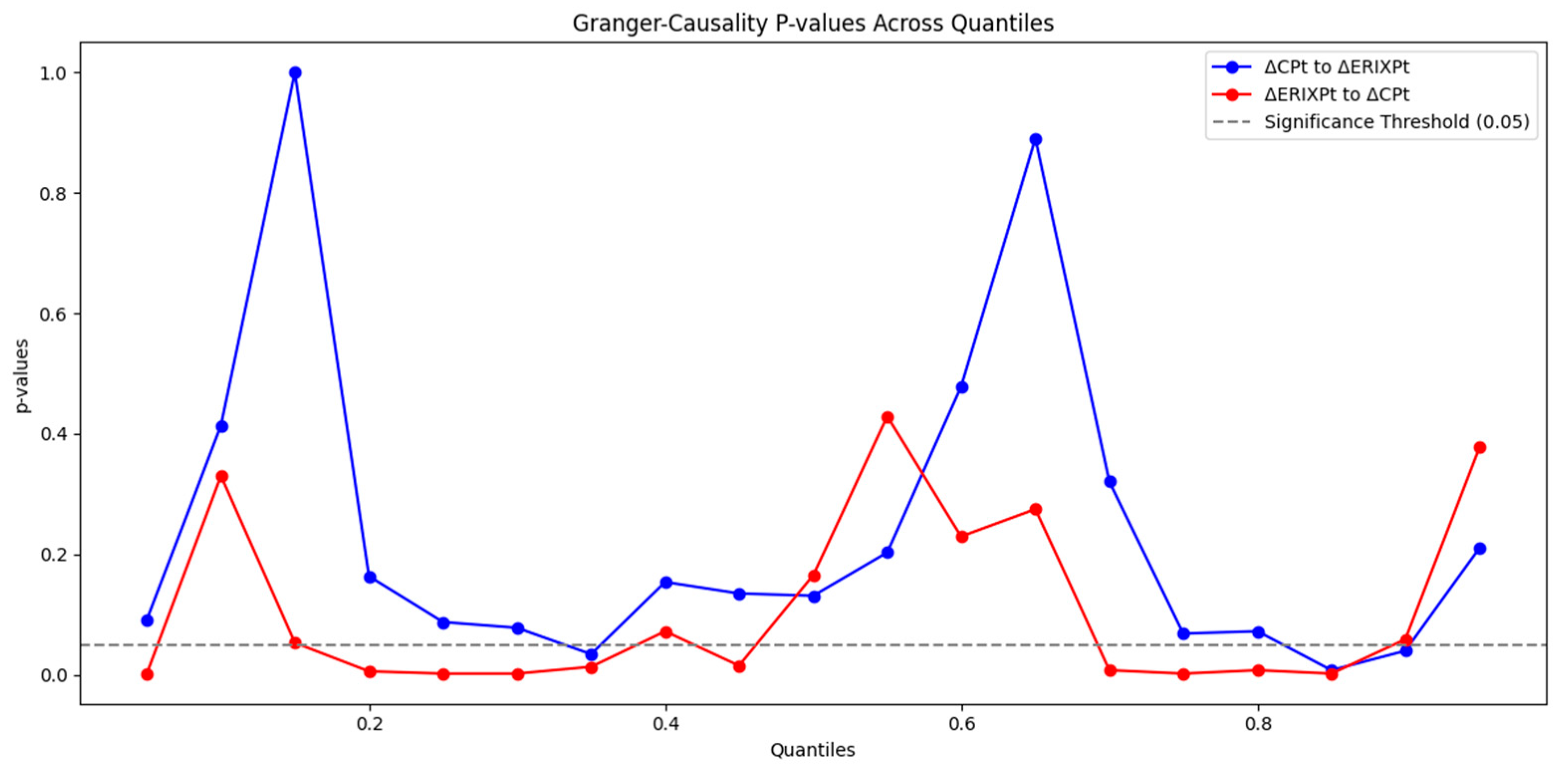
We additionally illustrate the p-values of the test for quantile Granger-causality between carbon and four clean energy indexes. Figure 3 illustrates the Granger-causality p-values across quantiles for the bidirectional link between ΔCPt and ΔERIXPt. The blue line denotes the p-values for assessing whether ΔCPt Granger-causes ΔERIXPt, whereas the red line signifies the p-values for the inverse causality. The dashed horizontal line at 0.05 indicates the standard significance threshold. Values below this level indicate statistically significant causation at the respective quantiles. The results indicate differences in causal influence at various quantile levels, suggesting possible nonlinear dynamics in the link between the two variables. Similarly, the unprecedented data indicate that nonlinear dynamics exist in the causal relationships between quantiles among CP, SPGCE, ECO, and CSINEI.
Moreover, following Troster et al. [57], we estimate the coefficient β τ in Equation (8) so that we can identify the causal relations between ΔCPt and all ΔSPGCEt, ΔERIXPt, ΔECOt, and ΔCSINEIt. The estimated value of coefficient β τ for each conditional quantile is presented in Table 3 and Table 4. To ensure brevity and readability, we only present the regression coefficients for the key quantiles τ = { 0.05 ,   0.25 ,   0.50 ,   0.75 ,   0.95 } in the main text. The estimates coefficients for all the 19 quantiles of the distribution are provided in the Appendix A.2.
Table 3 reports the signs of the causality from carbon prices to four clean energy indices (i.e., SPGCE, ERIXP, ECO, and CSINEI). Significantly, the results vary with the indices. For the tail causal relations from ΔCPt to ΔSPGCEt, ΔERIXPt or ΔERIXPt, the estimated coefficients are negative for all the equally spaced grid of 19 quantiles. Therefore, variations in carbon price returns negatively affect the variations in SPGCE, ERIXP or ECO. The results are counterintuitive and against our expectations. Generally, the rise in carbon prices directly affects the operating costs and profit models of businesses, thereby promoting the demand for clean energy and driving the performance of the clean energy industry. We argue that the negative effects of carbon prices on clean energy stock prices are most likely due to the comparative cost disadvantage and cost of production. About the former, positive fluctuations in carbon prices can make fossil fuel-based energy sources relatively more expensive compared to cleaner alternatives. However, on the one hand, clean energy technologies are still in various stages of development and deployment, and their costs remain relatively higher than traditional energy sources in some cases. On the other hand, in the short run, it is difficult for traditional companies to adjust their energy structure, which makes their demand for traditional energy sources inelastic. As a result, clean energy companies may face challenges in competing with fossil fuel-based companies that can pass on the increased cost burden to consumers. As for the latter, rising carbon prices impact the usage cost of other commodities, such as natural gas or coal, which are often required by clean energy companies to carry out production activities. Therefore, a rise in commodity prices can influence the profitability of clean energy companies and affect investor perceptions of their financial viability.
When focusing on the Granger-causality from ΔCPt to ΔCSINEIt, the estimated coefficients are positive for all the quantiles of the conditional distribution, which indicate that carbon price has a positive effect on CSINEI. Thus, sufficiently large carbon shocks positively affect the variations in CSINEI. The results conform to the expectations. As discussed already, rising carbon prices cause traditional energy sources to become more costly. By contrast, fewer or no carbon emissions are produced by clean energy sources such hydroelectric power, solar, and wind. As a result, their relative cost competitiveness rises, which boosts demand and drives higher stock prices for businesses engaged in clean energy generation.
Initially, policy frameworks, market dynamics, and the makeup of the energy sector in every location affect how variations in carbon prices affect the worldwide, European, U.S., and Chinese clean energy markets. One important consideration is China’s different approach to renewable energy policies and carbon pricing than those of industrialized nations. China has implemented a range of initiatives to support clean energy development, including ambitious renewable energy targets. The government’s strong commitment to clean energy has fostered a favorable policy environment, boosting investor confidence and generating positive market sentiment. In contrast, the United States has a more fragmented policy landscape, with varying levels of clean energy support at the federal and state levels. Inconsistent regulatory incentives and a lack of a single federal carbon pricing mechanism have reduced investor confidence in the U.S. clean energy sector. These variations in policy support systems and regulatory strategies help to explain why changes in the carbon price have diverse effects on clean energy stock values in various areas.
Second, the dynamics of renewable energy marketplaces in China, Europe, and the United States vary considerably, influencing the effects of carbon price variations on stock prices. The clean energy business in China has undergone swift growth, propelled by significant government investments, favorable regulatory frameworks, and a sizable domestic market. These considerations have drawn significant capital inflows, cultivating a vigorous and swiftly expanding market for clean energy equities. Conversely, although the renewable energy sector in the United States and Europe has had significant development, these markets are more developed and intensely competitive. Both in Europe and the United States, the renewable energy industries have a diverse range of well-known businesses and upstart companies, each showing varying degrees of financial stability. Therefore, the effect of carbon prices on clean energy stock performance in these markets is more complex since market reactions are much influenced by company-specific elements.
At last, the makeup of the energy sector differs greatly between China and Western nations, which shapes how carbon pricing affects markets for clean energy. China still mostly depends on coal for generation of electricity; hence, carbon pricing becomes more important in guiding the change towards greener energy sources. Investors expect a move towards renewable alternatives as growing carbon costs raise the cost of coal-based electricity; hence, driving more demand for clean energy equities. By comparison, coal plays quite a small role in the energy mix in the United States and the European Union; natural gas and renewable energy make up a larger share here. Consequently, as the shift toward lower-carbon energy sources is already more advanced and incorporated into market systems, the effect of carbon pricing on clean energy stock performance in these markets is rather less marked.
Table 4 reports the sign of the causality from four clean energy indices to carbon prices. In the following analysis, we focus on the signs of the Granger-causality of the tails of the distribution τ = { 0.25 ,   0.50 ,   0.75 } because the causality from ΔSPGCEt, ΔERIXPt, ΔECOt or ΔCSINEIt to ΔCPt are significant at 5% level over these three quantiles according to the S T test. From ΔSPGCEt to ΔCPt, the estimated coefficients are negative at the 25th percentiles, and positive for τ = { 0.50 ,   0.75 } (the estimate values are small, however). From ΔERIXPt to ΔCPt, the estimated coefficients are negative except for τ = 0.25 ; from ΔECOt to ΔCPt, the estimated coefficients are positive for all the five quantiles; from ΔCSINEIt to ΔCPt, the estimated coefficients are positive except for τ = 0.75 , but their values are small.
The empirical results show a direct causal link between carbon markets and clean energy stocks at the tails of the conditional distribution. However, at the median quantile of the distribution (in the periods of the low market volatility), our quantile-based causality analysis suggests that the causal influence of carbon prices on clean energy stocks is not significant. To be specific, our empirical results show that the signs of the Granger-causality running from carbon markets to clean energy stocks are country- or region-specific. There are negative effects of carbon markets on global, European and U.S. clean energy stock prices but positive effects of that on China clean energy stocks (SPGCE, ERIXP, ECO and CSINEI are global, European, US and China clean energy indices, respectively) under bullish or bearish market conditions. Therefore, we call on policymakers in different countries or regions to implement differentiated carbon and clean energy policies. However, we do not find clear signs of the causal relations from clean energy stocks to carbon prices. Our findings imply that the clean energy indices can act as the hedging assets of carbon when in bullish or bearish market conditions and can also act as diversifiers of carbon under normal market conditions.

4. Discussion

This study offers quantile-specific insights into the causal relationship between carbon markets and clean energy stocks, indicating that causality is most pronounced in the tails of the return distribution while remaining insignificant at the median. The findings indicate that variations in carbon prices have distinct effects across different regions, influenced by market volatility, policy structures, and carbon pricing systems. The results have major policy ramifications for stabilizing carbon markets and maximizing clean energy investment plans.

4.1. Market Volatility and Policy Stability

Different policy environments can affect carbon markets, clean energy markets, and the carbon–clean energy nexus. Differentiated carbon trading, financial incentives, and regulatory policies affect carbon prices, clean energy stocks, and the relationship between them by affecting the supply and demand structure of carbon allowances and clean energy, and investor behavior and sentiment [59]. Meanwhile, policy uncertainty has an impact on the spillover effects between financial markets. Higher policy uncertainty increases the risk spillover effects between markets, thus impacting the relationship between the carbon market and clean energy stocks [60].
Particularly during times of bullish and bearish trends, our results show that carbon price volatility negatively affects the performance of clean energy equities worldwide, including in European and U.S. markets. This is in line with earlier studies showing that notable changes in carbon pricing create investment uncertainty, which compromises long-term commitments to projects aimed at sustainable energy. Unlike China’s state-owned carbon pricing policies, Western markets operate under more market-driven carbon trading schemes such as the EU ETS and RGGI. Under these systems, price volatility results from imbalances in energy supply and demand, speculative trading, and regulatory changes. The noted volatility might limit the efficiency of carbon pricing in encouraging acceptance of sustainable energy sources.

4.2. State Intervention and Green Finance in China

The clean energy market in China shows a different dynamic whereby growing carbon prices improve the performance of clean energy assets. State-backed sustainability initiatives help to explain this since they shield companies from cost constraints and encourage long-term clean energy investment. Policies supporting waste-to-energy integration, targeted subsidies, and preferential financing help to highlight the favorable spill-over effects of carbon pricing on renewable energy [61,62].
Stabilizing clean energy investments and mitigating carbon price volatility in China while increasing investment uncertainty in developed countries depends critically on green finance [56]. China’s green financial instruments—including green bonds, carbon credit financing, and ESG investments—ensure long-term capital allocation to clean energy, so strengthening market resilience unlike in the United States and Europe, where companies depend on traditional financing structures sensitive to short-term carbon market shocks.
Policy uncertainty and ineffective carbon trading systems increase investment hazards in wealthy countries even more. By improving market transparency, lowering speculative distortions, and boosting investor confidence, blockchain-based carbon trading platforms—like the Shanghai Environment and Energy Exchange—offer a possible answer [63]. Real-time verification, distributed transaction records, and immutable trading data among other features serve to stabilize carbon prices, thereby supporting long-term clean energy investment [64].
The inadequate integration of green finance in Western markets could help to explain the detrimental effect of changes in carbon prices on the supply of renewable energy. Long-term green infrastructure funds, carbon credit-linked financial products, and strengthening ESG requirements could help to sustain robust clean energy investments and hence improve market stability.

4.3. Implications for Carbon Trading Mechanisms

Findings suggest that regional differences in carbon price effects reflect fundamental variations in carbon trading mechanisms. The EU ETS, despite its scope, continues to exhibit high price volatility, while China’s pilot carbon markets are evolving toward greater centralization.
To enhance market stability, policymakers should implement carbon price stabilization mechanisms to mitigate excessive fluctuations in carbon trading schemes. Establishing price corridors or market stability reserves can help regulate volatility and prevent abrupt market distortions. Additionally, stronger linkages between carbon markets and green finance instruments would provide a financial buffer against carbon price risks, fostering long-term investment confidence. On a global scale, strengthening cross-border carbon market integration, such as aligning the EU ETS with China’s national carbon market, could reduce market fragmentation and price shocks. For China, further refinement of cap-and-trade mechanisms would enhance carbon market efficiency and long-term price predictability, ensuring a more stable and effective transition toward a low-carbon economy.

4.4. Summary of Policy Implications

This study underscores the importance of region-specific carbon policies tailored to market structures, financial systems, and regulatory environments. In Western economies, stabilizing carbon markets is crucial to reducing investment uncertainty, while in China, state intervention should be leveraged to enhance the role of carbon pricing in clean energy financing. Additionally, refining carbon trading mechanisms to improve the alignment between global carbon pricing frameworks can facilitate market integration and stability. By incorporating quantile-based insights into policy design, governments and investors can develop more resilient and effective low-carbon financial strategies, accelerating the transition toward sustainable energy systems.
To further strengthen carbon pricing as a tool for clean energy expansion, China could expand sectoral carbon credit integration by incorporating circular economy practices, ensuring stable carbon pricing while stimulating clean energy growth. Additionally, enhancing green financial mechanisms, such as green bonds and carbon-linked investment instruments, would attract private capital into renewables, fostering a more robust clean energy market.

5. Conclusions

This study provides new insights into the dynamic relationship between carbon markets and clean energy stocks, emphasizing nonlinear dependencies and region-specific effects. By employing a quantile Granger-causality framework, we reveal that causal linkages are strongest in extreme market conditions, while remaining insignificant at the median. The findings underscore the critical role of market structures, policy interventions, and financial mechanisms in shaping the effectiveness of carbon pricing on clean energy investments. Beyond identifying causal dynamics, this study highlights key policy considerations. In Western markets, carbon price volatility introduces investment uncertainty, necessitating stabilization mechanisms to ensure a predictable policy environment. In contrast, China’s state-driven approach to green finance mitigates these risks, allowing carbon pricing to function as an investment signal rather than a cost burden. These distinctions emphasize the need for regionally tailored carbon and clean energy policies to promote sustainable energy transitions.
However, there are still some limitations of this study. First, this study does not consider the Granger-causality in quantiles between fossil energy, carbon, and clean energy markets, as the fluctuations in conventional energy prices have an impact on the carbon and clean energy markets. Second, we do not empirically investigate the effects of macroeconomic factors such as economic policy uncertainty and geopolitical risks on the carbon–clean energy nexus. Therefore, future research can be extended from the above two directions. Future research should explore additional macroeconomic factors influencing the carbon–clean energy nexus, such as economic policy uncertainty, interest rate policies, geopolitical risks, and energy transition commitments. Additionally, expanding the analysis to firm-level ESG data and sector-specific carbon pricing effects could further refine our understanding of how carbon markets drive investment behavior. Furthermore, integrating green financial innovations, such as blockchain-based carbon trading and sustainability-linked bonds, into empirical models could provide a more comprehensive assessment of financial instruments in stabilizing clean energy investment.
By deepening the understanding of quantile-specific and region-specific interactions, this study contributes to the broader literature on climate finance and sustainable investment strategies, offering valuable implications for investors, policymakers, and researchers navigating the evolving carbon market landscape.

Author Contributions

Conceptualization, W.J. and J.J.; methodology, J.J.; software, J.J.; validation, W.J., J.J. and S.C.-I.C.; formal analysis, J.J.; investigation, J.J.; resources, J.J.; data curation, J.J.; writing—original draft preparation, J.J.; writing—review and editing, S.C.-I.C.; visualization, S.C.-I.C.; supervision, W.J.; project administration, S.C.-I.C.; funding acquisition S.C.-I.C. All authors have read and agreed to the published version of the manuscript.

Funding

This research received no funding.

Institutional Review Board Statement

Not applicable.

Informed Consent Statement

Not applicable.

Data Availability Statement

Data supporting the findings in this study are available from the corresponding authors.

Acknowledgments

The authors are highly grateful to the experts and scholars who gave suggestions to help us improve the manuscript.

Conflicts of Interest

The authors declare no conflicts of interest.

Abbreviations

The following abbreviations are used in this manuscript:
CPEUA future prices
SPGCES&P Global Clean Energy Index
ERIXPEuropean Renewable Energy Index
ECOWilder Hill Clean Energy Index
CSINEICSI New Energy Index

Appendix A

Appendix A.1

Table A1. Granger-causality between CP and SPGCE: subsampling p-values.
τΔCPt to ΔSPGCEtΔSPGCEt to ΔCPt
I t Δ SPGCE t = 1 I t Δ SPGCE t = 2 I t Δ SPGCE t = 3 I t Δ CP t = 1   I t Δ CP t = 2   I t Δ CP t = 3
[0.05:0.95]0.006 ***0.002 ***0.004 ***0.002 ***0.002 ***0.002 ***
0.050.061 *0.1030.1030.3300.2960.380
0.100.004 ***0.002 ***0.002 ***0.053 *0.068 *0.021 **
0.150.002 ***0.002 ***0.002 ***0.006 ***0.078 *0.002 ***
0.200.004 ***0.002 ***0.002 ***0.002 ***0.002 ***0.015 **
0.250.023 **0.004 ***0.002 ***0.002 ***0.002 ***0.002 ***
0.300.027 **0.038 **0.021 **0.002 ***0.002 ***0.002 ***
0.350.036 **0.059 *0.061 *0.013 **0.004 ***0.002 ***
0.400.044 **0.029 **0.027 **0.0720.095 *0.049 **
0.450.1100.2260.1670.015 **0.002 ***0.019 **
0.500.2410.2140.3740.1650.2070.013 **
0.550.4710.2810.2520.4290.5050.269
0.600.1120.2410.1350.2300.1331.000
0.650.002 ***0.002 ***0.002 ***0.2750.3210.184
0.700.002 ***0.002 ***0.002 ***0.008 ***0.002 ***0.017 **
0.750.002 ***0.002 ***0.002 ***0.002 ***0.002 ***0.002 ***
0.800.002 ***0.002 ***0.002 ***0.008 ***0.002 ***0.002 ***
0.850.002 ***0.002 ***0.002 ***0.002 ***0.013 **0.011 **
0.900.010 ***0.053 *0.066 *0.059 *0.002 ***0.047 **
0.950.3400.6640.6320.3780.3530.302
This table reports the p-values of S T test for quantile Granger-causality between CP and SPGCE. ΔSPGCEt and ΔCPt represent the log-difference data (log return) of SPGCE and CP, respectively. I t Δ SPGCE t and I t Δ CP t are the lag lengths of ΔSPGCEt and ΔCPt, respectively, included in Equation (7). The size of the subsample is b = 64 and the number of observations is T = 593. ***, **, * denote the significance level at 1%, 5%, 10%, respectively.
Table A2. Granger-causality between CP and ERIXP: subsampling p-values.
τΔCPt to ΔERIXPtΔERIXPt to ΔCPt
I t Δ ERIXP t = 1   I t Δ ERIXP t = 2     I t Δ ERIXP t = 3 I t Δ CP t = 1 I t Δ CP t = 2   I t Δ CP t = 3
[0.05:0.95]0.091 *0.078 *0.059 *0.002 ***0.002 ***0.002 ***
0.050.4140.1290.1310.3300.2960.380
0.101.0001.0001.0000.053 *0.068 *0.021 **
0.150.1630.1460.1420.006 ***0.0780.002 ***
0.200.084 *0.080 **0.082 *0.002 ***0.002 ***0.015 **
0.250.087 *0.082 *0.076 *0.002 ***0.002 ***0.002 ***
0.300.078 *0.049 **0.021 **0.002 ***0.002 ***0.002 ***
0.350.034 **0.006 ***0.002 ***0.013 **0.004 ***0.002 ***
0.400.1540.1460.2470.072 *0.095 *0.049 **
0.450.1350.1180.082 *0.015 **0.002 ***0.019 **
0.500.1310.1330.087 *0.1650.2070.013 **
0.550.2030.2110.2030.4290.5050.269
0.600.4780.3740.3340.2300.1331.000
0.650.8900.6150.4920.2750.3210.184
0.700.3210.4180.3570.008 ***0.002 ***0.017 **
0.750.068 *0.049 **0.059 *0.002 ***0.002 ***0.002 ***
0.800.072 *0.061 *0.057 *0.008 ***0.002 ***0.002 ***
0.850.008 ***0.011 **0.004 ***0.002 ***0.013 **0.011 **
0.900.040 **0.1270.042 **0.059 *0.002 ***0.047 **
0.950.2110.1670.1500.3780.3530.302
This table reports the p-values of S T test for quantile Granger-causality between CP and ERIXP. ΔERIXPt and ΔCPt represent the log-difference data (log return) of ERIXP and CP, respectively. I t Δ ERIXP t and I t Δ CP t are the lag lengths of ΔERIXPt and ΔCPt, respectively, included in Equation (7). The size of the subsample is b = 64 and the number of observations is T = 593. The p-values in bold denote the 1% significance level. ***, **, * denote the significance level at 1%, 5%, 10%, respectively.
Table A3. Granger-causality between CP and ECO: subsampling p-values.
τΔCPt to ΔECOtΔECOt to ΔCPt
I t Δ ECO t = 1   I t Δ ECO t = 2 I t Δ ECO t = 3 I t Δ CP t = 1 I t Δ CP t = 2 I t Δ CP t = 3
[0.05:0.95]0.002 ***0.008 ***0.013 **0.002 ***0.002 ***0.002 ***
0.050.4270.3380.7700.3300.2960.380
0.100.1940.2880.011 **0.053 *0.068 *0.021 **
0.150.002 ***0.002 ***0.002 ***0.006 ***0.078 *0.002 ***
0.200.002 ***0.002 ***0.002 ***0.002 ***0.002 ***0.015 **
0.250.017 **0.023 **0.019 **0.002 ***0.002 ***0.002 ***
0.300.042 **0.047 **0.034 **0.002 ***0.002 ***0.002 ***
0.350.044 **0.027 **0.044 **0.013 **0.004 ***0.002 ***
0.400.099 *0.055 *0.093 *0.072 *0.095 *0.049 **
0.450.034 **0.082 *0.087 *0.015 **0.002 ***0.019 **
0.500.095 *0.2110.4180.1650.2070.013 **
0.550.8250.8540.8770.4290.5050.269
0.600.082 *0.1060.2180.2300.1330.998
0.650.002 ***0.051 *0.068 *0.2750.3210.184
0.700.002 ***0.002 ***0.004 ***0.008 ***0.002 ***0.017 **
0.750.002 ***0.002 ***0.002 ***0.002 ***0.002 ***0.002 ***
0.800.002 ***0.002 ***0.002 ***0.008 ***0.002 ***0.002 ***
0.850.002 ***0.002 ***0.002 ***0.002 ***0.013 **0.011 **
0.900.023 **0.038 **0.025 **0.059 *0.002 ***0.047 **
0.950.8050.8030.6960.3780.3530.306
This table reports the p-values of S T test for quantile Granger-causality between CP and ECO. ΔECOt and ΔCPt represent the log-difference data (log return) of ECO and CP, respectively. I t Δ ECO t and I t Δ CP t are the lag lengths of ΔECOt and ΔCPt, respectively, included in Equation (7). The size of the subsample is b = 64 and the number of observations is T = 593. The p-values in bold denote the 1% significance level. ***, **, * denote the significance level at 1%, 5%, 10%, respectively.
Table A4. Granger-causality between CP and CSINEI: subsampling p-values.
τΔCPt to ΔCSINEItΔCSINEIt to ΔCPt
I t Δ CSINEI t = 1   I t Δ CSINEI t = 2     I t Δ CSINEI t = 3 I t Δ CP t = 1 I t Δ CP t = 2   I t Δ CP t = 3
[0.05:0.95]0.010 ***0.008 ***0.011 **0.002 ***0.002 ***0.010 ***
0.050.2880.5900.6960.3300.3130.288
0.100.002 ***0.006 ***0.006 ***0.053 *0.068 *0.002 ***
0.150.042 **0.030 **0.021 **0.006 ***0.078 *0.042 **
0.200.066 *0.011 **0.011 **0.002 ***0.002 ***0.066 *
0.250.002 ***0.002 ***0.002 ***0.002 ***0.002 ***0.002 ***
0.300.002 ***0.002 ***0.002 ***0.002 ***0.002 ***0.002 ***
0.350.015 **0.051 *0.030 **0.013 ***0.004 ***0.015 **
0.400.030 **0.080 *0.063 *0.072 *0.09580.030 **
0.450.011 **0.059 **0.07480.015 **0.002 ***0.011 **
0.500.3210.010 ***0.1180.1650.2070.321
0.550.6410.6220.3620.4290.5050.641
0.600.7420.7910.6660.2300.1330.742
0.650.065 *0.008 ***0.040 *0.2750.3210.065 *
0.700.030 **0.029 **0.01080.008 ***0.002 ***0.030 **
0.750.036 **0.010 ***0.002 ***0.002 ***0.002 ***0.036 **
0.800.019 **0.011 **0.006 ***0.008 ***0.002 ***0.019 **
0.850.049 **0.032 **0.0530.002 ***0.013 **0.049 **
0.900.2790.2470.1010.059 *0.002 ***0.279
0.950.084 *0.2560.2030.3780.3530.084 *
This table reports the p-values of S T test for quantile Granger-causality between CP and CSINEI. ΔCSINEIt and ΔCPt represent the log-difference data (log return) of CSINEI and CP, respectively. I t Δ CSINEI t and I t Δ CP t are the lag lengths of ΔCSINEIt and ΔCPt, respectively, included in Equation (7). The size of the subsample is b = 64 and the number of observations is T = 593. The p-values in bold denote the 1% significance level. ***, **, * denote the significance level at 1%, 5%, 10%, respectively.

Appendix A.2

Table A5. Quantile regression estimated coefficients from carbon returns to clean energy index returns.
τΔCPt to ΔSPGCEtΔCPt to ΔERIXPtΔCPt to ΔECOtΔCPt to ΔCSINEIt
0.05−0.117−0.015−0.1760.051
0.10−0.072−0.075−0.1430.094
0.15−0.067−0.071−0.0980.062
0.20−0.058−0.062−0.0850.022
0.25−0.050−0.034−0.0390.021
0.30−0.035−0.055−0.0510.018
0.35−0.050−0.045−0.0660.030
0.40−0.041−0.051−0.0620.037
0.45−0.038−0.054−0.0560.025
0.50−0.037−0.062−0.0560.019
0.55−0.032−0.040−0.0540.016
0.60−0.046−0.059−0.0640.024
0.65−0.043−0.044−0.0750.010
0.70−0.049−0.050−0.0960.017
0.75−0.063−0.046−0.0990.018
0.80−0.065−0.027−0.0950.025
0.85−0.094−0.013−0.0810.044
0.90−0.111−0.025−0.0730.054
0.95−0.141−0.059−0.1380.034
This table reports the coefficients β τ across the 19 quantiles in Equation (8).
Table A6. Quantile regression estimated coefficients from clean energy index returns to carbon returns.
τΔSPGCEt to ΔCPtΔERIXPt to ΔCPtΔECOt to ΔCPtΔCSINEIt to ΔCPt
0.050.184−0.0010.2270.197
0.100.2700.1470.1860.134
0.150.1080.0020.1840.101
0.200.0600.0620.0730.059
0.25−0.0260.0220.0420.004
0.30−0.099−0.0090.047−0.026
0.35−0.056−0.0020.052−0.045
0.40−0.0530.058−0.005−0.005
0.45−0.0720.0250.0350.022
0.500.001−0.0230.0270.003
0.550.0400.0230.047−0.022
0.600.0820.0180.0810.001
0.650.0600.0050.083−0.046
0.70−0.011−0.0540.024−0.021
0.750.009−0.0070.009−0.065
0.80−0.029−0.033−0.039−0.055
0.850.0040.0400.010−0.109
0.90−0.0080.010−0.009−0.167
0.95−0.211−0.1160.029−0.234
This table reports the coefficients β τ across the 19 quantiles in Equation (8).

References

  1. Cachon, G.P. Retail store density and the cost of greenhouse gas emissions. Manag. Sci. 2014, 60, 1907–1925. [Google Scholar]
  2. Avci, B.; Girotra, K.; Netessine, S. Electric vehicles with a battery switching station: Adoption and environmental impact. Manag. Sci. 2015, 61, 772–794. [Google Scholar]
  3. Scott, A.; Li, M.; Cantor, D.E.; Corsi, T.M. Do voluntary environmental programs matter? Evidence from the EPA SmartWay program. J. Oper. Manag. 2023, 69, 284–304. [Google Scholar]
  4. İşlegen, Ö.; Reichelstein, S. Carbon capture by fossil fuel power plants: An economic analysis. Manag. Sci. 2011, 57, 21–39. [Google Scholar]
  5. Naumov, S.; Keith, D.R.; Sterman, J.D. Accelerating vehicle fleet turnover to achieve sustainable mobility goals. J. Oper. Manag. 2023, 69, 36–66. [Google Scholar]
  6. Dooley, K.J.; Pathak, S.D.; Kull, T.J.; Wu, Z.; Johnson, J.; Rabinovich, E. Process network modularity, commonality, and greenhouse gas emissions. J. Oper. Manag. 2019, 65, 93–113. [Google Scholar]
  7. Zhu, B.; Ye, S.; Han, D.; Wang, P.; He, K.; Wei, Y.-M.; Xie, R. A multiscale analysis for carbon price drivers. Energy Econ. 2019, 78, 202–216. [Google Scholar]
  8. Zhang, Y.-J.; Sun, Y.-F. The dynamic volatility spillover between European carbon trading market and fossil energy market. J. Clean. Prod. 2016, 112, 2654–2663. [Google Scholar]
  9. Wang, Y.; Guo, Z. The dynamic spillover between carbon and energy markets: New evidence. Energy 2018, 149, 24–33. [Google Scholar]
  10. Tan, X.-P.; Wang, X.-Y. Dependence changes between the carbon price and its fundamentals: A quantile regression approach. Appl. Energy 2017, 190, 306–325. [Google Scholar]
  11. Soliman, A.M.; Nasir, M.A. Association between the energy and emission prices: An analysis of EU emission trading system. Resour. Policy 2019, 61, 369–374. [Google Scholar]
  12. Hammoudeh, S.; Nguyen, D.K.; Sousa, R.M. Energy prices and CO2 emission allowance prices: A quantile regression approach. Energy Policy 2014, 70, 201–206. [Google Scholar]
  13. Hammoudeh, S.; Nguyen, D.K.; Sousa, R.M. What explain the short-term dynamics of the prices of CO2 emissions? Energy Econ. 2014, 46, 122–135. [Google Scholar]
  14. Duan, K.; Ren, X.; Shi, Y.; Mishra, T.; Yan, C. The marginal impacts of energy prices on carbon price variations: Evidence from a quantile-on-quantile approach. Energy Econ. 2021, 95, 105131. [Google Scholar]
  15. Chevallier, J.; Khuong Nguyen, D.; Carlos Reboredo, J. A conditional dependence approach to CO2-energy price relationships. Energy Econ. 2019, 81, 812–821. [Google Scholar]
  16. Chevallier, J. A model of carbon price interactions with macroeconomic and energy dynamics. Energy Econ. 2011, 33, 1295–1312. [Google Scholar]
  17. Batten, J.A.; Maddox, G.E.; Young, M.R. Does weather, or energy prices, affect carbon prices? Energy Econ. 2021, 96, 105016. [Google Scholar]
  18. Wen, F.; Zhao, L.; He, S.; Yang, G. Asymmetric relationship between carbon emission trading market and stock market: Evidences from China. Energy Econ. 2020, 91, 104850. [Google Scholar]
  19. Tian, Y.; Akimov, A.; Roca, E.; Wong, V. Does the carbon market help or hurt the stock price of electricity companies? Further evidence from the European context. J. Clean. Prod. 2016, 112, 1619–1626. [Google Scholar]
  20. Moreno, B.; Pereira da Silva, P. How do Spanish polluting sectors’ stock market returns react to European Union allowances prices? A panel data approach. Energy 2016, 103, 240–250. [Google Scholar]
  21. Luo, C.; Wu, D. Environment and economic risk: An analysis of carbon emission market and portfolio management. Environ. Res. 2016, 149, 297–301. [Google Scholar] [PubMed]
  22. Jiménez-Rodríguez, R. What happens to the relationship between EU allowances prices and stock market indices in Europe? Energy Econ. 2019, 81, 13–24. [Google Scholar]
  23. Ji, Q.; Xia, T.; Liu, F.; Xu, J.-H. The information spillover between carbon price and power sector returns: Evidence from the major European electricity companies. J. Clean. Prod. 2019, 208, 1178–1187. [Google Scholar]
  24. Jong, T.; Couwenberg, O.; Woerdman, E. Does EU emissions trading bite? An event study. Energy Policy 2014, 69, 510–519. [Google Scholar]
  25. Fang, S.; Lu, X.; Li, J.; Qu, L. Multifractal detrended cross-correlation analysis of carbon emission allowance and stock returns. Phys. A Stat. Mech. Its Appl. 2018, 509, 551–566. [Google Scholar]
  26. da Silva, P.P.; Moreno, B.; Figueiredo, N.C. Firm-specific impacts of CO2 prices on the stock market value of the Spanish power industry. Energy Policy 2016, 94, 492–501. [Google Scholar]
  27. Aatola, P.; Ollikainen, M.; Toppinen, A. Price determination in the EU ETS market: Theory and econometric analysis with market fundamentals. Energy Econ. 2013, 36, 380–395. [Google Scholar]
  28. Jiang, W.; Liu, Y.; Xue, W. How do fossil energy markets and carbon markets affect each other? Based on the grainger causal relationship on quantiles. J. Clean. Prod. 2023, 423, 138799. [Google Scholar]
  29. Reboredo, J.C.; Ugolini, A. The impact of energy prices on clean energy stock prices. A Multivar. Quantile Depend. Approach. Energy Econ. 2018, 76, 136–152. [Google Scholar]
  30. Sun, C.; Ding, D.; Fang, X.; Zhang, H.; Li, J. How do fossil energy prices affect the stock prices of new energy companies? Evidence from Divisia energy price index in China’s market. Energy 2019, 169, 637–645. [Google Scholar]
  31. Umar, M.; Farid, S.; Naeem, M.A. Time-frequency connectedness among clean-energy stocks and fossil fuel markets: Comparison between financial, oil and pandemic crisis. Energy 2022, 240, 122702. [Google Scholar]
  32. Wu, Q.; Wang, M.; Tian, L. The market-linkage of the volatility spillover between traditional energy price and carbon price on the realization of carbon value of emission reduction behavior. J. Clean. Prod. 2020, 245, 118682. [Google Scholar]
  33. Xia, T.; Ji, Q.; Zhang, D.; Han, J. Asymmetric and extreme influence of energy price changes on renewable energy stock performance. J. Clean. Prod. 2019, 241, 118338. [Google Scholar]
  34. Ahmad, W. On the dynamic dependence and investment performance of crude oil and clean energy stocks. Res. Int. Bus. Financ. 2017, 42, 376–389. [Google Scholar]
  35. Bondia, R.; Ghosh, S.; Kanjilal, K. International crude oil prices and the stock prices of clean energy and technology companies: Evidence from non-linear cointegration tests with unknown structural breaks. Energy 2016, 101, 558–565. [Google Scholar]
  36. Dawar, I.; Dutta, A.; Bouri, E.; Saeed, T. Crude oil prices and clean energy stock indices: Lagged and asymmetric effects with quantile regression. Renew. Energy 2021, 163, 288–299. [Google Scholar]
  37. Ferrer, R.; Shahzad, S.J.H.; López, R.; Jareño, F. Time and frequency dynamics of connectedness between renewable energy stocks and crude oil prices. Energy Econ. 2018, 76, 1–20. [Google Scholar]
  38. Kocaarslan, B.; Soytas, U. Asymmetric pass-through between oil prices and the stock prices of clean energy firms: New evidence from a nonlinear analysis. Energy Rep. 2019, 5, 117–125. [Google Scholar]
  39. Paiva, A.S.S.; Rivera-Castro, M.A.; Andrade, R.F.S. DCCA analysis of renewable and conventional energy prices. Phys. A Stat. Mech. Its Appl. 2018, 490, 1408–1414. [Google Scholar]
  40. Reboredo, J.C. Is there dependence and systemic risk between oil and renewable energy stock prices? Energy Econ. 2015, 48, 32–45. [Google Scholar]
  41. Reboredo, J.C.; Rivera-Castro, M.A.; Ugolini, A. Wavelet-based test of co-movement and causality between oil and renewable energy stock prices. Energy Econ. 2017, 61, 241–252. [Google Scholar]
  42. Sadorsky, P. Correlations and volatility spillovers between oil prices and the stock prices of clean energy and technology companies. Energy Econ. 2012, 34, 248–255. [Google Scholar]
  43. Kumar, S.; Managi, S.; Matsuda, A. Stock prices of clean energy firms, oil and carbon markets: A vector autoregressive analysis. Energy Econ. 2012, 34, 215–226. [Google Scholar]
  44. Dutta, A. Oil price uncertainty and clean energy stock returns: New evidence from crude oil volatility index. J. Clean. Prod. 2017, 164, 1157–1166. [Google Scholar]
  45. Dutta, A.; Bouri, E.; Noor, M.H. Return and volatility linkages between CO2 emission and clean energy stock prices. Energy 2018, 164, 803–810. [Google Scholar]
  46. Hanif, W.; Arreola Hernandez, J.; Mensi, W.; Kang, S.H.; Uddin, G.S.; Yoon, S.-M. Nonlinear dependence and connectedness between clean/renewable energy sector equity and European emission allowance prices. Energy Econ. 2021, 101, 105409. [Google Scholar]
  47. Tiwari, A.K.; Aikins Abakah, E.J.; Gabauer, D.; Dwumfour, R.A. Dynamic spillover effects among green bond, renewable energy stocks and carbon markets during COVID-19 pandemic: Implications for hedging and investments strategies. Glob. Financ. J. 2022, 51, 100692. [Google Scholar]
  48. Wang, X.; Li, J.Y.; Ren, X.H. Asymmetric causality of economic policy uncertainty and oil volatility index on time-varying nexus of the clean energy, carbon and green bond. Int. Rev. Financ. Anal. 2022, 83, 102306. [Google Scholar]
  49. Mo, B.; Li, Z.; Meng, J. The dynamics of carbon on green energy equity investment: Quantile-on-quantile and quantile coherency approaches. Environ. Sci. Pollut. Res. Int. 2022, 29, 5912–5922. [Google Scholar]
  50. Troster, V. Testing for Granger-causality in quantiles. Econom. Rev. 2016, 37, 850–866. [Google Scholar]
  51. Chuang, C.-C.; Kuan, C.-M.; Lin, H.-Y. Causality in quantiles and dynamic stock return–volume relations. J. Bank. Financ. 2009, 33, 1351–1360. [Google Scholar] [CrossRef]
  52. Koenker, R.; Machado, J.A.F. Goodness of fit and related inference processes for quantile regression. J. Am. Stat. Assoc. 1999, 94, 1296–1310. [Google Scholar] [CrossRef]
  53. Hong, Y.; Liu, Y.; Wang, S. Granger causality in risk and detection of extreme risk spillover between financial markets. J. Econom. 2009, 150, 271–287. [Google Scholar] [CrossRef]
  54. Balcilar, M.; Gupta, R.; Pierdzioch, C. Does uncertainty move the gold price? New evidence from a nonparametric causality-in-quantiles test. Resour. Policy 2016, 49, 74–80. [Google Scholar] [CrossRef]
  55. IEA. World Energy Investment; International Energy Agency: Paris, France, 2022. Available online: https://www.iea.org/reports/world-energy-investment-2022 (accessed on 1 December 2024).
  56. Chen, S.C.-I.; Xu, X.; Own, C.-M. The Impact of Green Finance and Technological Innovation on Corporate Environmental Performance: Driving Sustainable Energy Transitions. Energies 2024, 17, 5959. [Google Scholar] [CrossRef]
  57. Troster, V.; Shahbaz, M.; Uddin, G.S. Renewable energy, oil prices, and economic activity: A Granger-causality in quantiles analysis. Energy Econ. 2018, 70, 440–452. [Google Scholar] [CrossRef]
  58. Jarque, C.M.; Bera, A.K. Efficient tests for normality, homoscedasticity and serial independence of regression residuals. Econ. Lett. 1980, 6, 255–259. [Google Scholar]
  59. Ahmed, W.M.A.; Sleem, M.A.E. Short-and long-run determinants of the price behavior of US clean energy stocks: A dynamic ARDL simulations approach. Energy Econ. 2023, 124, 106771. [Google Scholar] [CrossRef]
  60. Ren, Y.; Tan, A.; Zhu, H.; Zhao, W. Does economic policy uncertainty drive nonlinear risk spillover in the commodity futures market? Int. Rev. Financ. Anal. 2022, 81, 102084. [Google Scholar] [CrossRef]
  61. Chen, S.C.-I.; Dang, X.; Xu, Q.-q.; Own, C.-M. Transforming Waste into Value: Sustainable Recycling of Agricultural Resources Under the ‘Carbon Peak and Carbon Neutrality’ Vision. Sustainability 2025, 17, 55. [Google Scholar] [CrossRef]
  62. Kumar, P.; Raj, A.; Kumar, V.A. Approach to Reduce Agricultural Waste via Sustainable Agricultural Practices. In Valorization of Biomass Wastes for Environmental Sustainability: Green Practices for the Rural Circular Economy; Springer Nature: Cham, Switzerland, 2024; pp. 21–50. [Google Scholar]
  63. Zhang, G.; Chen, S.C.-I.; Yue, X. Blockchain Technology in Carbon Trading Markets: Impacts, Benefits, and Challenges—A Case Study of the Shanghai Environment and Energy Exchange. Energies 2024, 17, 3296. [Google Scholar] [CrossRef]
  64. Abiodun, T.P.; Nnamdi, N.; Peter, O. Application of Blockchain Technology in Carbon Trading Market: A Systematic Review. IEEE Access 2024, 13, 5446–5470. [Google Scholar]
Figure 1. Research framework.
Sustainability 17 03118 g001
Figure 2. Prices and returns of EUA and four clean energy indices.
Sustainability 17 03118 g002
Figure 3. Quantile Granger-causality test: p-values across quantiles.
Sustainability 17 03118 g003
Table 1. Descriptive statistics.
ΔCPtΔSPGCEtΔERIXPtΔECOtΔCSINEIt
Mean0.0040.0010.0030.0010.002
Median0.0070.0020.0060.0030.004
Minimum−0.413−0.247−0.228−0.267−0.208
Maximum0.2320.1660.1160.1690107
Std. Dev.0.0700.0370.0360.0480.041
Skewness−0.858−0.381−0.638−0.295−0.625
Kurtosis7.3818.0505.9955.4995.246
Jarque-Bera546.151 ***643.240 ***261.464 ***162.669 ***163.032 ***
ADF Test−18.181 ***−14.961 ***−16.909 ***−15.364 ***−15.037 ***
*** denotes the significance level at 1%.
Table 2. Granger-causality between carbon and clean energy: subsampling p-values.
0.050.250.500.750.95
Panel A Granger-causality to clean energy indices
ΔCPt to ΔSPGCEt0.1030.002 ***0.3740.002 ***0.632
ΔCPt to ΔERIXPt0.1310.076 *0.087 *0.059 *0.150
ΔCPt to ΔECOt0.7700.019 **0.4180.002 ***0.025 **
ΔCPt to ΔCSINEIt0.6960.002 ***0.1180.002 ***0.203
Panel B Granger-causality to carbon prices
ΔSPGCEt to ΔCPt0.3800.002 ***0.013 **0.002 ***0.302
ΔERIXPt to ΔCPt0.3800.002 ***0.013 **0.002 ***0.302
ΔERIXPt to ΔCPt0.3800.002 ***0.013 **0.002 ***0.306
ΔCSINEIt to ΔCPt0.3800.002 ***0.013 **0.002 ***0.306
***, **, * denote the significance level at 1%, 5%, 10%, respectively.
Table 3. Quantile regression coefficients of carbon returns on clean energy returns.
τΔCPt to ΔSPGCEtΔCPt to ΔERIXPtΔCPt to ΔECOtΔCPt to ΔCSINEIt
0.05−0.117−0.015−0.1760.051
0.25−0.050−0.034−0.0390.021
0.50−0.037−0.062−0.0560.019
0.75−0.063−0.046−0.0990.018
0.95−0.141−0.059−0.1380.034
Table 4. Quantile regression coefficients of clean energy returns on carbon returns.
τΔSPGCEt to ΔCPtΔERIXPt to ΔCPtΔECOt to ΔCPtΔCSINEIt to ΔCPt
0.050.184−0.0010.2270.197
0.25−0.0260.0220.0420.004
0.500.001−0.0230.0270.003
0.750.009−0.0070.009−0.065
0.95−0.211−0.1160.029−0.234
Disclaimer/Publisher’s Note: The statements, opinions and data contained in all publications are solely those of the individual author(s) and contributor(s) and not of MDPI and/or the editor(s). MDPI and/or the editor(s) disclaim responsibility for any injury to people or property resulting from any ideas, methods, instructions or products referred to in the content.

