Article

Exploring the Performance and Interpretability of an Enhanced Data-Driven Model to Assess Surface Flooding Susceptibility

1
School of Natural Resources, Faculty of Geographical Science, Beijing Normal University, Beijing 100875, China
2
State Key Laboratory of Earth Surface Processes and Resource Ecology, Faculty of Geographical Science, Beijing Normal University, Beijing 100875, China
3
College of Water Sciences, Beijing Normal University, Beijing 100875, China
4
China Institute of Water Resources and Hydropower Research, Beijing 100038, China
*
Author to whom correspondence should be addressed.
Sustainability 2025, 17(7), 3065; https://doi.org/10.3390/su17073065
Submission received: 13 February 2025 / Revised: 27 March 2025 / Accepted: 28 March 2025 / Published: 30 March 2025
(This article belongs to the Section Sustainable Urban and Rural Development)

Abstract

:
The effects of climate change and increasing urbanization mean that urban areas are facing a greater risk of serious flooding. The paper aimed to adopt a data-driven approach to capture surface flood-prone features, providing a basis for surface flood susceptibility. This research developed an enhanced framework En-XGBoost, which consists of three modules: the core module, preprocessing module, and postprocessing module. Data augmentation, random extraction strategies, and local enhancement were introduced to improve the model’s performance. En-XGBoost was tested in Fuzhou, China. The main findings were as follows: (1) Neighborhood information extraction strategy outperformed information extraction strategy in extracting detailed flood-prone features, producing clearer boundaries between different flood susceptibility levels, and refining the flood risk areas. (2) Crucial explanatory variables were identified as major drivers of flood risk, with location-specific factors influencing the flood causes, necessitating localized analysis for specific sites. (3) The local enhancement, data augmentation, and random strategies improved model performance, with data augmentation proving more effective for stronger models and having limited impact on weaker ones. Model performance requires an appropriate alignment between data complexity and model complexity. En-XGBoost provided support for capturing surface flood-prone features.

1. Introduction

Under the influence of climate change and rapid urbanization, urban flooding has emerged as one of the most devastating natural disasters [1,2,3]. Globally, urban flooding causes significant economic losses and profound social disruptions [4], ranking among the most concerning natural hazards for human society [5,6]. It disrupts critical infrastructure such as communication, power, and transportation systems [7]. The expansion of urban construction and the proliferation of impervious surfaces have altered local hydrological characteristics, modified natural drainage pathways, and diminished infiltration and water retention capacities [8]. Together, these factors exacerbate runoff generation and significantly elevate flood risk [9]. Given the rising challenges posed by urban flooding, it is imperative to develop robust simulation and forecasting tools to support informed decision-making and effective flood management [9,10].
Physically-based models (PBMs) developed using hydrological and hydrodynamic methods [11], are widely employed for urban flood simulations [12,13,14,15]. By decomposing complex flood processes into hydrological, hydrodynamic, and their coupling processes, we can numerically solve these systems of partial differential equations using finite volume and finite element methods [16,17]. However, PBMs face significant limitations when applied to real-world urban-scale scenarios. Despite the maturity of numerical methods, urban-scale modeling still presents challenges such as large computational domains, extensive data requirements, and high consumption of computational resources, especially for high-resolution numerical algorithms [18,19]. For coastal urban areas in particular, achieving high model precision and computational efficiency is crucial [20]. Due to the compound disaster-causing factors driven by multiple flood sources, real-time computational demands for models become even more stringent. Addressing these challenges requires advancements that balance accuracy, efficiency, and scalability for urban-scale and coastal-specific flood modeling.
Data-driven models provide an alternative quantitative paradigm for representing surface flooding [21,22,23,24], which has increasingly been used for recognizing and detecting urban flood-prone locations [25]. Data-driven approaches typically build a surrogate model to fit the nonlinear relationships between feature variables and targets. Support vector machine [26], random forest [27], artificial neural network [28], and convolutional neural network [29] approaches have all been proposed. Machine learning methods establish mappings between input features and target states by integrating local environmental information and historical data, enabling the prediction of future flood inundation under similar conditions [26,30,31,32]. Indeed, although data-driven approaches require substantial time for model training and parameter learning, the learning process and the prediction process are relatively independent. This distinguishes them significantly from PBMs, where model improvements often demand considerable computational costs and resources that directly impact their application in new scenarios. In contrast, the independence of these processes in data-driven models ensures that the cost of model enhancement does not affect their usability in previously unseen contexts.
In modeling flood-prone areas in local surface regions using data-driven methods, PBMs can provide essential support for training datasets. A limitation of existing studies is the regularized nature of feature extraction for flood-prone areas, where the abstracted features often lack sufficient variation. Additionally, environmental feature extraction processes have not adequately incorporated randomness and uncertainty. However, when constructing flood-prone models that map urban attributes to specific local locations, introducing randomness and uncertainty has the potential to enhance the model’s generalization. Furthermore, the feature vectors captured during this process do not necessarily need to be regularized. To address these limitations, the current study adopts an integrated framework combining PBM and data-driven models to incorporate extensive stochastic strategies into nonlinear mapping and feature extraction. This approach enhances the model’s generalization and robustness while providing interpretability for the key factors influencing flood-prone areas. The primary contributions of this study are summarized as follows:
(1)
A framework En-XGBoost was constructed to achieve flood susceptibility mapping in urban scale, data-driven models inside En-XGBoost were compared to each other, and the indices of the model were evaluated.
(2)
Different feature extraction approaches were compared, and several groups of receptive fields were used to recognize the optimal neighborhood range. The flood susceptibility distributions were simulated, and the risk maps were implemented at multiple resolutions.
(3)
The crucial driving factors were provided, and the importances of explanatory features were evaluated. Subsequently, we conducted a detailed analysis of the interpretability of En-XGBoost in relation to flood susceptibility.
(4)
Several concepts were introduced and discussed, primarily including random strategies, local enhancement strategies, and data augmentation strategies. These ideas were incorporated into En-XGBoost. This research provides a detailed discussion of the combined benefits of these strategies, parameters, and their combinations.
This paper enhances the robustness of feature extraction by combining different feature extraction strategies, providing a reference for applying machine learning and data-driven methods in the study of surface flood susceptibility mapping.

2. Material and Methodology

An enhanced framework En-XGBoost for pluvial flood susceptibility mapping at the urban scale was developed. En-XGBoost integrates the ensemble learning model and SHAP method, coupling data augmentation, improved feature extraction, and an interpretable approach. The implementation procedure is shown in Figure 1. We adopted En-XGBoost to construct the nonlinear mapping from urban features to flood susceptibility, capturing the neighborhood information, and achieve the interpretation through SHAP method.

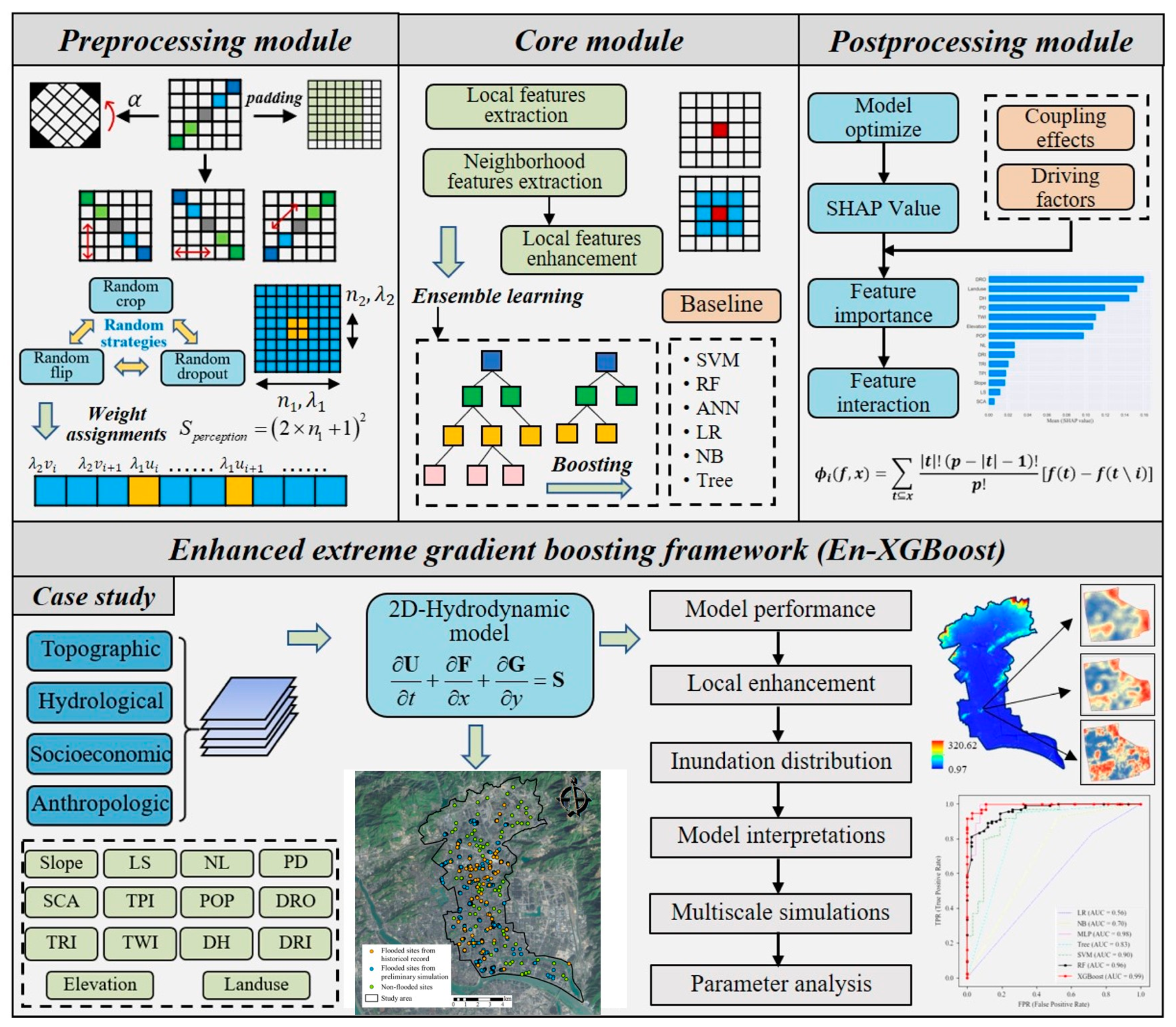
2.1. Modules Description in En-XGBoost

This research presented a novel data-driven framework, En-XGBoost, which enhances features mining through data augmentation and an interpretable system for modeling details. Based on traditional data-driven approaches, this framework primarily consists of three modules: the core module, the preprocessing module, and the postprocessing module. Additionally, there are two auxiliary modules: the hydrodynamic module and the baseline module.

2.1.1. Core Module

Ensemble learning combines multiple weak learners into a single, high-performance model [33,34]. XGBoost is an excellent ensemble learning method [35] presented by Chen and Guestrin [36]. The model takes several decision trees as the base classifier, while the input sample of the decision tree is related to the training and prediction results of the previous tree [37]. XGBoost introduces a regularization term in the objective function and updates the base learner according to the first-order and second-order derivatives in the iterations, making XGBoost more robust than the Gradient Boosting Decision Tree (GBDT) algorithm. During the model training process, the prediction function is derived based on the loss function, and the prediction function is updated at each iteration. The flowchart of the core model is shown in Figure 2.
Based on n trained trees, the prediction ( y ^ i ) of i-th sample and the objective function can be expressed as follows:
y ^ i = Σ k = 1 K f k x i ,   f k F
O b j = Σ i = 1 n l y i , y ^ i + Σ k = 1 K Ω f k
where x i is the i-th sample, fk is the prediction function of the n-th tree, K is the number of decision trees, F denotes all the tree functions, O b j represents the objective function, composed of the loss function and the complexity item.
Through transforming, optimizing O b j is equivalent to minimizing the object O b j k in training k-th tree. The expression can be further simplified using Taylor’s formula:
O b j k = i = 1 n   l [ y i , y ^ i ( t 1 ) + f t x i ] + Ω f k
O b j k = i = 1 n   l y i , y ^ i ( k 1 ) + g i f k x i + 1 2 h i f k 2 x i + Ω f k
g i = y ^ i ( k 1 ) l y i , y ^ i ( k 1 )
h i = y ^ i ( k 1 ) 2 l y i , y ^ i ( k 1 )
where g i and h i are respectively the first-order and second-order derivatives of the prediction function, which are constant terms when training the n-th tree.
Parameterizing the unknown in the formula, minimizing O b j k is equivalent to minimizing S k . Then, the greedy algorithm was used to optimize the structure of the trees:
S k = j = 1 T   i I j   g i ω j + 1 2 i I j   h i + λ ω j 2 + γ T
where γ is the complexity of the model, T is the number of leaves on the tree, λ is a constant, and ω j is the weight vectors.

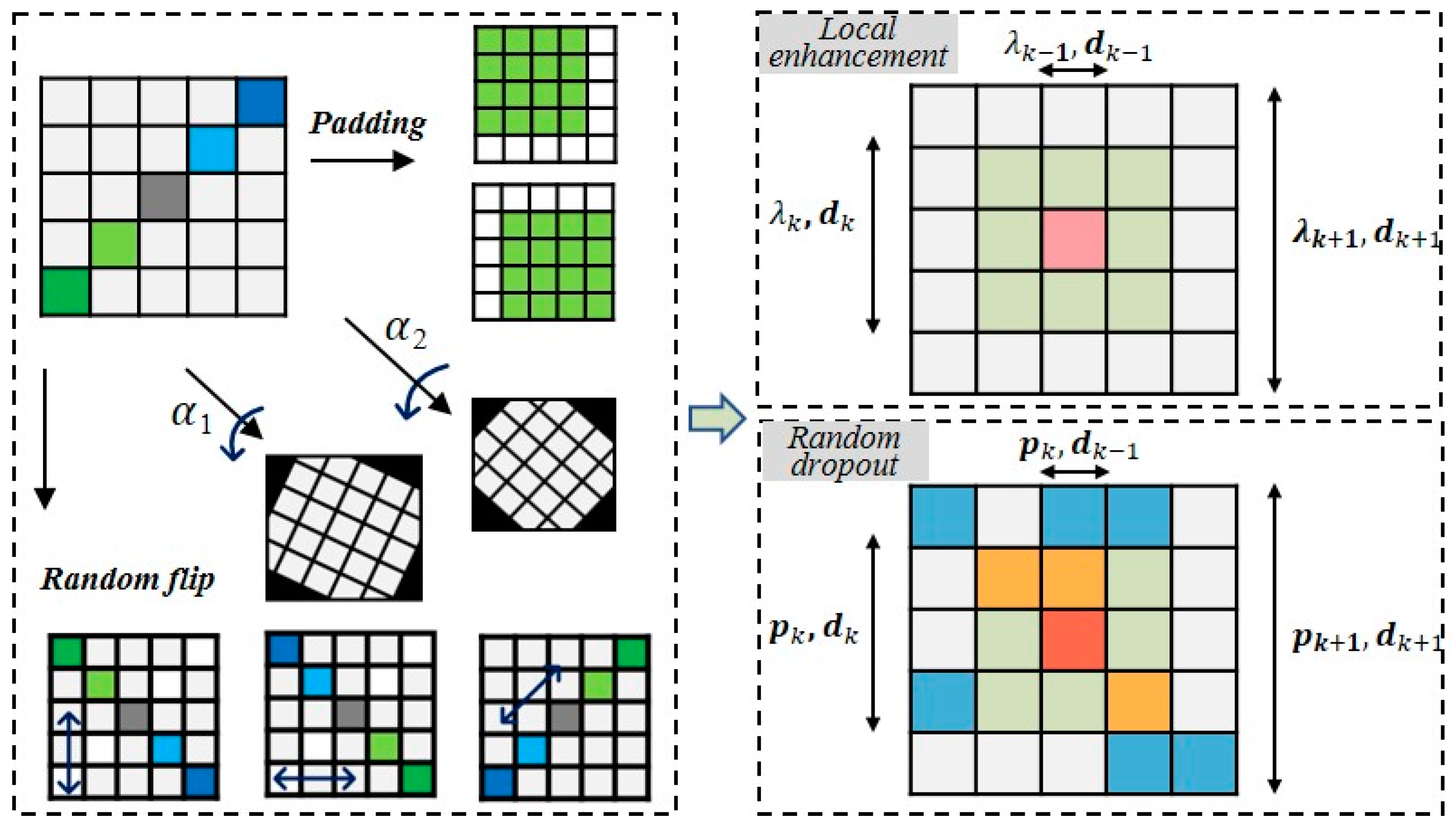
2.1.2. Preprocessing Module

The preprocessing module was developed to achieve effective feature extraction. Input strategies, data augmentation, and random strategies were incorporated into the module (Figure 3).
Two input strategies and several random feature extraction strategies were developed. The two input strategies were designed to capture local information. Strategy (a) uses local information as the input directly, the inputs are the features at each point, from which the state of the sites is obtained via the transformer. Strategy (b) uses neighborhood information as the input. A rectangular neighborhood window around the characteristic point is intercepted as the perceptual field of the local point. The elements within the window must be transformed into a feature vector before training. However, different perceptual ranges generate different simulation results. When a more extensive perceptual range is used, more domain information is incorporated, but if there is too much information in the neighborhood, it weakens the local information. Conversely, a smaller perceptual range might not adequately consider the domain information. Therefore, it is necessary to find an appropriate perceptual range to construct and optimize the model using the neighborhood range of perception centered on the local location as a variable, with the simulation effect as the goal. The range size was determined as follows:
S p = 2 × c + 1 2
where Sp (m2) denotes the perception range area, and c (m) denotes the perception range size.
Based on strategy (b), several random strategies were adopted during each feature extraction process. First, flip the original raster vertically, horizontally, or transpose it randomly. Second, pad the original raster and crop randomly. Third, rotate the original raster at a random angle. The module expands the samples, where the accompanying random strategy increases the randomness of the training samples and further strengthens the model’s generalization ability.
The information closer to the target point has a greater impact on determining the flooding state of the target point. Indeed, spatial features have local topological connections. However, such spatial relationships are lost in the process of feature representation. Thus, a regional weight distribution strategy (RWD) was introduced into the preprocessing module. We divide the regions near the points of interest into subregions according to the distances from the central point and assign weight factors (λk) accordingly to represent the importance of different regions. The raster value process was updated in Eq. 8:
H ( i , j ) = λ k h ( i , j ) , k = 1 , 2 , 3
where H ( i , j ) and h ( i , j ) are respectively the updated and original value in cell ( i , j ) , λ k represents the weighing factors of k-th subarea, d k represents the distance range of the k-th subarea.
Additionally, a random dropout strategy (RD) was introduced into the preprocessing module. Specifically, based on the previous subregions, we extract feature vectors by discarding a portion of the raster values in each subregion at different proportions. As a result, the feature vectors learned are primarily composed of features from spatial locations closer to the target site. This random strategy further increases the randomness in feature extraction, which in turn increases the generalization ability of the model. The random strategies and local enhancement were shown in Figure 4. Here, the parameter pk represents the probability to dropout in k-th subarea.

2.1.3. Postprocessing Module

The lack of interpretability has led to doubt regarding the reported outcomes [38]. Here, the driving factors and interpretations of the prediction are discussed based on the Shapely Additive explanations (SHAP) framework to analyze the primary factors forcing the flood-prone sites, and to identify the inundation response to the driving factors on an urban catchment scale. To understand the model calculations and predictions, SHAP values were used to break down the components of individual explanatory variables, thereby decomposing any prediction into the sum of the effects of each feature.
This approach has been proven effective in social fields [39,40]. Environmental features are considered contributors to the inundation state, based on SHAP, which is inspired by cooperative game theory. By breaking down the original black-box model, SHAP reveals the influence of each feature on the characteristics of each sample, showing both positive and negative effects [41]. By calculating the average marginal impact of the factors on the predicted value, SHAP assigns the expected significant value to each feature, providing a basis for the calculation of the interaction effect.
The shape values quantify the contributions to the prediction. For feature x j , the SHAP value ϕ i ( f , x ) is given by:
ϕ i ( f , x ) = t x   | t | ! ( p | t | 1 ) ! p ! [ f ( t ) f ( t \ i ) ]
where f represents the model; x is the set of possible combinations excluding x j ; p is the number of all features, | t | is all possible combinations of features.

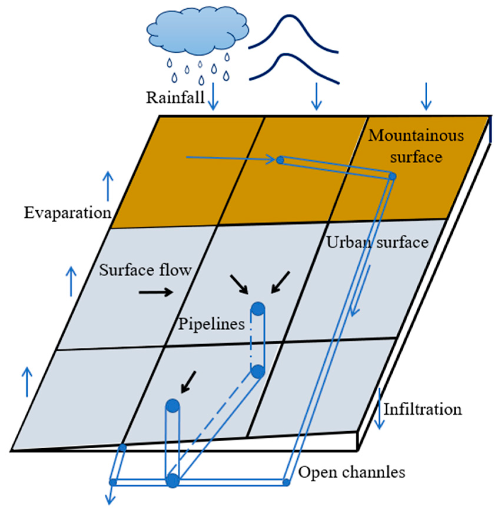
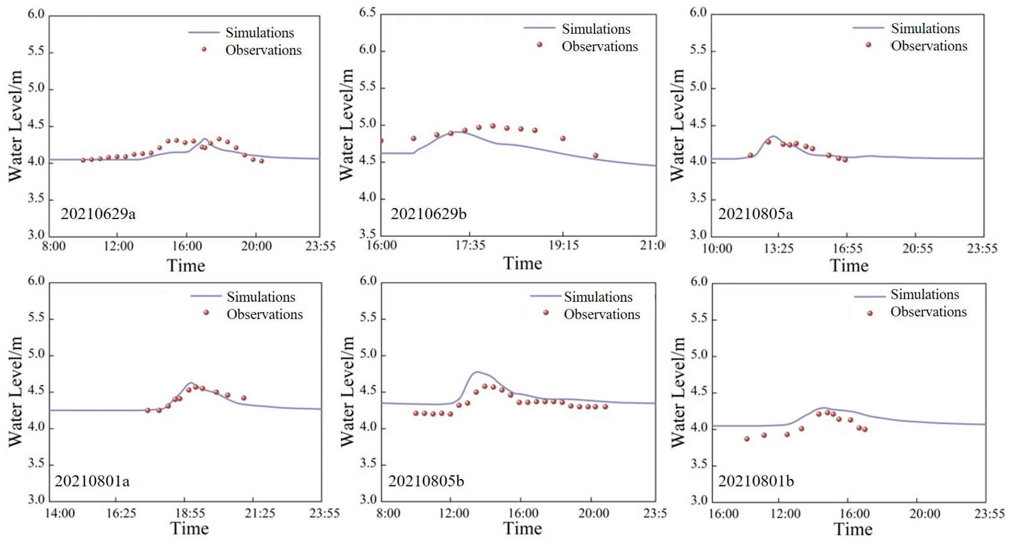
2.1.4. Hydrodynamic Module

The coupled hydrological and hydrodynamic model simulates multiple physical processes related to pluvial flooding, including mountainous runoff, drainage network flow, surface channel flow, and surface flooding flow. The entire process of urban pluvial flooding, from precipitation to surface inundation, is illustrated in Figure 5. The hydrodynamic module acts as an auxiliary component in En-XGBoost, enriching the data-driven model by supplementing it with flood-prone areas derived from mechanistic simulations.
Since the flood overflow process presents two-dimensional (2D) characteristics distinctly, the vertical acceleration of the water flow is generally ignored. The shallow water equations (SWE) are commonly used to model 2D flow in urban flood simulations [18,42]. SWE primarily represent horizontal flow dynamics, with minimal consideration of vertical flow components. The conserved form of the shallow water equations is represented as follows:
U t + F x + G y = S
where:
U = h h u h v ,   F = h u h u 2 + g h 2 / 2 h u v ,   G = h v h u v h v 2 + g h 2 / 2 S = 0 g h ( S 0 x + n 2 u u 2 + v 2 / h 4 / 3 ) g h ( S 0 y + n 2 v u 2 + v 2 / h 4 / 3 )
where U is the conserved variables, F and G are the flux vectors in the x and y directions, respectively. S is the source term, while S 0 x and S 0 y are the slope source terms in the x and y directions, respectively, S 0 x = z b / x and S 0 y = z b / y . h (m) is the water depth, u (m/s) is the velocity in the x direction, and v (m/s) is the velocity in the y direction. g (m/s2) is the acceleration of gravity, n is the Manning coefficient, and z b (m) is the ground elevation.
The finite volume method (FVM) offers advantages in terms of conservativeness and computational stability. The FVM scheme was applied to solve the shallow water equations (SWE), dividing the 2D domain into finite units. The Godunov numerical scheme was used, with numerical fluxes across the unit boundaries computed using the standard Roe approximate Riemann solver. In this study, the 2D model was built and provided the flooding and non-flooding sites, as a supplement to the records. In calculation, the timestep is calculated based on the Couran-Friedrichs-Lewy condition:
Δ t C F L · Δ x / ( u 2 + v 2 + c )
where   Δ t (s) is the time step; C F L is the Courant number; Δ x (m) is the space step; c (m/s) is the wave velocity calculated as g h .

2.1.5. Baseline Module

Ensemble learning models combine multiple weak learners to achieve improved performance and generalization. For comparison, we introduced Random Forest (RF), Support Vector Machine (SVM), Multilayer Perceptron (MLP), Decision Tree (Tree), Logistic Regression (LR), and Naive Bayes (NB) into the core module of En-XGBoost as auxiliary computation modules.
(1)
SVM
SVM achieves the classification of a dataset by finding an optimal hyperplane, which has been proven effective for mapping the linear relationships in hydrological fields [43,44]. For a given sample set x 1 , y 1 , x 2 , y 2 , , x m , y m , the minimum distance between the sample data and the optimal separating hyperplane is given by f x i ω 1 ω . The margin between the two classified sample groups is 2 ω . To maximize the margin between the classified sample groups, it is necessary to minimize ω . The problem can be reformulated as:
min 1 2 ω 2 + C i = 1 m ζ i + i = 1 m ζ i * , s t . f x i y i ζ i + ε y i f x i ζ i * + ε ζ i , ζ i * 0 , i = 1 , , m
where ω is the weight vector, ζ , ζ * are the upper and lower bounds of the slack variables, C is the penalty coefficient, i = 1 m ζ i , i = 1 m ζ i * are the penalty terms.
The Lagrange multiplier method is introduced to solve the problem, and the Gaussian kernel function is selected to construct the model:
k x , x i = exp g x x i 2
where g is the kernel parameter.
(2)
MLP
MLP is typically a neural network consisting of three or more layers: an input layer, an output layer, and one or more hidden layers. An activation function is applied to each neuron to map the linear input to a nonlinear output. Each neuron receives the signal from the previous layer, computes the sum of the signal and the bias, applies a nonlinear activation function, and propagates the output forward. The forward propagation is as follows:
y = f ( i = 1 n w i x i + b )
where xi is the input feature of node i; y is the output, n is the number of nodes in the current layer, f is the activation function, and wi is the weighting parameter between node i and the next neuron.
(3)
Other models
NB assumes that the values of each explanatory variable are independent of each other, and the category is predicted by maximizing the probability, as expressed in Equations (16) and (17):
P ( y x 1 , , x n ) = P ( x 1 , , x n y ) P ( y ) P ( x 1 , , x n )
y * = arg max y P ( y ) i = 1 n P ( x i y )
where xi is the i-th feature, y is the class, n is the number of the features, P(y) represents the prior probability, and y* is the output class.
Additionally, Tree, RF, and LR were also used as baseline models. These models have been successfully applied in hydrological simulations [45,46,47]. Specifically, RF, an improved model based on decision trees, demonstrates strong fitting capabilities [48].

2.2. Evaluation Indices

To evaluate model performance, we applied four indexes: Accuracy (A), Precision (P), Recall (R), and the f1-score (F). Here, A represents the percentage of samples with the same predicted and labeled values. However, when the sample size is unbalanced, especially when there is a large gap between the number of positive and negative samples, then predictors with a clear tendency are likely to show better values of A. This is obviously detrimental to the generalization ability of the model. Therefore, more evaluation metrics are beneficial for a comprehensive assessment of model performance. Moreover, F is the harmonic mean of P and R. The indices were calculated as:
A = T P + T N T P + F P + T N + F N
P = T P T P + F P
R = T P T P + F N
F = 2 × P × R P + R
where TP denotes the flood-prone sites that are correctly predicted, TN denotes the non-flooded sites that are correctly predicted, FN denotes the flood-prone sites that are incorrectly predicted, and FP denotes the non-flooded sites that are incorrectly predicted. These four values are the essential elements that constitute the evaluation metrics. Moreover, the receiver operating characteristic curve (ROC) and the area under the curve (AUC) were used to further evaluate the models.

2.3. Study Area Description

The study area is located in the main urban area of Fuzhou, China, which lies beside the Jin’an River and covers an area of 54.01 km2. It has high-density of built-up areas, and the network density is 1.14 km/km2. The upstream region of the study area to the north is mountainous, and mountain floods are routed through the urban channels. Qinting lake connects the upper mountain area with the lower urban area and regulates the water supply. The lower boundary of the study area to the south is the Min River. During the past few years, the urban area of Fuzhou has suffered many torrential rainstorms and floods. Specifically, typhoons Soudelor (2015), Megi (2015), Meranti (2016), and Lupit (2021) [20] all caused severe surface flooding and had substantial impact on normal everyday life in Fuzhou [20,49,50]. An overview of the study area is presented in Figure 6.

2.4. Data Preparation

2.4.1. Flood Inventories

The urban flood sites represent the locations prone to flooding, with flood-prone features inside. These sites were primarily derived from two sources. Inventory 1 was from flood records of recent rainstorm events, including typhoons Soudelor (2015), Megi (2015), and Meranti (2016). The records were obtained from field research and road monitoring and confirmed using online press releases. Inventory 2 was from flood simulation results. We utilize the simulation results from PBM for data augmentation, supplementing specific sites to enhance the learning of driving features. The PBM is driven by rainfalls with varying return periods (RPs), where a 2D grid records the temporal variations in water depth and velocity. The relative severely flooded areas under smaller RPs (≤10 a) were used to generate typical flooded sites, while the relative unflooded areas under larger RPs (≥50 a) were used to generate typical non-flooded sites. Eventually, 70% of records were selected randomly for training, and the remaining 30% of records were used for testing. The flooded sites and non-flooded sites are depicted in Figure 6.
We constructed an integrated hydrological and hydraulic model in our previous study [20,42,49,51]. The PBM dynamically presents the whole process of flood evolution and the spatial distribution of the inundation area. The model has been calibrated (events: 20210629a, 20210629b, 20210805a, 20210801a) and validated (events: 20210805b, 20210801b) (Figure 7). The PBM provides the local locations prone to flooding, which is an effective supplement to the dataset.

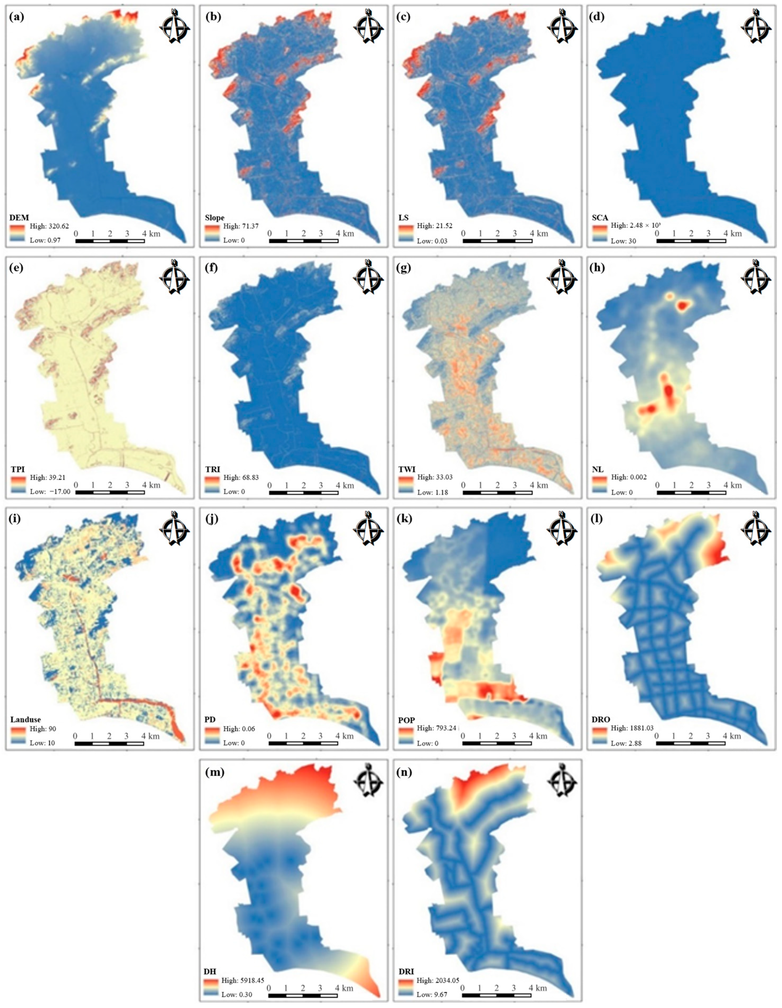
2.4.2. Explanatory Factors

To construct the mapping from predictor variables to inundation, 14 factors were selected based on literature review [16]. These explanatory variables reflect the local environmental features, namely the influence of local topography, hydrological features, local subsurface conditions, and anthropogenic factors. Spatial heterogeneity of rainfall is also an important factor in flood inundation, however, with reference to related studies [16], the spatial variability of rainfall is considered small on the small spatial scale of an urban center, and therefore rainfall indicators were not considered in the explanatory variables. The multi-source data were processed into a uniform raster with the same resolution. The data used were listed in Table 1. These factors were categorized as two types: (1) topographic and hydrologic factors; and (2) socioeconomic and anthropologic factors.
(1)
Topographic and hydrological factors
Topographic and hydrologic factors directly influence flow generation and flow routing, which are critical in hydrodynamic simulations of inundation. Based on the recent literature [16,37] and previous research [20,49], we adopted seven factors: Elevation, Slope, LS, SCA, TPI, TRI, and TWI.
Elevation (ranging from 0.97 m to 320.62 m, as shown in Figure 8a) is crucial for flooding [23]. Slope (ranging from 0° to 71.37°) is a terrain factor that reflects the change in elevation and affects flow direction and pluvial inundation. Higher values are distributed to the north of the Jin’an River, and lower values are found in the central urban district (Figure 8b). One of the most important driving factors of geomorphic processes and soil characteristics is the LS factor [52], which was calculated using SAGA GIS software (Figure 8c). SCA (Figure 8d) is a topographic index that represents the contributing catchment area for each grid cell. TPI (Figure 8e) indicates the difference between the elevation of each cell and the mean elevation of neighboring cells around the specific cell. TRI (Figure 8f) represents the roughness of the surface, which is useful in flood inundation modeling [16], and it provides an objective quantitative measure of topographic heterogeneity. TWI (ranging from 1.18 to 33.03, as shown in Figure 8g) combines the local upslope area contributing to the quantification of the topographic control on hydrological processes:
T W I = ln ( a tan b )
where a is the upstream contributing area; tan(b) represents the steepest downslope direction.
(2)
Socioeconomic and anthropologic factors
Socioeconomic and anthropologic factors describe the local factors related to human activities, which are not exactly the inherent property under natural conditions. They reflect that the urban environment is a dichotomy that requires consideration of both natural and human activities. Based on related literature [16,25], we adopted seven factors: NL, Landuse, PD, POP, DRO, DH, and DRI.
NL (Figure 8h) is the light produced by a city at night that can be detected using remote sensing technology, which reflects the level of human activity and social development. Sources of NL data comprise the Defense Meteorological Satellite Program Operational Line-Scan System (DMSP/OLS), the National Polar-orbiting Partnership Visible Infrared Imaging Radiometer Suite (NPP–VIIRS), and the LJ1-01 dataset. With a spatial resolution of 130 m, the LJ1-01 dataset is better than either the DMSP/OLS or the NPP-VIIRS dataset for application to urban analysis.
Land use (Figure 8i) serves as a forcing condition for hydrological modeling, and the various types of surfaces contribute differently to runoff generation. PD (Figure 8j) indicates the density of underground drainage channels, which directly affects pluvial flooding and inundation:
P D = 1 S i = 1 n L i
where S is the area of each grid; n is the number of conduits; Li is the conduit length.
PD reflects the population count, shown in Figure 8k. DRO (Figure 8l), DH (Figure 8m), and DRI (Figure 8n) represent the distances to roads, hospitals, and rivers, respectively, at each site, serving as indicators of human activity, risk avoidance during flood events, and proximity to water sources.

3. Results and Discussion

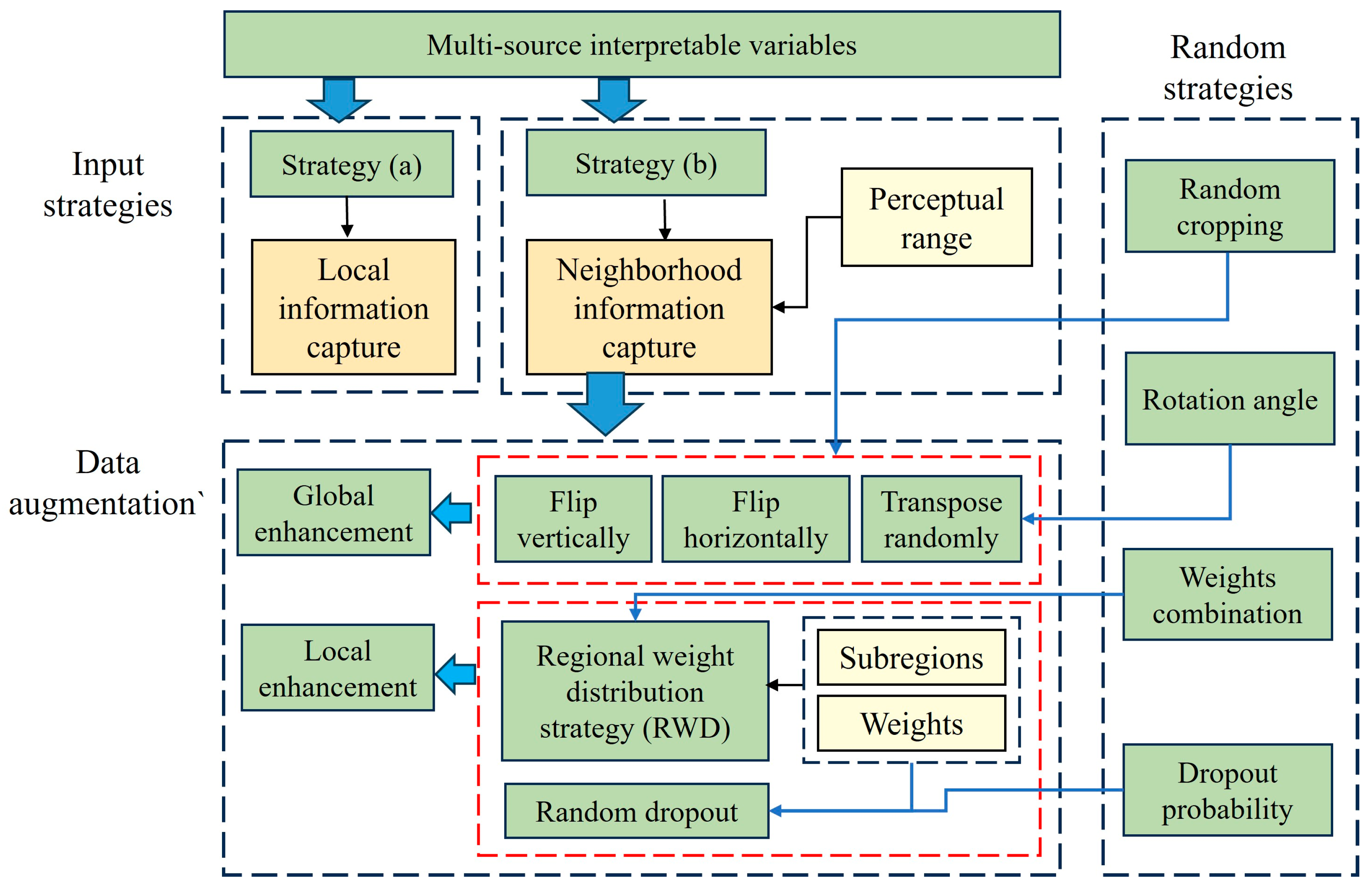
3.1. Performance Comparison Driven by Two Input Strategies

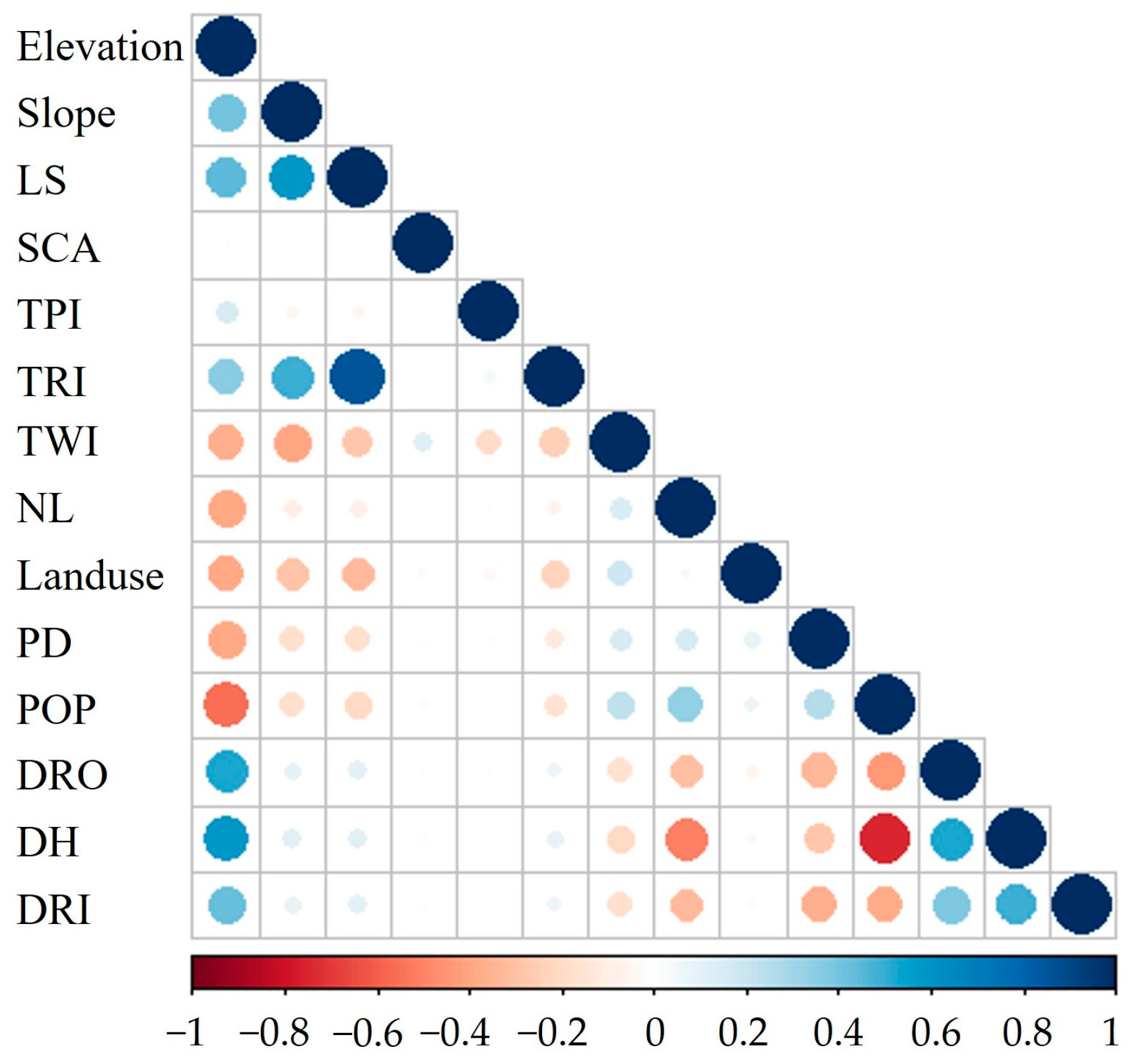
3.1.1. Correlation Analysis of Features

The predictor variables were selected based on anthropogenic, topographic, and socioeconomic factors. Given the large number of indicators, significant correlations between them could weaken the model’s generalization ability, even if it performed well on the training dataset. Thus, Pearson correlation analysis was performed for each explanatory variable. The results (Figure 9) revealed no significant correlation between any of the explanatory variables.

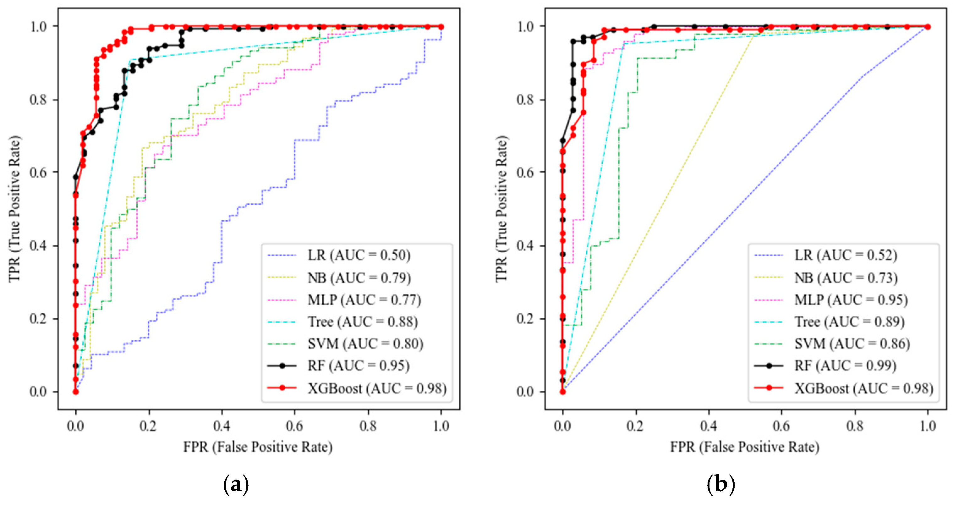
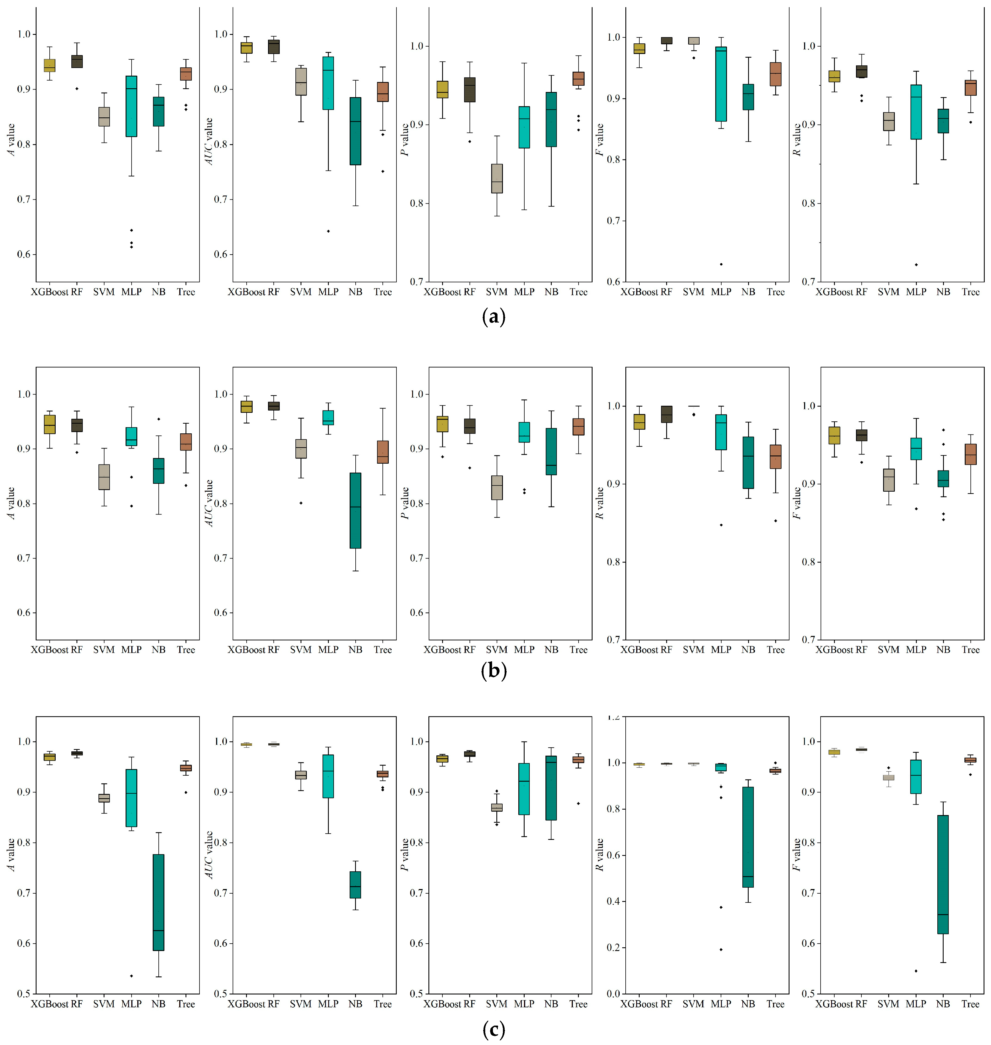
3.1.2. Performance Comparison by Two Strategies

The performance of the seven data-driven models under two input strategies is shown in Table 2, and four indicators for each model are discussed. Strategy (b) provides a wider perception range, with more information to learn. To compare to strategy (a), here a range of 15 m was used for neighborhood information extraction.
Apparently, in strategy (a), the integrated models (RF and XGBoost) outperform the relatively simple data-driven models (LR, NB, MLP, Tree, and SVM), and XGBoost performs best. The flood feature mapping involves 14 influential factors, with a relatively large parameter space. The more complex structure of the integrated model provides better performance. Strategy (b) takes the neighborhood information of the specified point into account based on strategy (a). The performance of each model was improved after extracting features with a window size of 30 m. The value of A for the LR model increased from 0.75 to 0.91. Similar to strategy (a), XGBoost performs best with the validation dataset based on all the indices.
The ROC curve and AUC values are presented in Figure 10. The AUC value refers to the area below the ROC curve. Generally, the effect of the AUC is improved by introducing the information of neighborhood features in the calculation, especially for MLP, SVM, and RF. After introducing the neighborhood information, RF and XGBoost have better performance, namely, 0.99 and 0.98, respectively.

3.2. Model Performance Based on Improved Feature Extracting Strategies

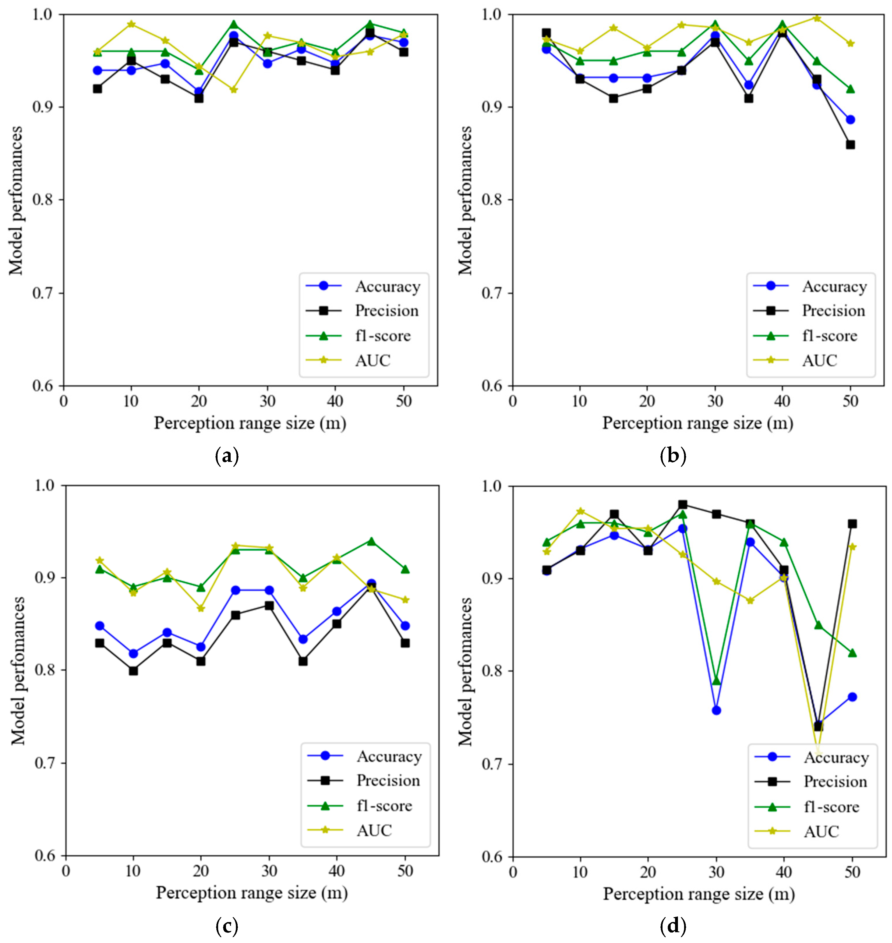
3.2.1. Perception Range Optimizing

The spatial information has autocorrelation, and the extraction of valid data is enhanced by introducing neighborhood information. Compared with watersheds, urban drainage areas have a smaller scale, and the neighborhood extent represents the extent to which information around a given point is used in the assessment. When too little neighborhood information is used, effective characterization of the neighborhood features cannot be represented. However, when too much neighborhood information is used, too much invalid information is introduced. Thus, it is necessary to analyze the size of neighborhood window and find the optimal perceptual range. Thus, 10 window sizes (5, 10, 15, 20, 25, 30, 35, 40, 45, and 50 m) were used, and the optimal size parameter was obtained based on the effects under given perceptual range.
The results presented in Section 3.1 indicate that XGBoost and RF are the two best-performing models, which are used to optimize the perceptual range. Moreover, we also conducted the same analysis on SVM and MLP with slightly weaker performance. The results show that the index R demonstrates relatively good performance in all cases. Therefore, four additional indices (P, A, F, and AUC) are employed to further evaluate the effects of perception ranges.
The four indices generated by the models are shown in Figure 11. The performance of each indicator varies as the perception range increases. Generally, the performance of MLP is relatively weak, especially when the perception range exceeds 20 m, where a significant decline in model performance is observed. The indices of XGBoost range from 0.9 to 1.0, those of RF range from 0.85 to 1.0, and those of SVM range from 0.8 to 0.92. Overall, when the perception range is less than 20 m, the model makes limited use of the information around the target point. When the perceptual range is larger than 35 m, the model performance fluctuates, and the comprehensive performance of the model starts to decrease. For XGBoost, which has a better ability to fit nonlinearities, the change characteristics are more obvious owing to its overall better performance. More neighborhood information is extracted by increasing the perceptual range, the amount of computation is substantially increased in the model learning process, and the information around the target point is fully used. However, incorporating too much information will not only introduce substantial invalid information or create a noisy computation but also could lead to overfitting and more computation.

3.2.2. Performance Improvements Through Data Augmentation

Data augmentation (AUG) is considered to further improve model performance, which is performed based on input strategy (b). For a specific perception range, when the images are flipped horizontally, flipped vertically, or transposed, the inundation features obtained from the mapping of explanatory variables remain unchanged. Therefore, we expanded the original dataset threefold using these three data augmentation methods to generate more mapping information between features and targets.
Similar to the previous sections, a better-performing model (XGBoost) and a weaker-performing model (SVM) based on strategy (b) are selected to present the performance. Four indicators (A, P, R, F) under various forcing conditions are illustrated in Figure 12. XGBoost can be seen to outperform SVM, and the overall performance of the model decreases when the window size changes from 25 to 50 m, consistent with the results of the previous analysis. For XGBoost, almost all performance indices are further optimized in various cases after employing data augmentation. However, for SVM, the effect played by increasing the computational effort of the training process is not obvious. It indicates that for more complex model structures and for models with better feature extraction, the increased computational effort allows the model to better extract features from multiple sources of data. Therefore, the increased number of training information from data augmentation allows the model to fit parameters with stronger generalization and robustness during training. However, for models with weaker performance, this approach has a smaller impact, the increased computations result in reduced computational efficiency in this case.

3.2.3. Performance Analysis Based on RWD and RD

Features closer to the target point contribute significantly more to their target flood-prone state. RWD is essentially a local enhancement strategy that amplifies the influence of nearby regions. Based on Equation (9), we assign three parameters ( λ 1 , λ 2 , λ 3 ) to reflect the weights of three subregions. As the sum of weights is 1, the three parameters are set to 0.5, 0.3, and 0.2. The three scenarios are as follows: (a) tests without additional improvements, (b) tests with RWD, and (c) tests coupled with RWD and RD. These tests were conducted with a random perception range from 5 m to 100 m, which introduced a certain degree of uncertainty in the results. Figure 13 shows the model performances in three scenarios. The prediction performance was slightly improved through RWD, specifically for MLP the performance improvement was significant. Scenario (c) presents significant improvements for the models, except for the NB model. The model performance is substantially improved across the various perception ranges. Additionally, under the combined effect of RWD and RD, the uncertainty of the model also shows a decreasing trend.

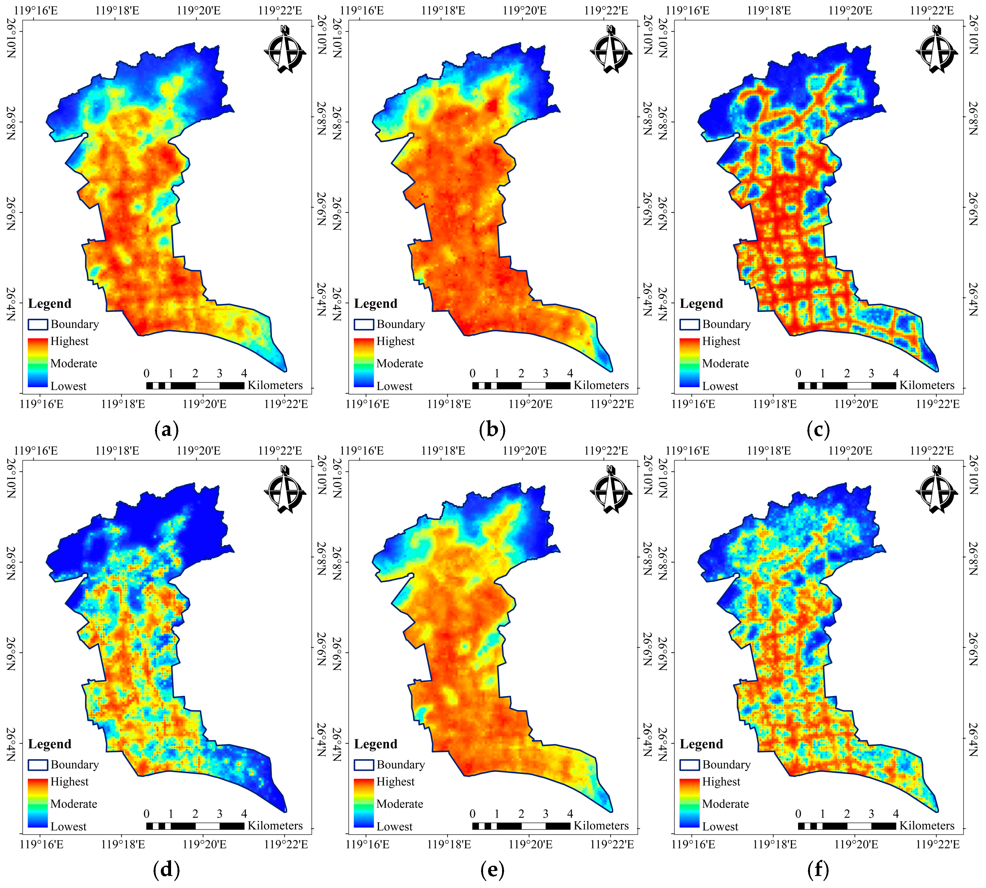
3.3. Flood Susceptibility Distribution

In this section, three models under strategy (a) and strategy (b) are presented. We select three data-driven models, which include models with better performance (XGBoost) and models with slightly weaker performance (MLP and SVM). The distribution of flood susceptibility in the study area is shown in Figure 14. The raster values in the figure represent the model’s output p , which ranges from 0 to 1 and reflects the degree of flood proneness. The larger the p value of a raster cell, the higher the risk of being flood-prone. Although the models under the two strategies consistently identify the distribution of flood-prone areas, there are some differences in their distribution results. Specifically, the flood-prone areas identified under strategy (b) have more distinct local texture characteristics than those identified under strategy (a). Moreover, there are more zones, with the highest risk and zones with the lowest risk under strategy (a). However, many areas in the actual urban area lie between absolute inundation and non-inundation. The flood-prone state changes dynamically with external conditions, and there is no absolute inundation and non-inundation point. When the driving strategy changes from (a) to (b), areas with the highest risk from XGBoost decreased from 21.82 to 15.01 km2, while the areas with the lowest risk decreased from 17.72 to 14.62 km2. By introducing local neighborhood information in the learning process, the local features are better extracted, and the results of strategy (b) show a clearer outline, while the sub-boundaries of each strategy category are fuzzier; that is, the performance concerning high-risk regions is improved significantly. By incorporating local neighborhood information, the features can be better extracted. The map of strategy (b) exhibits clearer contours and more detailed flood susceptibility distribution. The sub-boundaries of each strategy category are fuzzier, namely, the distribution of different risk levels is more detailed.
By extracting complex features such as hydrology, topography, and human activities, it is possible to capture the underlying patterns of the data. These implied features include not only the texture features of the high-risk areas mentioned above but also the local features of the low-risk areas. The northern part of the study area is connected to the mountainous areas, and the produced flow generally merges quickly into surrounding rivers, but ponding might still form in local depressions and residential areas. However, because of the low population density of the urban area upstream of Qinting Lake, relatively few inundation points are recorded. The insufficient learning ability of the model makes it easy for the model to assess the upstream mountainous areas as non-inundated areas directly (Figure 14f), while still providing prediction results after combining the explanatory variables.

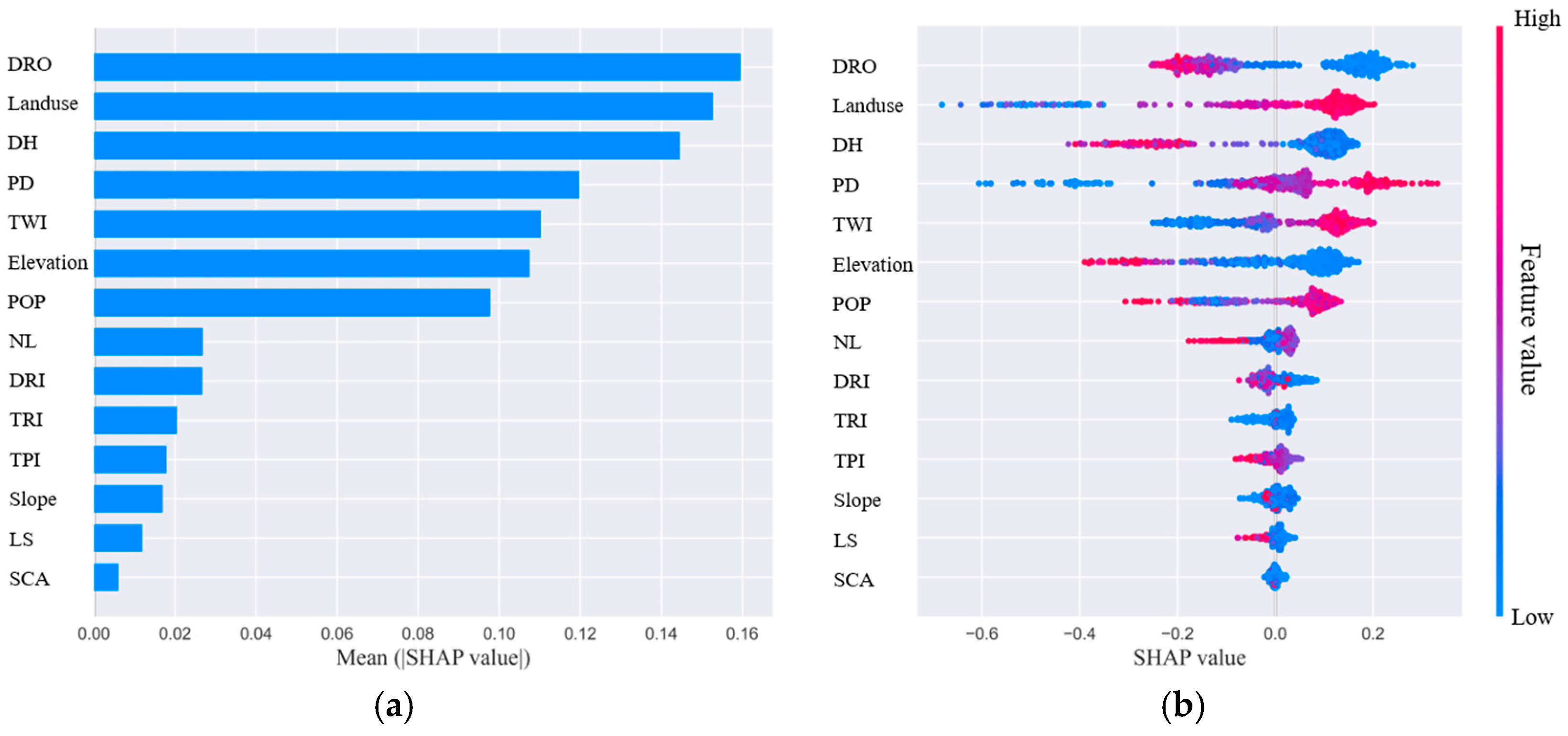
3.4. Driving Forces of Flood-Prone Areas

The effects of explanatory factors on the prediction results deserve further research. When the effect of an explanatory variable on the results is very weak, it can no longer be included in the model construction, which might provide better prediction performance. The SHAP values of each factor that contribute to the flood-prone areas on the global samples are shown in Figure 15. The specialized variables cause a loss in prediction value when the SHAP value is negative. DRO, Landuse, DH, PD, TWI, Elevation, and POP are the main factors driving a flood-prone site, while the remaining indices have significantly weaker effects. The mean SHAP values of the seven main influencing factors are in the range of 0.1–0.16. Specifically, the indices reflect topographical factors (TWI and Elevation), subsurface drainage characteristics (DRO, Landuse, and PD), and socioeconomic factors (DH and POP).
Moreover, DRO, Elevation, and DH (PD, TWI, and POP) have a negative (positive) relationship with flood-prone sites. Areas with drainage networks in urban regions are more likely to experience significant flow generation. This suggests a higher susceptibility to flooding caused by manhole overflow, particularly if the drainage capacity is insufficient. Moreover, the widespread presence of drainage networks generally reduces PD values, especially in mountainous areas with elevated terrain, which tend to experience less severe inundation during pluvial rainfall events, particularly in mountainous areas where river flooding is absent.
Analysis of the driving factors in three typical sites is presented in Figure 16. Site 1 is a flood-prone site located in the mountain areas, where the features push the prediction result from a base value of 1.067 to 0.27. Although other features present a negative effect on the flood-prone status, the location on the street and the local topographic features drive the flood-prone sites. Site 2 is a flood-prone site located in the central urban area. The result was pushed to 1.15, which indicates a prominent feature of inundation motivated by PD, DRO, Landuse, DRI, Slope, and DH. Among them, the impacts of PD, Landuse, and DRO are most significant for similar areas. Site 3 is a non-flood site, notably influenced by Elevation, Landuse, and PD.
The coupling effects of part of the main indexes are shown in Figure 17. When the Elevation is low, the change of DRO has a significant effect on the results. When the Elevation is relatively large, the contribution value becomes smaller as DRO increases. It means that for mountainous areas, distance from low-lying roads is not strongly correlated with susceptibility to inundation. However, in an urbanized area, the closer the distance to the road, the more likely the occurrence of flooding. This is also consistent with practical experience, where urban flooding generally occurs on roads that are generally more low-lying in comparison with residential areas and where water from numerous residential subareas is transported from the main roads under the roads, making urban streets more prone to flooding when overflows occur. The SHAP results show that DRO is crucial to the occurrence of floods, and its coupling with Elevation further indicates that the likelihood of these floods is mainly concentrated on low-lying roads in central urban areas.
The coupling effects between DRO and POP reflect that the distance to the road is very sensitive to urban flooding in areas of relatively high population density, while in mountainous areas with lower population density, the distance transforms to become not sensitive. The inhabitants are generally clustered in the urban plain areas with low elevation, which makes the red points in Figure 17f distributed in the range of horizontal coordinates 0–0.2. In contrast, in areas away from urban areas, elevation change is not the main factor driving inundation. Figure 17i represents the coupling of two terrain factors. High slope distributes in mountainous locations with high slopes, and increasing TWI can promote flooding in areas with lower slopes.

3.5. Discussion

3.5.1. Discussion on Multi-Resolution Modeling

Urban flood formation mechanisms are complex, especially in coastal cities, which may suffer from storm, flood, and tide levels simultaneously. Physical-based models are generally resolved in the whole flooding process. Thus, the hydrodynamic models are always used by coupling with hydrological models, which require extensive monitoring data [11]. The high-resolution hydrodynamic model derives the grid-averaged water volume by approximate Riemann solution to derive the grid-averaged numerical flux, which requires large numbers of computing resources [18]. En-XGBoost is proposed to generate the spatial distribution of flood-prone areas more efficiently on multiple resolutions.
En-XGBoost can easily implement multi-resolution simulations. We choose a typical flood-prone area (near the south bus station) and drive the model with higher resolutions (10 m, 30 m, 50 m). The result (Figure 18) shows that although the extent of the inundation zone is roughly similar, the local inundation features are more explicit after increasing the grid density, which helps to identify the local inundation zone. When the computational grid resolution increases, there are correspondingly more points to be predicted. For the data-driven model, the training process consumes more computational resources due to the need for parameter calibration, whereas for the prediction of unknown points there is no need for complex parameter correction. In contrast, the high-resolution hydrodynamic model needs to calculate the numerical fluxes in each time step, and the more effective grids lead to the more complex calculation.

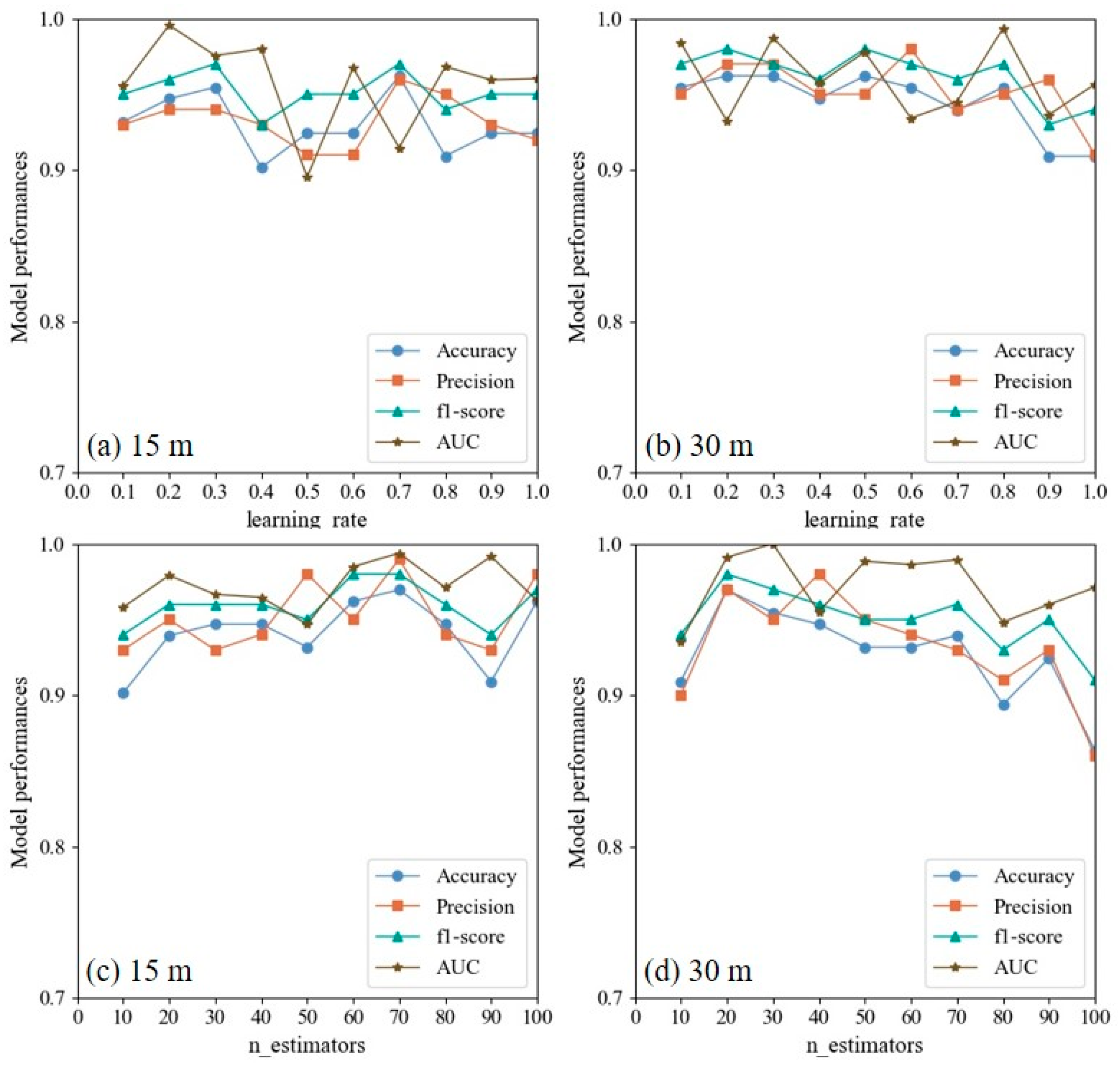
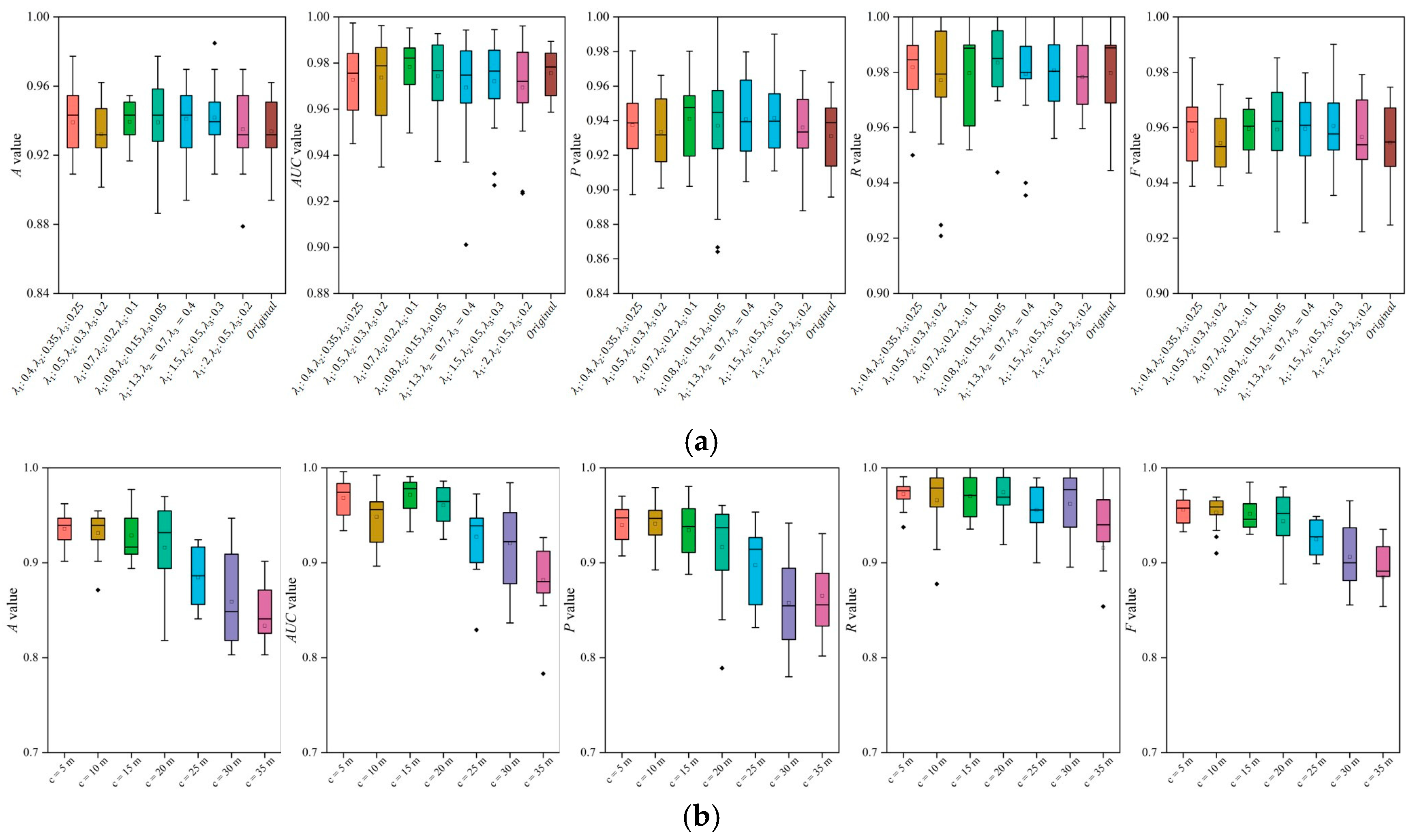
3.5.2. Discussion of Hyperparameters of En-XGBoost

The impact of the main hyperparameters of En-XGBoost was analyzed and is shown in Figure 19. The discussion primarily focuses on two parameters: learning rate (LR) and n_estimators (NE). Increasing LR makes the model training faster, however, it may fall into local optimal points. To make the model neither overfitting nor underfitted, a suitable NE is needed. LR was set to 0.3 and NE was set to 70. It appears that the model shows relatively low sensitivity to parameters that vary around the selected values.
The parameters of En-XGBoost also contain the weights for subregions according to RWD. Figure 20a gives the model performance to various series of weights combinations. Due to the incorporation of neighborhood information, XGBoost effectively captures the local flood features. Although the models perform relatively well under all schemes, the right combination of parameters (e.g., λ 1 : 0.8 , λ 2 : 0.15 , λ 3 : 0.05 ;   λ 1 : 1.3 , λ 2 : 0.7 , λ 3 : 0.4 ) is effective in enhancing the evaluation metrics.
Furthermore, Figure 20b provides the model performance forcing by RD. Specifically, the performance decreases rapidly after c is greater than 25. With this strategy, information at a distance is randomly discarded in part. The randomly incorporated neighborhood information plays the role of a regular term, which can correct the locally fused information and avoid the overfitting phenomenon. Nonetheless, this strategy is not continuously effective; when too much information is randomly incorporated, this instead destroys the original spatial structure features and topological connections, leading to the degradation of model performance. Therefore, different stochastic strategies, neighborhood distances, and parameter combinations should be carefully integrated based on the specific situation.

3.5.3. Future Work

Although the random strategies extract neighborhood information from around a specific site, there is still a certain loss of the original spatial topological relationship in the calculation, which could be considered for improvement by adding convolutional structures. Features extracted through convolutional operations retain spatial topological relationships and perform information fusion via filters. Despite the increased computational cost, this approach offers a promising option for performance improvement. However, the local enhancement method used in this paper provides an alternative way for feature extraction and fusion. Moreover, the interpretable factors were derived from literature reviews and correlation analysis, with no significant correlations identified among the indicators. Data-driven models often require extensive computations, many of which may be invalid when explanatory variables have minimal impact on the results. To improve computational efficiency, future work could focus on retaining the most influential factors while disregarding those of lesser importance, thereby enhancing the effectiveness of nonlinear mappings.

4. Conclusions

The main conclusions can be summarized as follows.
(1)
Incorporating the characteristics of local information around a specified point has a positive impact, improving the generalization ability of the model. However, there is a limit regarding the introduction of neighborhood information; information that is far away from inundation sites is not sufficiently relevant to the inundation characteristics of the specified point.
(2)
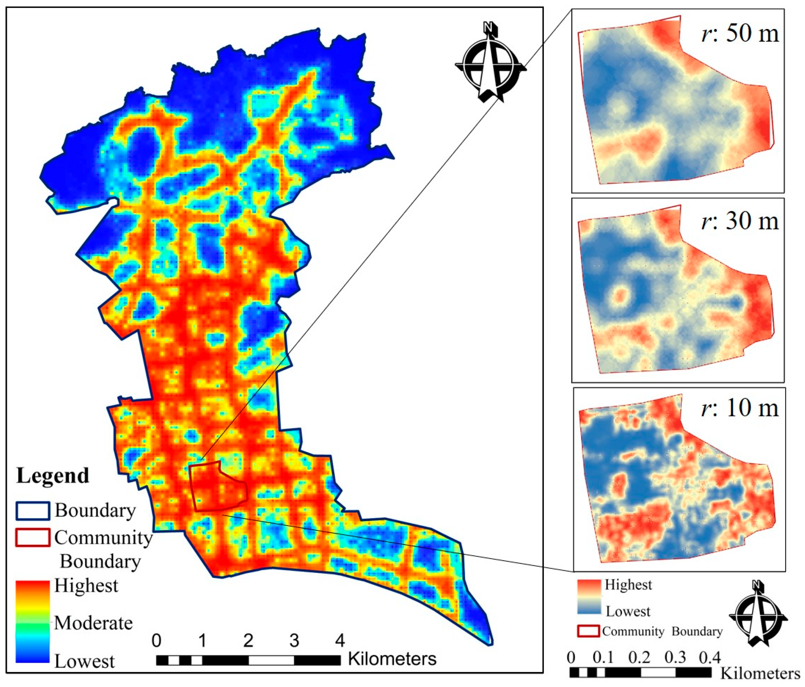
Two strategies considered both successfully provided the flooding distribution; however, strategy (b) extracts texture features of the flood distribution in greater detail, producing clearer boundaries between areas of different levels of flood susceptibility. In changing the forcing from strategy (a) to (b), the areas recognized as highest risk decreased from 21.82 to 15.01 km2, while the areas labeled as lowest risk decreased from 17.72 to 14.62 km2.
(3)
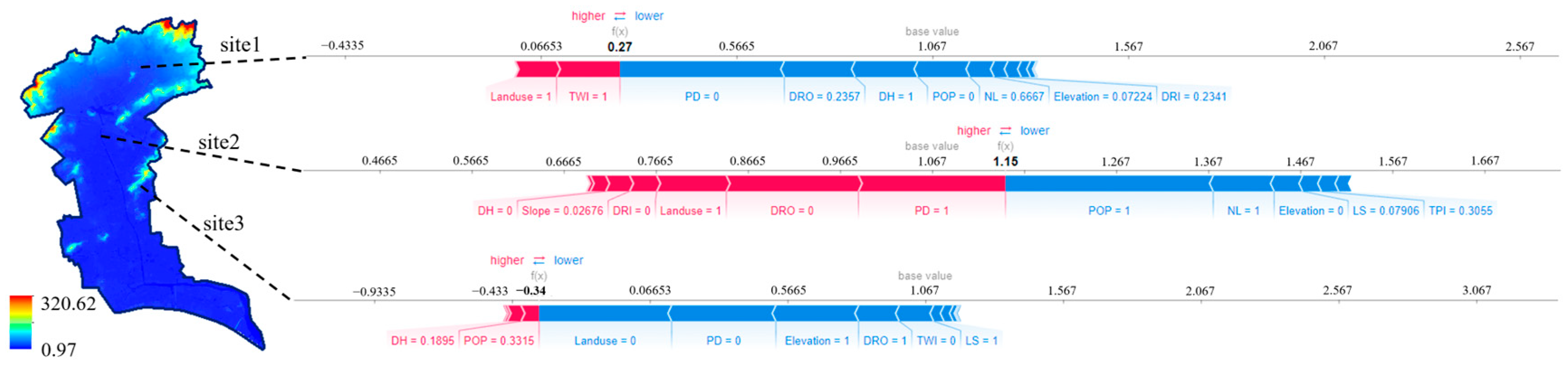
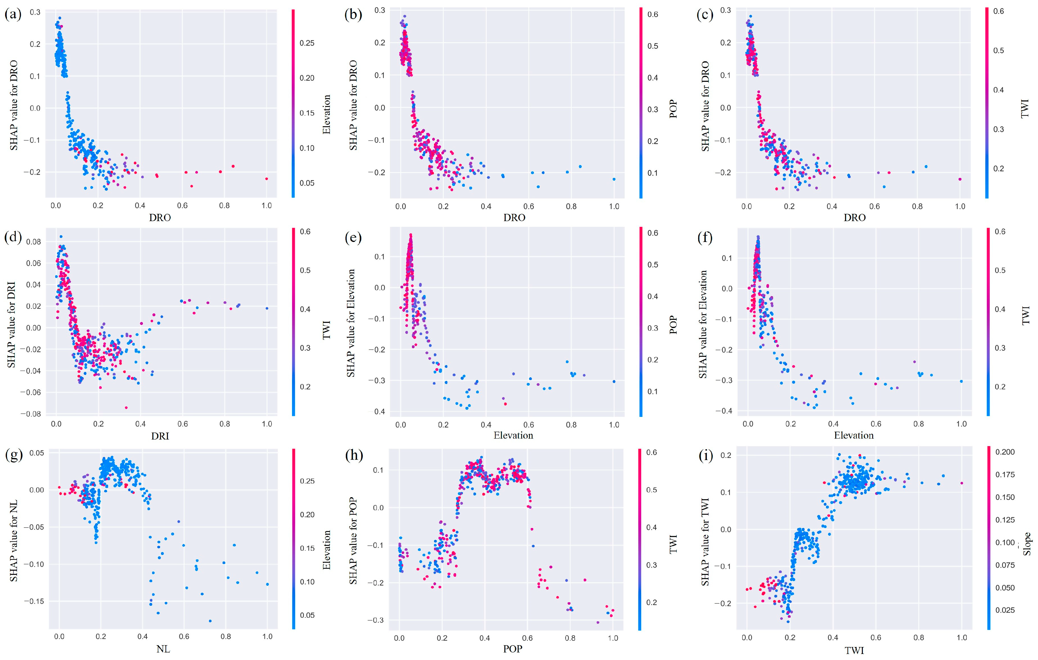
The indices of DRO, Land use, DH, PD, TWI, Elevation, and POP were recognized as the main factors that affect the prediction. For specific sites in different locations, there are differences in their main driving factors. The analysis of their flooding causes in combination with their locations can effectively help improve understanding of flood risk.
(4)
Data augmentation proves to be beneficial for stronger models, while its impact is less pronounced for weaker models. The random strategies enhance the framework’s generalization by increasing the randomness in local feature extraction. In practical applications, the decision to incorporate sufficient random strategies and data augmentation should depend on the complexity of the training data and the model structure.

Author Contributions

Conceptualization, C.Y., Z.X. and W.L.; Methodology, C.Y.; Software, X.S.; Validation, Z.X. and X.S.; Formal analysis, W.L. and X.L.; Investigation, Z.X., W.L., X.L. and X.S.; Resources, W.L. and X.L.; Data curation, W.L.; Writing—original draft, C.Y.; Writing—review & editing, C.Y., Z.X. and X.S.; Visualization, C.Y.; Supervision, Z.X. and X.L.; Project administration, C.Y.; Funding acquisition, C.Y. All authors have read and agreed to the published version of the manuscript.

Funding

This study was supported by the National Natural Science Foundation of China (52409005), the China Postdoctoral Science Foundation (2024M750224), and the National Natural Science Foundation of China (52239003).

Institutional Review Board Statement

Not applicable.

Informed Consent Statement

Not applicable.

Data Availability Statement

The original contributions presented in the study are included in the article, further inquiries can be directed to the corresponding author.

Conflicts of Interest

The authors declare that they have no known competing financial interest or personal relationships that could have appeared to influence the work reported in this paper.

References

  1. Yin, J.; Ye, M.; Yin, Z.; Xu, S. A review of advances in urban flood risk analysis over China. Stoch. Environ. Res. Risk Assess. 2014, 29, 1063–1070. [Google Scholar] [CrossRef]
  2. Koks, E. Moving flood risk modelling forwards. Nat. Clim. Change 2018, 8, 561–562. [Google Scholar] [CrossRef]
  3. Fang, J.; Wahl, T.; Fang, J.; Sun, X.; Kong, F.; Liu, M. Compound flood potential from storm surge and heavy precipitation in coastal China: Dependence, drivers, and impacts. Hydrol. Earth Syst. Sci. 2021, 25, 4403–4416. [Google Scholar] [CrossRef]
  4. Tehrany, M.S.; Lee, M.-J.; Pradhan, B.; Jebur, M.N.; Lee, S. Flood susceptibility mapping using integrated bivariate and multivariate statistical models. Environ. Earth Sci. 2014, 72, 4001–4015. [Google Scholar] [CrossRef]
  5. Yin, J.; Yu, D.; Wilby, R. Modelling the impact of land subsidence on urban pluvial flooding: A case study of downtown Shanghai, China. Sci. Total Environ. 2016, 544, 744–753. [Google Scholar] [CrossRef]
  6. Yin, J.; Yu, D.; Yin, Z.; Liu, M.; He, Q. Evaluating the impact and risk of pluvial flash flood on intra-urban road network: A case study in the city center of Shanghai, China. J. Hydrol. 2016, 537, 138–145. [Google Scholar] [CrossRef]
  7. Anni, A.H.; Cohen, S.; Praskievicz, S. Sensitivity of urban flood simulations to stormwater infrastructure and soil infiltration. J. Hydrol. 2020, 588, 125028. [Google Scholar] [CrossRef]
  8. Ferreira, C.S.; Walsh, R.P.; Steenhuis, T.S.; Ferreira, A.J. Effect of peri-urban development and lithology on streamflow in a mediterranean catchment. Land Degrad. Dev. 2017, 29, 1141–1153. [Google Scholar] [CrossRef]
  9. Hou, J.; Zhou, N.; Chen, G.; Huang, M.; Bai, G. Rapid forecasting of urban flood inundation using multiple machine learning models. Nat. Hazards 2021, 108, 2335–2356. [Google Scholar] [CrossRef]
  10. Xie, K.; Ozbay, K.; Zhu, Y.; Yang, H. Evacuation zone modeling under climate change: A data-driven method. J. Infrastruct. Syst. 2017, 23, 04017013. [Google Scholar] [CrossRef]
  11. Xu, Z.; Ye, C. Simulation of urban flooding/waterlogging processes: Principle, models and prospects. J. Hydraul. Eng. 2021, 52, 381–392. [Google Scholar]
  12. Rubinato, M.; Shucksmith, J.; Saul, A.J.; Shepherd, W. Comparison between InfoWorks hydraulic results and a physical model of an urban drainage system. Water Sci. Technol. 2013, 68, 372–379. [Google Scholar]
  13. Fan, Y.; Ao, T.; Yu, H.; Huang, G.; Li, X. A Coupled 1D-2D Hydrodynamic Model for Urban Flood Inundation. Adv. Meteorol. 2017, 2017, 2819308. [Google Scholar] [CrossRef]
  14. Mei, C.; Liu, J.; Wang, H.; Li, Z.; Xia, L.; Wang, Y. Introduction of basic principle and application prospect for SWMM. Water Resour. Hydropower Eng. 2017, 48, 33–42. [Google Scholar]
  15. Tu, M.-C.; Smith, P. Modeling Pollutant Buildup and Washoff Parameters for SWMM Based on Land Use in a Semiarid Urban Watershed. Water Air Soil Pollut. 2018, 229, 121. [Google Scholar] [CrossRef]
  16. Lei, X.; Chen, W.; Panahi, M.; Falah, F.; Rahmati, O.; Uuemaa, E.; Kalantari, Z.; Ferreira, C.S.S.; Rezaie, F.; Tiefenbacher, J.P.; et al. Urban flood modeling using deep-learning approaches in Seoul, South Korea. J. Hydrol. 2021, 601, 126684. [Google Scholar] [CrossRef]
  17. Ye, C.; Xu, Z. Simulation of fluvial/pluvial flooding processes in a typical urban area considering role of low impact development (LID) measures and joint operation for hydraulic structures: Case study in Fuzhou City. J. Hydraul. Eng. 2022, 53, 833–844. [Google Scholar]
  18. Liang, Q.; Xia, X.; Hou, J. Catchment-scale high-resolution flash flood simulation using the GPU-based technology. Procedia Eng. 2016, 154, 975–981. [Google Scholar]
  19. Xing, Y.; Liang, Q.; Wang, G.; Ming, X.; Xia, X. City-scale hydrodynamic modelling of urban flash floods: The issues of scale and resolution. Nat. Hazards 2018, 96, 473–496. [Google Scholar]
  20. Ye, C.; Xu, Z.; Lei, X.; Liao, W.; Ding, X.; Liang, Y. Assessment of urban flood risk based on data-driven models: A case study in Fuzhou City, China. Int. J. Disaster Risk Reduct. 2022, 82, 103318. [Google Scholar]
  21. Lee, S.; Lee, S.; Lee, M.J.; Jung, H.S. Spatial assessment of urban flood susceptibility using data mining and geographic information System (GIS) tools. Sustainability 2018, 10, 648. [Google Scholar] [CrossRef]
  22. Wang, Y.; Hong, H.; Chen, W.; Li, S.; Panahi, M.; Khosravi, K.; Shirzadi, A.; Shahabi, H.; Panahi, S.; Costache, R. Flood susceptibility mapping in Dingnan County (China) using adaptive neuro-fuzzy inference system with biogeography based optimization and imperialistic competitive algorithm. J. Environ. Manag. 2019, 247, 712–729. [Google Scholar] [CrossRef] [PubMed]
  23. Zhang, S.; Pan, B. An urban storm-inundation simulation method based on GIS. J. Hydrol. 2014, 517, 260–268. [Google Scholar] [CrossRef]
  24. Chen, W.; Wang, W.; Huang, G.; Wang, Z.; Lai, C.; Yang, Z. The capacity of grey infrastructure in urban flood management: A comprehensive analysis of grey infrastructure and the green-grey approach. Int. J. Disaster Risk Reduct. 2021, 54, 102045. [Google Scholar] [CrossRef]
  25. Zhao, G.; Pang, B.; Xu, Z.; Peng, D.; Xu, L. Assessment of urban flood susceptibility using semi-supervised machine learning model. Sci. Total. Environ. 2019, 659, 940–949. [Google Scholar] [CrossRef]
  26. Tehrany, M.S.; Pradhan, B.; Mansor, S.; Ahmad, N. Flood susceptibility assessment using GIS-based support vector machine model with different kernel types. Catena 2015, 125, 91–101. [Google Scholar] [CrossRef]
  27. Wang, Z.; Lai, C.; Chen, X.; Yang, B.; Zhao, S.; Bai, X. Flood hazard risk assessment model based on random forest. J. Hydrol. 2015, 527, 1130–1141. [Google Scholar] [CrossRef]
  28. Jin, H.; Zhao, Y.; Lu, P.; Zhang, S.; Chen, Y.; Zheng, S.; Zhu, Z. Using Machine Learning to Identify and Optimize Sensitive Parameters in Urban Flood Model Considering Subsurface Characteristics. Int. J. Disaster Risk Sci. 2024, 15, 116–133. [Google Scholar] [CrossRef]
  29. Zhao, G.; Pang, B.; Xu, Z.; Peng, D.; Zuo, D. Urban flood susceptibility assessment based on convolutional neural networks. J. Hydrol. 2020, 590, 125235. [Google Scholar] [CrossRef]
  30. Zhao, G.; Pang, B.; Xu, Z.; Yue, J.; Tu, T. Mapping flood susceptibility in mountainous areas on a national scale in China. Sci. Total. Environ. 2018, 615, 1133–1142. [Google Scholar] [CrossRef]
  31. Xu, H.; Ma, C.; Lian, J.; Xu, K.; Chaima, E. Urban flooding risk assessment based on an integrated k-means cluster algorithm and improved entropy weight method in the region of Haikou, China. J. Hydrol. 2018, 563, 975–986. [Google Scholar]
  32. Huang, H.; Chen, X.; Wang, X.; Wang, X.; Liu, L. A Depression-based index to represent topographic control in urban pluvial flooding. Water 2019, 11, 2115. [Google Scholar] [CrossRef]
  33. Mojaddadi, H.; Pradhan, B.; Nampak, H.; Ahmad, N.; Ghazali, A.H.B. Ensemble machine-learning-based geospatial approach for flood risk assessment using multi-sensor remote-sensing data and GIS. Geomat. Nat. Hazards Risk 2017, 8, 1080–1102. [Google Scholar]
  34. Nachappa, T.G.; Piralilou, S.T.; Gholamnia, K.; Ghorbanzadeh, O.; Rahmati, O.; Blaschke, T. Flood susceptibility mapping with machine learning, multi-criteria decision analysis and ensemble using Dempster Shafer Theory. J. Hydrol. 2020, 590, 125275. [Google Scholar]
  35. Hosseiny, H.; Nazari, F.; Smith, V.; Nataraj, C. A Framework for modeling flood depth using a hybrid of hydraulics and machine learning. Sci. Rep. 2020, 10, 8222. [Google Scholar]
  36. Chen, T.; Guestrin, C. Xgboost: A scalable tree boosting system. In Proceedings of the 22nd ACM SIGKDD International Conference on Knowledge Discovery and Data Mining, San Francisco, CA, USA, 13–17 August 2016; pp. 785–794. [Google Scholar]
  37. Ma, M.; Zhao, G.; He, B.; Li, Q.; Dong, H.; Wang, S.; Wang, Z. XGBoost-based method for flash flood risk assessment. J. Hydrol. 2021, 598, 126382. [Google Scholar]
  38. Meng, Y.; Yang, N.; Qian, Z.; Zhang, G. What makes an online review more helpful: An interpretation framework using XGBoost and SHAP values. J. Theor. Appl. Electron. Commer. Res. 2020, 16, 466–490. [Google Scholar] [CrossRef]
  39. Feng, D.-C.; Wang, W.-J.; Mangalathu, S.; Taciroglu, E. Interpretable XGBoost-SHAP machine-learning model for shear strength prediction of Squat RC walls. J. Struct. Eng. 2021, 147, 04021173. [Google Scholar]
  40. Guo, M.; Yuan, Z.; Janson, B.; Peng, Y.; Yang, Y.; Wang, W. Older Pedestrian Traffic Crashes Severity Analysis Based on an Emerging Machine Learning XGBoost. Sustainability 2021, 13, 926. [Google Scholar] [CrossRef]
  41. Wang, S.; Peng, H.; Hu, Q.; Jiang, M. Analysis of runoff generation driving factors based on hydrological model and interpretable machine learning method. J. Hydrol. Reg. Stud. 2022, 42, 101139. [Google Scholar]
  42. Xu, Z.; Ye, C. From “looking at sea in city” to “looking at river in city”: Simulation and risk analysis of flood and waterlogging process in Fuzhou City under extreme rainstorm scenarios. China Flood Drought Manag. 2021, 9, 12–20. [Google Scholar]
  43. Wu, C.L.; Chau, K.W.; Li, Y.S. Predicting monthly streamflow using data-driven models coupled with data-preprocessing tech-niques. Water Resour. Res. 2009, 45. [Google Scholar] [CrossRef]
  44. Tang, X.; Hong, H.; Shu, Y.; Tang, H.; Li, J.; Liu, W. Urban waterlogging susceptibility assessment based on a PSO-SVM method using a novel repeatedly random sampling idea to select negative samples. J. Hydrol. 2019, 576, 583–595. [Google Scholar]
  45. Rizeei, H.M.; Pradhan, B.; Saharkhiz, M.A.; Lee, S. Groundwater aquifer potential modeling using an ensemble multi-adoptive boosting logistic regression technique. J. Hydrol. 2019, 579, 124172. [Google Scholar]
  46. Desai, S.; Ouarda, T.B. Regional hydrological frequency analysis at ungauged sites with random forest regression. J. Hydrol. 2021, 594, 125861. [Google Scholar]
  47. Pham, B.T.; Jaafari, A.; Van Phong, T.; Mafi-Gholami, D.; Amiri, M.; Van Tao, N.; Duong, V.-H.; Prakash, I. Naïve Bayes ensemble models for groundwater potential mapping. Ecol. Inform. 2021, 64, 101389. [Google Scholar] [CrossRef]
  48. Schoppa, L.; Disse, M.; Bachmair, S. Evaluating the performance of random forest for large-scale flood discharge simulation. J. Hydrol. 2020, 590, 125531. [Google Scholar] [CrossRef]
  49. Ye, C.; Xu, Z.; Lei, X.; Zhang, R.; Chu, Q.; Li, P.; Ban, C. Assessment of the impact of urban water system scheduling on urban flooding by using coupled hydrological and hydrodynamic model in Fuzhou City, China. J. Environ. Manag. 2022, 321, 115935. [Google Scholar]
  50. Liang, Y.; Liao, W.; Zhang, Z.; Li, H.; Wang, H. Using a multiphysics coupling-oriented flood modelling approach to assess urban flooding under various regulation scenarios combined with rainstorms and tidal effects. J. Hydrol. 2024, 645, 132189. [Google Scholar]
  51. Ye, C.; Xu, Z.; Lei, X.; Liao, W.; Li, P. Coupling simulation of hydrological and hydrodynamics processes for urban river networks based on InfoWorks: Case of the urban area and the northeast mountainous area in Fuzhou City. J. Beijing Norm. Univ. 2019, 5, 609–616. [Google Scholar]
  52. Khanifar, J.; Khademalrasoul, A. Multiscale comparison of LS factor calculation methods based on different flow direction algorithms in Susa Ancient landscape. Acta Geophys. 2020, 68, 783–793. [Google Scholar] [CrossRef]
Figure 1. Architecture of the study.
Sustainability 17 03065 g001
Figure 2. Flowchart of the core model.
Sustainability 17 03065 g002
Figure 3. Diagram of the components in the preprocessing module.
Sustainability 17 03065 g003
Figure 4. Random strategies and local enhancement.
Sustainability 17 03065 g004
Figure 5. Urban pluvial flooding process.
Sustainability 17 03065 g005
Figure 6. Map of the study area showing locations of flood site samples.
Sustainability 17 03065 g006
Figure 7. Calibration and validation periods of the PBM.
Sustainability 17 03065 g007
Figure 8. The interpretable features of the study area: (a) Elevation, (b) Slope, (c) LS, (d) SCA, (e) TPI, (f) TRI, (g) TWI, (h) NL, (i) Landuse, (j) PD, (k) POP, (l) DRO, (m) DH, and (n) DRI.
Sustainability 17 03065 g008
Figure 9. Correlation coefficient heat map.
Sustainability 17 03065 g009
Figure 10. Model performance compared with baseline models forced by two input strategies: (a) strategy (a), (b) strategy (b).
Sustainability 17 03065 g010
Figure 11. Model performance forcing by different perception range sizes: (a) XGBoost, (b) RF, (c) SVM, and (d) MLP.
Sustainability 17 03065 g011
Figure 12. Heatmap of the performances of a series of models under several forcing conditions.
Sustainability 17 03065 g012
Figure 13. Model performances under local enhancement improvements: (a) Scenario (a), (b) Scenario (b), and (c) Scenario (c).
Sustainability 17 03065 g013
Figure 14. Flood susceptibility distribution forced by: (a) MLP + strategy (a), (b) SVM + strategy (a), (c) XGBoost + strategy (a), (d) MLP + strategy (b), (e) SVM + strategy (b), and (f) XGBoost + strategy (b).
Sustainability 17 03065 g014
Figure 15. Mean importance of interpretable factors: (a) Feature importance, and (b) SHAP value for each feature.
Sustainability 17 03065 g015
Figure 16. Driving factor analysis of three typical sites.
Sustainability 17 03065 g016
Figure 17. Coupling effects of the indices: (a) DRO and Elevation, (b) DRO and POP, (c) DRO and TWI, (d) DRI and TWI, (e) Elevation and POP, (f) Elevation and TWI, (g) NL and Elevation, (h) POP and TWI, and (i) TWI and Slope.
Sustainability 17 03065 g017
Figure 18. Simulations on multiple resolutions.
Sustainability 17 03065 g018
Figure 19. Performances response to hyperparameters: (a) learning rate, 15 m, (b) learning rate, 30 m, (c) n_estimators, 15 m, and (d) n_estimators, 30 m.
Sustainability 17 03065 g019
Figure 20. Performances response: (a) various weights combinations, and (b) random strategy.
Sustainability 17 03065 g020
Table 1. Data description.
NumberDataSpatial ResolutionSourceDescription
1Elevation2 mFuzhou Survey BureauDigital elevation model (DEM)
2Slope2 mProcessed from ArcGIS 10.5Slope of each grid
3LS2 mProcessed from SAGA GIS 9.3.1Landscape factor
4SCA2 mProcessed from ArcGIS 10.5Specific catchment area
5TPI2 mProcessed from ArcGIS 10.5Topographic position index
6TRI2 mProcessed from SAGA GIS 9.3.1Terrain ruggedness index
7TWI2 mProcessed from ArcGIS 10.5Topographic wetness index
8NL130 mLJ1-01 datasetNighttime light
9Landuse10 mFuzhou Survey BureauLand use
10PD5 mProcessed from ArcGIS 10.5Pipeline density
11POP100 mObtained from worldpop.orgPopulation count
12DRO5 mProcessed from ArcGIS 10.5Distance to the road
13DH5 mProcessed from ArcGIS 10.5Distance to the hospital
14DRI5 mProcessed from ArcGIS 10.5Distance to the river
Table 2. Model performance with the validation dataset.
ModelStrategy (a)Strategy (b)
APRFAPRF
LR0.750.750.950.840.910.930.960.95
NB0.720.830.810.820.820.840.940.88
MLP0.810.860.890.870.900.90.970.93
Tree0.880.930.920.920.900.930.950.94
SVM0.790.781.00.880.860.841.00.91
RF0.880.880.970.920.930.940.970.96
XGBoost0.910.930.940.930.940.931.00.97
Disclaimer/Publisher’s Note: The statements, opinions and data contained in all publications are solely those of the individual author(s) and contributor(s) and not of MDPI and/or the editor(s). MDPI and/or the editor(s) disclaim responsibility for any injury to people or property resulting from any ideas, methods, instructions or products referred to in the content.

