Article

Flue Gas Oxygen Content Model Based on Bayesian Optimization Main–Compensation Ensemble Algorithm in Municipal Solid Waste Incineration Process

1
School of Information Science and Technology, Beijing University of Technology, Beijing 100124, China
2
Beijing Laboratory of Smart Environmental Protection, Beijing 100124, China
*
Author to whom correspondence should be addressed.
Sustainability 2025, 17(7), 3048; https://doi.org/10.3390/su17073048
Submission received: 8 January 2025 / Revised: 23 March 2025 / Accepted: 26 March 2025 / Published: 29 March 2025
(This article belongs to the Section Waste and Recycling)

Abstract

:
The municipal solid waste incineration (MSWI) process plays a crucial role in managing the risks associated with waste accumulation and promoting the sustainable development of urban environments. However, unstable operation of the MSWI process can lead to excessive pollutant emissions, deteriorating air quality, and adverse impacts on public health. Flue gas oxygen content is a key controlled variable in the MSWI process, and its stable control is closely linked to both incineration efficiency and pollutant emissions. Developing a high-precision, interpretable model for flue gas oxygen content is essential for achieving optimal control. However, existing methods face challenges such as poor interpretability, low accuracy, and the complexity of manual hyperparameter tuning. To address these issues, this article proposes a flue gas oxygen content model based on a Bayesian optimization (BO) main–compensation ensemble modeling algorithm. The model first utilizes an ensemble TS fuzzy regression tree (EnTSFRT) to construct the main model. Then, a long short-term memory network (LSTM) is employed to build the compensation model, using the error of the EnTSFRT model as the target value. The final output is obtained through a weighted combination of the main and compensation models. Finally, the hyperparameters of the main–compensation ensemble model are optimized using the BO algorithm to achieve a high generalization performance. Experimental results based on real MSWI process data demonstrate that the proposed method performs well, achieving a 48.2% reduction in RMSE and a 53.1% reduction in MAE, while R2 increases by 140.8%, compared to the BO-EnTSFRT method that uses only the main model.

1. Introduction

One of the key challenges for the sustainable development of both the economy and the environment is effective pollutant control and CO2 emission reduction [1,2]. Municipal solid waste (MSW) generation continues to grow annually with the advancement of urbanization [3]. In developing countries, particularly in China, this growth has been especially rapid [4], leading to the phenomenon of “garbage siege” in many cities [5]. In alignment with the goals of sustainable urban development and the pursuit of “carbon peak and carbon neutrality”, effective MSW management has become an urgent priority in many countries [6].
Currently, MSW incineration (MSWI) is widely used as one of the primary waste-to-energy (WTE) technologies [7]. It offers several advantages, including waste reduction and the elimination of harmful substances [8,9], thereby supporting the sustainable development of urban environments. Additionally, using MSW to generate electricity helps reduce reliance on thermal power generation, contributing to carbon emission reduction [4]. However, the unstable operation of this process can lead to excessive pollutant emissions [10]. Research on waste incineration and optimization mainly focuses on using high-temperature incineration technology to treat MSW, in order to reduce waste volume, lower harmful substance emissions, and recover energy. The incineration process is not only an effective method for waste management but also contributes to sustainable energy production through energy recovery. With technological advancements, optimizing the incineration process through advanced control systems and artificial intelligence (AI)-driven monitoring techniques has become crucial, aiming to maximize environmental and economic benefits in a sustainable manner [11]. As a result, research into leveraging AI for pollution control and sustainable development has become a key area of focus [12].
The components of MSW are complex and can be categorized into four main types: recyclable materials (such as waste paper, glass, metal, etc.), kitchen waste (including leftovers, vegetable stems, tea stalks, etc.), harmful waste (such as battery, hair dye, waste the paint can, etc.), and other waste (such as shell, dust, cigarette, etc.) [13]. The complex composition of MSW can impact the stability of the MSWI process, making it more difficult to control. In the MSWI process, flue gas oxygen content is a key controlled variable (CV) that directly influences both incineration efficiency and pollutant emissions [14]. Maintaining the flue gas oxygen content within the specified range is essential for ensuring both high combustion efficiency and environmental protection. If the oxygen content is too low, the combustion efficiency decreases significantly, leading to the generation of harmful and toxic gases, such as dioxins (DXNs) and sulfur dioxide (SO2) [15]. On the other hand, if the flue gas oxygen content is too high, it can increase the emission of nitrogen oxides (NOx) [15]. Therefore, accurate control of flue gas oxygen content is very important. Constructing an effective model for flue gas oxygen content is fundamental to achieving this control, ensuring the smooth, efficient, and environmentally sustainable operation of the MSWI process.
Currently, the modeling of flue gas oxygen content in the MSWI process primarily involves two approaches: mechanism-based modeling and data-driven modeling [16]. Due to the complex chemical reactions and nonlinear dynamics involved, establishing an accurate mathematical model for flue gas oxygen content is challenging [17]. With the advancement of AI and data acquisition systems, a vast amount of industrial data containing mechanistic knowledge can now be collected, leading to increased attention on data-driven modeling methods [18]. The data-driven approach significantly enhances the feasibility of AI-enabled industrial processes and is primarily divided into two categories: neural network (NN)-based algorithms [19,20] and tree-based algorithms [21]. The main drawbacks of the NN method, particularly deep NN models, are the lack of model interpretability and the complexity of their structure [22]. In contrast, tree-based algorithms, fuzzy-based methods, and hybrid fuzzy-tree approaches offer strong interpretability [23].
For modeling complex industrial processes, numerous studies have focused on NN-based approaches. Ma et al. [24] proposed a method for modeling flue gas oxygen content in power plants using a stacked target-enhanced autoencoder combined with long short-term memory (LSTM) networks. Qiao et al. [14] introduced an improved LSTM modeling method. In references [25,26], Takagi–Sugeno (TS) fuzzy neural network (TSFNN) approaches for modeling controlled objects using a multiple-input multiple-output (MIMO) framework was proposed. Since NN models consist of numerous neurons with varying connections, increasing the depth and width of the network leads to a rapid rise in the number of parameters, resulting in high memory and resource consumption.
In contrast, tree-based models offer better generalization and interpretability, especially in small-sample modeling scenarios. In tree-based modeling research, Takalo-Mattila et al. [27] proposed a novel steel quality prediction system based on gradient boosting trees, which can be used to predict the quality of steel products during manufacturing. Alrbai et al. [28] proposed a modeling and multi-objective optimization approach for a multi-effect seawater desalination system, utilizing decision tree regression and the Pelican Optimization Algorithm. The goal was to achieve seawater desalination using waste heat from sewage treatment plants. However, the MSWI process is complex and subject to dynamic changes, and the acquired modeling data may contain uncertainties. Small variations in the input data can lead to significantly different tree structures, making the model difficult to replicate and explain in some cases. This can reduce modeling accuracy. To address this, Xia et al. [23] proposed an ensemble Takagi–Sugeno (TS) fuzzy regression tree (EnTSFRT) algorithm. They incorporated fuzzy reasoning [29] into the tree model to handle uncertainty and demonstrated the effectiveness of the EnTSFRT model.
To further enhance model performance, Yang et al. [30] proposed a dynamic model with a hybrid structure for the selective catalytic reduction (SCR) denitrification system. Similarly, Luo et al. [31] introduced an integrated modeling approach that combines a mechanism-based model with a data-driven model for roller kiln temperature modeling. Meanwhile, Dong et al. [32] developed a hybrid model that integrates mechanism modeling and data-driven techniques for constructing leaching system models. The research indicated that the compensation model, which addresses secondary modeling of the main model’s errors, can effectively extract useful information from residual data [33]. This main–compensation model mechanism can employ either the same or different modeling algorithms. For instance, in [34], gradient boosting decision trees (GBDTs) used the decision tree to construct a multi-level error compensation model. Reference [35] applied an NN to compensate for a linear main model. Recently, LSTM networks have been employed to model pollutant emission concentrations, such as NOx and CO, in the MSWI process, demonstrating satisfactory performance [36]. Additionally, the manual adjustment of hyperparameters in the modeling process is complex, time-consuming, and prone to getting trapped in local optima. To address this issue, Ma et al. [37] proposed using the particle swarm optimization (PSO) algorithm to optimize the multi-task NN model. Similarly, Deng et al. [38] applied an improved sparrow search algorithm to intelligently optimize the squeeze casting process parameters. Zhou et al. [39] introduced Bayesian optimization (BO)-based online robust parameter selection for sequential support vector regression. However, to date, there have been no reports on the main–compensation ensemble controlled object model based on BO for flue gas oxygen content in the MSWI process.
In summary, the article proposes the novel BO-EnTSFRT-LSTM algorithm for modeling flue gas oxygen content. The algorithm uses manipulated variables (MVs) as input features, including primary air volume, secondary air volume, average feeder speed, average drying grate speed, and ammonia injection amount. Given the multiple hyperparameters in the main–compensation ensemble model based on EnTSFRT-LSTM, BO is employed to optimize these hyperparameters. First, the main model is constructed using EnTSFRT. Then, the error from the main model is treated as the true value to build the compensation model. Finally, BO is applied to optimize the hyperparameters.
The innovations of this article are as follows: (1) A main model based on an ensemble tree algorithm is proposed to enhance the interpretability of the controlled object model. (2) A method for hyperparameter selection in the main–compensation ensemble model, based on the BO algorithm, is proposed. This approach reduces the complexity and time consumption of manual hyperparameter tuning, while improving model performance. (3) For the first time, a main–compensation ensemble model using BO is constructed for flue gas oxygen content. This model provides valuable support for related intelligent control research.
The structure of this article is organized as follows. Section 2 describes the MSWI process for flue gas oxygen content, the modeling data, the modeling method, and its implementation. In Section 3, experimental research is conducted, and the results are analyzed. Section 4 provides a summary and suggests future research directions.

2. Materials and Method

2.1. Flue Gas Oxygen Content Description

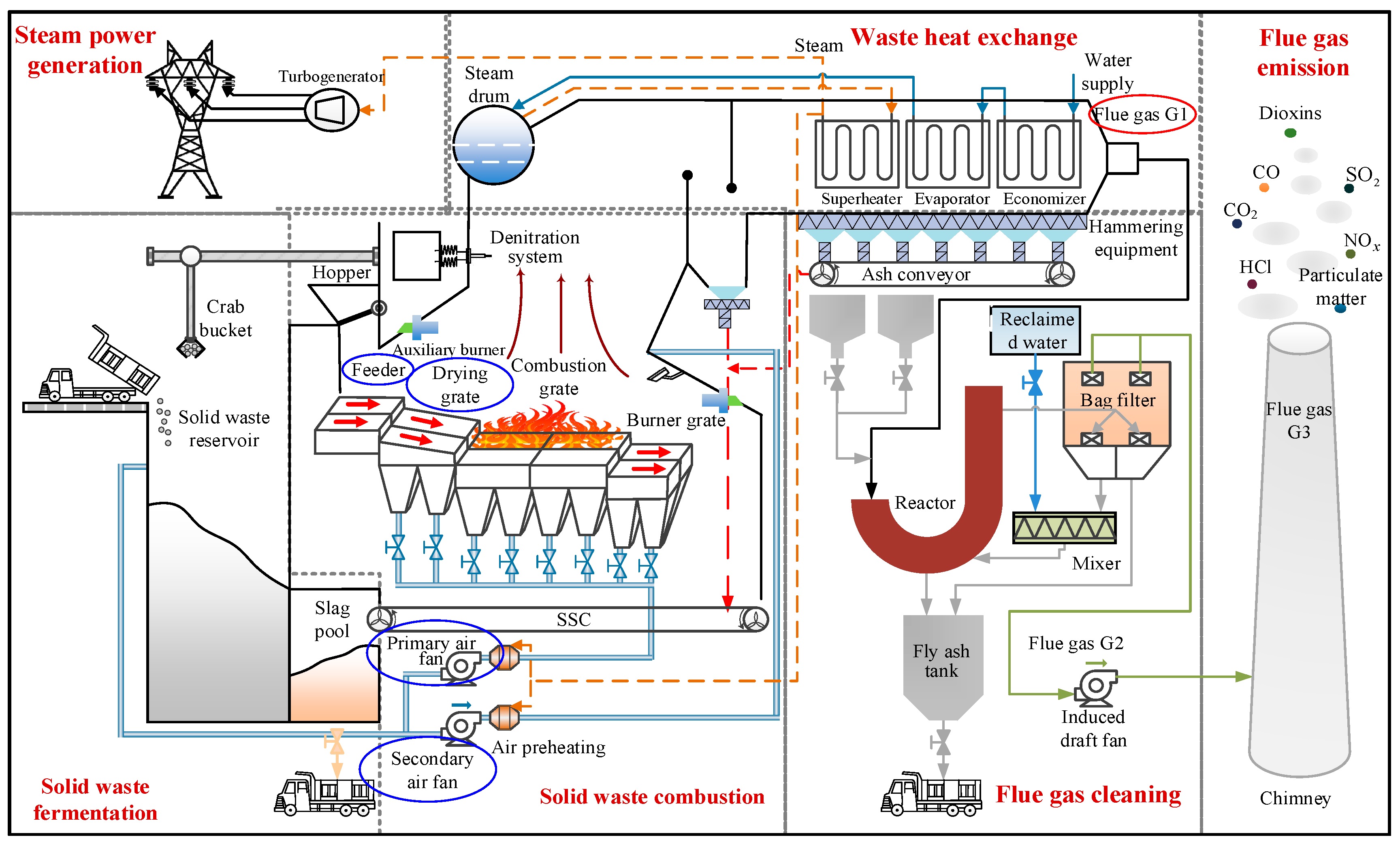
2.1.1. Municipal Solid Waste Incineration (MSWI) Process for Key Controlled Variables

This study is based on a typical MSWI plant with a grate furnace in Beijing. The process flow is shown in Figure 1.
The detailed descriptions of each element in Figure 1 are shown in Table A1. The red and blue circles are used to annotate the CVs and the MVs, respectively.
Figure 1 shows that this MSWI process mainly includes six stages: solid waste fermentation, solid waste combustion, waste heat exchange, flue gas cleaning, flue gas emission, and steam power generation. The detailed description is as follows.
  • Solid waste fermentation stage. The original MSW contains a significant amount of moisture, which hinders combustion. Therefore, it undergoes bio-fermentation in a solid waste reservoir. This process typically takes 5–7 days and increases the calorific value of the solid portion by approximately 30%. After fermentation, the MSW is transferred to the hopper and then pushed into the incinerator by the feeder, signaling the transition to the solid waste combustion stage.
  • Solid waste combustion stage. This stage involves converting MSW into high temperatures through the coupling interaction of multiple phases (solid, gas, liquid) and fields (heat, flow, force). It can be divided into three phases: drying, combustion, and burnout. The drying phase is achieved through the furnace’s heat radiation and the preheated primary air’s drying function. During the combustion phase, MSW is ignited, producing flue gas. After approximately 1.5 h of high-temperature combustion, the combustible components are fully burned, transitioning into the burnout phase. In this phase, non-combustible ash is pushed out of the furnace by the burnout grate.
  • Waste heat exchange stage. First, the high-temperature flue gas is initially cooled by the water wall. Next, heat energy is transferred to the boiler through radiation and convection via equipment such as superheaters, evaporators, and economizers. The water in the boiler is then converted into high-pressure superheated steam, entering the steam generation stage. Finally, the outlet flue gas temperature of the boiler is reduced to 200 °C. During this stage, it is crucial to strictly control the cooling rate to prevent the reformation of trace pollutants.
  • Steam power generation stage. This stage uses the high-temperature steam generated by the waste heat boiler to convert mechanical energy into electrical energy. This process achieves self-sufficiency in power consumption at the plant level and allows for the external supply of surplus power. In doing so, it facilitates resource utilization and generates economic benefits.
  • Flue gas cleaning stage. First, the denitrification system is employed to remove NOx. Next, the acid gases are neutralized using the semi-dry deacidification process. Then, activated carbon is used to adsorb DXN and heavy metals from the flue gas. Finally, the particles, neutralizing reactants, and activated carbon adsorbates in the flue gas are removed by the bag filter.
  • Flue gas emission stage. The flue gas that meets national emission standards is discharged into the atmosphere through the chimney, assisted by the induced draft fan.
The solid waste combustion stage is the most critical phase of the MSWI process, and its importance is reflected in several key aspects. First, it determines the steam flow generated during the waste heat exchange stage, which, in turn, influences the amount of electrical energy produced in the steam power generation stage and, ultimately, the total electricity generated by the MSWI power plant. Second, it impacts the degree of burnout of the MSW, directly affecting the amount of slag produced and the waste volume reduction rate. Finally, this stage assesses whether toxic pollutants in the flue gas can be effectively burned off, particularly in terms of pollutant concentration. The subsequent flue gas cleaning stage primarily focuses on reducing pollutant concentrations. Therefore, the lower the pollutant concentration at this stage, the less effort is required in the later stages of the flue gas cleaning process.
The key CVs involved in the solid waste combustion stage are furnace temperature, flue gas oxygen content, steam flow, and combustion line length. This stage consists of three sub-stages: drying, combustion, and burnout. During the combustion sub-stage, a strong oxidation reaction takes place, where the combustible components of the MSW react completely with oxygen. The flue gas oxygen content and MSW feed rate are critical to the combustion process. In the burnout sub-stage, the high temperature and primary air facilitate the oxidation of coke with oxygen. Therefore, maintaining stable flue gas oxygen content is crucial for the stable operation of the combustion process.

2.1.2. Detection Description of Flue Gas Oxygen Content

In the actual MSWI process, a zirconia oxygen sensor is used to measure the flue gas oxygen content. This sensor operates based on the ionic conductivity of oxygen, which is generated by stable zirconia ceramics at temperatures above 650 °C. At a given temperature, if there is an oxygen concentration difference between the inner and outer sides of the zirconium tube, a voltage is produced between the platinum electrodes. When the gas mixture is dilute, the oxygen content in the exhaust is high, resulting in a small oxygen concentration difference across the zirconium tube, and consequently, a low voltage output. However, when the gas mixture becomes more concentrated, the oxygen content in the exhaust decreases, and the concentrations of CO, CH, and NOx increase. These components react with the oxygen outside the zirconium tube, reducing the oxygen concentration on its outer surface to zero. As a result, the oxygen concentration difference between the inner and outer sides of the zirconium tube increases significantly, leading to a higher voltage output.

2.1.3. Importance of Flue Gas Oxygen Content Control in MSWI Process

In the MSWI process, flue gas oxygen content serves as an indicator of the excess air coefficient. The excess air coefficient is the ratio of the actual air volume to the theoretical air volume, reflecting the degree of excess oxygen supplied during combustion. It provides a measure of the combustion efficiency and can characterize the combustion state to some extent [4]. Two possible cases can arise:
  • Case 1: When the flue gas oxygen content is too low and the excess air coefficient is insufficient, it can lead to the production of a large amount of toxic and harmful gases. In addition, this condition results in increased heat loss and a decrease in combustion efficiency [14].
  • Case 2: When the flue gas oxygen content is too high and the excess air coefficient is too large, it indicates that the amount of air supplied is excessive. This excess air can carry away a significant amount of heat and dust. Additionally, high flue gas oxygen content can lead to an increase in the emission of NOx pollutants [14].
Normally, the flue gas oxygen content at the outlet of the waste heat boiler is considered one of the key CVs to monitor and optimize the MSWI process. Controlling the flue gas oxygen content within a specific range is essential for ensuring the complete combustion of MSW and combustible flue gases in the furnace. This, in turn, helps minimize the emission of secondary pollutants and ensures compliance with environmental standards. Therefore, developing an accurate model for controlling flue gas oxygen content is critical to optimizing the MSWI process and meeting environmental regulations [15].
The MSWI process is complex, with many variables influencing the flue gas oxygen content at the outlet of the waste heat boiler, some of which are interdependent. Therefore, the input features for modeling flue gas oxygen content are initially selected based on expert experience. These include primary air volume, secondary air volume, feeder speed average, drying grate speed average, and ammonia injection amount. A key challenge in developing such data-driven models is collecting process data for modeling without disrupting the normal operation of the industrial site.

2.2. Modeling Data Descripiton

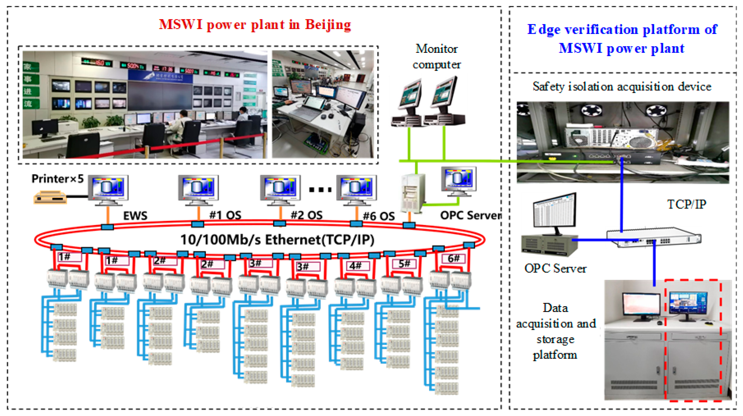
2.2.1. Data Acquisition Devices Description

To ensure the safe and reliable operation of the MSWI process, DCS systems with closed characteristics are strictly limited in their ability to connect with external devices for data collection and algorithm testing. As a result, we have designed a data acquisition system with a security isolation mechanism, which achieves absolute physical separation between the internal DCS system and the external data acquisition system through unidirectional optical fiber. However, this approach leads to additional equipment and personnel maintenance costs.
Data collection was conducted using an edge verification platform at an MSWI power plant, which is equipped with the safety isolation acquisition device mentioned earlier, as shown in Figure 2.
The device shown in Figure 2 enables one-way data transmission, helping to mitigate interference during the data acquisition process. The original industrial data used in this experiment were obtained with a 1 s sample period.

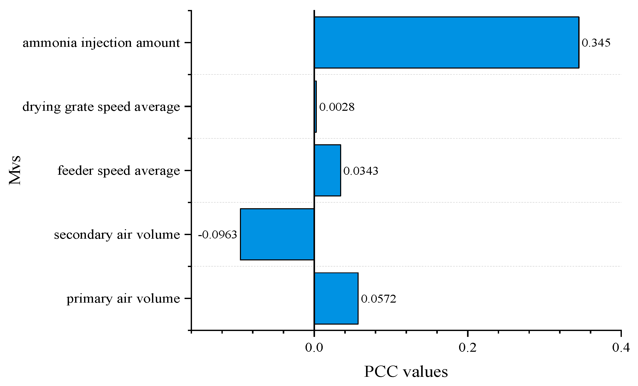
2.2.2. Experimental Data Analysis

This study used 16 h of continuous operation data with a sampling frequency of one sample per second from a certain MSWI power plant in Beijing on a specific day in March 2021. The data were averaged every 60 s, with outliers removed, resulting in a total of 857 samples. These processed data were then used to build the flue gas oxygen content control model. The samples were subsequently divided into training and testing sets in a 3:1 ratio.
The Pearson correlation coefficient (PCC) is a statistical measure used to assess the degree of linear correlation between each MV and flue gas oxygen content. Its value ranges from −1 to 1, where 1 indicates a perfect positive correlation, −1 indicates a perfect negative correlation, and 0 indicates no linear correlation. In this study, the PCC values between the key MVs and the CV are illustrated in Figure 3.
Figure 3 shows a significant linear correlation between the ammonia injection amount and flue gas oxygen content in the modeling data used in this study. However, the relationship between flue gas oxygen content and the key MVs may be more complex and nonlinear. Since the PCC can only capture linear relationships, Figure 3 does not reflect potential nonlinear or uncertain mappings. Therefore, when selecting MVs in practice, it is necessary to further consider on-site operational conditions, such as airflow distribution and material allocation.
In terms of the optimal control range for flue gas oxygen content, Sun et al. [17] found that under specific operating conditions, a range of 5 to 6.5 is effective. We extended the control range in this study, proposing an optimal flue gas oxygen content range of 6 to 8 under different operating conditions.
It is important to note that we are currently developing and testing the algorithm using industrial process data, with the aim of applying it to real-world industrial processes in future research.

2.3. Method

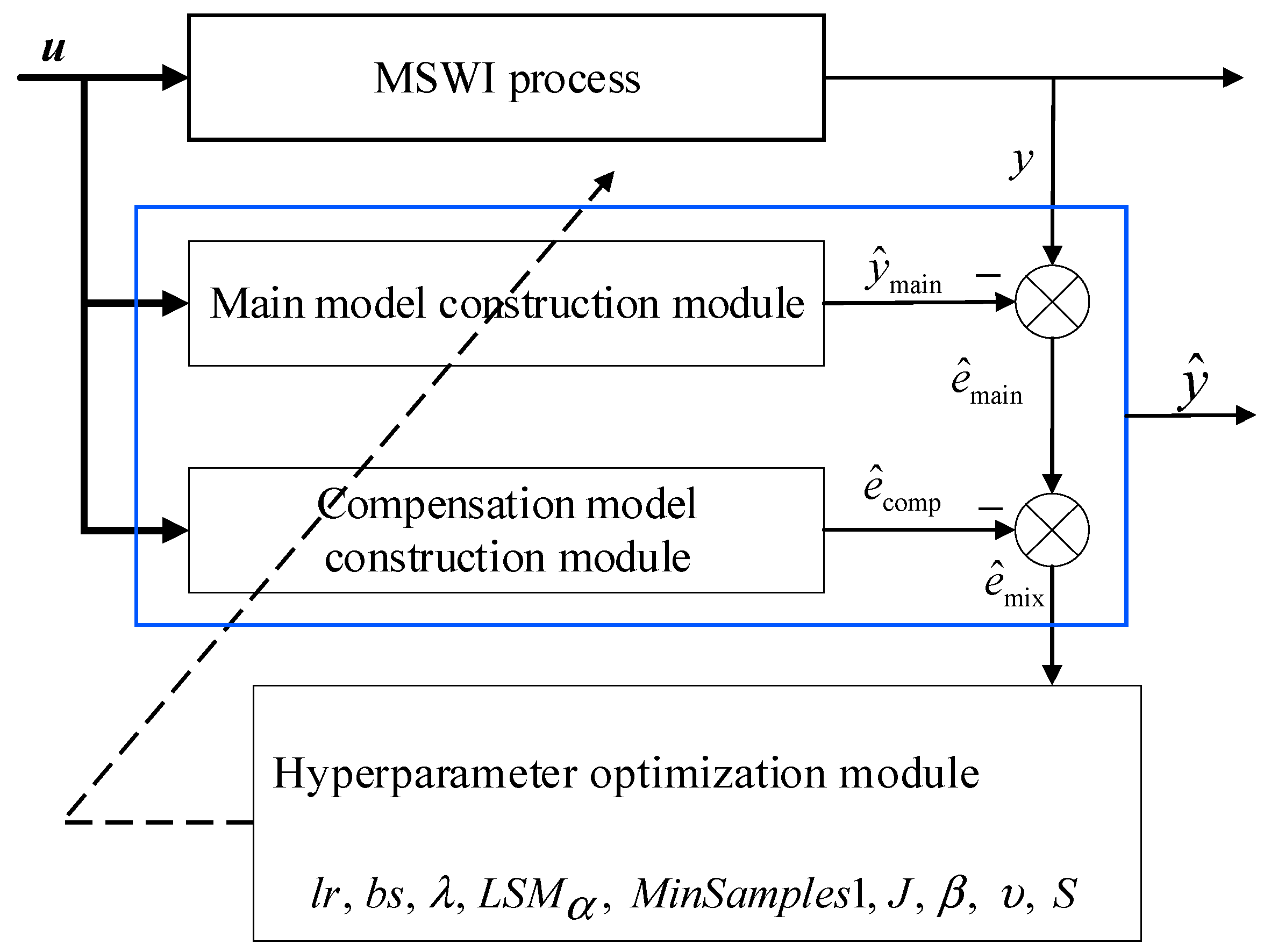
2.3.1. Main–Compensation Ensemble Modeling Strategy

An interpretable flue gas oxygen content model based on BO-EnTSFRT-LSTM is proposed. In this model, EnTSFRT is used to construct the main model to capture uncertainty, LSTM is employed to build a compensation model using the main model’s error as the true value, and the BO algorithm is applied to optimize the hyperparameters of the main–compensation ensemble model. The overall modeling strategy is illustrated in Figure 4.
In Figure 4, u denotes input variables (MVs); y and y ^ represent the true value and the model output value of flue gas oxygen content; y ^ main represents the output value of the main model; e ^ main and e ^ mix represent the error values of the main model and the compensation model; e ^ comp denotes the output value of the compensation model; l r , b s , λ , L S M α , M i n S a m p l e s 1 , and J are learning rate, number of batches, the initial value of the intermediate variable in the recursive calculation process, regularization coefficient, the minimum number of samples, and the number of sub-models for the main model; β , υ , and S are the learning rate, regularization coefficient, and maximum number of iterations for the compensation model.
The relationships among e ^ main , y , y ^ , y ^ main , and e ^ comp are as follows:
e ^ main = y y ^ main
y ^ = y ^ main + e ^ comp
The functions of different modules are as follows:
(1) Main model construction module: It constructs the main model by creating multiple TSFRT sub-models using a parallel fusion mode.
(2) Compensation model construction module: It constructs the compensation model with the error of the main model as the true value by using LSTM.
(3) Hyperparameter optimization module: The hyperparameters of the main–compensation ensemble model are optimized based on the module.
Remark 1.
The steps of the modeling strategy are as follows. Firstly, u is used as the input of the main model to obtain the predicted value of flue gas oxygen content. Secondly, the model error is calculated, and the LSTM model is constructed based on this error. Then, the BO algorithm is applied to optimize the hyperparameters of the main–compensation model, enabling accurate modeling of the flue gas oxygen content. Finally, the final predicted value of the flue gas oxygen content is obtained.

2.3.2. Modeling Algorithm Implementation

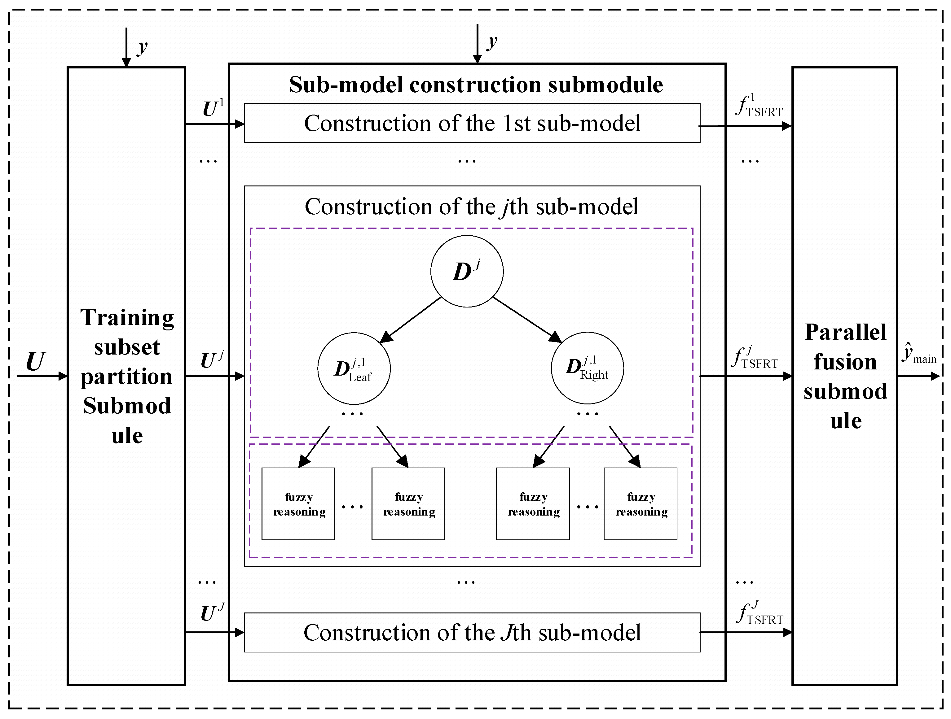
Main Model Construction Module

The structure of the main model based on EnTSFRT is shown in Figure 5.
In Figure 5, U and y represent the input matrix and output vector of the training subset, respectively; U j represents the input matrix of the j th training subset; j = 1 , 2 , , J represents the index of the training subset; J represents the number of training subsets; D = U , y = u n , y n n = 1 N N × M denotes the modeling data set; n = 1 , 2 , , N generally represents the index of the sample; N represents the total number of input samples; M ( m = 1 , 2 , , M ) represents dimensions of the input feature; u n denotes the n th input sample in D ; y n represents the true value of the n th sample in D ; D j denotes the j th training subset obtained by performing random sampling with the Bootstrap method on D ; D Left j , 1 and D Right j , 1 denote the left subset and right subset obtained by splitting the first non-leaf node, respectively.
The EnTSFRT model consists of multiple TSFRT sub-models with a parallel fusion structure. Each TSFRT sub-model includes a screening layer and a fuzzy reasoning layer. The screening layer is responsible for feature selection, while the fuzzy reasoning layer applies TS fuzzy reasoning. The details are as follows.
(1)
Training subsets’ partition sub-module.
The training subset D j containing M features can be expressed as follows:
D j = u n j , y n j n = 1 N = U j , y j N × M , j = 1 , 2 , , J
where y j = y n j n = 1 N represents the true value vector of flue gas oxygen content.
Correspondingly, from the perspective of input features, u n j can be expressed as follows:
u n j = [ u n , 1 j , , u n , m j , , u n , M j ] 1 × M
Therefore, D 1 , , D j , D J can be obtained.
(2)
Sub-model construction sub-module.
The construction of the j th TSFRT sub-model is described as an example.
Assume the j th TSFRT sub-model consists of M j nodes. The number of non-leaf nodes is calculated as M nonleaf j = M j 2 1 ( m nonleaf j = 1 , 2 , , M nonleaf j ), and the number of leaf nodes is denoted as M leaf j ( m leaf j = 1 , 2 , , M leaf j ). The following relationships hold:
M j = M nonleaf j + M leaf j
The training subset D j is used as the input of the screening layer. Each recursive coordinate point n , m in D j is obtained and its mean square error (MSE) value is calculated. The segmentation nodes are determined by minimizing MSE. The estimation process of the loss function value is denoted as follows:
Φ = arg min n , m f MSE m nonleaf j D Left j , m nonleaf j + f MSE m nonleaf j D Right j , m nonleaf j = arg min n , m y Left j , m nonleaf j ϑ Left j , m nonleaf j μ c s j , m nonleaf j u n j 2 + y Right j , m nonleaf j ϑ Right j , m nonleaf j μ c s j , m nonleaf j u n j 2
where Φ represents the minimum loss value when the split point is n , m ; D Left j , m nonleaf j and D Right j , m nonleaf j represent the left subset and right subset of the m nonleaf j th non-leaf node in the j th TSFRT sub-model; f MSE m nonleaf j denotes the MSE value of the left subset D Left j , m nonleaf j ( D Right j , m nonleaf j ); y Left j , m nonleaf j and y Right j , m nonleaf j represent the true vectors of the left subset D Left j , m nonleaf j and right subset D Right j , m nonleaf j ; μ c s j , m nonleaf j denotes the clear membership function of input at the m nonleaf j th non-leaf node; ϑ Left j , m nonleaf j and ϑ Right j , m nonleaf j represent the average of the target values of the left subset D Left j , m nonleaf j and the right subset D Right j , m nonleaf j .
In this article, both ϑ Left j , m nonleaf j and ϑ Right j , m nonleaf j are represented as ϑ m nonleaf j j . Its calculation is as follows:
ϑ m nonleaf j j = 1 N j , m nonleaf j n = 1 N j , m nonleaf j y n j
where N j , m nonleaf j denotes the number of samples in the D Left j , m nonleaf j ( D Right j , m nonleaf j ).
In Equation (6), μ c s j , m nonleaf j u n j is calculated as follows:
μ c s j , m nonleaf j u n j = 1   if   u n , m j ϕ m nonleaf j j 0   if   u n , m j < ϕ m nonleaf j j
where ϕ m nonleaf j j indicates the segmentation threshold at the m nonleaf j th non-leaf node, and it can be expressed as ϕ m nonleaf j j = u n , m j .
Therefore, the membership set is μ CS j , m nonleaf j ( ) m nonleaf j = 1 M nonleaf j .
It is assumed the clear set at the m leaf j th leaf node is C cs j , m leaf j . By looping through all feature values to complete the first data set split and obtaining the first element ϕ 1 j in C cs j , m leaf j , the initial clear set C cs _ 1 j , m leaf j at the m leaf j th leaf node is described as follows:
C cs _ 1 j , m leaf j : ϕ 1 j
D j is divided into left and right subsets as follows:
D Left j , m nonleaf j : D Left j , m nonleaf j N Left j , m nonleaf j × M | μ c s j , m nonleaf j u n j 1 D Right j , m nonleaf j : D Right j , m nonleaf j N Right j , m nonleaf j × M | μ c s j , m nonleaf j u n j 0
where N Left j , m nonleaf j and N Right j , m nonleaf j represent the number of samples in the D Left j , m nonleaf j and D Right j , m nonleaf j , respectively. If the membership degree of sample u n j is 1, it belongs to the left subset; if it is 0, it belongs to the right subset.
By repeating the above steps until the minimum number of samples at the leaf node reaches the set threshold, set D j , m leaf j m leaf j = 1 M leaf j with M leaf j subsets is obtained.
At the same time, the clear set C cs j , m leaf j of the m leaf j th leaf node can be expressed as follows:
C cs j , m leaf j : ϕ 1 j , , ϕ m nonleaf j j , , ϕ M nonleaf j j
The input of the fuzzy reasoning layer corresponding to the m leaf j th leaf node is denoted as D fuzzy j , m leaf j . The D fuzzy j , m leaf j is represented as follows:
D fuzzy j , m leaf j = u n j , m leaf j j , m leaf j C cs m leaf j , y n j , m leaf j j , m leaf j n j , m leaf j = 1 N j , m leaf j N j , m leaf j × M nonleaf j + 1
where u n j , m leaf j j , m leaf j = u n j , m leaf j , 1 j , m leaf j , , u n j , m leaf j , m nonleaf j j , m leaf j , , u n j , m leaf j , M nonleaf j j , m leaf j represents the n j , m leaf j th input vector of the m leaf j th fuzzy reasoning layer, u n j , m leaf j , m nonleaf j j , m leaf j denotes the m nonleaf j th feature of n j , m leaf j th input vector of the m leaf j th fuzzy reasoning layer; N j , m leaf j denotes the number of samples in the m leaf j th leaf node.
In the fuzzy reasoning layer, K k = 1 , 2 , , K rules are defined to represent the local linear relationship between the input variable and the output. We define the k th rule as follows:
R u l e k : i f   u n j , m leaf j , 1 j , m leaf j   i s   μ A n j , m leaf j , 1 j , k j u n j , m leaf j , 1 j , m leaf j     and   u n j , m leaf j , M nonleaf j j , m leaf j   is   μ A n j , m leaf j , m nonleaf j j , k j u n j , m leaf j , m nonleaf j j , m leaf j   and   u n j , m leaf j , M nonleaf j j , m leaf j   is   μ A n j , m leaf j , M nonleaf j j , k j u n j , m leaf j , M nonleaf j j , m leaf j , t h e n   y j , k = g j , k u n j , m leaf j , 1 j , m leaf j , , u n j , m leaf j , m nonleaf j j , m leaf j , , u n j , m leaf j , M nonleaf j j , m leaf j
where μ A n j , m leaf j , m nonleaf j k j represents the membership degree of u n j , m leaf j , m nonleaf j j , m leaf j belonging to A n j , m leaf j , m nonleaf j j , k , y j , k represents the output of the k th fuzzy rule, and the function g j , k u n j , m leaf j , 1 j , m leaf j , , u n j , m leaf j , m nonleaf j j , m leaf j , , u n j , m leaf j , M nonleaf j j , m leaf j represents the linear combination of the outputs, and it can be represented as follows:
g j , k u n j , m leaf j , 1 j , m leaf j , , u n j , m leaf j , m nonleaf j j , m leaf j , , u n j , m leaf j , M nonleaf j j , m leaf j = ω 1 j , k u n j , m leaf j , 1 j , m leaf j + + ω m nonleaf j j , k u n j , m leaf j , m nonleaf j j , m leaf j + + ω M nonleaf j j , k u n j , m leaf j , M nonleaf j j , m leaf j
where ω j , k = ω 1 j , k , , ω m nonleaf j j , k , , ω M nonleaf j j , k denotes the weight of the consequent part of the k th rule, and ω m nonleaf j j , k represents the weight of the input variable u n j , m leaf j , m nonleaf j j , m leaf j .
In the article, the Gaussian function is used as a membership function, as follows:
μ A n j , m leaf j , m nonleaf j j , k j u n j , m leaf j , m nonleaf j j , m leaf j = exp u n j , m leaf j , m nonleaf j j , m leaf j δ n j , m leaf j , m nonleaf j j , k 2 σ n j , m leaf j , m nonleaf j j , k 2
where δ n j , m leaf j , m nonleaf j j , k denotes the center of the membership function μ A n j , m leaf j , m nonleaf j j , k j , and σ n j , m leaf j , m nonleaf j j , k represents the width of membership function μ A n j , m leaf j , m nonleaf j j , k j .
The activation intensity of the k th fuzzy rule represents the product of the membership degrees of the input variables in each fuzzy set, and is calculated as follows:
α j , k = min μ A n j , m leaf j , 1 j , k j u n j , m leaf j , 1 j , m leaf j , , μ A n j , m leaf j , M nonleaf j j , k j u n j , m leaf j , M nonleaf j j , m leaf j
where α j , k denotes the activation intensity of the k th fuzzy rule, and m nonleaf j = 1 M nonleaf j represents the Cartesian product.
Furthermore, the normalization operation is performed as follows:
α ¯ j , k = α j , k k = 1 K α j , k
According to Equations (13)–(17), y j , k and α ¯ j , k are linearly combined and accumulated. The predicted output values can be obtained as follows:
y ^ n j , m leaf j j , m leaf j = k = 1 K α ¯ j , k g j , k u n j , m leaf j j , m leaf j = k = 1 K α j , k k = 1 K α j , k ω 1 j , k u n j , m leaf j , 1 j , m leaf j + + ω m nonleaf j j , k u n j , m leaf j , m nonleaf j j , m leaf j + + ω M nonleaf j j , k u n j , m leaf j , M nonleaf j j , m leaf j
For the membership functions in the antecedent part, the center δ is initialized using a standard normal distribution with a mean of 0 and a standard deviation of 1, while the width σ is initialized using a uniform distribution in the range of [10, 10]. These hyperparameters are updated using the backpropagation algorithm.
The weight ω j , k = ω 1 j , k , , ω m nonleaf j j , k , , ω M nonleaf j j , k in the consequent part is updated using a strategy based on prior knowledge for initializing the weights. Combining Equation (6), we obtain a set of loss function values, denoted as Φ back = Φ 1 back , , Φ m nonleaf j back , , Φ M nonleaf j back . They are then normalized to initialize the weights of the consequent parts, as shown below:
ω 0 j , k = Φ m nonleaf j back m nonleaf j = 1 M nonleaf j Φ m nonleaf j back
where ω 0 j , k is the weight of the initial time, and Φ m nonleaf j back denotes the m nonleaf j th value in Φ back .
The recursive calculation of ω j , k is as follows:
H n j , m leaf j + 1 j = H n j , m leaf j j H n j , m leaf j j ω n j , m leaf j j , k u n j , m leaf j j , m leaf j T ω n j , m leaf j j , k u n j , m leaf j j , m leaf j H n j , m leaf j j 1 + ω n j , m leaf j j , k u n j , m leaf j j , m leaf j T H n j , m leaf j j ω n j , m leaf j j , k u n j , m leaf j j , m leaf j
ω n j , m leaf j + 1 j , k = ω n j , m leaf j j , k + H n j , m leaf j + 1 j ω n j , m leaf j j , k u n j , m leaf j j , m leaf j T y n j , m leaf j j , m leaf j ω n j , m leaf j j , m leaf j ω n j , m leaf j j , m leaf j u n j , m leaf j j , m leaf j T T
where H n j , m leaf j j is the intermediate variable in the recursive process; H 0 j is defined by H 0 j = λ I ; λ is a large positive value; and I represents the unit matrix. The purpose of Equation (20) is to update the error correction factor in order to adjust the response to new data in subsequent calculations. Equation (21) uses the error information from the new data to adjust the weights ω n j , m leaf j + 1 j , k , so that the predicted values are closer to the true values.
Thus, the construction of the j th TSFRT sub-model is completed. The simplified multi-input single-output TSFRT sub-model can be obtained as follows:
y ^ main j = f TSFRT j U j
(3)
Parallel fusion sub-module
According to the modeling process of TSFRT, the constructed total TSFRT sub-models are denoted as f TSFRT j j = 1 J . The prediction outputs of these sub-models with N samples are denoted as F N × J .
To estimate the weights with the minimum training error of the parallel fusion sub-module, the following optimal problem is to be solved:
arg min W LSM J : F W LSM J y 2 + L S M α W LSM J 2
Using ridge regression theory, specifically the Moore–Penrose inverse matrix, the weight matrix is calculated. The results are given by the following equation:
W LSM J = F T L S M α I + F F T 1 y
The output of EnTSFRT is denoted as follows:
y ^ main = F W LSM J = f TSFRT j U j j = 1 J W LSM J

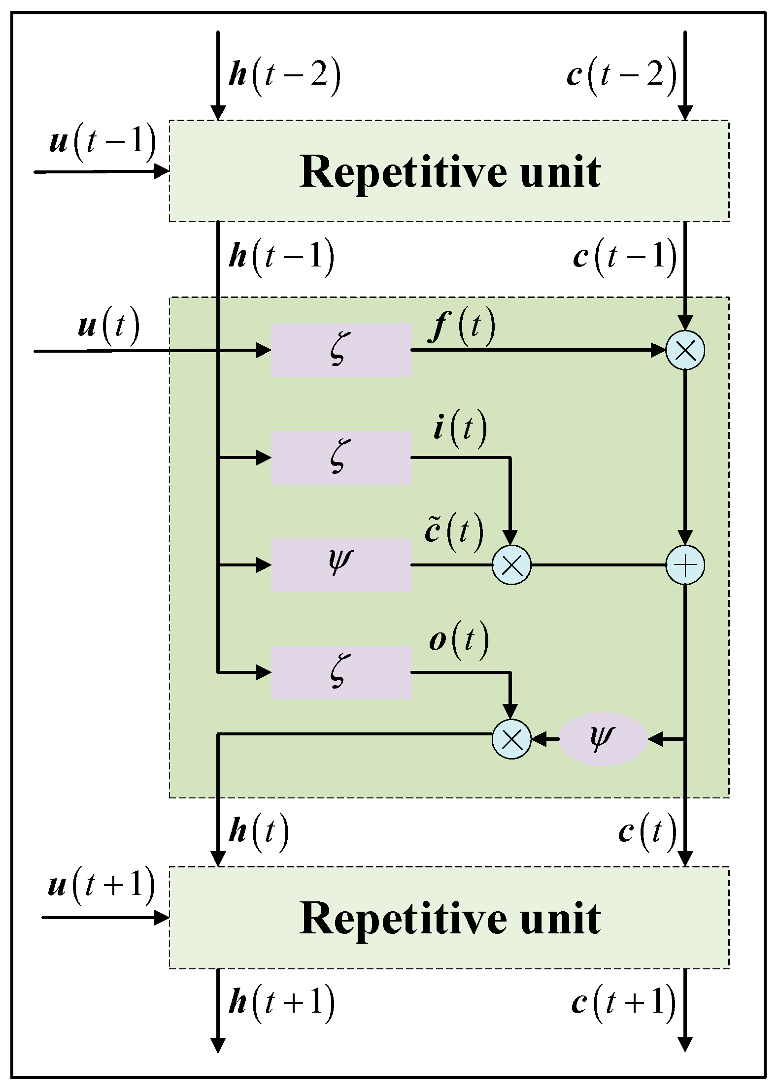
Compensation Model Construction Module

The structure of the compensation model based on LSTM is shown in Figure 6.
In Figure 6, t denotes the current moment, h denotes the hidden state, c denotes the cell state, c ˜ denotes the candidate cell state, ζ represents the sigmoid function, ψ represents the tanh function, f denotes the value of the forget gate, i denotes the value of the input gate, o represents the value of the output gate, and represents element-by-element multiplication.
(1)
Forward calculation process
The input of the compensation model is denoted as D E = u t , e ^ main t N × M . The forward calculation process at time t is described as follows.
Firstly, the output of the forget gate is updated as follows:
f t = ζ W uf u t + W hf h t 1 + b f
where W uf and W hf represent the weight matrix; b f represents the bias matrix.
Secondly, the output of the input gate is updated, and a new candidate cell state is generated, as follows:
i t = ζ W ui u t + W hi h t 1 + b i
c ˜ t = ψ W u c ˜ u t + W h c ˜ h t 1 + b c ˜
Furthermore, the cell state is updated as follows:
c t = c t 1 f t + c ˜ t i t
Then, the output gate is updated and the cell state at t is generated, as follows:
o t = ζ W uo u t + W ho h t 1 + b o
h t = o t ψ c t
Finally, the output value e ^ comp t of LSTM is obtained as follows:
e ^ comp t = W out h t
where W out is the output weight matrix.
(2)
Backpropagation process
The loss function J t i of LSTM is defined as follows:
J t = 1 2 e ^ main t e ^ comp t 2
The weights and biases are updated based on the backpropagation algorithm. Taking the update of W uf as an example, it is shown as follows:
W uf t + 1 = W uf t β J t W uf t
Using the chain rule, J t W uf is calculated as follows:
J t W uf t = J t e ^ comp t e ^ comp t W uf t = e ^ main t e ^ comp t e ^ comp t W uf t
The calculation of e ^ comp t W uf t is shown as follows:
e ^ comp t W uf t = e ^ comp t h t h t c t c t f t f t W uf t = υ out o t sech 2 c t c t 1 f t 1 f t u t
Further, W uf t + 1 can be obtained.
The update process of the remaining weights and biases is the same as the update process of W uf .

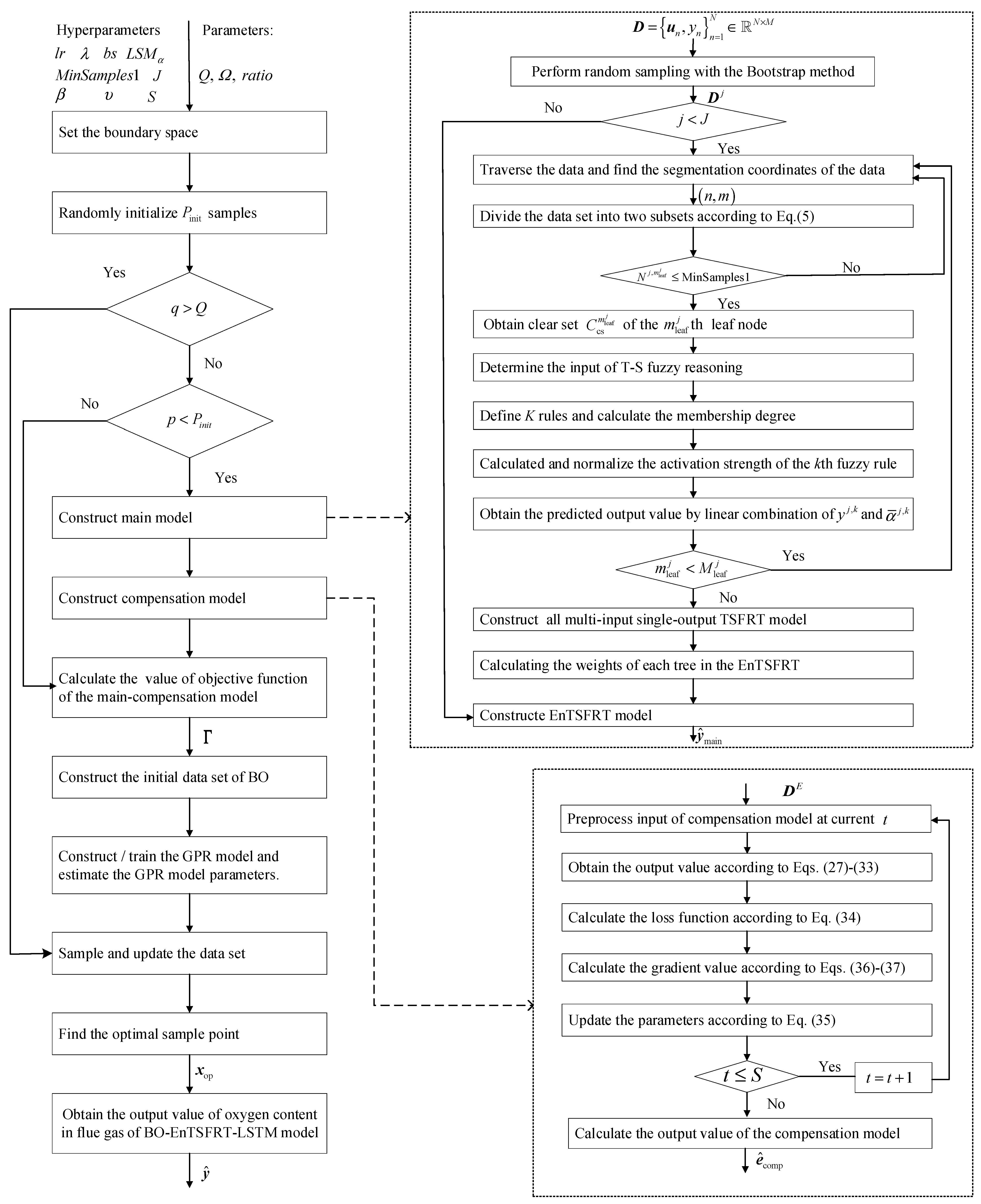
Hyperparameter Optimization Module

The BO algorithm is used to select the nine hyperparameters in the main–compensation ensemble model to minimize the objective function. In this article, the objective function chosen is the negative value of the R-squared (R2) indicator. The optimization process of BO algorithm is described as follows.
(1)
Set the boundary space.
We set the value range for the hyperparameters of the main–compensation ensemble model, which includes the upper boundary (UB) and the lower boundary (LB) of the sample space, defined as follows:
LB 1 < x 1 < UB 1 LB 9 < x 9 < UB 9
where x 1 , , x 9 denotes the following:
x 1 l r x 2 λ x 3 b s x 4 L S M α x 5 M i n S a m p l e s 1 x 6 J x 7 β x 8 υ x 9 S
(2)
Construct the initial data set.
We randomly initialize input samples with a number P init , and the corresponding set of objective function values is denoted as Γ = Γ x 1 , , Γ x P init T . This forms the initial data set.
(3)
Construct/train the GPR model.
The Gaussian process regression (GPR) model is constructed using this data set. Since the GPR model treats the known data as a prior probability distribution that follows a multivariate normal distribution, it is expressed as follows:
Γ ~ N ξ 0 , Σ 0
where ξ 0 = [ ξ 0 ( x 1 ) , , ζ 0 ( x p ) ] represents the mean function, p denotes the number of data set samples at the current time, and Σ 0 denotes the covariance matrix as follows:
Σ 0 = Σ 0 ( x 1 , x 1 ) Σ 0 ( x 1 , x p ) Σ 0 ( x p , x 1 ) Σ 0 ( x p , x p ) + σ 2 I p × p
where σ 2 represents the variance of the measurement noise, and Σ 0 ( x a , x b ) denotes the kernel function between the a th and b th sample points, which is calculated as follows:
Σ 0 ( x a , x b ) = σ Γ 2 exp ( 1 2 ο = 1 d x a o x b o 2 η o 2 )
where x a o represents the o th dimension feature of the a th sample, σ Γ is the kernel amplitude of the kernel function, and η o denotes the length ratio of the o th dimension of the sample.
For a new sample point in the sample space, the posterior probability distribution of the sample point can be calculated based on the prior probability distribution. According to the definition of GP, the joint Gaussian distribution Γ and the predicted value Γ ^ * of the known data also follow the Gaussian distribution, which can be expressed as follows:
Γ Γ ^ * N 0 , Σ 0 Σ 0 Σ 0 T Σ 0
where Σ 0 = Σ 0 ( x 1 , x 1 ) , , Σ 0 ( x p , x ) T p × 1 represents the covariance of the training testing set, and Σ 0 = Σ 0 ( x , x ) 1 × 1 denotes the covariance of the testing set.
Since the training set is known, the conditional distribution of Γ ^ * for a given Γ can be calculated based on Equation (42) as follows:
Γ ^ * | Γ N ζ p , σ p 2
where ξ p and σ p 2 are as follows:
ξ p = Σ 0 T Σ 0 1 Γ ξ 0 + ξ 0 x σ p 2 = Σ 0 Σ 0 T Σ 0 1 Σ 0
where ξ p is the posterior mean value, and σ p 2 denotes the posterior variance.
(4)
Estimate the parameters of the GPR model.
We estimate the parameters of the mean function and covariance matrix using maximum likelihood estimation (MLE).
(5)
Sampling.
In order to find the optimal point x op that minimizes the objective function value Γ x op , the expected improvement (EI) sampling function is used to sample the objective function.
(6)
Update the data set.
We calculate the objective function value Γ x corresponding to the new sample point x . Then, the data sets X = x 1 ; ; x p ; x and Γ = Γ x 1 , , Γ x p , Γ x T are updated.
The steps (3) to (6) are repeated until the preset maximum number of iterations is reached. Afterward, the optimal sample point x op that meets the requirements is identified from the data set.

2.3.3. Pseudocode and Flow Chart

Pseudocode

The pseudocode for the BO-EnTSFRT-LSTM algorithm is as follows.
Algorithm 1 shows that the parameters of the BO process are Q , Ω , and r a t i o . Among them, BO establishes a probability model based on the past evaluation results of the objective function to find the value that minimizes the objective function. Commonly used sampling functions include expectation boosting, knowledge gradient, and entropy search and predictive entropy search. The selection of a sampling function needs to consider how likely it is to obtain the optimal value at a given point and to evaluate whether the point can reduce the uncertainty of the Bayesian statistical model. The exploration ratio is a parameter that controls the balance between exploration and exploitation, and it needs to be adjusted according to specific optimization tasks and application scenarios.
Algorithm 1. Pseudocode of the BO-EnTSFRT-LSTM algorithm.
1Data set D ; Parameters of BO: Q , Ω , r a t i o ; Hyperparameters of EnTSFRT: l r , λ , b s , L S M α , M i n S a m p l e s 1 and J ; Hyperparameters of LSTM: β , υ and S
Output: Predicted value y ^
2Read the data, set the boundary space, and randomly initialize P init samples;
3If q < Q
4 If p < P i n i t
5  Take D = u n , y n n = 1 N N × M as the input of the EnTSFRT model;
6  If j < J
7   If m leaf j < M leaf j
8    If N j , m leaf j MinSamples 1
9     Traverse the data and determine the optimal segmentation point by minimizing the MSE;
10     Divide the data into two subsets, D Left j , m leaf j and D Right j , m leaf j ;
11    end
12    Obtain subsets D j , m leaf j m leaf j = 1 M leaf j , and the clear set C cs j , m leaf j of the m leaf j th leaf node;
13    Obain the input of the fuzzy reasoning layer corresponding to the m leaf j th leaf node D fuzzy j , m leaf j ;
14    Define K rules to represent the local linear relationship between the input variable and the output;
15    Calculate the membership degree of u n , m nonleaf j j , m leaf j to A n , m nonleaf j j , k ;
16    Calculate the activation intensity α j , k of the kth fuzzy rule and carry out the normalization operation to obtain α ¯ j , k ;
17    Obtain the predicted output value y ^ n j , m leaf j j , m leaf j by linear combination of y j , k and α ¯ j , k ;
18   end
19   Construct a multi-input single-output TSFRT sub-model f TSFRT j ;
20   Update the weights of consequent.
21  end
22  Construct EnTSFRT by ensemble multiple TSFRT sub-models;
23  Calculate the error value of the EnTSFRT model;
24  Use D E as the input of LSTM model;
25  Initialize the parameters;
26  If s S
27   Calculation the outputs according to Equations (26)–(32);
28   Calculate the loss function according to Equation (33);
29   Calculate the gradient value according to Equations (35) and (36);
30   Update the parameters according to Equation (34);
31  end
32 end
33 Construct BO initial data set;
34 Construct GPR model;
35 Sample and update the data set;
36 Find the optimal sample point;
37end
38Obtain the predicted value y ^ .

Flow Chart

The flow chart of the BO-EnTSFRT-LSTM algorithm is shown in Figure 7.
In Figure 7, Q ( q = 1 , 2 , , Q ) denotes the number of iterations of the optimization process, Ω denotes the EI sampling function, and r a t i o denotes the exploration ratio.

3. Results and Discussion

3.1. Evaluation Indices

The evaluation indices used in the article are root mean squared error (RMSE), mean absolute error (MAE), and R-squared (R2), as follows:
R M S E = n = 1 N y n y ^ n 2 N
M A E = 1 N n = 1 N y ^ n y n
R 2 = 1 n y ^ n y n 2 n y ¯ n y n 2
Among the three indices, RMSE represents the standard deviation of the differences between the predicted value and the true value, reflecting the degree of dispersion in the sample. In nonlinear fitting, a smaller RMSE indicates better performance. MAE represents the average absolute error between the predicted value and the true value. R2 quantifies how well the model fits the data, with a value closer to 1 indicating a better fit.

3.2. Experimental Results

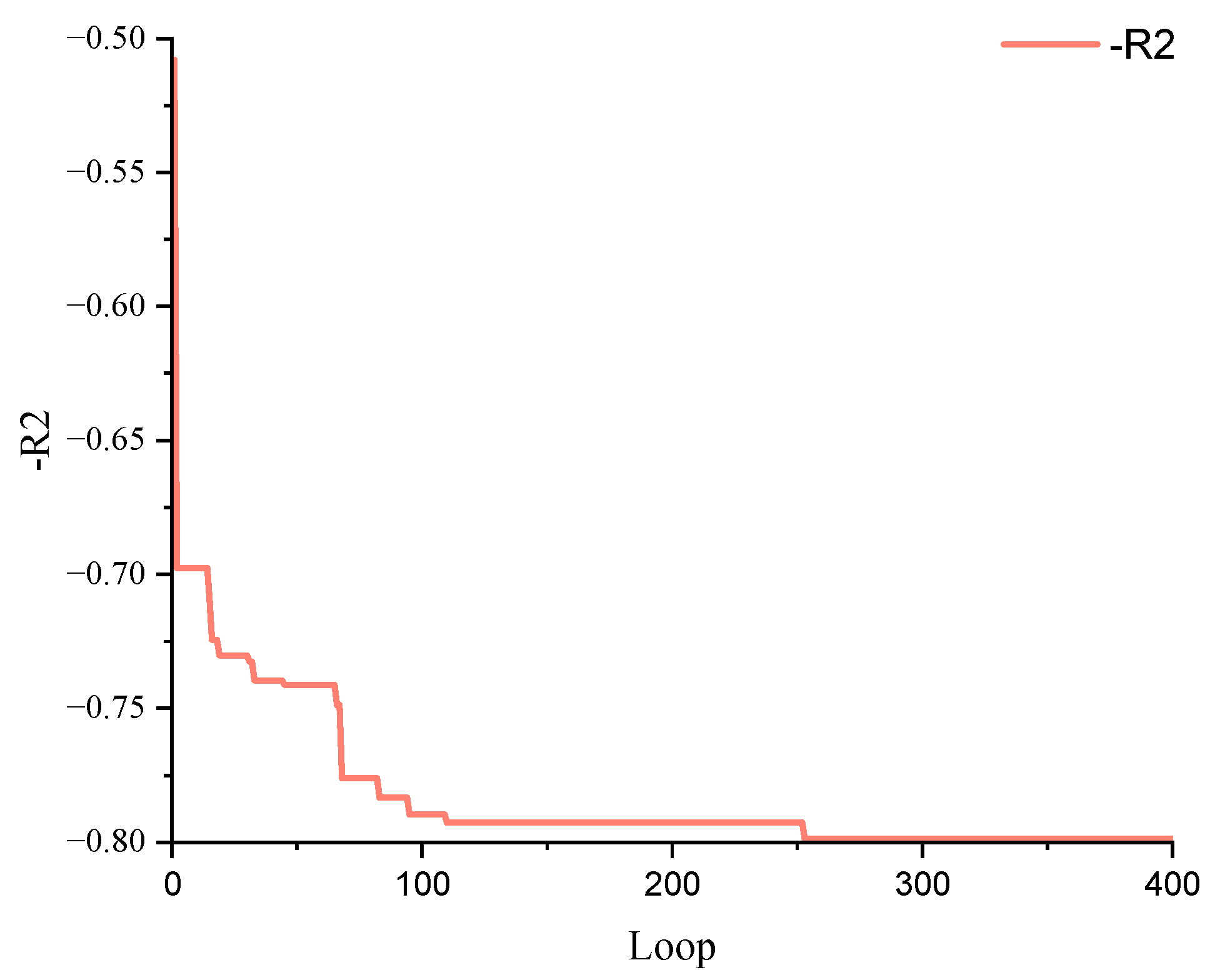
3.2.1. BO Parameters Based on the Grid Search

The BO parameters were selected using the grid search method. The selection process involves defining the parameter grid, generating parameter combinations, performing cross-validation for each combination, and then selecting the best BO parameters. The details are as follows.
(1) Define the parameter grid: The BO parameters and their corresponding value ranges are as follows: the number of optimization iterations [100, 200, 400, 800], the exploration ratio [0.1, 0.3, 0.5, 0.7, 0.9], and the acquisition function [“expected-improvement”, “probability-of-improvement”, “lower-confidence-bound”].
(2) Generate parameter combinations: We generate all possible permutations and combinations of the hyperparameters to create a parameter grid. Based on the BO parameters mentioned above, the total number of combinations is 4 × 5 × 3 = 60.
(3) Perform cross-validation for each combination: We split the data set in a 3:1 ratio into a training set and a validation set, with the training set used to train the model and the validation set used to evaluate its performance.
(4) Select the best BO parameters: By comparing the validation results of all combinations, we select the parameter combination that yields the best performance.
In this article, the first combination is evaluated with a specific number of optimization iterations Q = 100 , r a t i o = 0.1 , and Ω = expected - improvement , and the R2 evaluation metric is 0.75158. Using the same method, the other 59 combinations were also assessed. Ultimately, when the parameters are set to Q = 400 , r a t i o = 0.5 , and Ω = expected - improvement , the R2 reaches its maximum value of 0.79876, indicating that this hyperparameter combination is the optimal one
The detailed values are Q = 400 , Ω = EI function, and r a t i o = 0.5. The optimal hyperparameters of main–compensation ensemble model are selected as l r = 0.1829 , λ = 23 , b s = 21 , L S M α = 0.6714 , M i n S a m p l e s 1 = 42 , J = 23 , β = 0.0263 , υ = 0.1923 , and S = 345 .

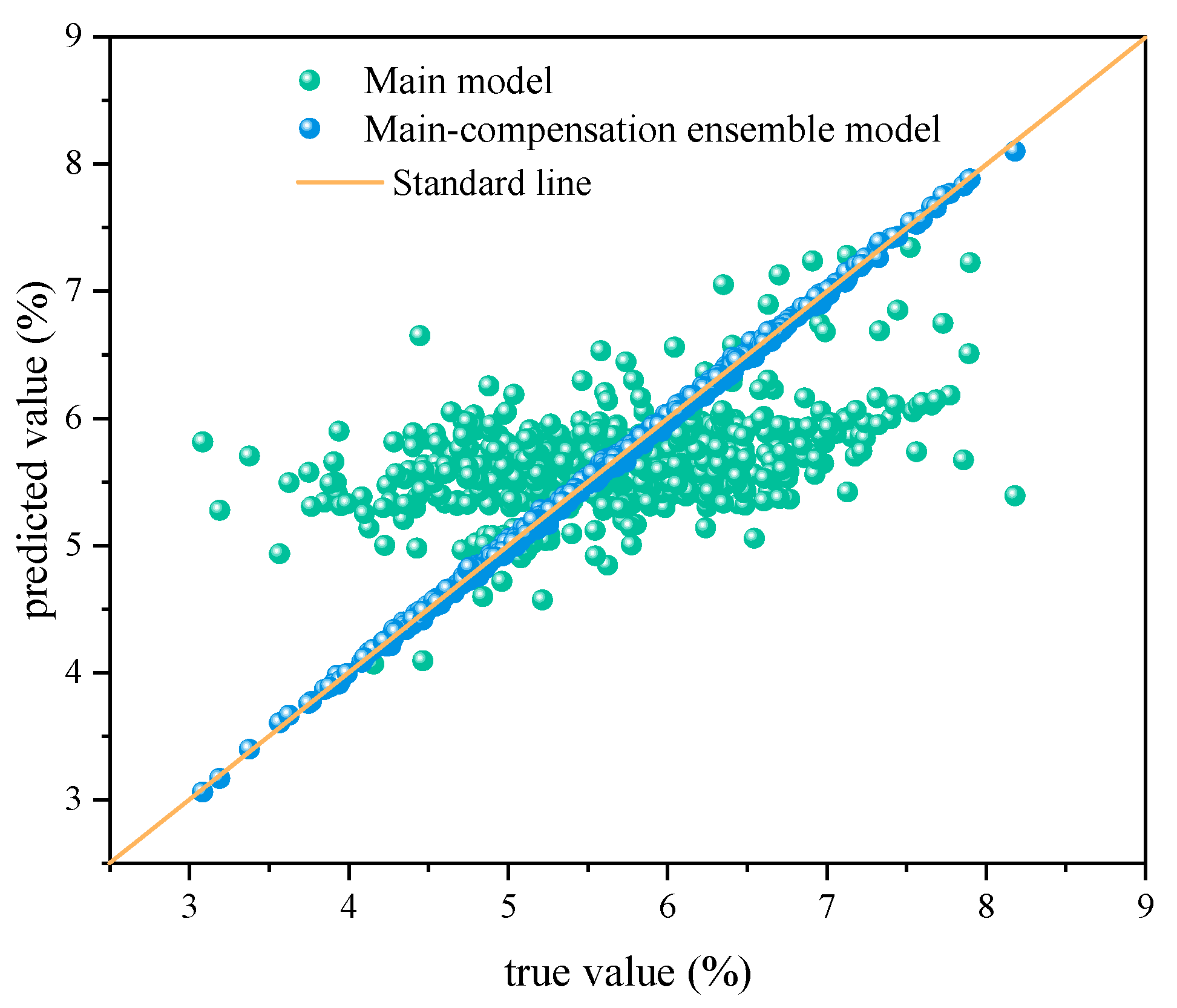
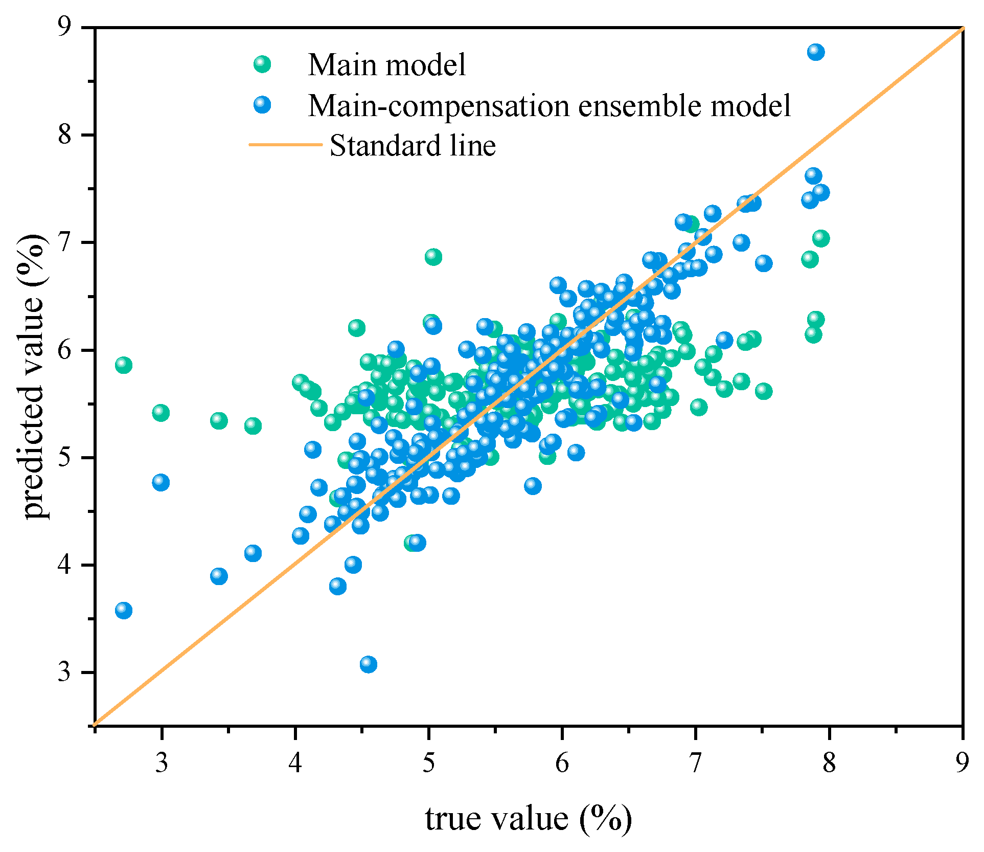
3.2.2. Main–Compensation Ensemble Modeling Results

The weights of all trees used to construct the main model are shown in Figure 8.
The curve of the objective function in the BO search process is shown in Figure 9.
Figure 9 shows that the value of the objective function is in the range of −0.50794 to −0.79876 in the BO process.
The scatter plots between the true values and the predicted values of the training set and testing set are shown in Figure 10 and Figure 11.
Statistical results of performance evaluation indices for the training set and testing set of main model and main–compensation ensemble model are shown in Table 1.
For the scatter plot between the true values and the predicted values, the closer the points are to the standard line ( y ^ = y ), the better the fitting effect is. According to Figure 10 and Figure 11, when only the main model is used, the predicted value is far from the standard line. After using the main–compensation ensemble model, for the training set, the predicted values can basically fit the standard line; for the testing set, the fitting effect has also been greatly improved. At the same time, according to Table 1, after adding the compensation model, the training set and the testing set are tested. The results show a decrease in RMSE and MAE, along with an increase in R2. It shows that the performance of the model has been greatly improved. In addition, the main model utilizes EnTSFRT algorithm, which provides good interpretability. In the process of constructing the tree, the number of rules and characteristics of fuzzy reasoning are clear and can be visualized. After training, the structure and internal weights of the TSFRT sub-model are also effectively visualized.

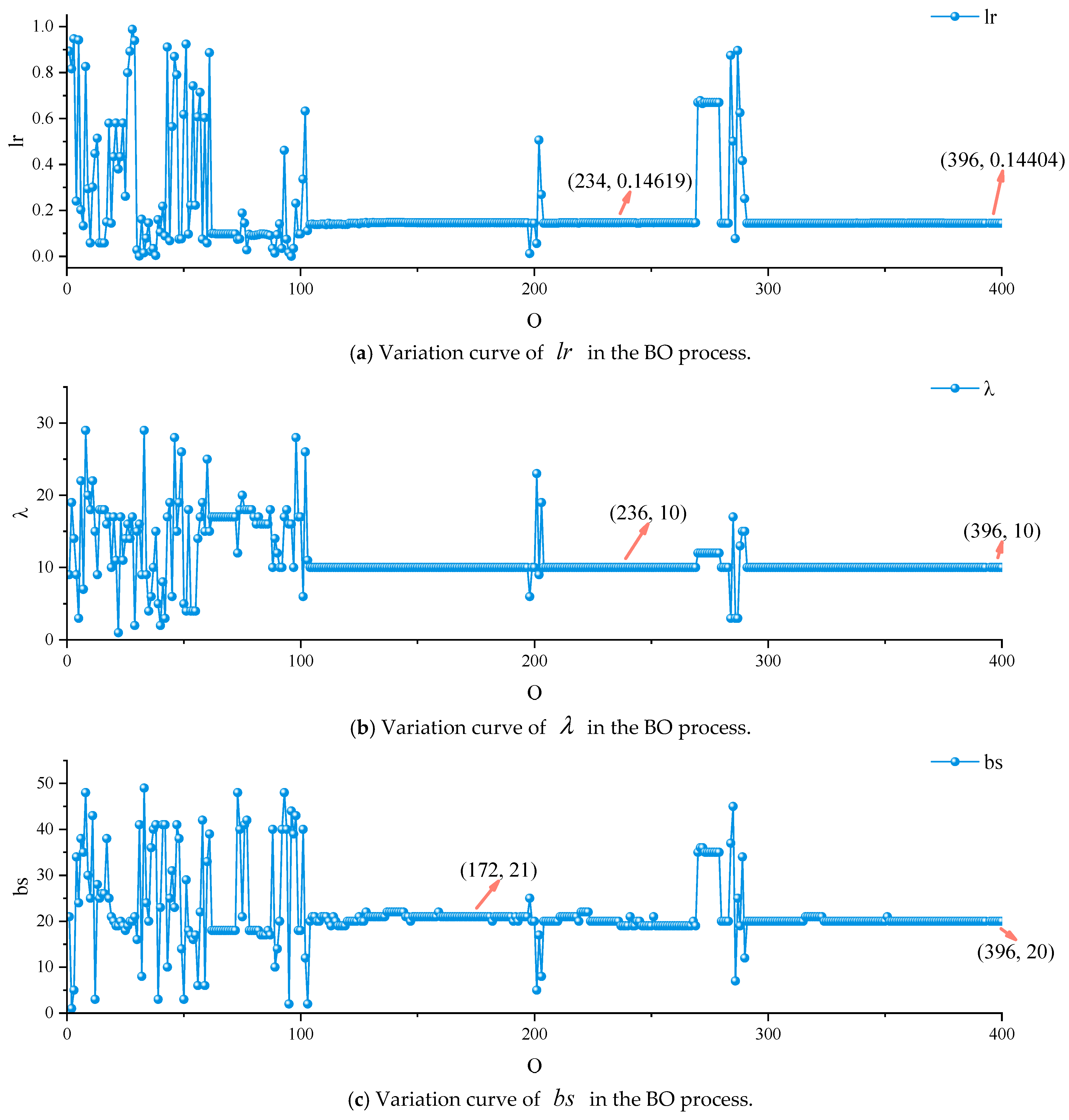
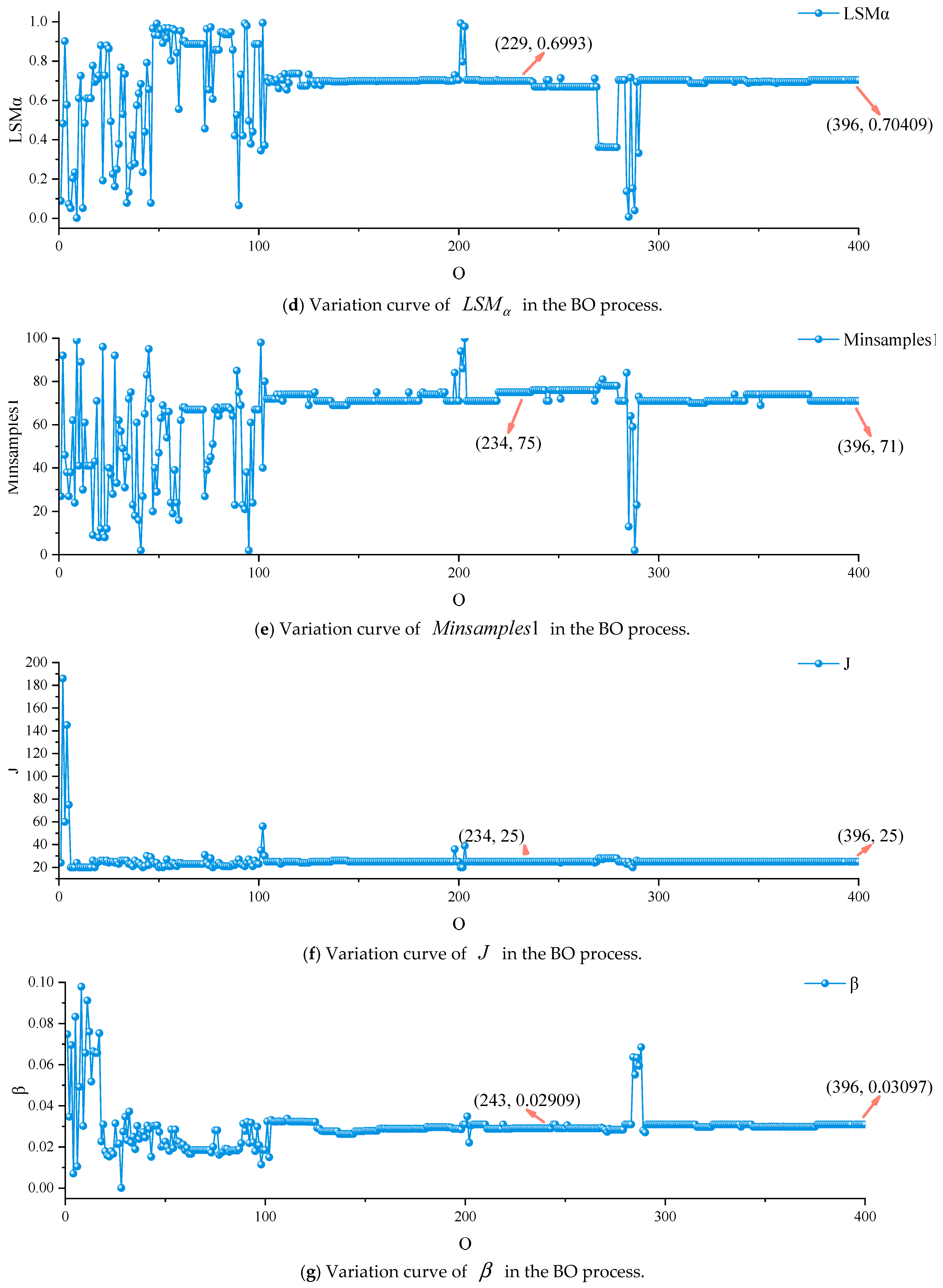
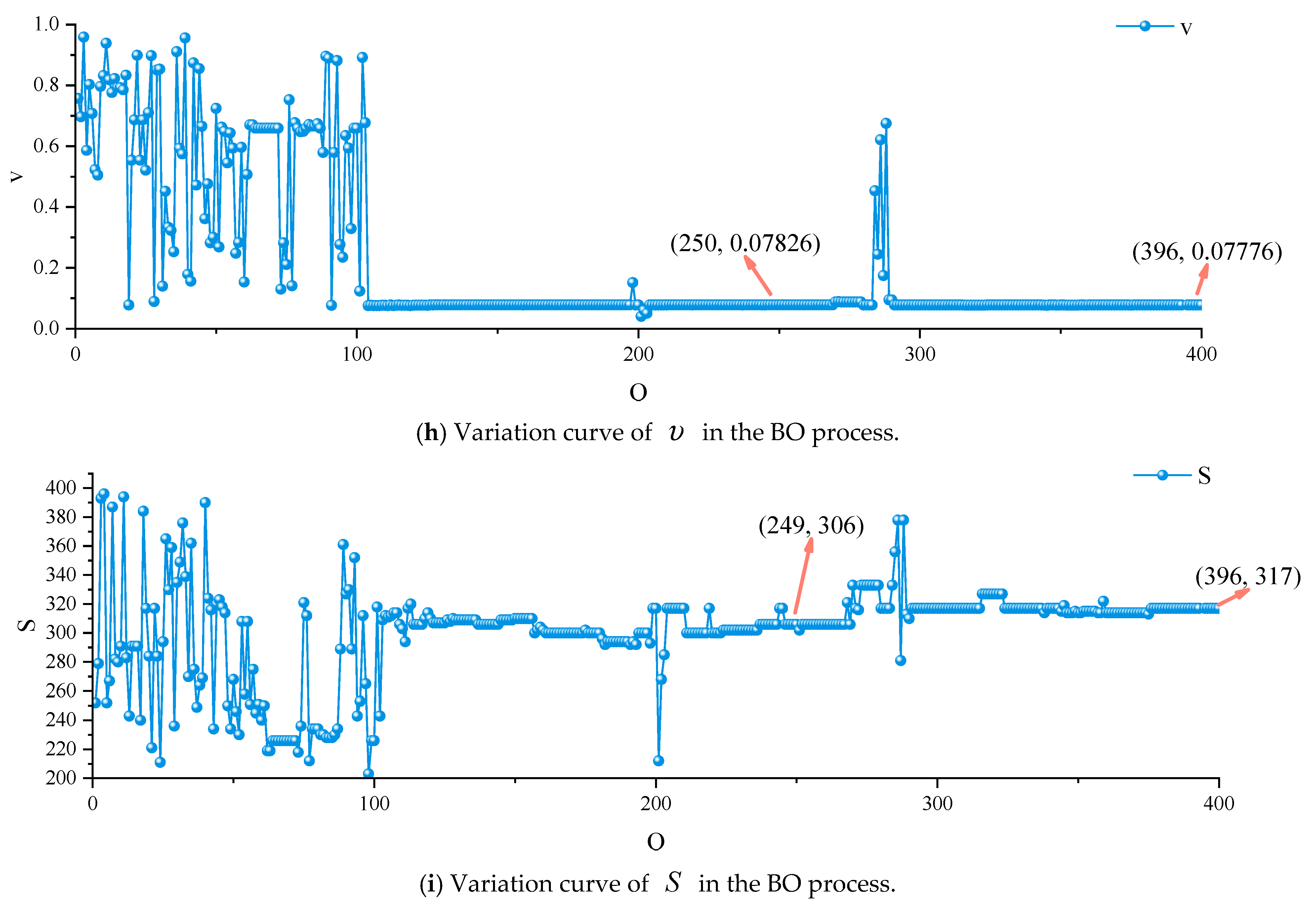
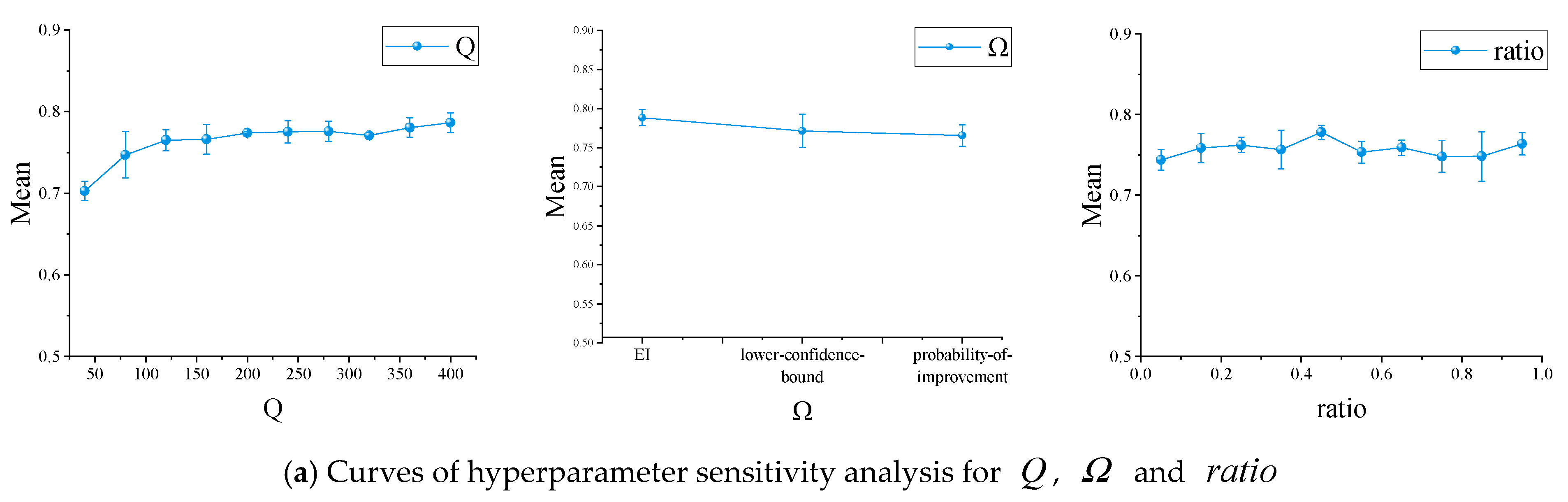
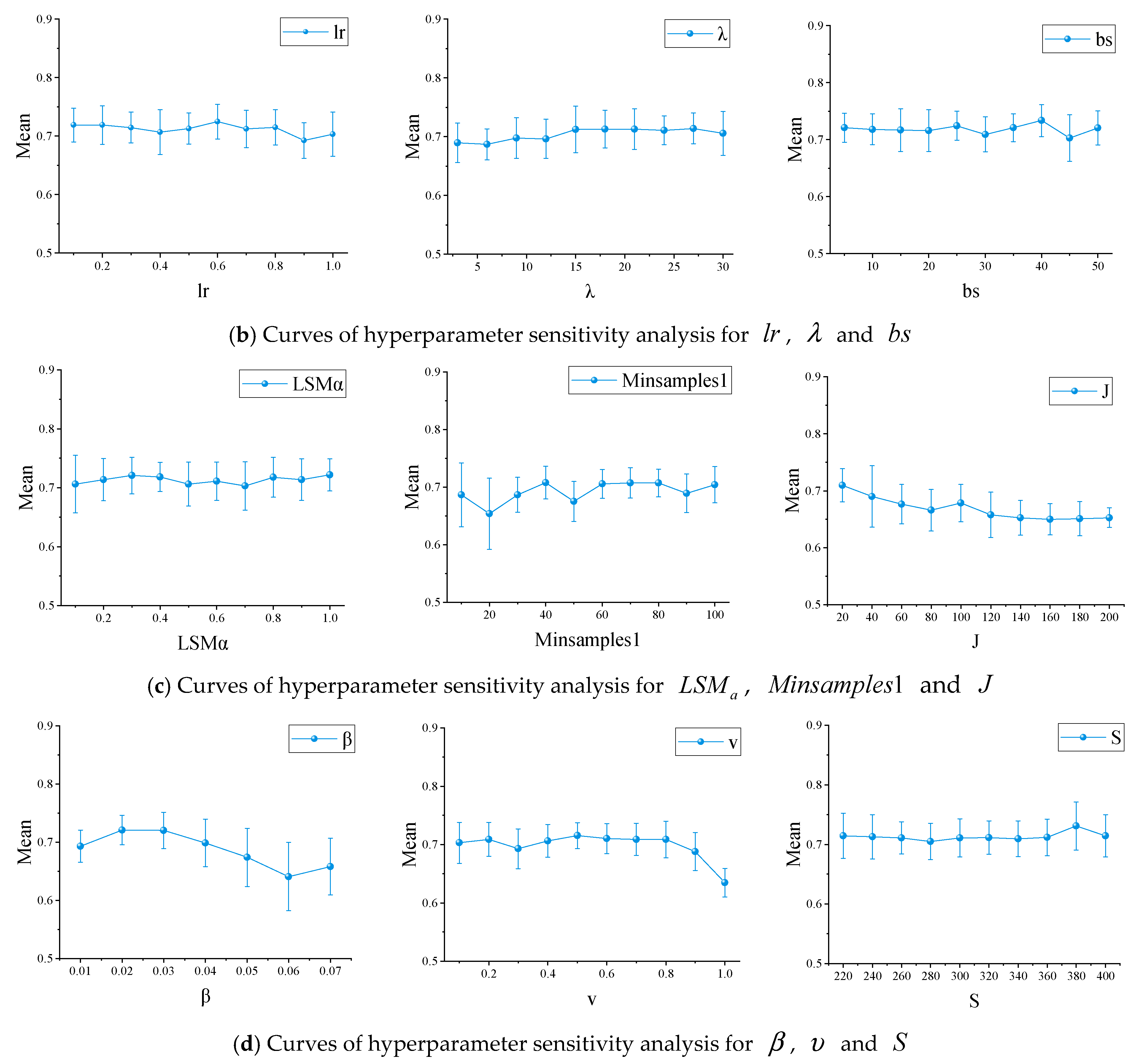
3.2.3. Hyperparameter Variation Results Based on BO

The variation curves of the nine hyperparameters in the BO process are shown in Figure 12.
Figure 12 shows the changes in hyperparameters of the main–compensation ensemble model during the BO search process. The specific detailed analysis is as follows.
(1) Figure 12a shows the change curve of l r , which is the learning rate of the main model. When the range of Q is 0 to 130, the change in l r is dramatic. When Q is in the ranges of 130 to 197 and 204 to 269, the value of l r remains stable at around 0.15. After that, the value of l r exhibits significant fluctuations. And when Q exceeds 291, the value of l r eventually stabilizes at around 0.14. So, choosing the appropriate Q is necessary.
(2) Figure 12b shows the change curve of λ , which is the initial value of the intermediate variable in the recursive calculation process of the main model. With the increase in Q , its change trend is similar to that of l r . Its value eventually stabilizes around 10.
(3) Figure 12c shows the change curve of b s , which is the number of batches of the main model training. When Q is in the ranges of 104 to 197 and 204 to 269, the value of b s fluctuates within a small range. When Q is in the range of 269 to 291, the value of b s changes dramatically. After that, when Q exceeds 291, the fluctuations in b s become smaller, eventually converging to 20.
(4) Figure 12d shows the change curve of L S M a , which is the regularization coefficient of the main model. With the increase in b s , its change trend is similar to that of l r . Its value eventually stabilizes at about 0.70.
(5) Figure 12e shows the change curve of M i n S a m p l e s 1 , which is the minimum number of leaf node samples of the main model. With the increase in Q , the value of M i n S a m p l e s 1 first changes dramatically. When Q is in the ranges of 104 to 197 and 204 to 283, the value of M i n S a m p l e s 1 fluctuates within a small range. Subsequently, it undergoes significant changes until Q exceeds 290, after which M i n S a m p l e s 1 resumes fluctuating within a small range and eventually converges to 71.
(6) Figure 12f shows the change curves of J , which is the number of decision trees of the main model. When Q is in the range of 0 to 6, the value of J changes drastically. When Q is greater than 6, the overall range of J fluctuates within a small margin and eventually converges to 25.
(7) Figure 12g shows the change curve of β , which is the learning rate of the compensation model. When Q is less than 104, the value of β exhibits a wide range of fluctuations. When Q is in the range of 104 to 283, β fluctuates around 0.03. Subsequently, it undergoes significant changes until Q exceeds 291, after which β fluctuates within a small range and eventually converges to 0.03.
(8) Figure 12h shows the change curve of υ , which is the regularization coefficient of the compensation model. With the increase in Q , its change trend is similar to that of β . The value of υ eventually stabilizes around 0.08.
(9) Figure 12i shows the change curve of S , which is the iteration times of the compensation model. When Q is in the ranges of 104 to 198 and 211 to 267, S fluctuates within a small range. Subsequently, it undergoes significant fluctuations until Q exceeds 291, after which S resumes fluctuating within a small range and eventually converges to 317.
Therefore, there is mutual coupling between these hyperparameters, and their behavior during the BO search process becomes even more complex. The analysis above, which examines the variation in a single hyperparameter with increasing iteration count, does not effectively capture this interactive effect. Additionally, determining the optimal number of optimization iterations remains an open problem that requires further investigation.

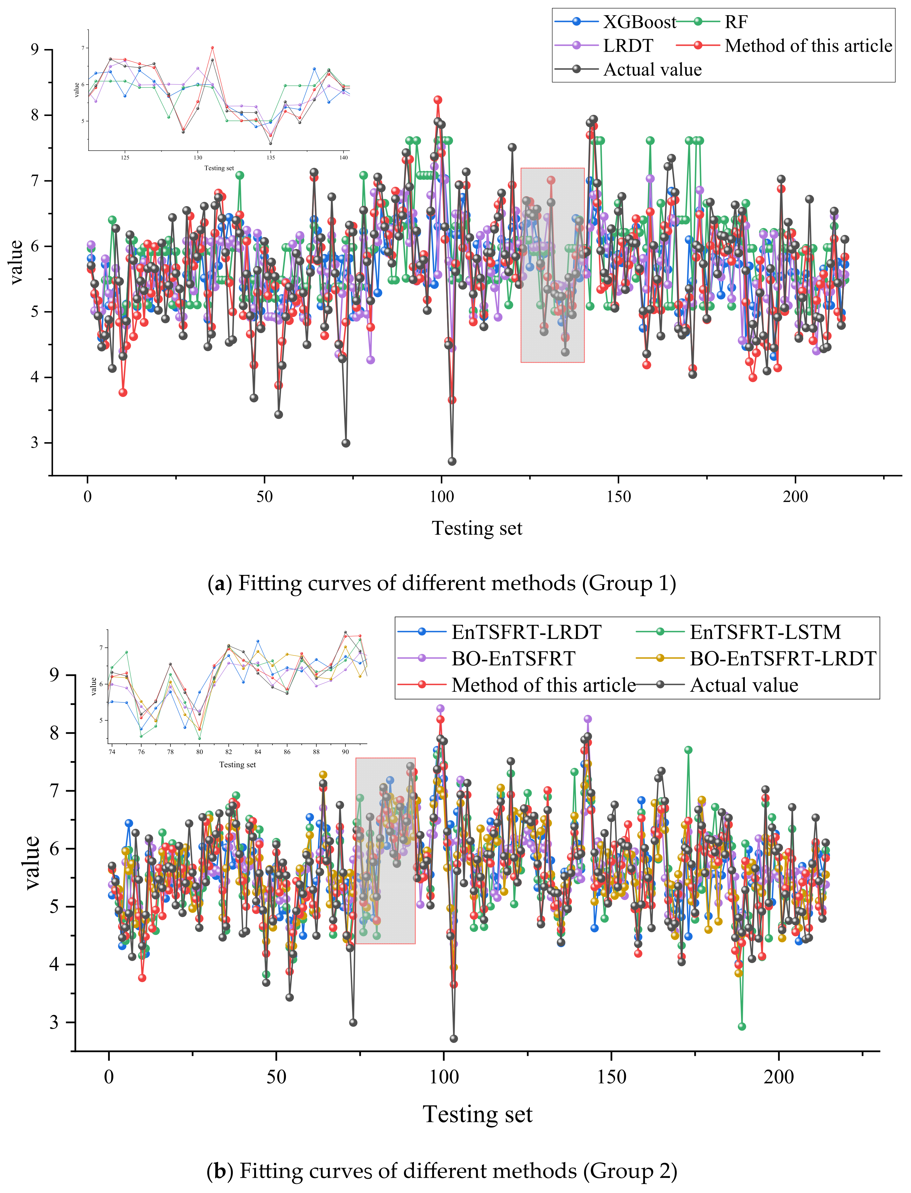
3.3. Method Comparison

To further illustrate the effectiveness, the proposed method is compared with tree-based methods such as eXtreme gradient boosting (XGBoost), random forest (RF), linear regression decision tree (LRDT), EnTSFRT-LRDT, and BO-EnTSFRT. This article employs grid search for selecting the hyperparameters of the comparison methods. The basic principle involves exploring all possible combinations of hyperparameters, then evaluating the model performance for each set of parameters using methods such as cross-validation, and ultimately selecting the optimal parameters. The hyperparameters of each model are set as follows. In the XGBoost model, the minimum number of samples is set to 10, the number of features is 5, the number of decision trees is 40, the learning rate is 0.3, and the regularization coefficient is 0.5. In the RF model, the minimum number of samples is set to 50, and the number of features is 5. In the LRDT model, the minimum number of samples is set to 20, and the regularization coefficient is 0.4. In the EnTSFRT-LRDT model, l r = 0.1 , λ = 10 , b s = 18 , L S M a = 0.3 , M i n S a m p l e s 1 = 30 , J = 160 , M i n S a m p l e s 2 = 35 , and β = 0.3 . In the EnTSFRT-LSTM model, l r = 0.1 , λ = 15 , b s = 18 , L S M a = 0.3 , M i n S a m p l e s 1 = 55 , J = 80 , β = 0.05 , υ = 0.3 , S = 320 . In the BO-EnTSFRT model, l r = 0.8554 , λ = 18 , b s = 41 , L S M a = 0.919 , M i n S a m p l e s 1 = 45 , and J = 200 . In the BO-EnTSFRT-LRDT model, l r = 0.024 , λ = 6 , b s = 48 , L S M a = 0.6123 , M i n S a m p l e s 1 = 77 , J = 184 , M i n S a m p l e s 2 = 22 , and β = 0.1346 . It should be noted that M i n S a m p l e s 2 is the minimum number of samples of the LRDT model.
Based on the above models, the modeling and testing experiments are repeated 20 times. Table 2 shows the statistical results of the performance evaluation indices of different methods with 20 repetitions. One of the fitting curves and the overall statistical results are shown in Figure 13.
Figure 13 shows that the proposed method achieves the best fitting performance compared to the other methods. In Table 2, XGBoost has the best performance among the three tree-based main model methods. The proposed BO-EnTSFRT-LSTM model has the lowest average RMSE and MAE for both the training set (2.6610 × 10⁻², 2.0684 × 10⁻²) and the testing set (4.3991 × 10⁻¹, 3.1771 × 10⁻¹). At the same time, the proposed method has the highest R2 on the training set (9.9896 × 10⁻¹) and the testing set (7.5649 × 10⁻¹ ± 2.4804 × 10⁻⁴). By comparing the method proposed in this article with EnTSFRT-LSTM and BO-EnTSFRT, the important role of the BO algorithm and the LSTM-based compensation model is illustrated, respectively. In addition, the comparison between the proposed method and the BO-EnTSFRT-LRDT further illustrates the superiority of the LSTM algorithm. The proposed BO-EnTSFRT-LSTM method utilizes EnTSFRT to handle uncertainty in industrial modeling data, uses LSTM to fit error data, and applies BO to optimize hyperparameters that are prone to overfitting, resulting in optimal modeling performance. Comparisons with other methods demonstrate the superiority of the proposed method.
Through the above comparative experiments and causal analysis, it is indicated that the proposed method based on BO-EnTSFRT-LSTM has the best performance.

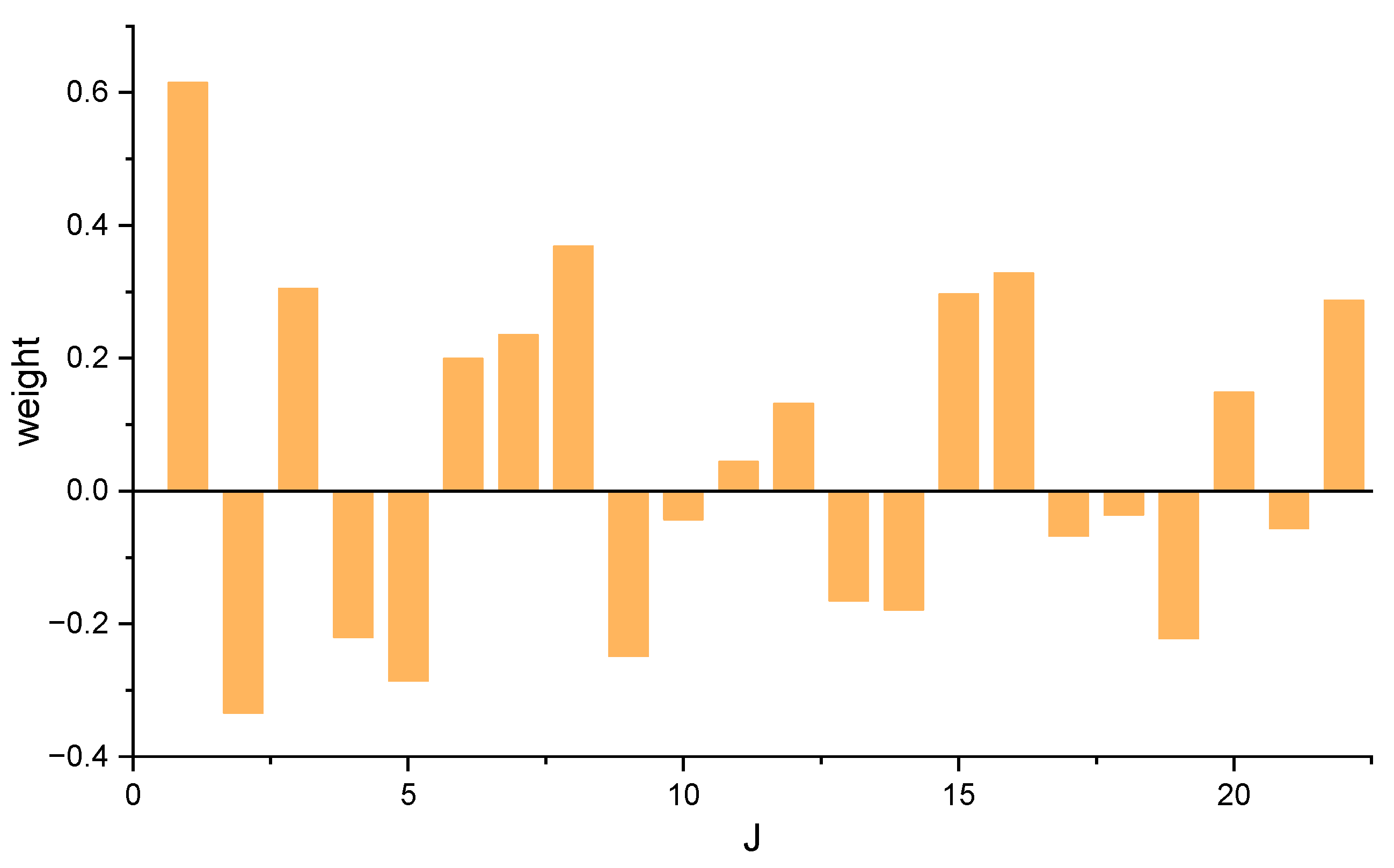
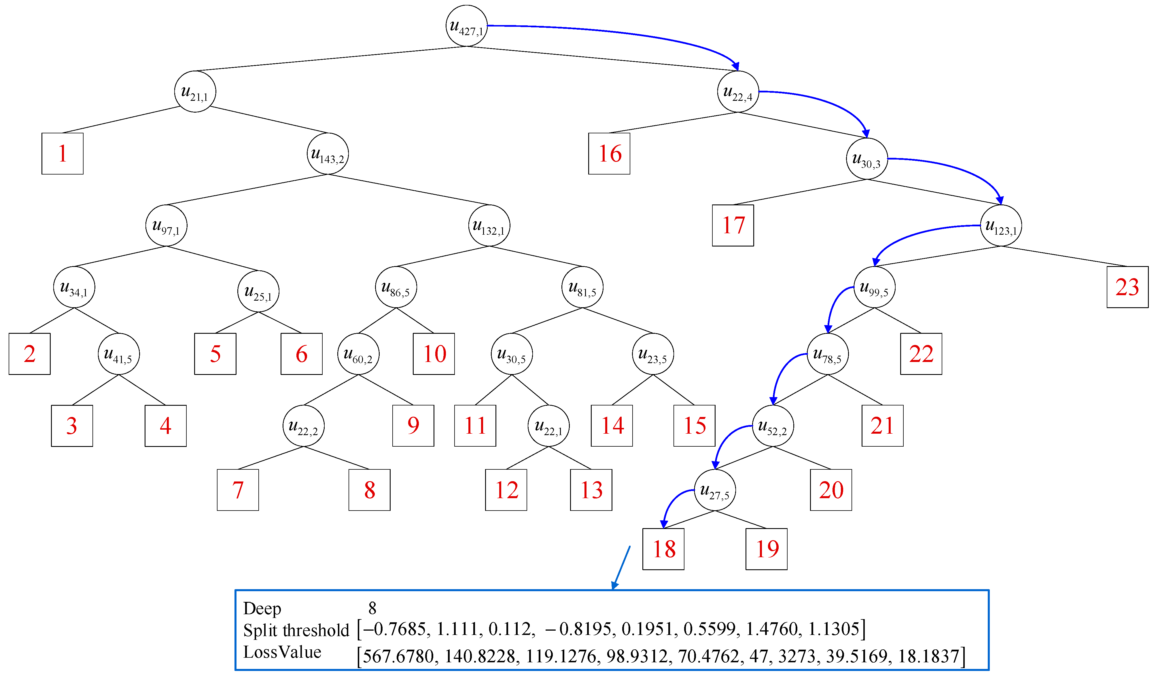
3.4. Interpretability Analysis

To illustrate the interpretability of the EnTSFRT model, the generation process of the first tree is described as an example. The generation process is shown in Figure 14.
In Figure 14, the red numbers indicate the indices of the leaf nodes. To better illustrate its interpretability, we analyze the path indicated by the blue arrow in Figure 14.
For the original training set, when selecting the first feature of the 427th sample as the split point, i.e., (427, 1), the loss value is minimized at 567.6780. The split threshold at this point is −0.7685. Samples with the first feature greater than this threshold are assigned to the right subset, while the rest are assigned to the left subset. This process corresponds to Equations (6)–(10). The above process is repeated until the number of samples in all leaf nodes is less than the minimum sample size, and no further splitting is performed. During this process, the selected split points are (427, 1), (22, 4), (30, 3), (123, 1), (99, 5), (78, 5), (52, 2), and (27, 5), with the corresponding split thresholds being −0.7685, 1.1110, 0.1120, −0.8195, 0.1951, 0.5599, 1.4760, and 1.1305, and the corresponding loss values being 567.6780, 140.8228, 119.1276, 98.9312, 70.4762, 47.3273, 39.5169, and 18.1837.
The above process is repeated until the tree is fully generated. Based on Equations (11) and (12), the inputs to the fuzzy reasoning layer can be obtained.
According to Equation (15), the membership function can be calculated as follows:
0.278349915944106 0.974011271399689 0.993706466740484 0.978108098565900 0.973056705111963 0.999468131326339 0.825395356069636 0.751123667701550 0.998444623241835 0.976409615360689 0.966675618127725 1.16099938349223 e 270 0.987714527031402 0.165187018507589 0.990313811263087 0.199359948173210 0.954610652912701 0.918292332286325 0.981902393519507 0.696142421345977 0.742304366809322 0.838927685814161 0.920768272181872 0.996908111439030 0.999854194791565
Using the minimum membership method for rule matching, the minimum value of each column is selected as the activation intensity of the rule, as shown in Equation (16). The final activation intensities are obtained as follows:
0.199359948173210 1.16099938349223 e 270 0.751123667701550 0.165187018507589 0.696142421345977
The weights for the consequent part are as follows:
2.12345169618872 0.467836590298729 0.387025848195383 0.409185879800525 0.179931644262229
corresponding to Equation (21).
Then, based on Equation (18), the predicted output value can be obtained.
Therefore, the interpretability of TSFRT is mainly reflected in the following aspects:
(1) The model has good visualization results. As shown in Figure 14, non-leaf nodes are represented by circles, and leaf nodes are represented by squares, with a model depth of 8. Additionally, the split coordinates, sample count, and feature count are all visualized.
(2) The TS fuzzy reasoning process can be interpreted from three perspectives. First, the TSFRT model uses a binary tree structure, providing a unique computational path. Second, the depth of the TSFRT model in this article is relatively shallow, which enhances its interpretability. Third, the consequent layer of the TS fuzzy reasoning system at the leaf nodes is a linear function, making the input–output relationship straightforward and contributing to the model’s higher interpretability.

3.5. Hyperparameter Discussion

In the study, the single-factor sensitivity analysis of the hyperparameters is carried out. A total of 10 sets of experiments are set for each hyperparameter (except for Ω ). The selection of step size should consider the sensitivity of hyperparameters and the limitations of computing resources. In this study, the experiment is conducted with a fixed step size according to the setting interval of the hyperparameters based on author’s debug experience and PC hardware performance. The interval setting and step size are shown in Table 3.
Table 3 shows the initial value and the step size for different hyperparameters as follows: (1) the initial value of Q is 40, and the step size is 40; (2) Ω takes EI, lower-confidence-bound, and probability-of-improvement, respectively; (3) the initial value of r a t i o is 0.05, and the step size is 0.1; (4) the initial value of l r is 0.1, and the step size is 0.1; (5) the initial value of λ is 3, and the step size is 3; (6) the initial value of b s is 5, and the step size is 5; (7) the initial value of L S M a is set to 0.1, and the step size is 0.1; (8) the initial value of M i n S a m p l e s 1 is 10, and the step size is 10; (9) the initial value of J is 20, and the step size is 20; (10) the initial value of β is 0.01, and the step size is 0.01; (11) the initial value of υ is 0.05, and the step size is 0.1; and (12) the initial value of S is 220, and the step size is 20.
The experiment uses R2 as the evaluation metric, and the results, obtained through 20 repeated trials, are shown in Figure 15.
Figure 15 indicates that different hyperparameters of the constructed BO-EnTSFRT-LSTM model have varying effects. A detailed analysis is provided below.
(1) Figure 15a shows the effects of Q , Ω , and r a t i o on the performance of the BO-EnTSFRT-LSTM model. When Q is in the intervals [40, 280] and [320, 400], the mean value of R2 shows an increasing trend, and when Q is larger, the standard deviation fluctuates less. It indicates that a larger Q is more likely to achieve a model with better performance, but in practical applications, the computational resource consumption needs to be considered. When Ω is the EI function, the mean value of R2 is the largest (0.7885), and the standard deviation is the smallest (0.01025). It indicates that the model performance is optimal at this point. When the ratio is 0.45, the mean value of R2 reaches its maximum. When the r a t i o is 0.45, the mean value of R2 reaches its maximum (0.7777). When Q is in the range [0.45, 0.65], the mean and standard deviation of R2 fluctuate less, indicating that a moderate ratio value is more likely to yield a high-performance model.
(2) Figure 15b shows the effects of l r , λ , and b s on the performance of the BO-EnTSFRT-LSTM model. When l r is less than 0.5, the mean value of R2 fluctuates less. When l r = 0.6 , the mean value of R2 reaches its maximum (0.7246). It shows that it is easier to meet the requirements when l r is small. If the l r is too large, it may cause the model to skip over the optimal solution, which makes the model unable to achieve the best performance. When λ is in the interval [15, 27], the mean value of R2 fluctuates less. It shows that it is easier to meet the conditions when the value of λ is larger. As the b s increases and falls within the range of 5 to 20, the mean value of R2 fluctuates less. When b s = 40 , the mean value of R2 reaches its maximum (0.7333).
(3) Figure 15c shows the effects of L S M a , M i n S a m p l e s 1 , and J on the performance of the BO-EnTSFRT-LSTM model. With the increase in L S M a , the mean value of R2 increases rapidly. When L S M a is less than 0.3, the mean value of R2 shows an increasing trend, while the standard deviation exhibits a decreasing trend. When L S M a is 1, the mean value of R2 is the highest (0.7218). When M i n S a m p l e s 1 is greater than 40, the fluctuations in its mean and standard deviation are smaller. It shows that a larger M i n S a m p l e s 1 makes it easier to obtain a higher-performance model. When J is in the range of 20 to 80 and 100 to 160, the mean of R2 decreases rapidly. And when J is 20, the mean value of R2 is the highest (0.7096). It shows that it is easier to obtain a high-performance model when J is small.
(4) Figure 15d shows the effects of β , υ , and S on the performance of the BO-EnTSFRT-LSTM model. When β is 0.02, the mean value of R2 reaches its maximum (0.7207), and the standard deviation is the smallest (0.02537). As β increases beyond 0.07, the learning rate is too large, resulting in gradient explosion. Therefore, in order to avoid gradient explosion, a smaller β should be selected. When υ is less than 0.8, the fluctuation in the mean of R2 remains relatively small. When υ is 0.5, the mean of R2 is the highest (0.7152), and the corresponding standard deviation is smallest (0.02220). And when υ exceeds 0.8, the mean of R2 decreases rapidly. When S is in the range of 220 to 340, the mean of R2 fluctuates within a small range. The mean of R2 increases rapidly when S is in the range of 340 to 380. And when S is 380, the mean of R2 reaches its peak (0.7306).
It is important to note that the sensitivity analysis conducted here is based on individual hyperparameters. In reality, these hyperparameters are interdependent, which is one of the reasons why BO is used for hyperparameter selection in this study.

3.6. Comprehensive Analysis

The proposed method in this article has some limitations in each module as follows.
(1) When constructing the main model base on the EnTSFRT algorithm, which consists of multiple decision trees and fuzzy rulers, the training process consumes significant computing resources. Further research is needed on how to perform structural reduction and ruler optimization on the construction of the main model based on the pruning algorithm. Moreover, how to further enhance the ability of the EnTSFRT algorithm to represent uncertainties in the modeling data also needs to be explored.
(2) When constructing the compensation model based on LSTM, issues such as gradient disappearance or gradient explosion may occur. At the same time, the structure of LSTM is complex and the training process is slow. Therefore, future research can focus on improving the structure of the LSTM model by exploring lightweight algorithms.
(3) During the process of hyperparameter optimization using BO, there is a risk of falling into local optima, especially when dealing with high-dimensional, non-convex functions that exhibit unknown smoothness and noise. Since the BO algorithm often faces challenges in addressing this issue, enhancing its ability and adaptability to such problems is a critical task that requires attention. Additionally, further consideration is needed regarding the application of BO to non-Gaussian distributed data, which may be present in actual industrial processes.
In summary, the experimental results presented here were obtained for flue gas oxygen content under a single operating condition of the actual MSWI process. Addressing a wider range of operating conditions with multiple CVs remains an open problem in academic and industrial fields. One potential solution is to develop separate models for different operating conditions. Given the complexity of the actual MSWI process, multiple CVs must be considered simultaneously. In this study, only one CV (flue gas oxygen content) was considered. Future research could focus on the modeling and control of multiple CVs under multiple operating conditions.

4. Conclusions

Stable control of flue gas oxygen content during the MSWI process is crucial for enhancing incineration efficiency and reducing pollutant emissions. To address the challenge of a lack of high-precision and interpretable models for flue gas oxygen content in the context of intelligent control algorithms, this article proposes a flue gas oxygen content model based on the BO-EnTSFRT-LRDT algorithm. The main contributions are as follows: (1) A hybrid model that integrates both a main model and a compensation model, combining a non-neural ensemble algorithm with a neural deep learning algorithm, is proposed. (2) A strategy is introduced that uses BO to optimize the hyperparameters of the main–compensation ensemble model. (3) For the first time, an interpretable and high-precision controlled object model for flue gas oxygen content is developed. Experimental results demonstrate that the proposed method outperforms other existing methods, confirming its feasibility and effectiveness. The results show that the RMSE and MAE are reduced by 48.2% and 53.1%, respectively, while the R2 increases by 140.8% compared to the modeling method that relies solely on the main model.
In addition, there are some limitations in this study. Due to the use of TSFRT and LSTM, the model demands high computational resources during the training phase. Moreover, improving the capability and adaptability of the BO algorithm remains an open issue. Further research is also needed to explore how to apply BO to industrial data with a non-Gaussian distribution. In future research, the limitations outlined above need to be addressed. Additionally, the number of hidden layers and neurons in each layer is to be reduced to simplify the LSTM model. Similarly, the number and depth of trees in the TSFRT model are to be optimized to minimize the model size. More importantly, a control algorithm needs to be designed and implemented based on this foundation to ensure the efficient and stable operation of the MSWI process.

Author Contributions

Conceptualization, J.T.; Methodology, W.Y. and J.T.; Resources, T.W.; Data curation, T.W.; Writing—original draft, W.Y.; Writing—review & editing, J.T. and H.T. All authors have read and agreed to the published version of the manuscript.

Funding

This research received no external funding.

Institutional Review Board Statement

Not applicable.

Informed Consent Statement

Not applicable.

Data Availability Statement

The data presented in this study are available on request from the corresponding author.

Conflicts of Interest

The authors declare no conflict of interest.

Appendix A

Table A1. Detailed description of each element in Figure 1.
OrderStageElementsDescriptions
1Solid waste fermentationCrab bucketIt is primarily used to grab MSW and transport it from the waste reservoir to the feeding inlet of the incinerator.
2Solid waste reservoirIt is used for storing and pre-processing MSW that is awaiting incineration.
3Slag poolIt is used for collecting and processing the slag generated after incineration.
4Solid waste combustionHopperIt is a device used for the temporary storage and transportation of MSW.
5Auxiliary burnerIt is a key device used to provide additional heat.
6FeederIt is a device used to transport MSW from the hopper to the incinerator.
7Drying grateIt is used for the drying and pre-processing of MSW.
8Combustion grateIt is a key device used for the combustion of MSW.
9Burner grateIt is a device used for the burnout of MSW and the handling of slag.
10SSCIt is used to process the slag generated after incineration, achieving the dual goals of resource recovery and environmental protection by separating metals, cooling the slag, and reducing environmental pollution.
11Primary air fanIt is a key device used to supply the primary air required for combustion.
12Secondary air fanIt is a key device used to supply secondary air.
13Air preheatingThrough certain equipment or systems, the air temperature is raised to a predetermined level.
14Denitration systemA system that removes nitrogen oxides (NOx) from flue gases through chemical or physical methods.
15Steam power generationTurbogeneratorTransforming the heat energy generated during the incineration process into electricity.
16Waste heat exchangeSteamThe high-temperature, high-pressure gas generated by heating water through a boiler is mainly used for converting and utilizing the thermal energy from waste heat.
17SuperheaterThe already evaporated saturated steam is further heated to raise its temperature, converting it into superheated steam.
18EvaporatorWaste heat or other heat sources are utilized to heat the liquid to its boiling point and evaporate it into steam.
19EconomizerBy recovering and utilizing the waste heat from flue gases, this preheats the cold water entering the boiler or other equipment.
20Water supplyProvides the necessary cold water for the waste heat exchange system, which, after waste heat exchange, can absorb heat and circulate within the system.
21Flue gas G1It is the flue gas emitted from the outlet of the waste heat boiler, which contains high concentrations of various pollutants and requires cleaning treatment.
22Hammering equipmentThrough mechanical vibration or tapping, it helps remove dirt, deposits, or other substances that may accumulate on the surface of the heat exchanger and obstruct heat transfer.
23Ash conveyorCollects and transports the ash generated during the combustion process from the combustion equipment to the designated processing or storage area.
24Flue gas cleaningReclaimed waterIt is treated wastewater.
25ReactorRemoves or transforms harmful substances in flue gas through chemical or physical processes.
26Bag filterUsed to remove solid particles from flue gas, effectively capturing dust, particulate matter, and other pollutants in the flue gas through physical filtration.
27MixerEvenly mixes different gases or liquid components to achieve a more effective cleaning treatment.
28Fly ash tankUsed to collect and store the fly ash removed from the flue gas.
29Flue gas G2It is cleaned flue gas that is discharged into the chimney through an induced draft fan.
30Induced draft fanDischarges flue gas, maintains system pressure, and promotes airflow.
31Flue gas emissionDioxinsIt is generated by the reaction of chlorine and aromatic hydrocarbons under high-temperature conditions, usually as a byproduct of the combustion process.
32COIt is generated by the reaction of carbon and oxygen under incomplete combustion conditions, and is a colorless, odorless, and tasteless gas.
33SO2It is a common pollutant generated by the reaction of sulfur and oxygen, and is typically released during the combustion of sulfur-containing fuels.
34CO2It is one of the main greenhouse gases produced in the combustion process.
35NOxIt consists of thermal NOx, which is formed by the oxidation of nitrogen (N2) in the air at high temperatures during combustion, and fuel NOx, which is generated from the combustion of nitrogen-containing organic matter in waste. It is one of the major pollutants in incineration flue gas.
36HClIt is one of the major acidic pollutants in the flue gas, primarily originating from the combustion of chlorine-containing substances in the waste.
37Particulate matterIt is one of the important pollutants in the flue gas, primarily composed of incompletely combusted solid particles, fly ash, heavy metal oxides, and salt particles formed by the reaction of acidic gases with alkaline substances.
38Flue gas G3It is the flue gas emitted into the atmosphere through chimneys, and the concentration of pollutants it contains must meet the requirements of the national environmental protection department.
39ChimneyIt is the final channel for flue gas emissions from the incineration plant, primarily used to discharge the cleaned flue gas into the atmosphere.
Table A2. Abbreviations and their meanings.
OrderEnglish AbbreviationEnglish Full Name
1.MSWMunicipal solid waste
2.MSWIMSW incineration
3.AIArtificial intelligence
4.CVControlled variable
5.DXNDioxin
6.SO2Sulfur dioxide
7.NNNeural network
8.LSTMLong short-term memory
9.ILSTMImproved LSTM
10.TSTakagi–Sugeno
11.TSFNNTS fuzzy neural network
12.MIMOMultiple-input multiple-output
13.EnTSFRTTS fuzzy regression tree
14.SCRSelective catalytic reduction
15.GBDTGradient boosting decision tree
16.BOBayesian optimization
17.MVManipulated variable
18.PCCPearson correlation coefficient
19.MSEMean square error
20.RNNRecurrent neural network
21.EIExpected improvement
22.R2R-square
23.UBUpper boundary
24.LBLower boundary
25.GPRGaussian process regression
26.MLEMaximum likelihood estimation
27.RMSERoot mean square error
28.MAEMean absolute error
29.eXtreme gradient boostingXGBoost
30.Random forestRF
31.Linear regression decision treeLRDT
Table A3. Symbols and their meanings.
OrderSymbolMeaning
1. u Manipulated variables
2. y True value of flue gas oxygen content
3. y ^ main Output value of flue gas oxygen content of the main model
4. e ^ main Error value of the main model
5. e ^ comp Output value of the compensation model
6. e ^ mix Error value of the compensation model
7. y ^ Output value of BO-EnTSFRT-LSTM model
8. l r Learning rate
9. b s Number of batches
10. λ Initial value of intermediate variable in the recursive calculation process
11. L S M α Regularization coefficient of the main model
12. M i n S a m p l e s 1 Minimum number of samples of the main model
13. J Number of sub-models that constitute the EnTSFRT model
14. β Learning rate of the compensation model
15. υ Regularization coefficient of the compensation model
16. S Maximum number of iterations of the compensation model
17. D Input of EnTSFRT
18. n Index of the sample
19. N Total number of input samples
20. M Dimension of the input feature
21. m Index of the input feature
22. u n n th input sample in D
23. y n True value of the n th sample in D
24. j Index of the training subset
25. U j Input   variable   matrix   of   the   j th training subset
26. D j j th training subset obtained by performing random sampling with the Bootstrap method on D
27. D Left j , 1 Left subset obtained by splitting the first non-leaf node
28. D Right j , 1 Right subset obtained by splitting the first non-leaf node
29. y j True value vector of flue gas oxygen content
30. M j Number   of   nodes   in   the   j th TSFRT sub-model
31. M nonleaf j Number of non-leaf nodes in the j th TSFRT sub-model
32. m nonleaf j Index of the non-leaf nodes in the j th TSFRT sub-model
33. M leaf j Number of leaf nodes in the j th TSFRT sub-model
34. m leaf j Index of the leaf nodes in the j th TSFRT sub-model
35. Φ Minimum   loss   value   when   the   split   point   is   n , m
36. D Left j , m nonleaf j Left   subset   of   the   m nonleaf j th   non - leaf   node   in   the   j th TSFRT sub-model
37. D Right j , m nonleaf j Right   subset   of   the   m nonleaf j th   non - leaf   node   in   the   j th TSFRT sub-model
38. f MSE m nonleaf j MSE value of the left subset D Left j , m nonleaf j (or right subset D Right j , m nonleaf j )
39. y Left j , m nonleaf j True   vectors   of   the   left   subset   D Left j , m nonleaf j
40. y Right j , m nonleaf j True   vectors   of   the   right   subset   D Right j , m nonleaf j
41. μ c s j , m nonleaf j Clear   membership   function   of   input   at   the   m nonleaf j th non-leaf node
42. ϑ Left j , m nonleaf j Average   of   the   target   values   of   the   left   subset   D Left j , m nonleaf j
43. ϑ Right j , m nonleaf j Average   of   the   target   values   of   the   left   subset   D Right j , m nonleaf j
44. N j , m nonleaf j Number of samples in the D Left j , m nonleaf j (or D Right j , m nonleaf j )
45. ϕ m nonleaf j j Segmentation   threshold   at   the   m nonleaf j th non-leaf node
46. C cs j , m leaf j Clear   set   at   the   m leaf j th leaf node
47. ϕ 1 j First   element   in   the   clear   set   C cs j , m leaf j
48. C cs _ 1 j , m leaf j Initial   clear   set   at   the   m leaf j th leaf node
49. N Left j , m nonleaf j Number   of   samples   in   the   D Left j , m nonleaf j
50. N Right j , m nonleaf j Number   of   samples   in   the   D Right j , m nonleaf j
51. D j , m leaf j Sample   of   the   m leaf j th leaf node
52. D fuzzy j , m leaf j Fuzzy reasoning layer corresponding to the m leaf j th leaf node
53. u n j , m leaf j j , m leaf j n j , m leaf j th input vector of the m leaf j th fuzzy reasoning layer
54. u n j , m leaf j , m nonleaf j j , m leaf j m nonleaf j th feature of n j , m leaf j th input vector of the m leaf j th fuzzy reasoning layer
55. N j , m leaf j Number of samples in the m leaf j th leaf node
56. K Total number of fuzzy rules
57. k Index of the fuzzy rule
58. μ A n j , m leaf j , m nonleaf j k j Membership degree of u n j , m leaf j , m nonleaf j j , m leaf j belonging to A n j , m leaf j , m nonleaf j j , k
59. y j , k Output   of   the   k th fuzzy rule
60. g j , k Nonlinear function between u n j , m leaf j j , m leaf j and y j , k
61. ω j , k Consequent   part   of   the   k th rule
62. ω m nonleaf j j , k Weight   of   the   input   variable   u n j , m leaf j , m nonleaf j j , m leaf j
63. δ n j , m leaf j , m nonleaf j j , k Center   of   the   membership   function   μ A n j , m leaf j , m nonleaf j j , k j
64. σ n j , m leaf j , m nonleaf j j , k Width   of   membership   function   μ A n j , m leaf j , m nonleaf j j , k j
65. α j , k Activation   intensity   of   the   k th fuzzy rule
66. m nonleaf j = 1 M nonleaf j Cartesian product
67. α ¯ j , k Normalized   value   of   α j , k
68. Φ back Loss   function   value   when   m nonleaf j non-leaf nodes are split
69. ω 0 j , k Weight of the initial time
70. Φ m nonleaf j back m nonleaf j th value in Φ back
71. H n j , m leaf j j Intermediate variable in the recursive process
72. H 0 j Initial   value   of   H n j , m leaf j j
73. λ A large positive value
74. I Unit matrix
75. y ^ n j Predicted   value   of   u n j   by   the   j th sub-model
76. F N samples
77. W LSM T n Weight matrix of TSFRT sub-models when EnTSFRT model is contrusted
78. t Current moment (iteration time)
79. h Hidden state
80. c Cell state
81. c ˜ Candidate cell state
82. ζ Sigmoid function
83. ψ Tanh function
84. f Value of the forget gate
85. i Value of the input gate
86. o Value of the output gate
87. Element-by-element multiplication
88. D E Input of the compensation model
89. W Weight matrix
90. b Bias matrix
91. W out Output weight matrix
92. J t Loss function in the training process of LSTM
93. x 1 , , x 9 Hyperparameters set for BO
94. Q Optimization number of BO iterations
95. Ω EI sampling function
96. r a t i o Exploration ratio
97. D Number of sample features
98. q Number of iterations of the q th optimization
99. p Number of data set samples at the current time
100. P init Number of initial inputs for the BO algorithm
101. Γ Objective function value corresponding to the observation sample
102. x op Optimal   point   that   minimizes   the   objective   function   Γ x op
103. ξ 0 Mean function
104. Σ 0 Covariance matrix
105. σ 2 Variance of noise
106. Σ 0 ( x a , x b ) Kernel function between a th and b th sample points
107. x a o The   o th   dimensional   feature   of   the   a th sample
108. σ Γ Kernel amplitude of kernel function
109. η o Length   ratio   of   the   o th dimension of the sample
110. Σ 0 Training testing set covariance
111. ξ p Posterior mean value
112. σ p 2 Posterior variance
113. x New samples obtained by updating the data set in BO process
114. M i n S a m p l e s 2 Minimum number of samples of LRDT model

References

  1. Gómez-Sanabria, A.; Kiesewetter, G.; Klimont, Z.; Schoepp, W.; Haberl, H. Potential for future reductions of global GHG and air pollutants from circular waste management systems. Nat. Commun. 2022, 13, 106. [Google Scholar] [PubMed]
  2. Ali, K.; Kausar, N.; Amir, M. Impact of pollution prevention strategies on environment sustainability: Role of environmental management accounting and environmental proactivity. Environ. Sci. Pollut. Res. 2023, 30, 88891–88904. [Google Scholar]
  3. Song, Y.; Xian, X.; Zhang, C.; Zhu, F.; Yu, B.; Liu, J. Residual municipal solid waste to energy under carbon neutrality: Challenges and perspectives for China. Resour. Conserv. Recycl. 2023, 198, 107177. [Google Scholar]
  4. Tang, J.; Xia, H.; Yu, W.; Qiao, J. Research status and prospect of intelligent optimization control of municipal solid waste incineration process. Acta Autom. Sin. 2023, 49, 2019–2059. [Google Scholar]
  5. Chen, A.; Chen, J.; Cui, J.; Fan, C.; Han, W. Research on risks and countermeasures of “cities besieged by waste” in China-an empirical analysis based on DIIS. Bull. Chin. Acad. Sci. 2019, 34, 797–806. [Google Scholar]
  6. Efforts to Promote the Realization of Carbon Peak Carbon Neutral Target. Available online: https://www.ndrc.gov.cn/wsdwhfz/202111/t20211111_1303691.html (accessed on 15 January 2025).
  7. Walser, T.; Limbach, L.K.; Brogioli, R.; Erismann, E.; Flamigni, L.; Hattendorf, B.; Juchli, M.; Krumeich, F.; Ludwig, C.; Prikopsky, K.; et al. Persistence of engineered nanoparticles in a municipal solid-waste incineration plant. Nat. Nanotechnol. 2012, 7, 520–524. [Google Scholar] [CrossRef]
  8. Zhang, Y.; Wang, L.; Chen, L.; Ma, B.; Zhang, Y.; Ni, W.; Tsang, D. Treatment of municipal solid waste incineration fly ash: State-of-the-art technologies and future perspectives. J. Hazard. Mater. 2021, 411, 125132. [Google Scholar]
  9. Lu, J.-W.; Zhang, S.; Hai, J.; Lei, M. Status and perspectives of municipal solid waste incineration in China: A comparison with developed regions. Waste Manag. 2017, 69, 170–186. [Google Scholar]
  10. Zhang, M.; Wei, J.; Li, H.; Chen, Y.; Liu, J. Comparing and optimizing municipal solid waste (MSW) management focused on air pollution reduction from MSW incineration in China. Sci. Total. Environ. 2024, 907, 167952. [Google Scholar]
  11. Chen, Z.; Wang, L.; Huang, Z.; Zhuang, P.; Shi, Y.; Evrendilek, F.; Huang, S.; He, Y.; Liu, J. Dynamic and optimal ash-to-gas responses of oxy-fuel and air combustions of soil remediation biomass. Renew. Energy 2024, 225, 120229. [Google Scholar]
  12. Zhao, P.; Gao, Y.; Sun, X. The impact of artificial intelligence on pollution emission intensity—evidence from China. Environ. Sci. Pollut. Res. 2023, 30, 91173–91188. [Google Scholar] [CrossRef]
  13. Ding, Y.; Zhao, J.; Liu, J.-W.; Zhou, J.; Cheng, L.; Zhao, J.; Shao, Z.; Iris, Ç.; Pan, B.; Li, X.; et al. A review of China’s municipal solid waste (MSW) and comparison with international regions: Management and technologies in treatment and resource utilization. J. Clean. Prod. 2021, 293, 126144. [Google Scholar] [CrossRef]
  14. Qiao, J.; Sun, J.; Meng, X. Event-triggered adaptive model predictive control of oxygen content for municipal solid waste incineration process. IEEE Trans. Autom. Sci. Eng. 2022, 21, 463–474. [Google Scholar] [CrossRef]
  15. Sun, J.; Meng, X.; Qiao, J. Data-driven predictive control of flue gas oxygen content in municipal solid waste incineration process. Control. Theory Appl. 2024, 41, 484–495. [Google Scholar]
  16. Huang, W.; Ding, H.; Qiao, J. Adaptive multi-objective competitive swarm optimization algorithm based on kinematic analysis for municipal solid waste incineration. Appl. Soft Comput. 2023, 149, 110925. [Google Scholar] [CrossRef]
  17. Sun, J.; Meng, X.; Qiao, J. Event-based data-driven adaptive model predictive control for nonlinear dynamic processes. IEEE Trans. Syst. Man Cybern. Syst. 2024, 54, 1982–1994. [Google Scholar] [CrossRef]
  18. Li, L.; Ding, S.; Yang, Y.; Peng, K.; Qiu, J. A fault detection approach for nonlinear systems based on data-driven realizations of fuzzy kernel representations. IEEE Trans. Fuzzy Syst. 2017, 26, 1800–1812. [Google Scholar] [CrossRef]
  19. Cho, S.; Kim, Y.; Kim, M.; Cho, H.; Moon, I.; Kim, J. Multi-objective optimization of an explosive waste incineration process considering nitrogen oxides emission and process cost by using artificial neural network surrogate models. Process. Saf. Environ. Prot. 2022, 162, 813–824. [Google Scholar] [CrossRef]
  20. Sildir, H.; Sarrafi, S.; Aydin, E. Optimal artificial neural network architecture design for modeling an industrial ethylene oxide plant. Comput. Chem. Eng. 2022, 163, 107850. [Google Scholar]
  21. Rahimieh, A.; Mehriar, M.; Zamir, S.M.; Nosrati, M. Fuzzy-decision tree modeling for H2S production management in an industrial-scale anaerobic digestion process. Biochem. Eng. J. 2024, 208, 109380. [Google Scholar] [CrossRef]
  22. Samek, W.; Montavon, G.; Lapuschkin, S.; Anders, C.J.; Muller, K.-R. Explaining deep neural networks and beyond: A review of methods and applications. Proc. IEEE 2021, 109, 247–278. [Google Scholar]
  23. Xia, H.; Tang, J.; Yu, W.; Cui, C.; Qiao, J. Takagi–Sugeno Fuzzy Regression Trees With Application to Complex Industrial Modeling. IEEE Trans. Fuzzy Syst. 2023, 31, 2210–2224. [Google Scholar]
  24. Ma, Y.; Zhou, Y.; Peng, J.; Chen, R.; Dai, H.; Hao, M.; Hu, G.; Xie, Y. Prediction of flue gas oxygen content of power plant with stacked target-enhanced autoencoder and attention-based LSTM. Measurement 2024, 235, 115036. [Google Scholar] [CrossRef]
  25. Lin, C.; Lee, C. Neural-network-based fuzzy logic control and decision system. IEEE Trans. Comput. 1991, 40, 1320–1336. [Google Scholar] [CrossRef]
  26. Wu, D.; Peng, R.; Mendel, J. Type-1 and interval type-2 fuzzy systems. IEEE Comput. Intell. Mag. 2023, 18, 81–83. [Google Scholar]
  27. Takalo-Mattila, J.; Heiskanen, M.; Kyllonen, V.; Maatta, L.; Bogdanoff, A. Explainable steel quality prediction system based on gradient boosting decision trees. IEEE Access 2022, 10, 68099–68110. [Google Scholar]
  28. Alrbai, M.; Al-Dahidi, S.; Alahmer, H.; Al-Ghussain, L.; Hayajneh, H.; Shboul, B.; Abusorra, M.; Alahmer, A. Utilizing waste heat in wastewater treatment plants for water desalination: Modeling and Multi-Objective optimization of a Multi-Effect desalination system using Decision Tree Regression and Pelican optimization algorithm. Therm. Sci. Eng. Prog. 2024, 54, 102784. [Google Scholar]
  29. Meng, T.; Zhang, W.; Huang, J.; Chen, Y.-H.; Chew, C.-M.; Yang, D.; Zhong, Z. Fuzzy reasoning based on truth-value progression: A control-theoretic design approach. Int. J. Fuzzy Syst. 2023, 25, 1559–1578. [Google Scholar] [CrossRef]
  30. Yang, T.; Ma, K.; Lv, Y.; Fang, F.; Chang, T. Hybrid dynamic model of SCR denitrification system for coal-fired power plant. In Proceedings of the 2019 IEEE 28th International Symposium on Industrial Electronics (ISIE), Vancouver, BC, Canada, 12–14 June 2019; pp. 106–111. [Google Scholar]
  31. Luo, A.; Liu, B. Temperature prediction of roller kiln based on mechanism and SSA-ELM data-driven integrated model. In Proceedings of the 2022 China Automation Congress (CAC), Xiamen, China, 25–27 November 2022; pp. 5598–5603. [Google Scholar]
  32. Dong, S.; Zhang, Y.; Liu, J.; Zhou, X.; Wang, X. Intelligent compensation prediction of leaching process based on GRU neural network. In Proceedings of the 2022 China Automation Congress (CAC), Xiamen, China, 25–27 November 2022; pp. 1663–1668. [Google Scholar]
  33. Li, B.; Tian, W.; Zhang, C.; Hua, F.; Cui, G.; Li, Y. Positioning error compensation of an industrial robot using neural networks and experimental study. Chin. J. Aeronaut. 2022, 35, 346–360. [Google Scholar]
  34. Friedman, J.H. Greedy function approximation: A gradient boosting machine. Ann. Stat. 2001, 29, 1189–1232. [Google Scholar] [CrossRef]
  35. Wang, W.; Deng, C.; Zhao, L. Research on the application of ellipsoid bound algorithm in hybrid modeling. Acta Autom. Sin. 2014, 40, 1875–1881. [Google Scholar]
  36. Zhang, R.; Tang, J.; Xia, H.; Chen, J.; Yu, W.; Qiao, J. Heterogeneous ensemble prediction model of CO emission concentration in municipal solid waste incineration process using virtual data and real data hybrid-driven. J. Clean. Prod. 2024, 445, 141313. [Google Scholar] [CrossRef]
  37. Ma, S.; Chen, Z.; Zhang, D.; Du, Y.; Zhang, X.; Liu, Q. Interpretable multi-task neural network modeling and particle swarm optimization of process parameters in laser welding. Knowl. Based Syst. 2024, 300, 112116. [Google Scholar]
  38. Deng, J.; Liu, G.; Wang, L.; Liu, G.; Wu, X. Intelligent optimization design of squeeze casting process parameters based on neural network and improved sparrow search algorithm. J. Ind. Inf. Integr. 2024, 39, 100600. [Google Scholar]
  39. Zhou, X.; Tan, J.; Yu, J.; Gu, X.; Jiang, T. Online robust parameter design using sequential support vector regression based Bayesian optimization. J. Math. Anal. Appl. 2024, 540, 128649. [Google Scholar]
Figure 1. MSWI process flow of typical grate furnace.
Sustainability 17 03048 g001
Figure 2. Structure of edge verification platform of MSWI power plant in Beijing.
Sustainability 17 03048 g002
Figure 3. PCC values between key MVs and flue gas oxygen content.
Sustainability 17 03048 g003
Figure 4. Modeling strategy. Where the blue square illustrates the concrete implementation process of the main-compensation ensemble model.
Sustainability 17 03048 g004
Figure 5. Structure of the main model based on EnTSFRT.
Sustainability 17 03048 g005
Figure 6. Structure of compensation model construction module based on LSTM.
Sustainability 17 03048 g006
Figure 7. Flow chart of BO-EnTSFRT-LSTM algorithm.
Sustainability 17 03048 g007
Figure 8. Weight distribution diagram of the tree that constitutes EnTSFRT-based main model.
Sustainability 17 03048 g008
Figure 9. Curve of the objective function in the BO search process.
Sustainability 17 03048 g009
Figure 10. Scatter plot between the true values and the predicted values of the training set.
Sustainability 17 03048 g010
Figure 11. Scatter plot between the true values and the predicted values of the testing set.
Sustainability 17 03048 g011
Figure 12. Variation curves of the nine hyperparameters in the BO process.
Sustainability 17 03048 g012aSustainability 17 03048 g012bSustainability 17 03048 g012c
Figure 13. Fitting curves of different methods on the testing set.
Sustainability 17 03048 g013
Figure 14. Curves of the generation process of the first tree. Where the squares represent leaf nodes, the numbers indicate the indices of the leaf nodes; and the blue arrows denote the generation path of one particular leaf node.
Sustainability 17 03048 g014
Figure 15. Curves of hyperparameter sensitivity analysis in terms of average value of 20 times.
Sustainability 17 03048 g015aSustainability 17 03048 g015b
Table 1. Statistical results of performance evaluation indices of the training set and testing set of main model and main–compensation ensemble model.
Data SetMethodRMSEMAER2
Training setMain model9.0385 × 10−17.2671 × 10−11.8305 × 10−1
Main–compensation ensemble model2.4573 × 10−21.9215 × 10−29.9912 × 10−1
Testing setMain model9.8680 × 10−17.8328 × 10−11.5956 × 10−1
Main–compensation ensemble model4.3497 × 10−13.1282 × 10−17.6216 × 10−1
Table 2. Statistical results of performance evaluation indices of different methods.
Data SetMethodRMSEMAER2
Training setXGBoost4.9222 × 10−1 ± 1.1614 × 10−63.6090 × 10−1 ± 2.4410 × 10−66.4713 × 10−1 ± 2.3640 × 10⁻⁶
RF8.6432 × 10−1 ± 1.1677 × 10−316.4993 × 10⁻¹ ± 1.2975 × 10⁻³²−8.8061 × 10⁻² ± 8.1092 × 10⁻³⁴
LRDT5.2664 × 10−1 ± 5.1899 × 10−324.0872 × 10⁻¹ ± 1.2975 × 10−325.9604 × 10⁻¹ ± 1.2975 × 10⁻³²
EnTSFRT-LRDT4.4932 × 10−1 ± 1.1640 × 10−43.5266 × 10−1 ± 8.4882 × 10−57.0088 × 10−1 ± 2.0645 × 10⁻⁴
EnTSFRT-LSTM4.5666 × 10−2 ± 4.1522 × 10−43.3945 × 10−2 ± 1.6713 × 10−49.9639 × 10−1 ± 1.7202 × 10⁻⁵
BO-EnTSFRT6.4563 × 10−1 ± 9.0752 × 10−55.1347 × 10−1 ± 6.8136 × 10−55.8308 × 10−1 ± 1.5481 × 10⁻⁴
BO-EnTSFRT-LRDT4.3465 × 10−1 ± 2.9193 × 10−323.4153 × 10⁻¹ ± 1.2975 × 10−327.2484 × 10⁻¹ ± 5.1899 × 10⁻³²
BO-EnTSFRT-LSTM2.6610 × 10−2 ± 5.8122 × 10−62.0684 × 10−2 ± 3.3649 × 10−69.9896 × 10−1 ± 3.8281 × 10⁻⁸
Testing setXGBoost7.4611 × 10−1 ± 5.7058 × 10−55.6974 × 10−1 ± 9.2326 × 10−63.0015 × 10−1 ± 1.9958 × 10⁻⁴
RF9.7815 × 10−1 ± 5.1899 × 10−327.4468 × 10⁻¹ ± 5.1899 × 10⁻³²−2.0272 × 10⁻¹ ± 1.2975 × 10⁻³²
LRDT7.6825 × 10−1 ± 0.00005.9607 × 10−1 ± 5.1899 × 10−322.5808 × 10⁻¹ ± 0.0000
EnTSFRT-LRDT7.3435 × 10−1 ± 3.5825 × 10−45.7583 × 10−1 ± 1.6158 × 10−42.4216 × 10−1 ± 1.4912 × 10⁻³
EnTSFRT-LSTM5.7702 × 10−1 ± 1.0583 × 10−34.2354 × 10−1 ± 6.3545 × 10−45.8020 × 10−1 ± 2.1789 × 10⁻³
BO-EnTSFRT8.5004 × 10−1 ± 5.7774 × 10−46.7746 × 10−1 ± 2.1606 × 10−43.1419 × 10−1 ± 1.4888 × 10⁻³
BO-EnTSFRT-LRDT6.4225 × 10−1 ± 1.2975 × 10−324.9011 × 10⁻¹ ± 5.1899 × 10−324.8149 × 10⁻¹ ± 2.9193 × 10⁻³²
BO-EnTSFRT-LSTM4.3991 × 10−1 ± 2.0766 × 10−43.1771 × 10−1 ± 1.1515 × 10−47.5649 × 10−1 ± 2.4804 × 10⁻⁴
Table 3. Interval setting of hyperparameters of the main–compensation ensemble model.
ModelHyperparameterRangeStep Size
BO Q [40, 400]40
Ω //
r a t i o [0.05, 1]0.1
Main Model l r [0.1, 1]0.1
λ [3, 30]3
b s [5, 50]5
L S M a [0.1, 1]0.1
M i n s a m p l e 1 [10, 100]10
J [20, 200]20
Compensation Model β [0.01, 0.1]0.01
υ [0.05, 1)0.05
S [200, 400]20
Disclaimer/Publisher’s Note: The statements, opinions and data contained in all publications are solely those of the individual author(s) and contributor(s) and not of MDPI and/or the editor(s). MDPI and/or the editor(s) disclaim responsibility for any injury to people or property resulting from any ideas, methods, instructions or products referred to in the content.

