
Remote Sensing and Geographic Information Systems Detection of Fossil Fuel Air Pollution Impact in Socially Fragile Areas


Abstract
1. Introduction
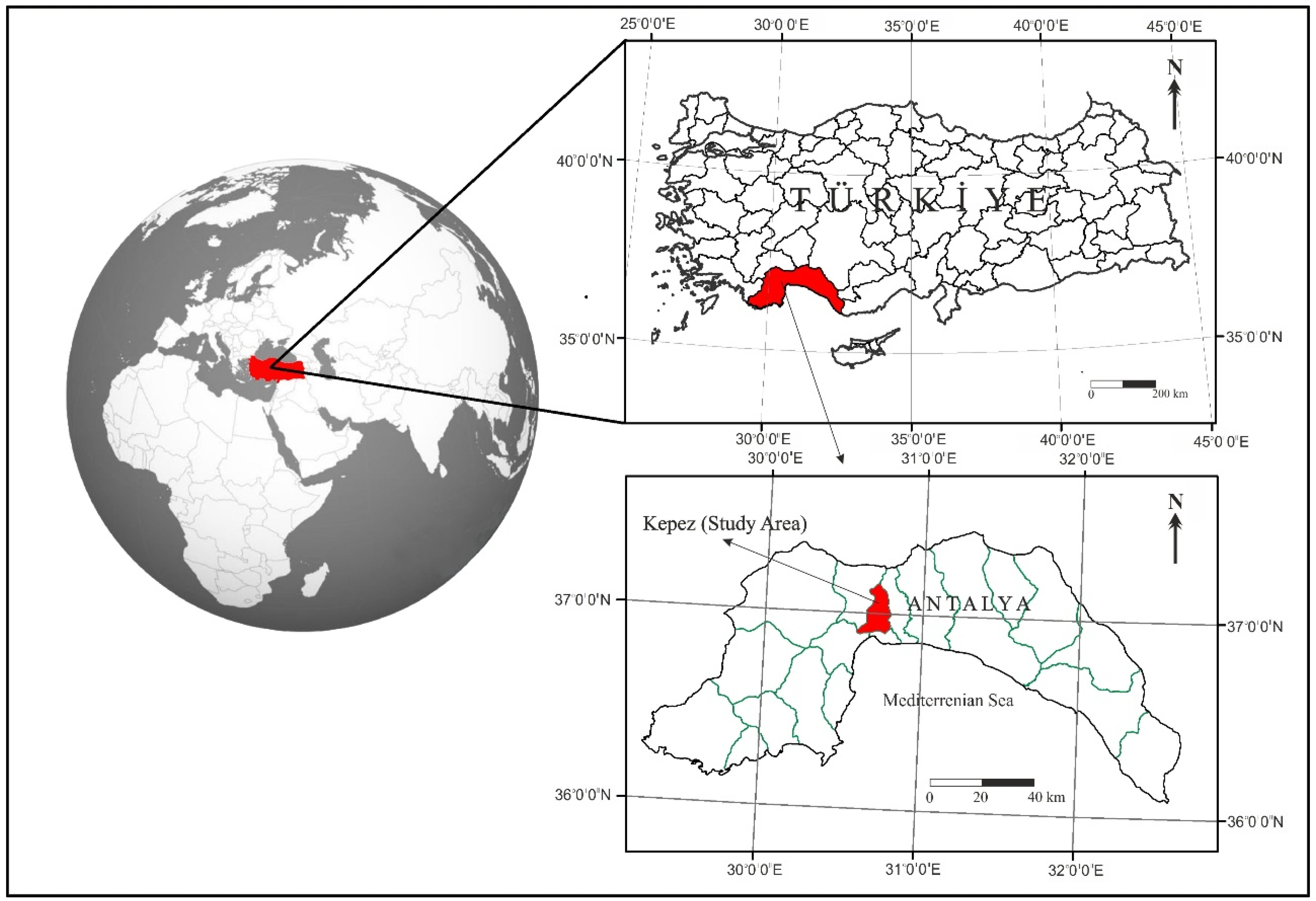
2. Study Area
3. Data Sets, Methods and Analysis
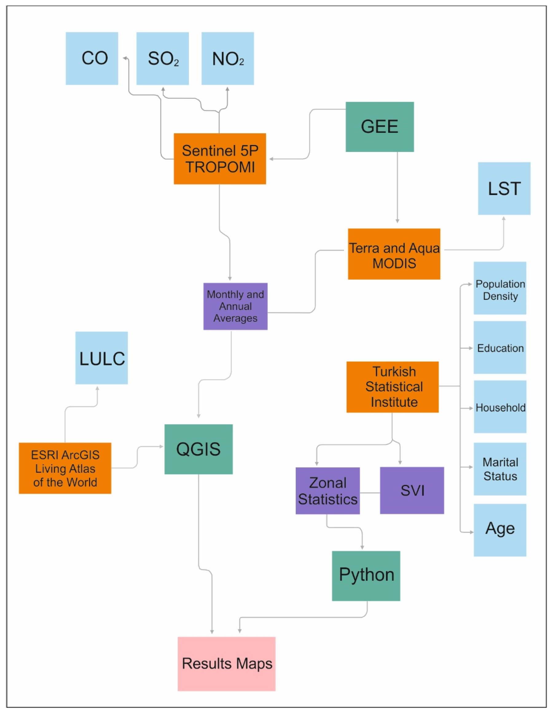
3.1. Data Sets and Preparation
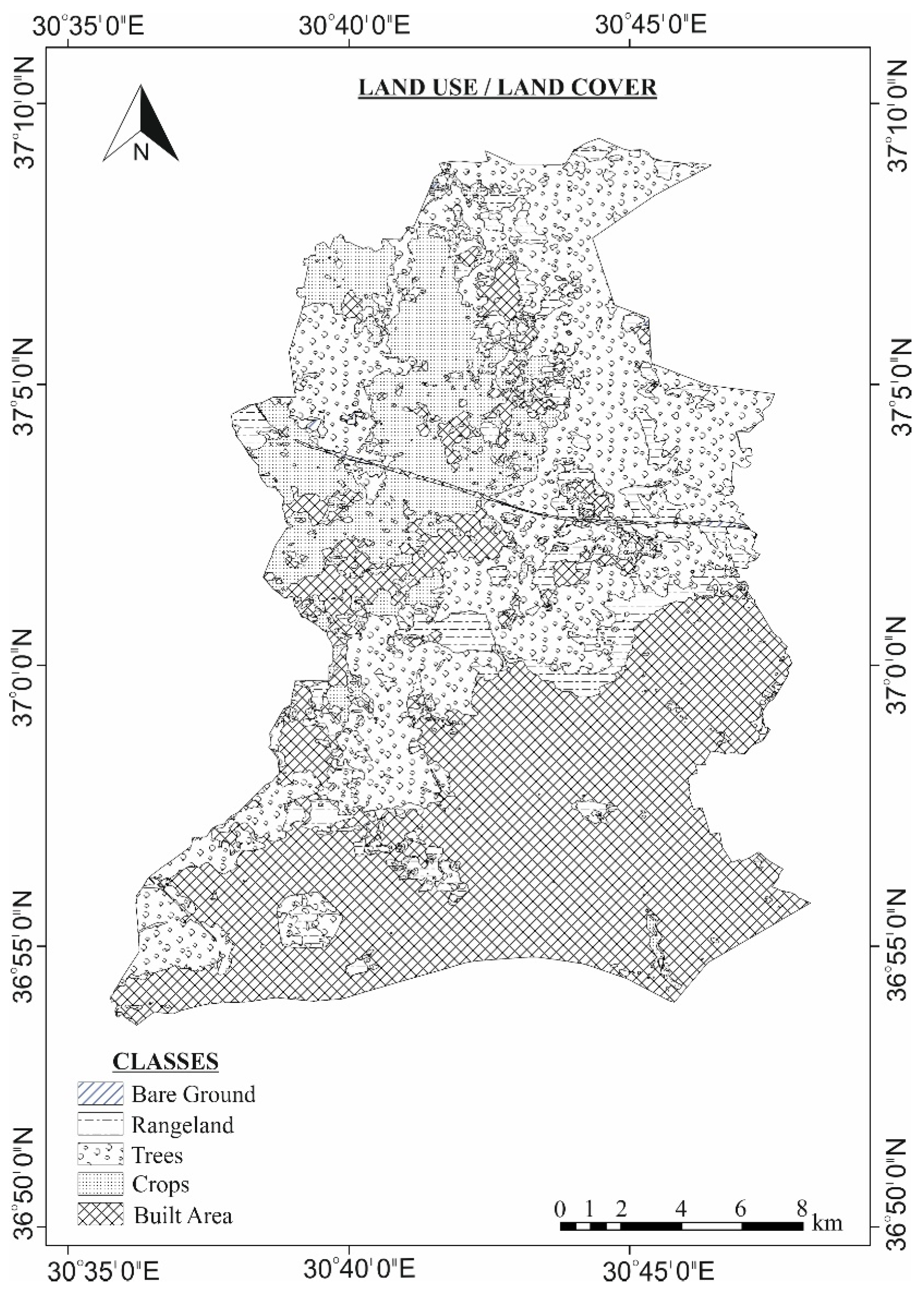
3.2. Land Use Land Cover (LULC)
3.3. Creating Air Pollutant Maps Using Open-Source Code
3.4. Air Pollution in the COVID-19 Pandemic in Kepez
3.5. Land Surface Temperature (LST)
3.6. Analyses with GIS Tool and Zonal Statistics
3.7. Statistical Analyses
4. Results and Discussion
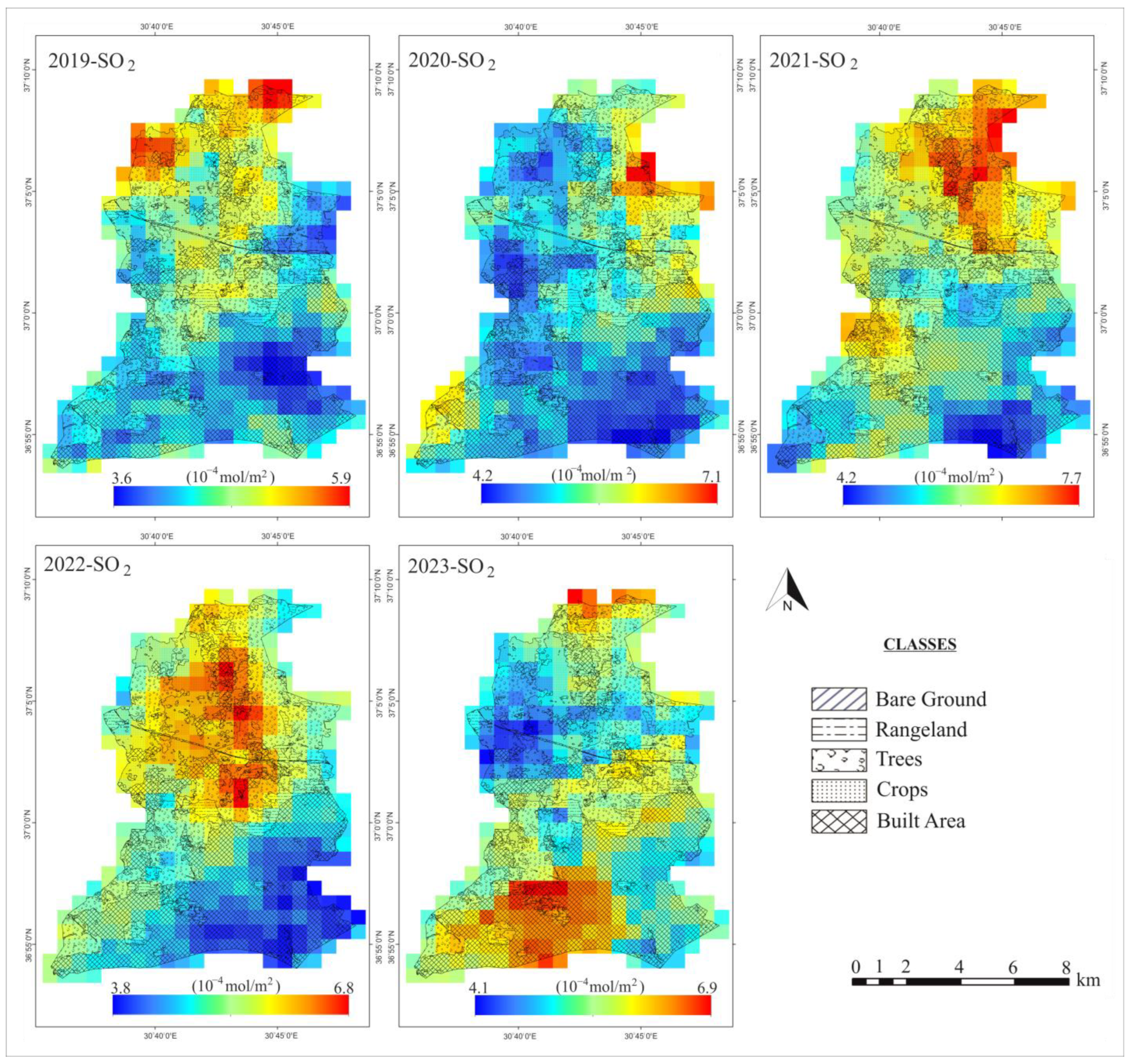
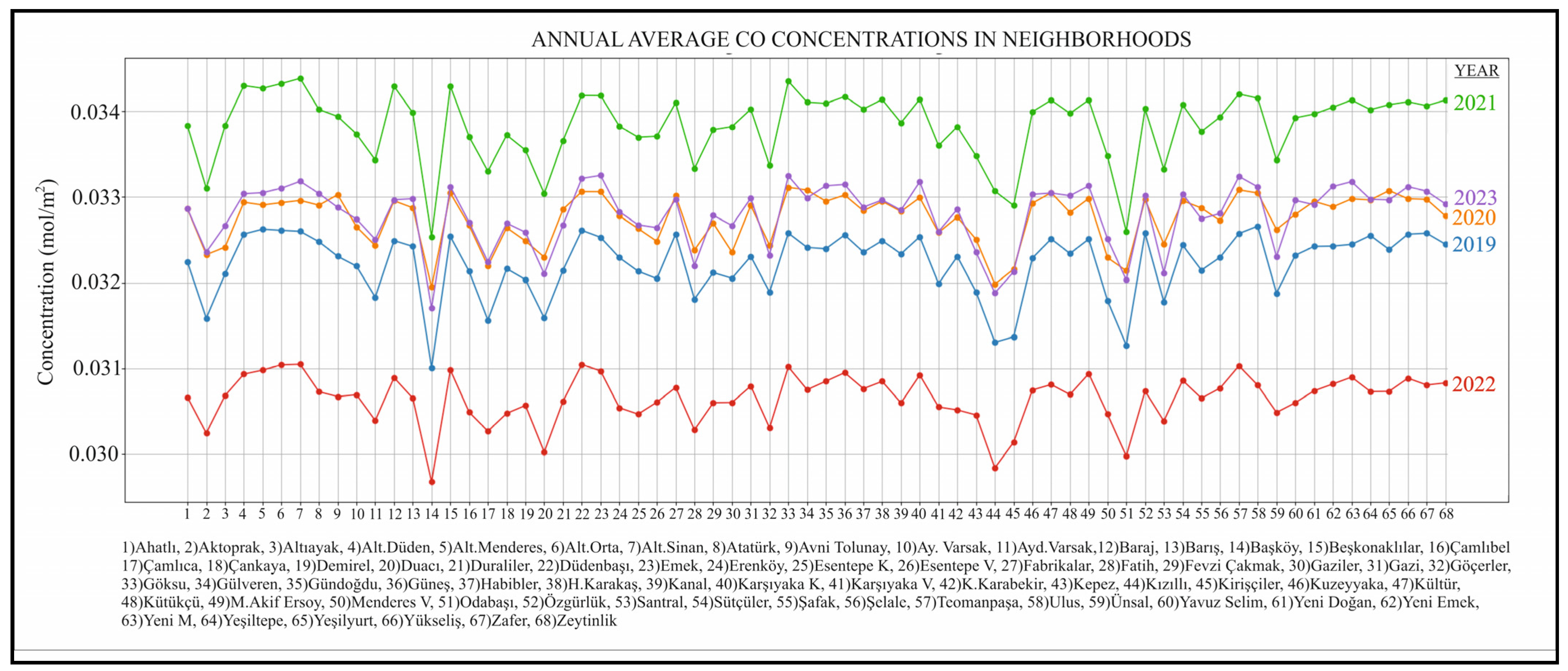
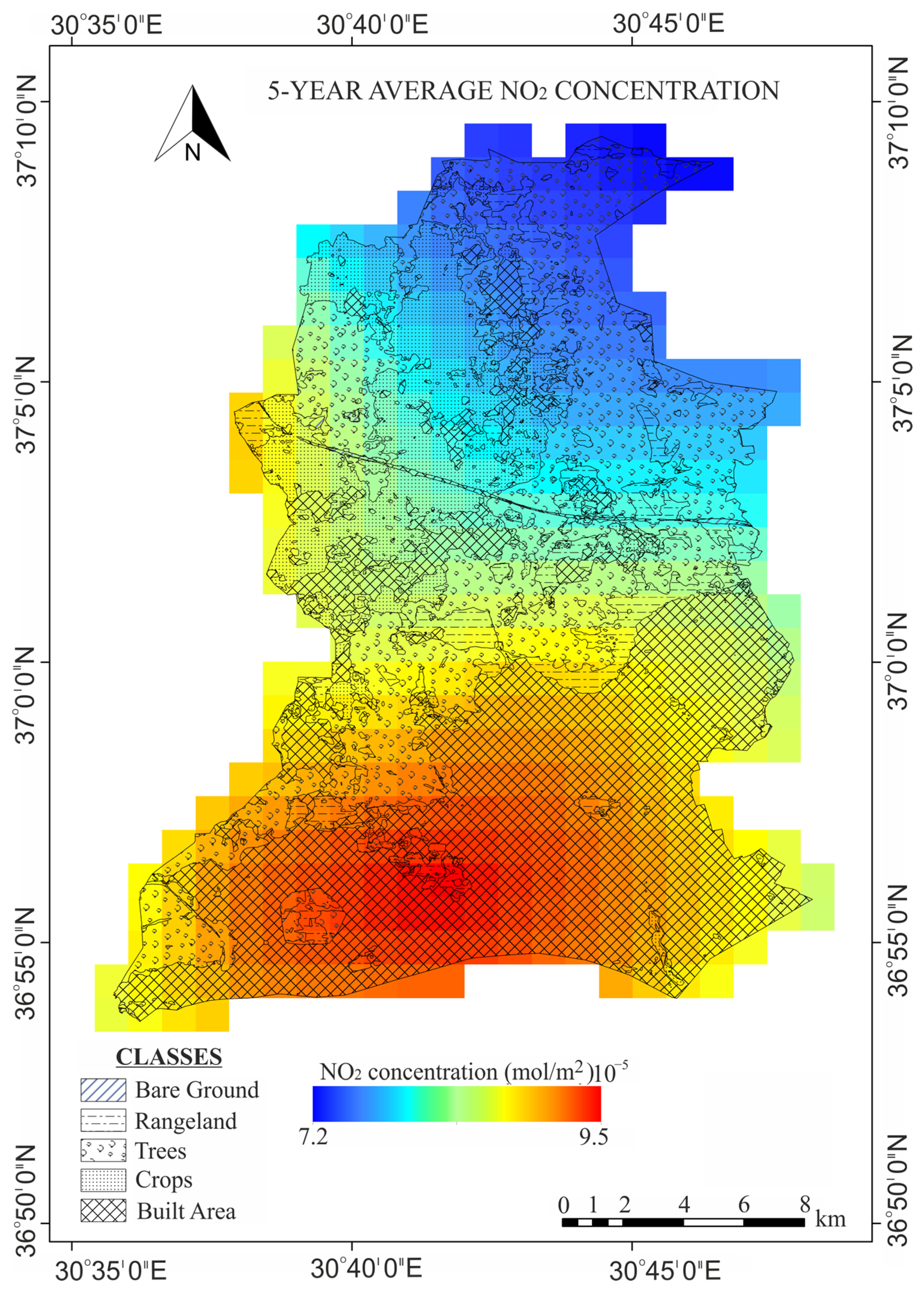
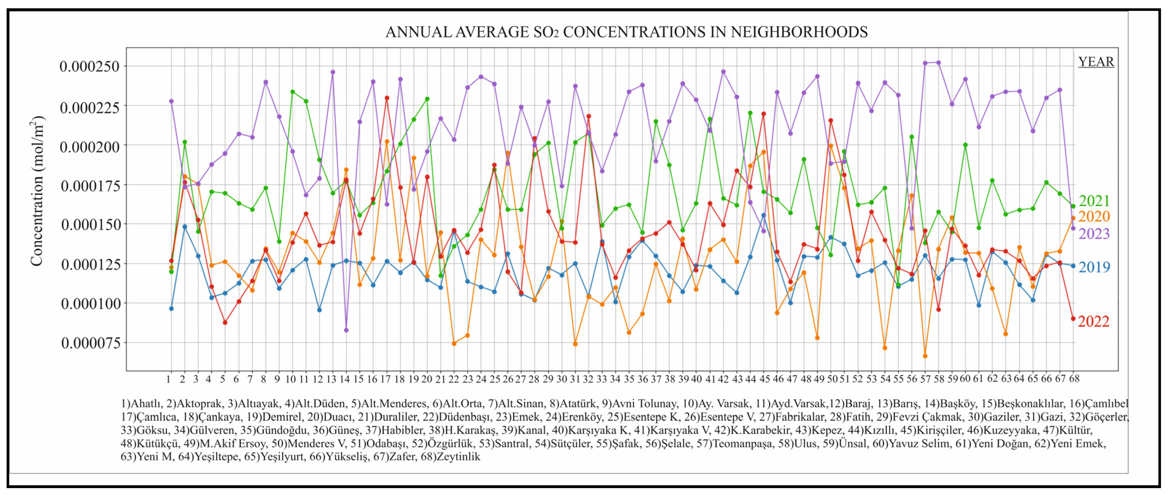
4.1. Air Pollutant Concentrations and Mapping
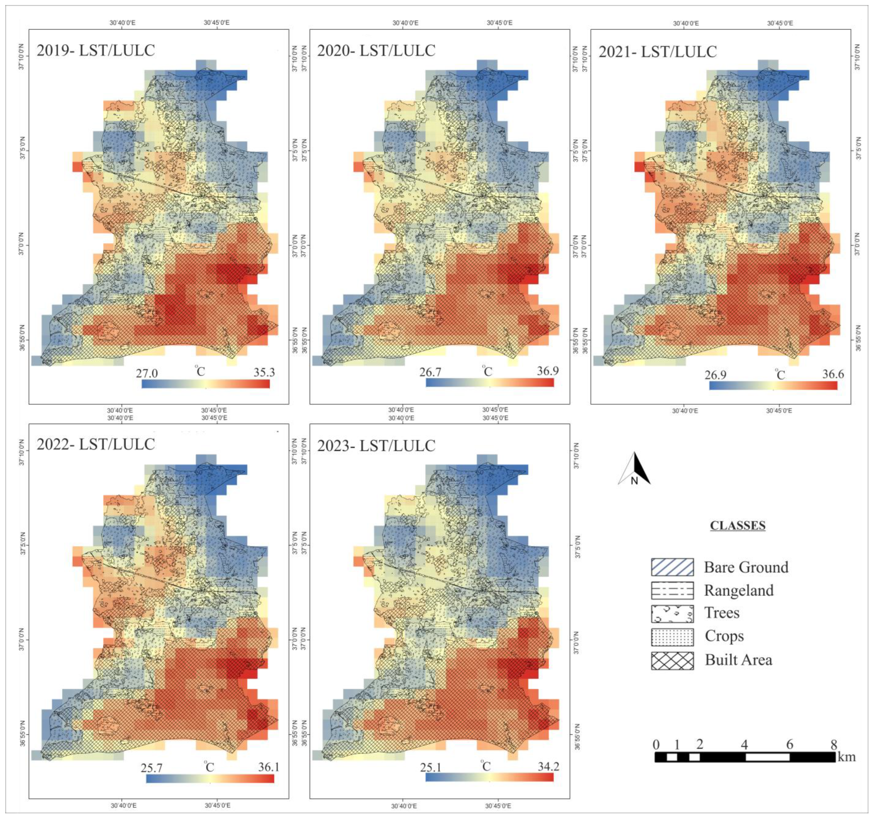
4.2. LST-LULC Maps
4.3. Integrated SVI Calculation and Mapping
5. Conclusions
Author Contributions
Funding
Institutional Review Board Statement
Informed Consent Statement
Data Availability Statement
Acknowledgments
Conflicts of Interest
Abbreviations
| RS | remote sensing |
| GIS | Geographic Information Systems |
| SVI | Social Vulnerability Index |
| LULC | Land Use Land Cover |
| TROPOMI | Tropospheric Monitoring Instrument |
| LST | Land Surface Temperature |
| PAH | polycyclic aromatic hydrocarbons |
| GEE | Google Earth Engine |
| PM | particulate matter |
| UV | ultraviolet |
| VIS | visible |
| NIR | near infrared |
| SWIR | shortwave infrared |
| QGIS | Quantum GIS |
| KMO | Kaiser–Meyer–Olkin |
| PAR | Pressure and Release model |
References
- Güllüdağ, C.B.; Kartal, N.Ü. Comparison of the distribution of environmentally hazardous elements in coal with Kriging and IDW methods (Tekirdağ-Malkara Coalfield). J. Sci. Rep.-A 2022, 50, 44–67. [Google Scholar]
- Daly, C. Air pollution and causes of death. Br. J. Prev. Soc. Med. 1959, 13, 14. [Google Scholar] [PubMed]
- Wu, X.; Braun, D.; Schwartz, J.; Kioumourtzoglou, M.A.; Dominici, F. Health and Medıcıne Evaluating the Impact of Long-Term Exposure to Fine Particulate Matter on Mortality among the Elderly. Sci. Adv. 2020, 6, eaba5692. [Google Scholar] [PubMed]
- Geldsetzer, P.; Fridljand, D.; Kiang, M.V.; Bendavid, E.; Heft-Neal, S.; Burke, M.; Thieme, A.H.; Benmarhnia, T. Disparities in Air Pollution Attributable Mortality in the US Population by Race/Ethnicity and Sociodemographic Factors. Nat. Med. 2024, 30, 2821–2829. [Google Scholar] [CrossRef]
- Available online: https://www.unep.org/news-and-stories/press-release/7-million-deaths-annually-linked-air-pollution-who-report (accessed on 20 November 2024).
- Phillips, D.I.W.; Osmond, C.; Southall, H.; Aucott, P.; Jones, A.; Holgate, S.T. Evaluating the Long-Term Consequences of Air Pollution in Early Life: Geographical Correlations between Coal Consumption in 1951/1952 and Current Mortality in England and Wales. BMJ Open 2018, 8, e018231. [Google Scholar] [CrossRef]
- Guliyev, R.; Akgün, M. Ardahan’da Kullanılan Kömürün Hava Kirliliğine Etkisinin Incelenmesi. Balıkesir Üniversitesi Fen Bilimleri Enstitüsü Dergisi 2020, 22, 479–489. [Google Scholar] [CrossRef]
- Li, X.; Yang, Y.; Xu, X.; Xu, C.; Hong, J. Air Pollution from Polycyclic Aromatic Hydrocarbons Generated by Human Activities and Their Health Effects in China. J. Clean. Prod. 2016, 112, 1360–1367. [Google Scholar] [CrossRef]
- Tayanc, M. An Assessment of Spatial and Temporal Variation of Sulfur Dioxide Levels over Istanbul, Turkey. Environ. Pollut. 2000, 107, 61–69. [Google Scholar]
- Qian, Z.; Chapman, R.S.; Tian, Q.; Chen, Y.; Lioy, P.J.; Zhang, J. Effects of Air Pollution on Children’s Respiratory Health in Three Chinese Cities. Arch. Environ. Health 2000, 55, 126–133. [Google Scholar] [CrossRef]
- Deng, M.; Ma, R.; Lu, F.; Nie, Y.; Li, P.; Ding, X.; Yuan, Y.; Shan, M.; Yang, X. Techno-Economic Performances of Clean Heating Solutions to Replace Raw Coal for Heating in Northern Rural China. Energy Build. 2021, 240, 110881. [Google Scholar] [CrossRef]
- Garipağaoğlu, N.D. Die Verteilung Luftverschmutzung Problemes Die İn Türkei Geographischegebieten. East. Geogr. Rev. 2011, 8. [Google Scholar]
- Pearce, J.; Kingham, S.; Zawar-Reza, P. Every Breath You Take? Environmental Justice and Air Pollution in Christchurch, New Zealand. Environ. Plan. A 2006, 38, 919–938. [Google Scholar] [CrossRef]
- Kaplan, G.; Avdan, Z.Y. Space-borne air pollution observation from sentinel-5p tropomi: Relationship between pollutants, geographical and demographic data. Int. J. Eng. Geosci. 2020, 5, 130–137. [Google Scholar] [CrossRef]
- Morozova, A.E.; Sizov, O.S.; Elagin, P.O.; Agzamov, N.A.; Fedash, A.V.; Lobzhanidze, N.E. Integral Assessment of Atmospheric Air Quality in the Largest Cities of Russia Based on TROPOMI (Sentinel-5P) Data for 2019–2020. Cosm. Res. 2022, 60, S57–S68. [Google Scholar] [CrossRef]
- Cersosimo, A.; Serio, C.; Masiello, G. TROPOMI NO2 Tropospheric Column Data: Regridding to 1 Km Grid-Resolution and Assessment of Their Consistency with in Situ Surface Observations. Remote Sens. 2020, 12, 2212. [Google Scholar] [CrossRef]
- Çakmak, N. Monitoring of NO2, CO and SO2 Gas Emissions with Sentinel-5P TROPOMI in Google Earth Engine Environment: Example of Marmara Region. Master’s Thesis, Yıldız Technical University, Istanbul, Turkey, 2022. [Google Scholar]
- Ceker, A.O. Investigatıon of the Change of NO2 Pollution during the Pandemic Period Using Satellite Retrievals in Marmara Region. Master’s Thesis, Technical University, Munich, Germany, 2022. [Google Scholar]
- Balamurugan, V.; Chen, J.; Qu, Z.; Bi, X.; Gensheimer, J.; Shekhar, A.; Bhattacharjee, S.; Keutsch, F.N. Tropospheric NO2 and O3 Response to COVID-19 Lockdown Restrictions at the National and Urban Scales in Germany. J. Geophys. Res. Atmos. 2021, 126. [Google Scholar] [CrossRef]
- Ialongo, I.; Virta, H.; Eskes, H.; Hovila, J.; Douros, J. Comparison of TROPOMI/Sentinel-5 Precursor NO2 Observations with Ground-Based Measurements in Helsinki. Atmos. Meas. Tech. 2020, 13, 205–218. [Google Scholar] [CrossRef]
- Makineci, H.B. Temporal Changes of NO2 and CO Emissions in Central Districts of Istanbul City. Turk. J. Remote Sens. 2022, 4, 62–74. [Google Scholar] [CrossRef]
- Sünsüli, M.; Kalkan, K. Sentinel-5p Uydu Görüntüleri İle Azot Dioksit (NO2) Kirliliğinin İzlenmesi. Turk. J. Remote Sens. 2022, 4, 1–6. [Google Scholar] [CrossRef]
- Karakoç, O. Creation of Çankırı Province Air Quality Map with Remote Sensing and Geographic Information Systems Integration. Master’s Thesis, Necmettin Erbakan University, Konya, Turkey, 2022. [Google Scholar]
- Aksoy, E. Meteorological Spatial Region Generation for Air Quality Specific to NO2 Using Remote Sensing and Ground Data: Ankara Case. Ph.D. Thesis, Akdeniz University, Antalya, Turkey, 2023. [Google Scholar]
- Ortakavak, Z. Sosyal Kırılganlık İndeksinin CBS Ile Haritalanması: İzmir İli Örneklemi. Resilience 2019, 3, 37–53. [Google Scholar] [CrossRef]
- Kuzucuoglu, A. Risk Management Strategy for Cultural Heritage. Mavhura ve Diğerleri (2017), an Approach for Measuring social Vulnerability in Context: The Case. 2013. Available online: https://www.researchgate.net/publication/281850036_RISK_MANAGEMENT_STRATEGY_FOR_CULTURAL_HERITAGE (accessed on 24 March 2025).
- Clarke, K.; Ash, K.; Coker, E.S.; Sabo-Attwood, T.; Bainomugisha, E. A Social Vulnerability Index for Air Pollution and Its Spatially Varying Relationship to PM2.5 in Uganda. Atmosphere 2022, 13, 1169. [Google Scholar] [CrossRef]
- Huang, G.; London, J. Mapping cumulative environmental effects, social vulnerability, and health in the San Joaquin Valley, California. Am. J. Public Health 2012, 102, 830–832. [Google Scholar] [PubMed]
- Bevan, G.; Pandey, A.; Griggs, S.; Dalton, J.E.; Zidar, D.; Patel, S.; Khan, S.U.; Nasir, K.; Rajagopalan, S.; Al-Kindi, S. Neighborhood-Level Social Vulnerability and Prevalence of Cardiovascular Risk Factors and Coronary Heart Disease. Curr. Probl. Cardiol. 2023, 48, 101182. [Google Scholar]
- Deziel, N.C.; Warren, J.L.; Bravo, M.A.; Macalintal, F.; Kimbro, R.T.; Bell, M.L. Assessing Community-Level Exposure to Social Vulnerability and Isolation: Spatial Patterning and Urban-Rural Differences. J. Expo. Sci. Environ. Epidemiol. 2023, 33, 198–206. [Google Scholar] [CrossRef]
- Bell, M.L.; Ebisu, K. Environmental Inequality in Exposures to Airborne Particulate Matter Components in the United States. Environ. Health Perspect. 2012, 120, 1699–1704. [Google Scholar]
- Hajat, A.; Diez-Roux, A.V.; Adar, S.D.; Auchincloss, A.H.; Lovasi, G.S.; O’Neill, M.S.; Sheppard, L.; Kaufman, J.D. Air Pollution and Individual and Neighborhood Socioeconomic Status: Evidence from the Multi-Ethnic Study of Atherosclerosis (MESA). Environ. Health Perspect. 2013, 121, 1325–1333. [Google Scholar] [CrossRef]
- Moore, J.; Evans, S.; Rose, C.E.; Shin, M.; Carroll, Y.; Duke, C.W.; Cohen, C.R.; Broussard, C.S. Increased Stillbirth Rates and Exposure to Environmental Risk Factors for Stillbirth in Counties with Higher Social Vulnerability: United States, 2015–2018. Matern. Child Health J. 2024, 28, 2026–2036. [Google Scholar] [CrossRef]
- Bell, M.L.; Dominici, F. Effect Modification by Community Characteristics on the Short-Term Effects of Ozone Exposure and Mortality in 98 US Communities. Am. J. Epidemiol. 2008, 167, 986–997. [Google Scholar] [CrossRef]
- Mennis, J.L.; Jordan, L. The Distribution of Environmental Equity: Exploring Spatial Nonstationarity in Multivariate Models of Air Toxic Releases. Ann. Assoc. Am. Geogr. 2005, 95, 249–268. [Google Scholar]
- Morello-Frosch, R.; Pastor, M. Envıronmental Justıce and Southern Calıfornıa’s “Rıskscape” the Distribution of Air Toxics Exposures and Health Risks Among Diverse Communities. Urban Aff. Rev. 2001, 36, 551–578. [Google Scholar]
- Miranda, M.L.; Edwards, S.E.; Keating, M.H.; Paul, C.J. Making the Environmental Justice Grade: The Relative Burden of Air Pollution Exposure in the United States. Int. J. Environ. Res. Public Health 2011, 8, 1755–1771. [Google Scholar] [CrossRef]
- McDonald, Y.J.; Jones, N.E. Drinking Water Violations and Environmental Justice in the United States, 2011–2015. Am. J. Public Health 2018, 108, 1401–1407. [Google Scholar] [CrossRef] [PubMed]
- Whitehead, L.S.; Buchanan, S.D. Childhood Lead poisoning: A perpetual environ- mental justice issue? J. Public Health Manag. Pract. 2019, 25, S115–S120. [Google Scholar] [CrossRef] [PubMed]
- Islam, S.J.; Malla, G.; Yeh, R.W.; Quyyumi, A.A.; Kazi, D.S.; Tian, W.; Song, Y.; Nayak, A.; Mehta, A.; Ko, Y.A.; et al. County-Level Social Vulnerability Is Associated with In-Hospital Death and Major Adverse Cardiovascular Events in Patients Hospitalized with COVID-19: An Analysis of the American Heart Association COVID-19 Cardiovascular Disease Registry. Circ. Cardiovasc. Qual. Outcomes 2022, 15, 611–619. [Google Scholar] [CrossRef]
- Ge, Y.; Zhang, H.; Dou, W.; Chen, W.; Liu, N.; Wang, Y.; Shi, Y.; Rao, W. Mapping Social Vulnerability to Air Pollution: A Case Study of the Yangtze River Delta Region, China. Sustainability 2017, 9, 109. [Google Scholar] [CrossRef]
- Özgürel, Y. Temporal and Spatial Evaluation of Fossil Fuel Sourced Air Pollutants Using Remote Sensing and Terrestrial Data: Antalya İli Kepez Sample. Master’s Thesis, Akdeniz University, Antalya, Turkey, 2024. [Google Scholar]
- Kepez District Governorship. Kepez District Governorship Official Website. 2024. Available online: http://www.kepez.gov.tr/ (accessed on 22 November 2024).
- Türkmen, S.; Kalağan, G. Türkiye’de yoksullukla mücadelede yerel yönetimlerin rolü: Antalya Kepez belediyesi örneği. Oğuzhan Sosyal Bilimler Dergisi 2023, 5, 125–142. [Google Scholar] [CrossRef]
- GEE. 2024. Available online: https://code.earthengine.google.com/ (accessed on 10 November 2024).
- Esri-Sentinel 2 LULC. 2023. Available online: https://livingatlas.arcgis.com/landcoverexplorer/ (accessed on 5 September 2024).
- Cutter, S.L.; Mitchell, J.T.; Scott, M.S. Revealing the Vulnerability of People and Places: A Case Study of Georgetown County, South Carolina. Ann. Assoc. Am. Geogr. 2000, 90, 713–737. [Google Scholar] [CrossRef]
- Fekete, A. Validation of a Social Vulnerability Index in Context to River-Floods in Germany. Nat. Hazards Earth Syst. Sci. 2009, 9, 393–403. [Google Scholar] [CrossRef]
- Cutter, S.L.; Boruff, B.J.; Shirley, W.L. Social vulnerability to environmental hazards. Soc. Sci. Q. 2003, 84, 242–261. [Google Scholar] [CrossRef]
- Kirby, R.H.; Reams, M.A.; Lam, N.S.N.; Zou, L.; Dekker, G.G.J.; Fundter, D.Q.P. Assessing Social Vulnerability to Flood Hazards in the Dutch Province of Zeeland. Int. J. Disaster Risk Sci. 2019, 10, 233–243. [Google Scholar] [CrossRef]
- Karra, K. Global land use/land cover with Sentinel-2 and deep learning. In Proceedings of the IGARSS 2021-2021 IEEE International Geoscience and Remote Sensing Symposium, Brussels, Belgium, 11–16 July 2021; IEEE: Piscataway, NJ, USA, 2021. [Google Scholar]
- NSIDC. National Snow and Ice Data Centre Website. 2024. Available online: https://nsidc.org/data/modis (accessed on 8 October 2024).
- Parida, B.R.; Bar, S.; Roberts, G.; Mandal, S.P.; Pandey, A.C.; Kumar, M.; Dash, J. Improvement in air quality and its impact on land surface temperature in major urban areas across India during the first lockdown of the pandemic. Environ. Res. 2021, 199, 111280. [Google Scholar] [CrossRef]
- Wan, Z.; Dozier, J. A generalized split-window algorithm for retrieving landsurface temperature from space. IEEE Trans. Geosci. Rem. Sens. 1996, 34, 892–905. [Google Scholar]
- Li, Z.L.; Tang, B.H.; Wu, H.; Ren, H.; Yan, G.; Wan, Z.; Trigo, I.F.; Sobrino, J.A. Satellite-derived land surface temperature: Current status and perspectives. Remote Sens. Environ. 2013, 131, 14–37. [Google Scholar] [CrossRef]
- Liu, X.; Li, Z.-L.; Li, J.-H.; Leng, P.; Liu, M.; Gao, M. Temporal upscaling of MODIS 1-km ınstantaneous Land Surface Temperature to monthly mean value: Method evaluation and product generation. IEEE Trans. Geosci. Remote Sens. 2023, 61, 1–14. [Google Scholar] [CrossRef]
- Demir, E. R Diliyle İstatistik Uygulamaları; Pegem Akademi: Ankara, Turkey, 2019. [Google Scholar]
- Crawley, M.J. Statistics: An İntroduction Using R; John Wiley & Sons: Hoboken, NJ, USA, 2014. [Google Scholar]
- Khemka, A. A Colloborative Predictive Data Mining Model. Master’s Thesis, University of Missouri, Kansas City, MO, USA, 2003. [Google Scholar]
- Nakip, M. Pazarlama Araştırmaları Teknikler ve (SPSS Destekli) Uygulamalar; Seçkin Yayıncılık: Ankara, Turkey, 2003. [Google Scholar]
- Wisner, B.; Blaikie, P.; Cannon, T.; Davis, I. At Risk. Natural Hazards, People’s Vulnerability and Disasters, 2nd ed.; Routledge: London, UK, 2004. [Google Scholar]
- Yang, X.; Geng, L.; Zhou, K. Environmental pollution, income growth, and subjective well-being: Regional and individual evidence from China. Environ. Sci. Pollut. Res. Int. 2020, 27, 34211–34222. [Google Scholar] [CrossRef] [PubMed]
- Hakovirta, M. Socioeconomic Aspects of Climate Change in Cities and Municipalities. In Carbon Neutrality. Springer Climate; Springer: Cham, Switzerland, 2023. [Google Scholar] [CrossRef]
- Garlick, D. The vulnerable people in emergencies policy: Hiding vulnerable people in plain sight. Aust. J. Emerg. Manag. 2015, 30, 31–34. [Google Scholar]
- Son, J.-Y.; Muenich, R.L.; Schaffer-Smith, D.; Miranda, M.L.; Bell, M.L. Distribution of environmental justice metrics for exposure to CAFOs in North Carolina, USA. Environ. Res. 2021, 195, 110862. [Google Scholar] [CrossRef]
- Wing, S.; Cole, D.; Grant, G. Environmental injustice in North Carolina’s hog industry. Environ. Health Perspect. 2000, 108, 225–231. [Google Scholar]
- Silva, G.S.; Warren, J.L.; Deziel, N.C. Spatial modelling to identify sociodemographic predictors of hydraulic fracturing wastewater injection wells in Ohio census block groups. Environ. Health Perspect. 2018, 126, 067008. [Google Scholar] [CrossRef]


| Process | Source | Platform | Data | Resolution (m) | Data Type | Year | Unit |
|---|---|---|---|---|---|---|---|
| RS (Remote Sensing) | Google Earth Engine [45] | Sentinel-5P TROPOMI | CO | 1113.2 | Raster Data | 2019–2023 | mol/m2 |
| NO2 | |||||||
| SO2 | |||||||
| Terra and Aqua MODIS | LST | 1000 | °C | ||||
| ESRI (Living Atlas of the World) [46] | Sentinel-2 | LULC | 10 | 2023 | - | ||
| Process | Source | Data | Classification | Data Type | Reference [25] | ||
| SVI (Social Vulnerability Index) | Turkish Statistical Institute (data taken between 2019–2023) | Population density | Person/km2 | Text and number | [47] | ||
| Households | Population per household | [48] | |||||
| Marital status (Female/Male separately) | Never married | [25] | |||||
| Married | |||||||
| Divorced | |||||||
| Dead | |||||||
| Age | <15 | [49,50] | |||||
| +65 | |||||||
| Gender | Woman | [49] | |||||
| Male | |||||||
| Education | Illiterate | ||||||
| Primary school graduate | |||||||
| Secondary school graduate | |||||||
| High school graduate | |||||||
| Graduate of Higher School/Faculty | |||||||
| Master’s degree graduate | |||||||
| Band | Spectral Coverage (nm) | Span (km) | Spectral Resolution (nm) | Temporal Resolution | Spatial Resolution (km2) | |
|---|---|---|---|---|---|---|
| UV | 1 | 270–320 | 2600 | 0.49 | Diary | 7 × 28 |
| 2 | 7 × 3.5 | |||||
| VIS | 3 | 320–495 | 0.54 | |||
| 4 | ||||||
| NIR | 5 | 675–775 | 0.38 | |||
| 6 | ||||||
| SWIR | 7 | 2305–2385 | 0.25 | 7 × 7 | ||
| 8 | ||||||
| Air Pollutant | Highest Value | Lowest Value | ||
|---|---|---|---|---|
| 5-Year High Value | Year Observed | 5-Year Low Value | Year Observed | |
| CO | 32.4 × 10⁻³ mol/m2–34.4 × 10−3 mol/m2/2021 | 2021 | 29.4 × 10⁻³ mol/m2–31.1 × 10−3 mol/m2/2022 | 2022 |
| SO2 | 4.2 × 10⁻⁴ mol/m2–7.7 × 10−4 mol/m2/2021 | 2021 | 3.6 × 10⁻⁴ mol/m2–5.9 × 10−4 mol/m2/2019 | 2019 |
| NO2 | 7.4 × 10⁻⁵ mol/m2–10.2 × 10−5 mol/m2/2023 | 2023 | 6.7 × 10⁻⁵ mol/m2–8.6 × 10−5 mol/m2/2020 | 2020 |
| Variable | Factor | Initial Eigenvalues | Values After Factorization | ||||||||
|---|---|---|---|---|---|---|---|---|---|---|---|
| 1 | 2 | 3 | Factor | Total | Variance % | Cumulative % | Factor | Total | % Variance | Cumulative % | |
| Illiterate Population | 0.937 | 0.062 | 0.118 | 1 | 10.193 | 63.706 | 63.706 | 1 | 10.193 | 63.706 | 63.706 |
| Secondary School Graduate | 0.929 | 0.322 | 0.107 | 2 | 2.296 | 14.349 | 78.055 | ||||
| Under 15 Years Old Population | 0.911 | 0.347 | 0.048 | 3 | 1.388 | 8.677 | 86.732 | ||||
| Primary School Graduates Population | 0.903 | 0.395 | 0.112 | 4 | 0.776 | 4.849 | 91.581 | ||||
| Female Population | 0.832 | 0.542 | 0.056 | 5 | 0.514 | 3.213 | 94.795 | ||||
| Household Population | 0.746 | 0.647 | −0.027 | 6 | 0.296 | 1.851 | 96.645 | ||||
| High School Graduate | 0.701 | 0.698 | 0.046 | 7 | 0.221 | 1.38 | 98.025 | ||||
| Higher School Graduate | 0.373 | 0.895 | −0.101 | 8 | 0.144 | 0.899 | 98.925 | 2 | 2.296 | 14.349 | 78.055 |
| Master’s Degree | 0.05 | 0.841 | −0.347 | 9 | 0.079 | 0.494 | 99.418 | ||||
| Over 65 Years of Age Population | 0.445 | 0.756 | 0.139 | 10 | 0.047 | 0.291 | 99.71 | ||||
| Divorced Population | 0.598 | 0.754 | 0.066 | 11 | 0.022 | 0.135 | 99.845 | ||||
| Population Density | 0.27 | 0.736 | 0.307 | 12 | 0.01 | 0.065 | 99.91 | ||||
| Spouse Deceased Population | 0.631 | 0.698 | 0.193 | 13 | 0.006 | 0.04 | 99.95 | ||||
| CO | 0.006 | 0.054 | 0.907 | 14 | 0.005 | 0.03 | 99.98 | 3 | 1.388 | 8.677 | 86.732 |
| SO2 | −0.195 | −0.06 | −0.791 | 15 | 0.002 | 0.011 | 99.99 | ||||
| NO2 | 0.019 | −0.064 | 0.7 | 16 | 0.002 | 0.01 | 100 | ||||
| Neighborhood Name | Factor 1 | Factor 2 | Factor 3 | Integrated SVI | Neighborhood Name | Factor 1 | Factor 2 | Factor 3 | Integrated SVI |
|---|---|---|---|---|---|---|---|---|---|
| Ahatlı | 0.93 | 1.11 | 0.35 | 2.39 | Habibler | 1.56 | 0.42 | 0.37 | 2.34 |
| Aktoprak | 0.34 | −0.03 | 0.06 | 0.36 | Hüsnü Karakaş | 1.44 | 0.40 | 0.35 | 2.19 |
| Altıayak | −0.81 | −0.87 | 0.18 | −1.50 | Kanal | 0.41 | 0.62 | 0.29 | 1.32 |
| Alt. Düden | −0.71 | −0.68 | 0.35 | −1.05 | Karşıyaka | 0.93 | 0.95 | 0.33 | 2.21 |
| Altınova Orta | −0.24 | −0.33 | 0.33 | −0.24 | Kazım Karabekir | −0.98 | −0.78 | 0.33 | −1.43 |
| Altınova Sinan | −0.38 | −0.52 | 0.33 | −0.58 | Kepez | −0.85 | −0.38 | 0.38 | −0.85 |
| Atatürk | −0.16 | 0.41 | 0.32 | 0.57 | Kızıllı | −0.96 | −0.89 | 0.21 | −1.64 |
| Avni Tolunay | −0.76 | −0.58 | 0.33 | −1.01 | Kirişçiler | −1.08 | −0.95 | 0.30 | −1.74 |
| Ayanoğlu | 0.24 | −0.05 | 0.32 | 0.51 | Kuzeyyaka | 2.26 | 1.07 | 0.21 | 3.54 |
| Aydoğmuş | 0.41 | 0.12 | 0.25 | 0.78 | Kültür | 0.48 | 1.63 | −0.06 | 2.06 |
| Baraj | 0.10 | −0.36 | 0.16 | −0.09 | Kütükçü | −0.23 | −0.10 | 0.05 | −0.27 |
| Barış | −0.26 | −0.10 | 0.35 | −0.01 | M. Akif Ersoy | 0.54 | 0.20 | 0.35 | 1.09 |
| Başköy | −1.14 | −1.00 | 0.32 | −1.82 | Menderes | −0.78 | −0.81 | 0.37 | −1.21 |
| Beşkonaklılar | −0.82 | −0.79 | 0.18 | −1.44 | Odabaşı | −1.11 | −0.95 | 0.32 | −1.74 |
| Çamlıbel | −0.24 | −0.11 | 0.34 | −0.01 | Özgürlük | 0.40 | 1.49 | 0.37 | 2.26 |
| Çamlıca | −1.05 | −0.73 | 0.27 | −1.51 | Santral | −1.16 | −0.86 | 0.09 | −1.93 |
| Çankaya | 0.13 | 0.80 | −0.03 | 0.90 | Sütçüler | 0.16 | −0.05 | −0.04 | 0.07 |
| Demirel | −0.75 | −0.71 | 0.25 | −1.22 | Şafak | 1.10 | 0.36 | 0.35 | 1.80 |
| Duacı | −0.92 | −0.48 | 0.18 | −1.21 | Şelale | 0.57 | −0.11 | 0.16 | 0.63 |
| Duraliler | −0.76 | −0.48 | 0.09 | −1.15 | Teomanpaşa | 2.03 | 1.07 | 0.35 | 3.46 |
| Düdenbaşı | 1.23 | 0.54 | 0.25 | 2.03 | Ulus | 0.55 | 1.59 | 0.31 | 2.46 |
| Emek | 0.13 | 0.21 | 0.37 | 0.70 | Ünsal | 0.50 | 0.12 | 0.28 | 0.90 |
| Erenköy | 0.39 | 0.41 | 0.40 | 1.20 | Varsak Esentepe | −1.02 | −0.92 | 0.38 | −1.56 |
| Esentepe | −0.37 | −0.33 | 0.31 | −0.39 | Varsak Karşıyaka | 0.40 | 0.16 | 0.37 | 0.93 |
| Fabrikalar | −0.07 | 0.38 | 0.25 | 0.57 | Varsak Menderes | −1.00 | −0.95 | 0.18 | −1.77 |
| Fatih | −0.37 | −0.37 | 0.20 | −0.55 | Yavuz Selim | −0.97 | −0.80 | 0.30 | −1.47 |
| Fevzi Çakmak | 0.35 | 0.13 | 0.36 | 0.85 | Yeni | 0.63 | 0.50 | 0.36 | 1.49 |
| Gazi | 0.59 | 0.22 | 0.18 | 0.98 | Yeni Doğan | −0.08 | 0.59 | 0.34 | 0.85 |
| Gaziler | −0.70 | −0.84 | 0.27 | −1.27 | Yeni Emek | 0.74 | 0.46 | 0.38 | 1.58 |
| Göçerler | −0.19 | −0.40 | 0.33 | −0.26 | Yeşiltepe | 0.17 | 0.94 | 0.35 | 1.46 |
| Göksu | −0.23 | −0.09 | 0.17 | −0.15 | Yeşilyurt | 0.17 | 0.50 | 0.35 | 1.02 |
| Gülveren | −0.62 | −0.22 | 0.18 | −0.66 | Yükseliş | −0.03 | 0.46 | 0.35 | 0.78 |
| Gündoğdu | 0.99 | 0.59 | 0.35 | 1.93 | Zafer | −0.24 | 0.67 | 0.35 | 0.78 |
| Güneş | 1.64 | 0.23 | 0.36 | 2.22 | Zeytinlik | −0.46 | −0.70 | 0.30 | −0.85 |
| Variable | Number of Neighborhoods Belonging to Classes | ||||
|---|---|---|---|---|---|
| Very High | High | Moderate | Low | Very Low | |
| Factor-1 | 14 | 12 | 13 | 15 | 14 |
| Factor-2 | 14 | 13 | 14 | 13 | 14 |
| Factor-3 | 12 | 14 | 15 | 10 | 17 |
| Integrated SVI | 14 | 12 | 15 | 13 | 14 |
Disclaimer/Publisher’s Note: The statements, opinions and data contained in all publications are solely those of the individual author(s) and contributor(s) and not of MDPI and/or the editor(s). MDPI and/or the editor(s) disclaim responsibility for any injury to people or property resulting from any ideas, methods, instructions or products referred to in the content. |
© 2025 by the authors. Licensee MDPI, Basel, Switzerland. This article is an open access article distributed under the terms and conditions of the Creative Commons Attribution (CC BY) license (https://creativecommons.org/licenses/by/4.0/).
Share and Cite
Güllüdağ, B.; Aksoy, E.; Özgürel, Y. Remote Sensing and Geographic Information Systems Detection of Fossil Fuel Air Pollution Impact in Socially Fragile Areas. Sustainability 2025, 17, 3031. https://doi.org/10.3390/su17073031
Güllüdağ B, Aksoy E, Özgürel Y. Remote Sensing and Geographic Information Systems Detection of Fossil Fuel Air Pollution Impact in Socially Fragile Areas. Sustainability. 2025; 17(7):3031. https://doi.org/10.3390/su17073031
Chicago/Turabian StyleGüllüdağ, Bertan, Ercüment Aksoy, and Yusuf Özgürel. 2025. "Remote Sensing and Geographic Information Systems Detection of Fossil Fuel Air Pollution Impact in Socially Fragile Areas" Sustainability 17, no. 7: 3031. https://doi.org/10.3390/su17073031
APA StyleGüllüdağ, B., Aksoy, E., & Özgürel, Y. (2025). Remote Sensing and Geographic Information Systems Detection of Fossil Fuel Air Pollution Impact in Socially Fragile Areas. Sustainability, 17(7), 3031. https://doi.org/10.3390/su17073031