
Monitoring and Evaluation of Ecological Restoration Effectiveness: A Case Study of the Liaohe River Estuary Wetland

 and
and
Abstract
1. Introduction
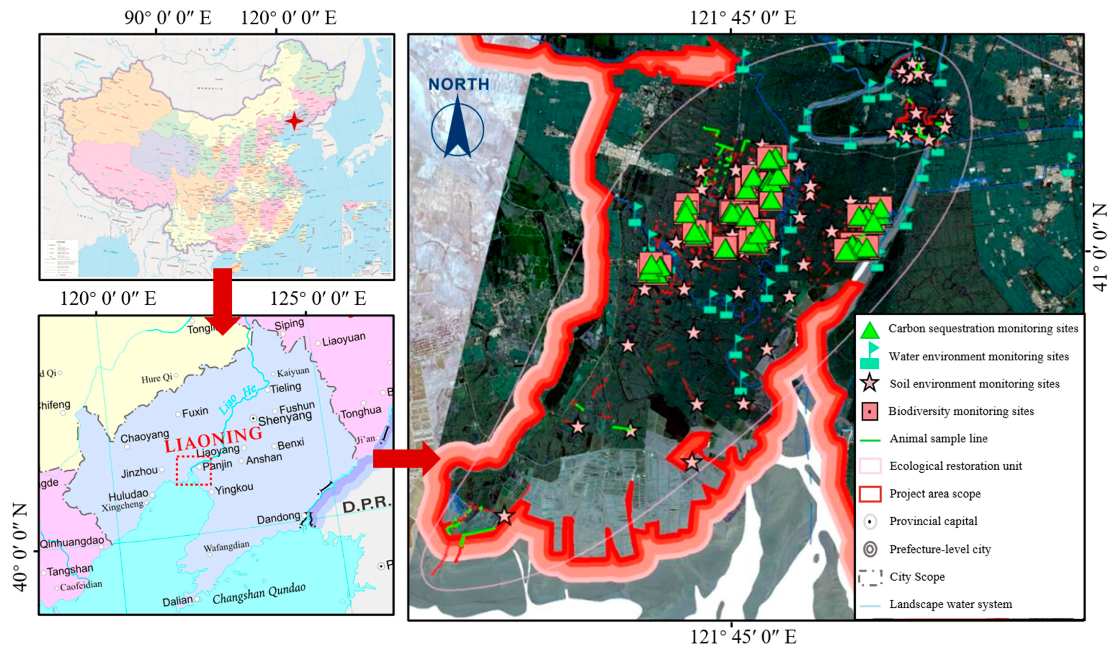
2. Study Area and Data
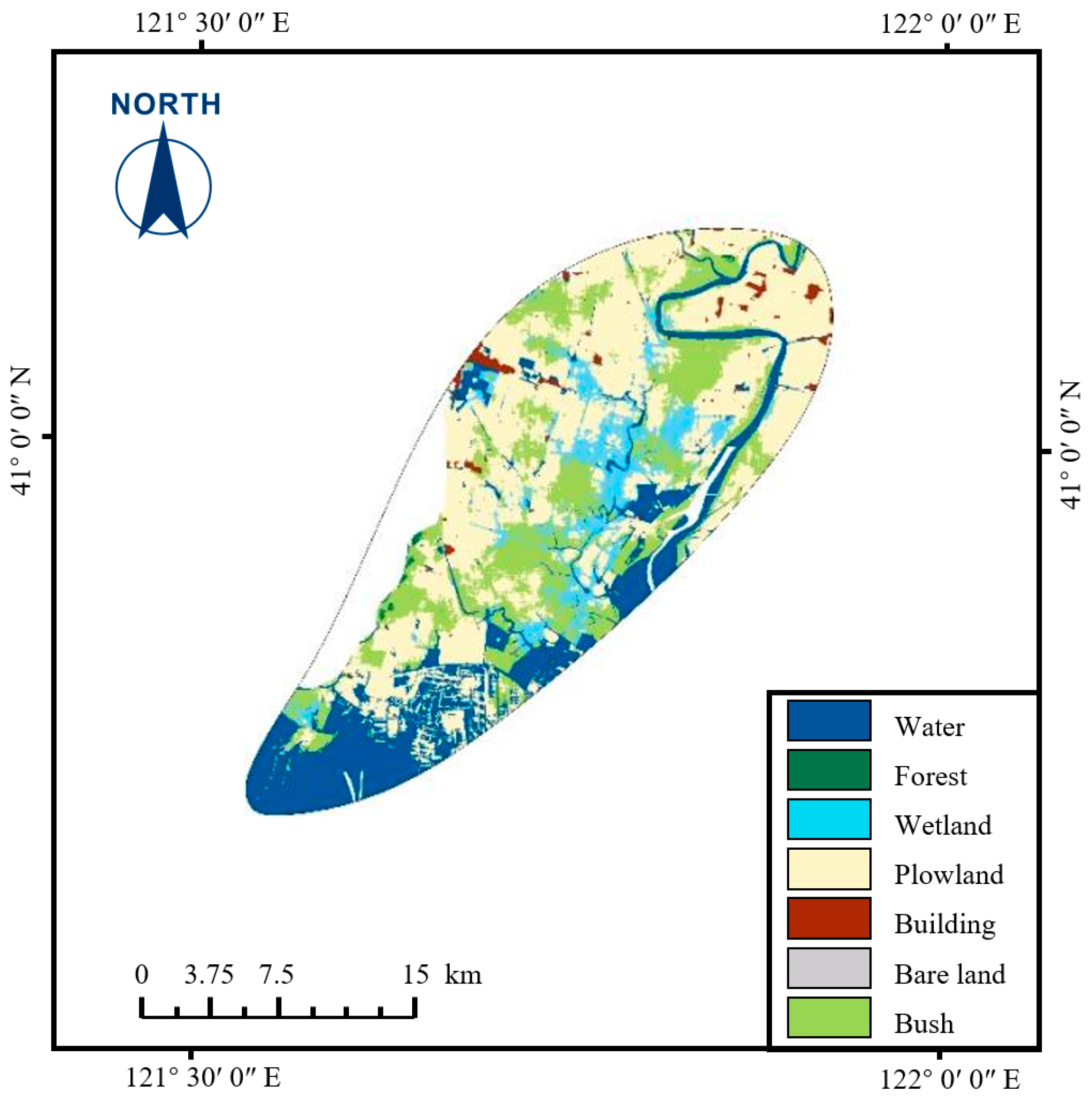
2.1. Overview of the Study Area
2.2. Data Sources
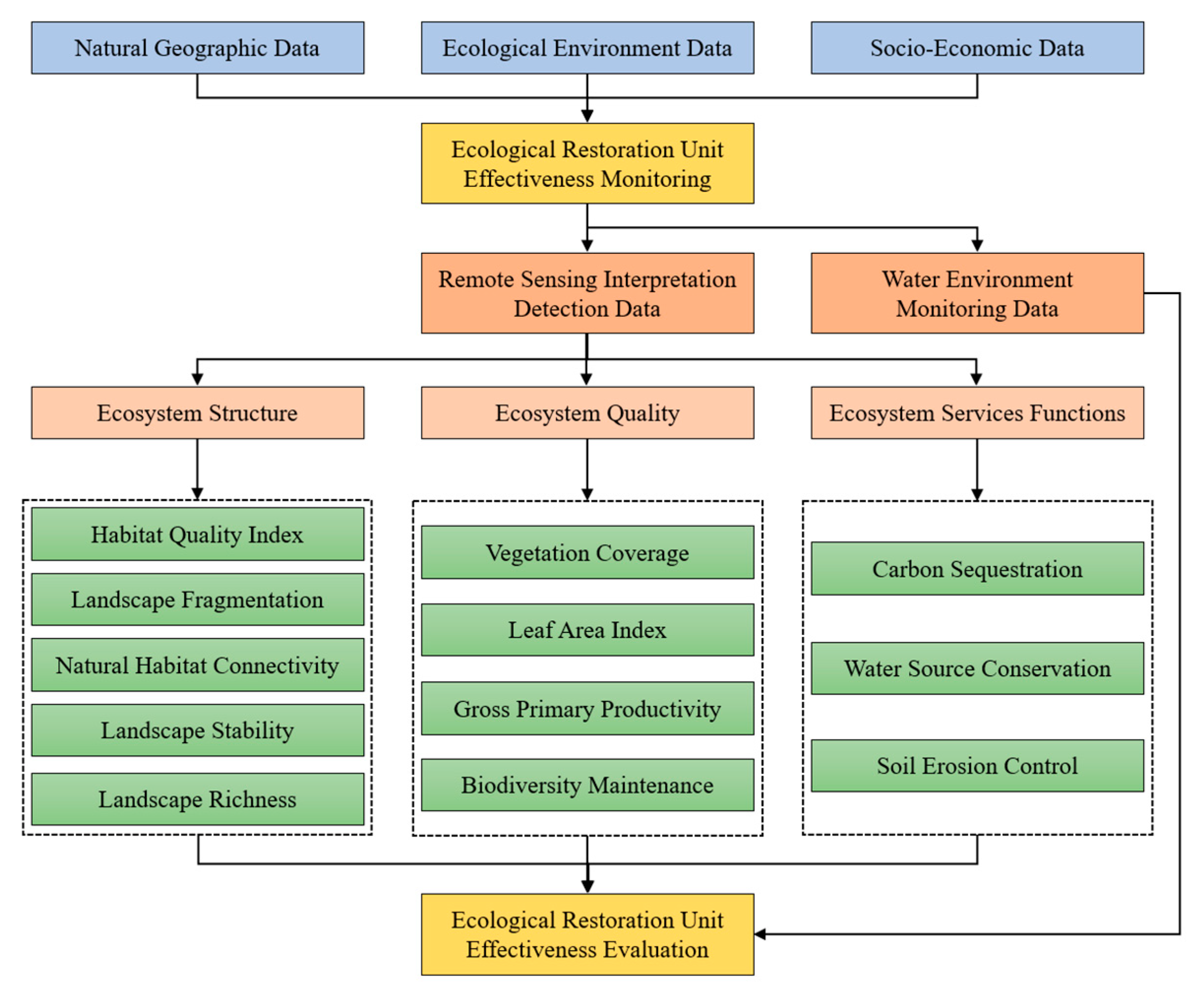
3. Methods
3.1. Water Environment Evaluation Method
3.2. Ecosystem Structure Evaluation Method
3.3. Ecological Environment Quality Evaluation Method
3.4. Ecosystem Service Function Evaluation Method
4. Results
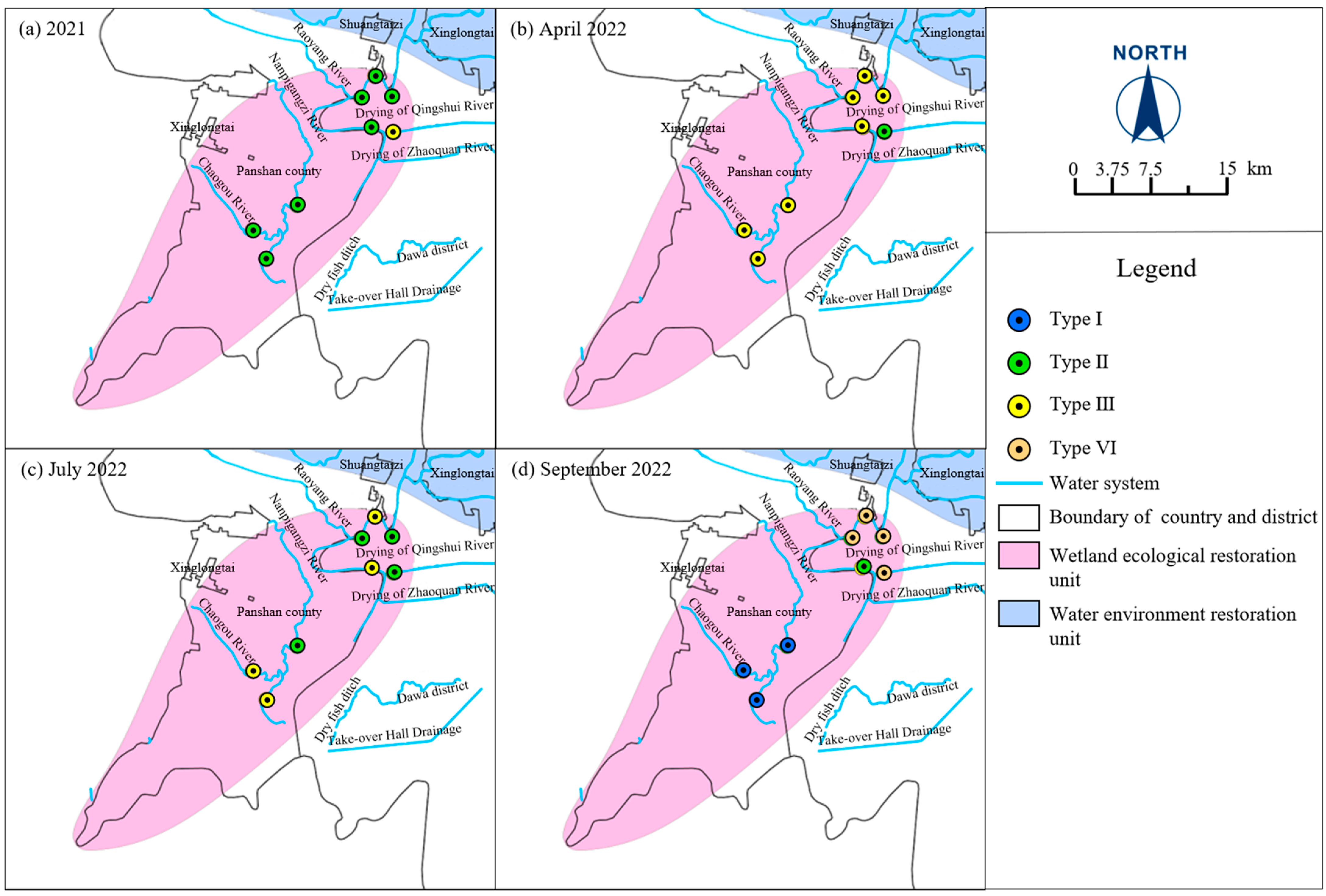
4.1. Water Environment Evaluation Results
4.2. Ecosystem Landscape Structure Evaluation Results
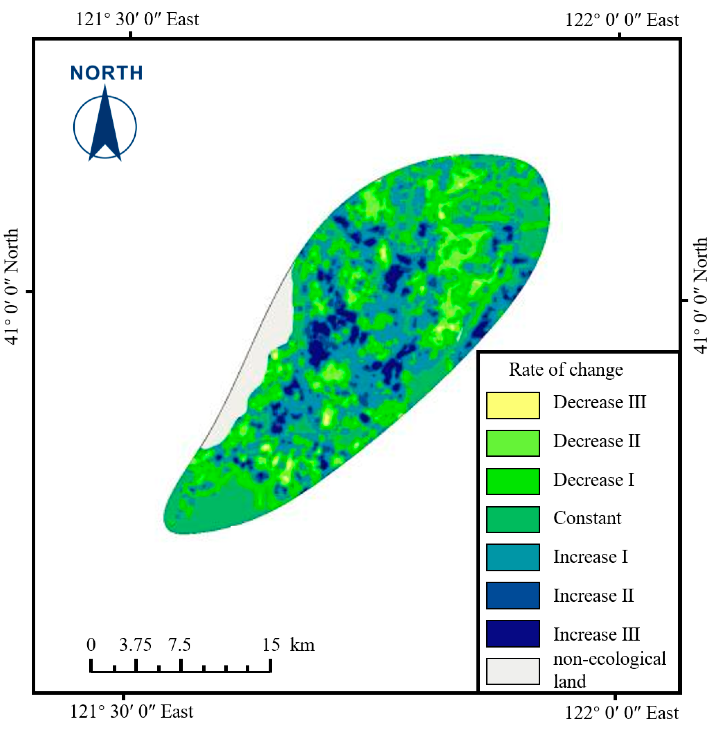
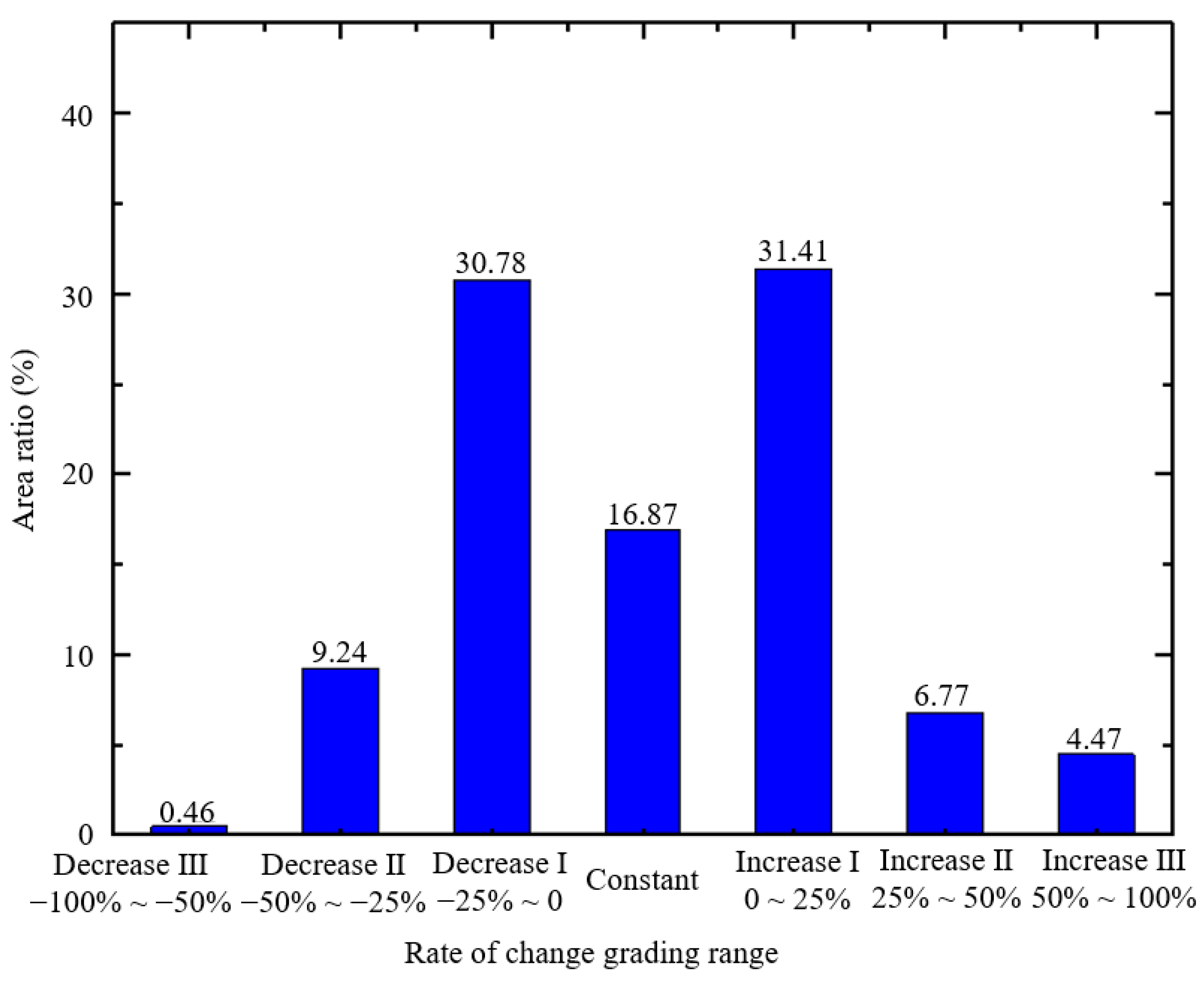
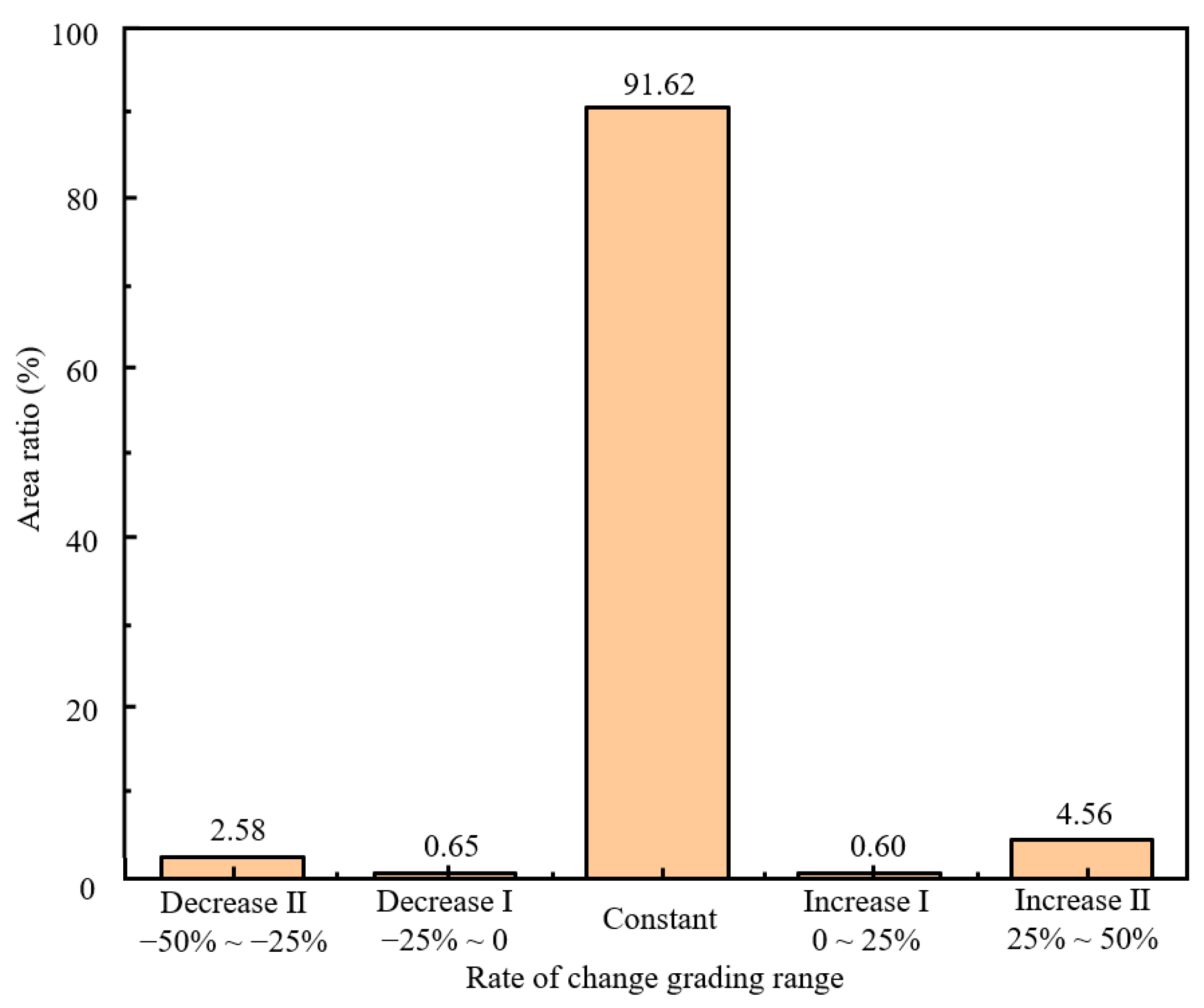
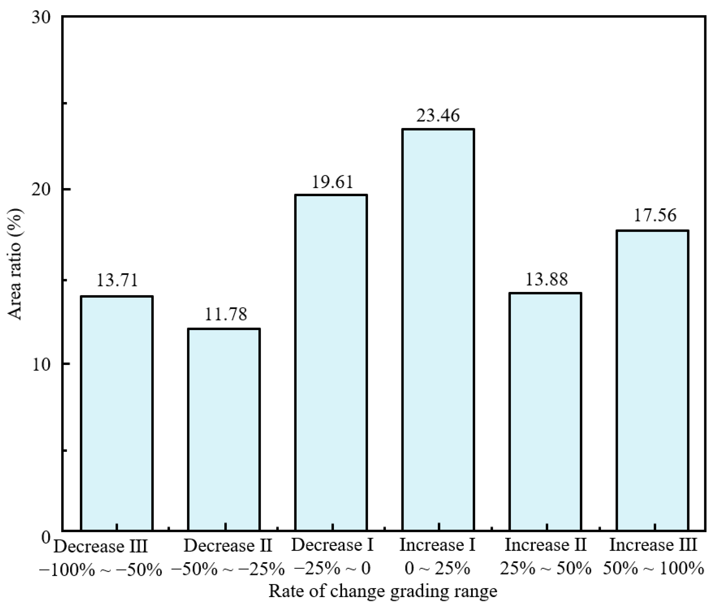
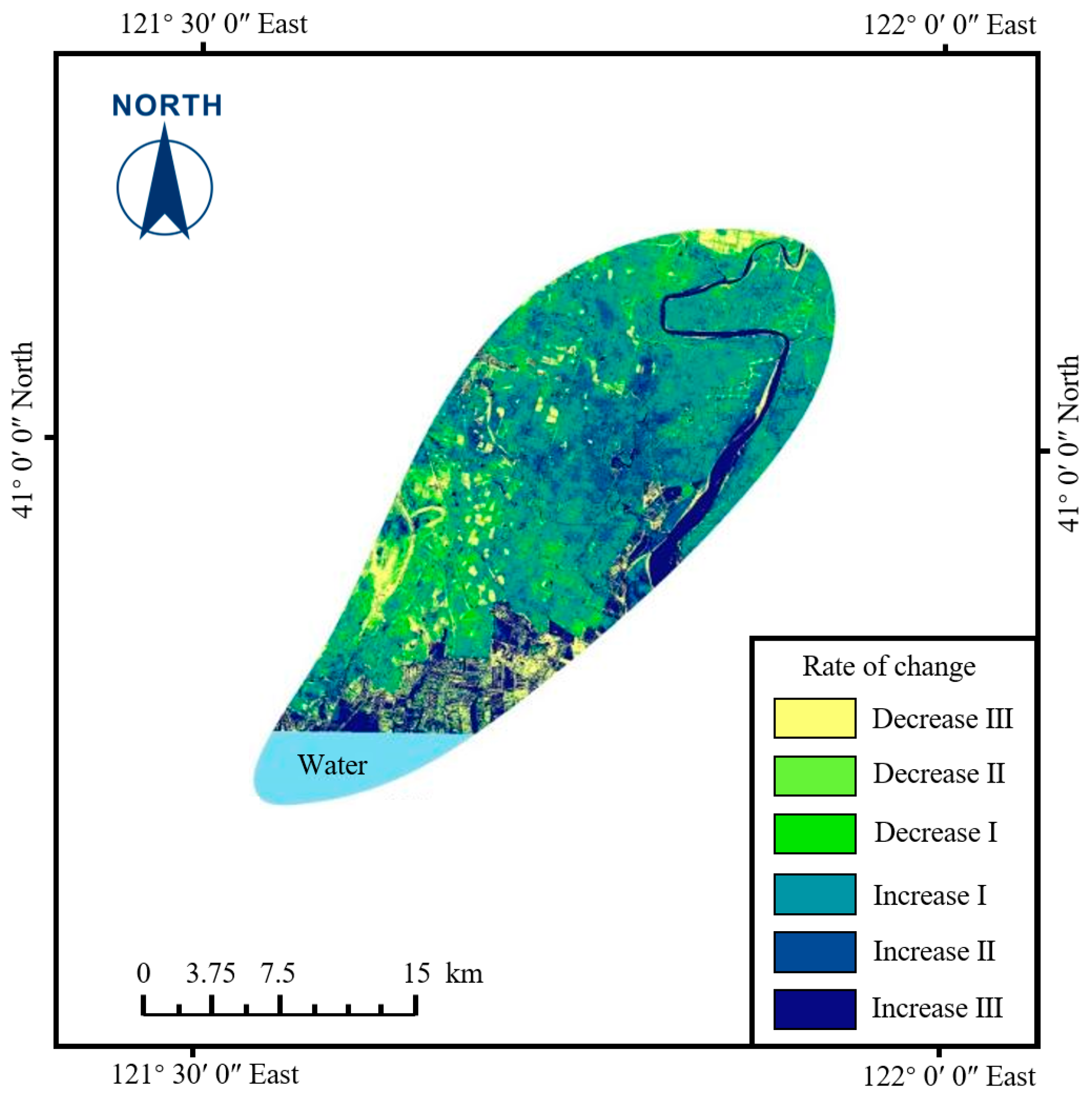
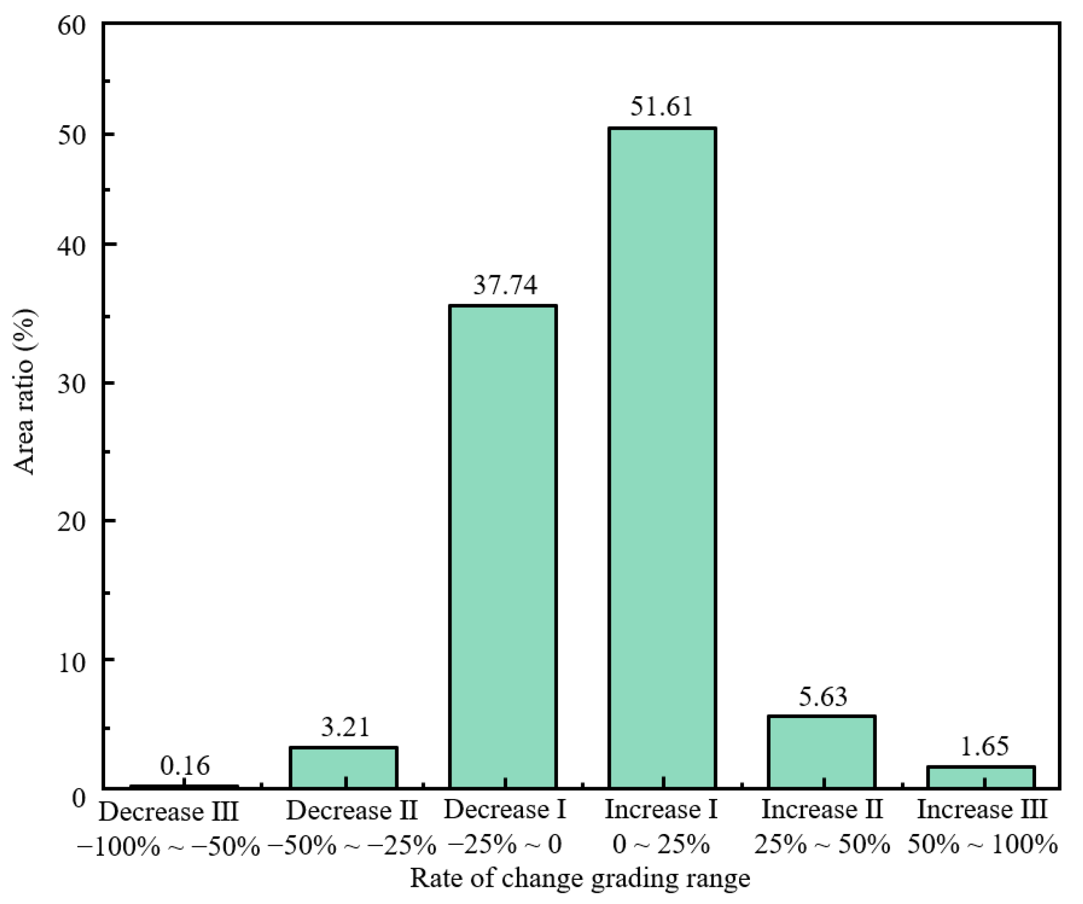
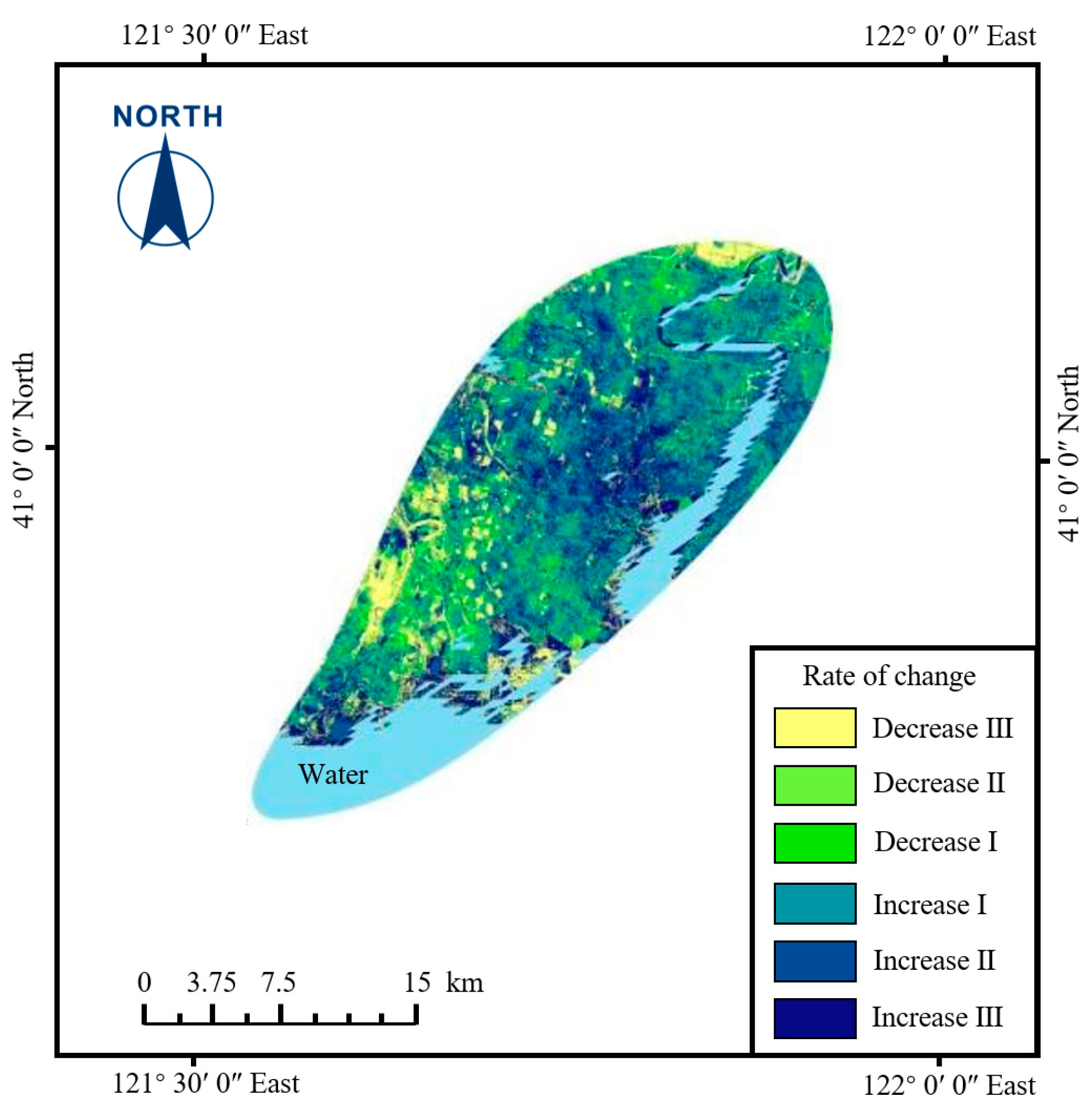
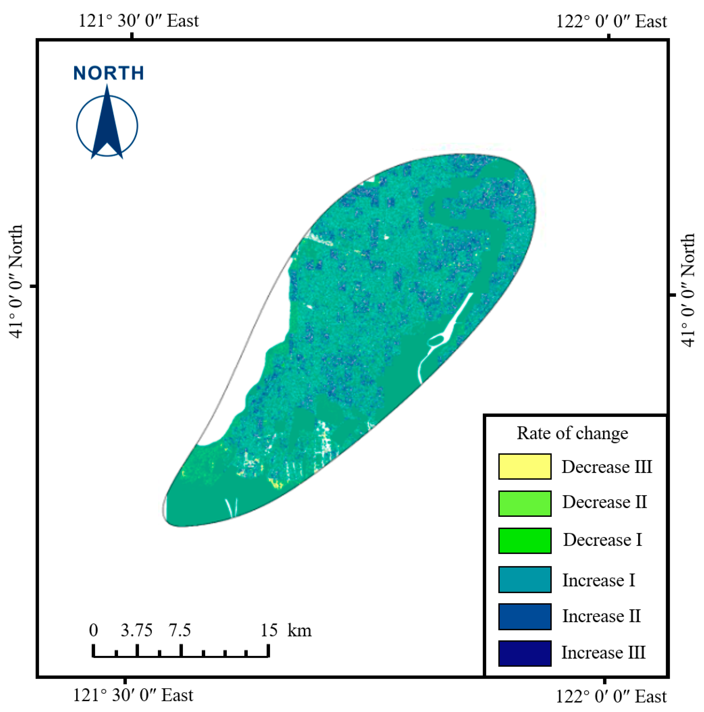
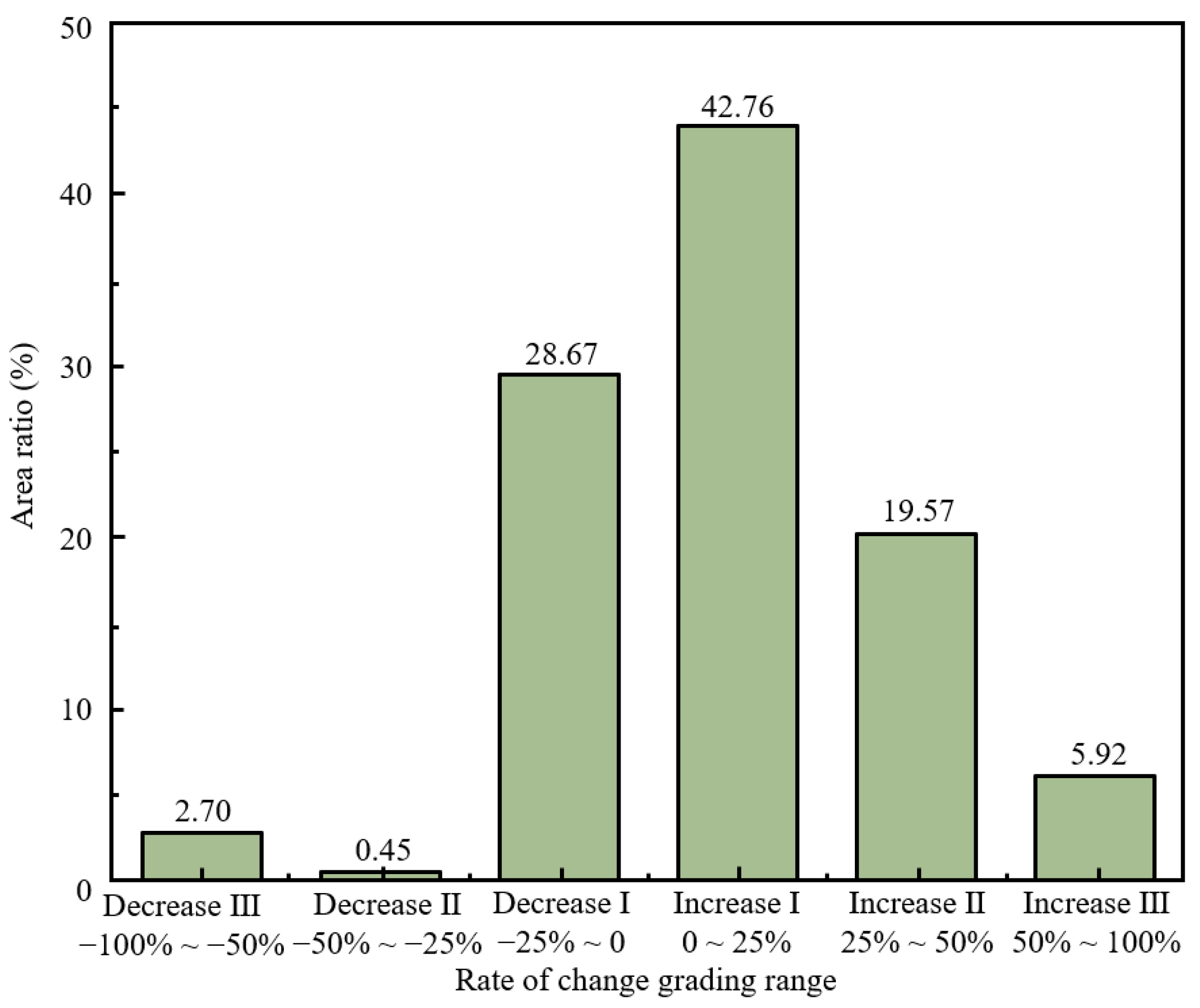
4.2.1. Habitat Quality Index
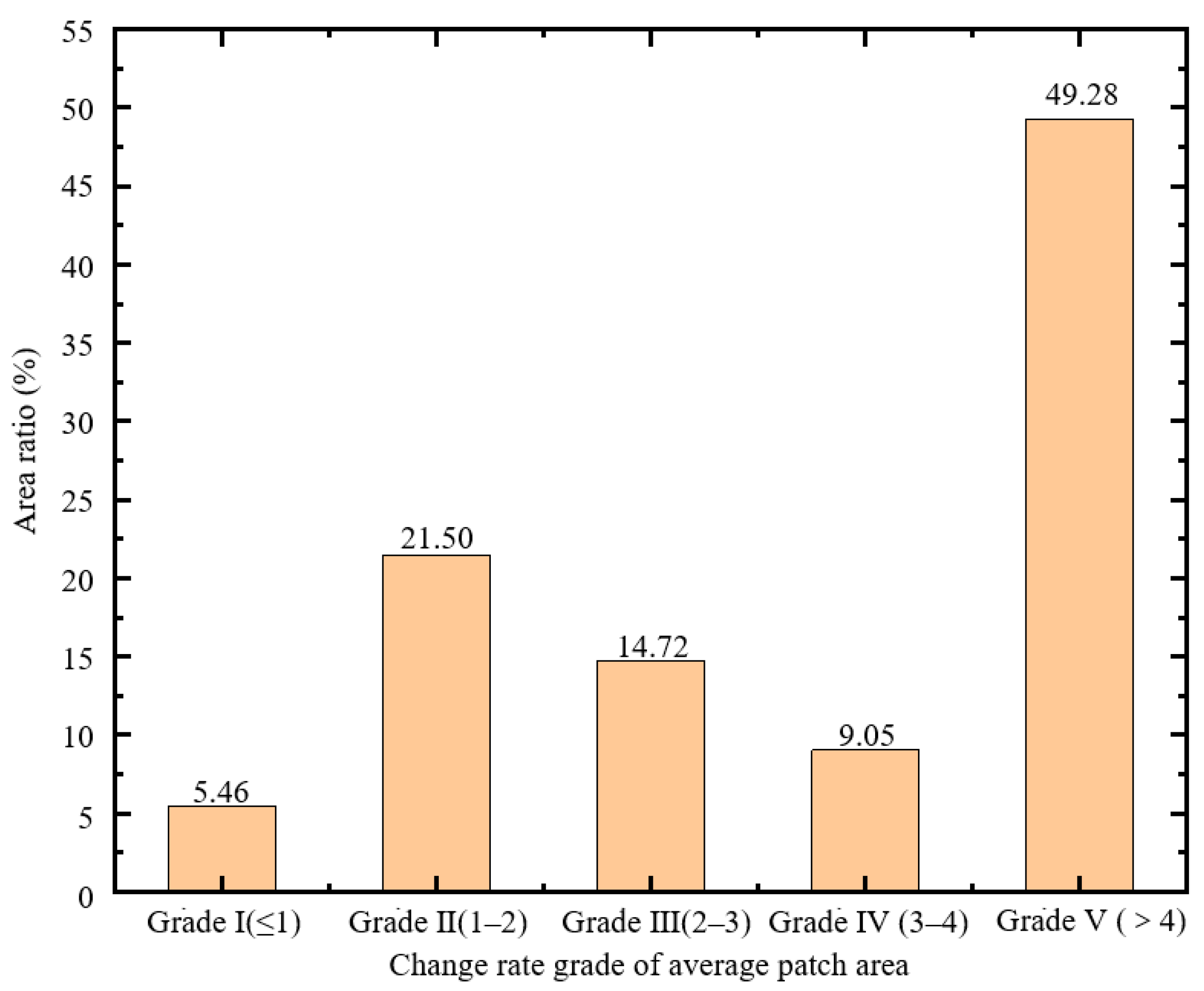
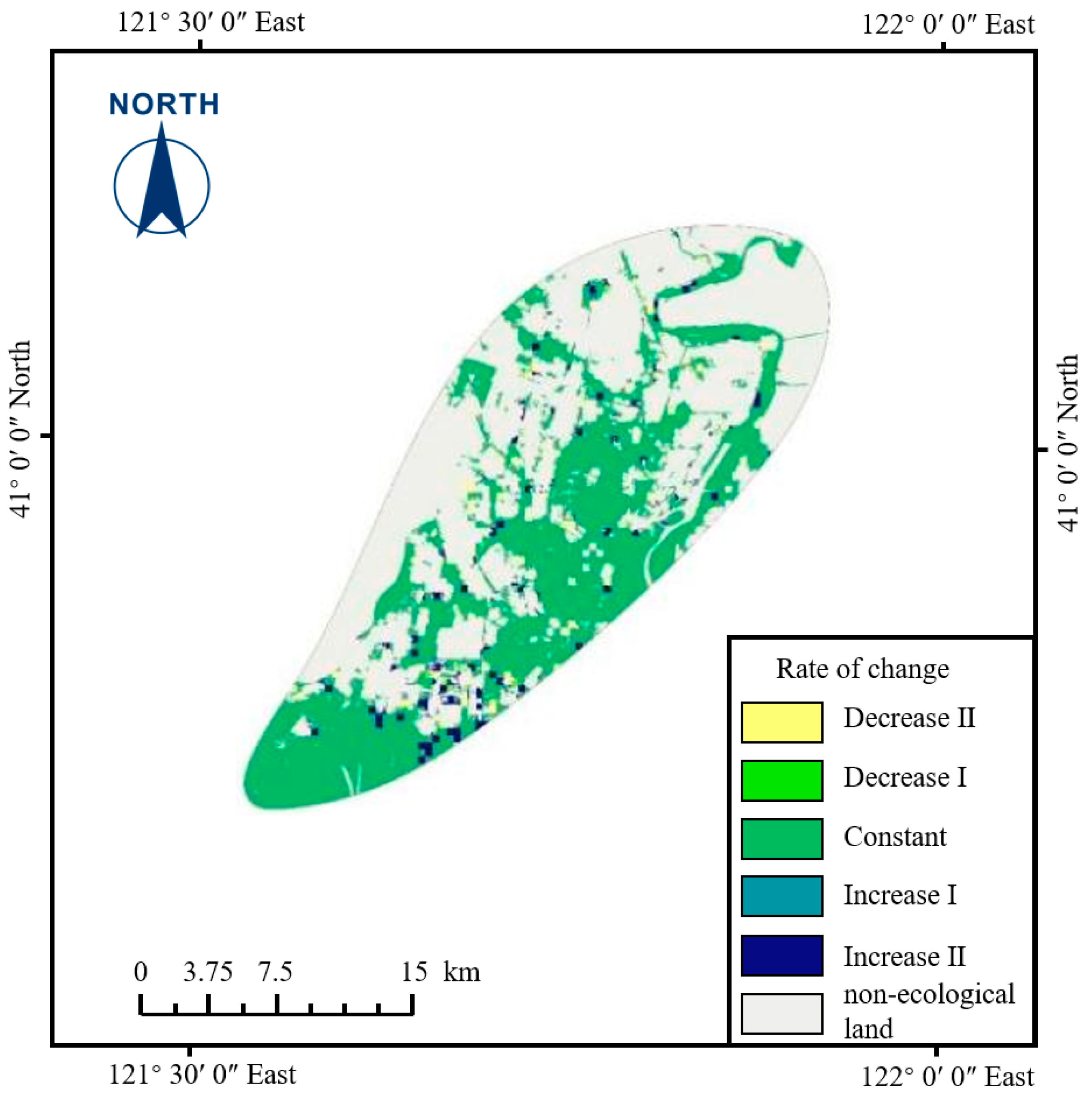
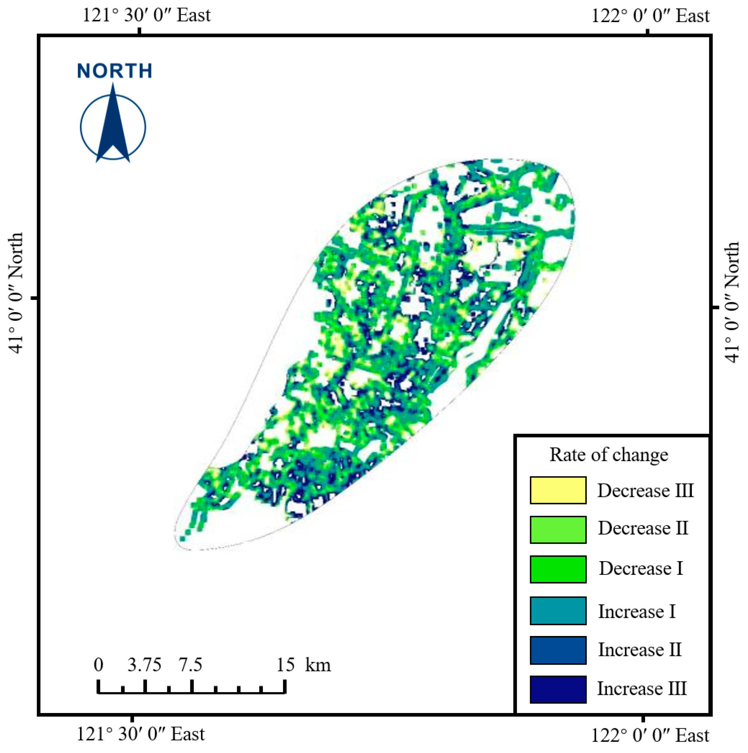
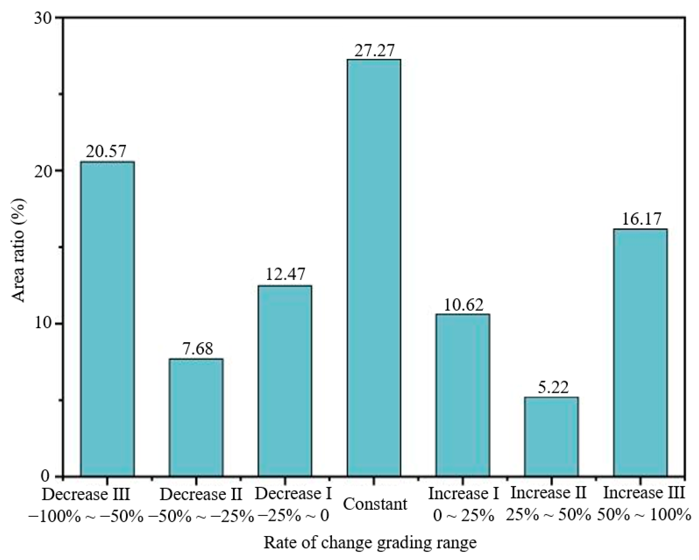
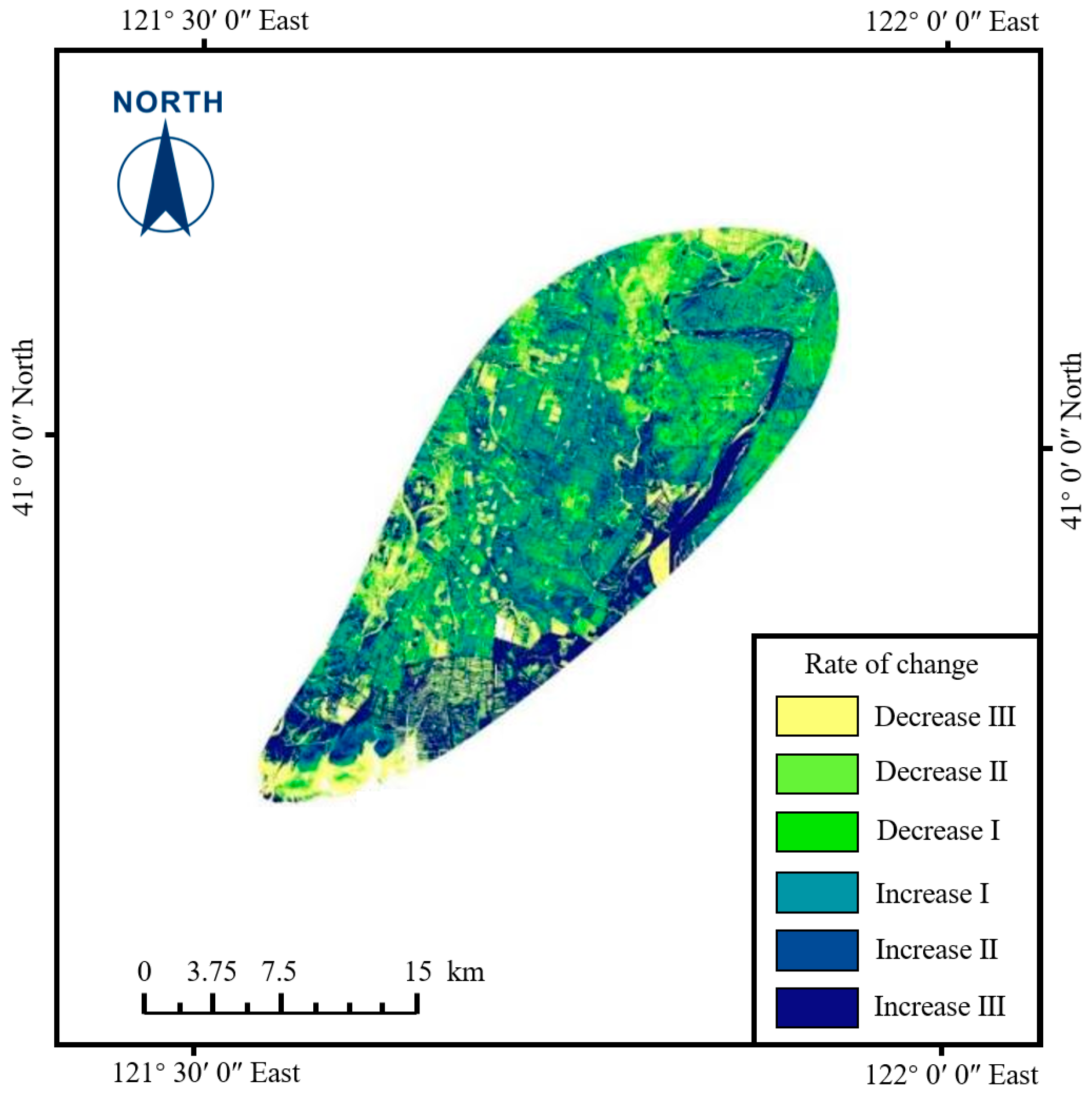
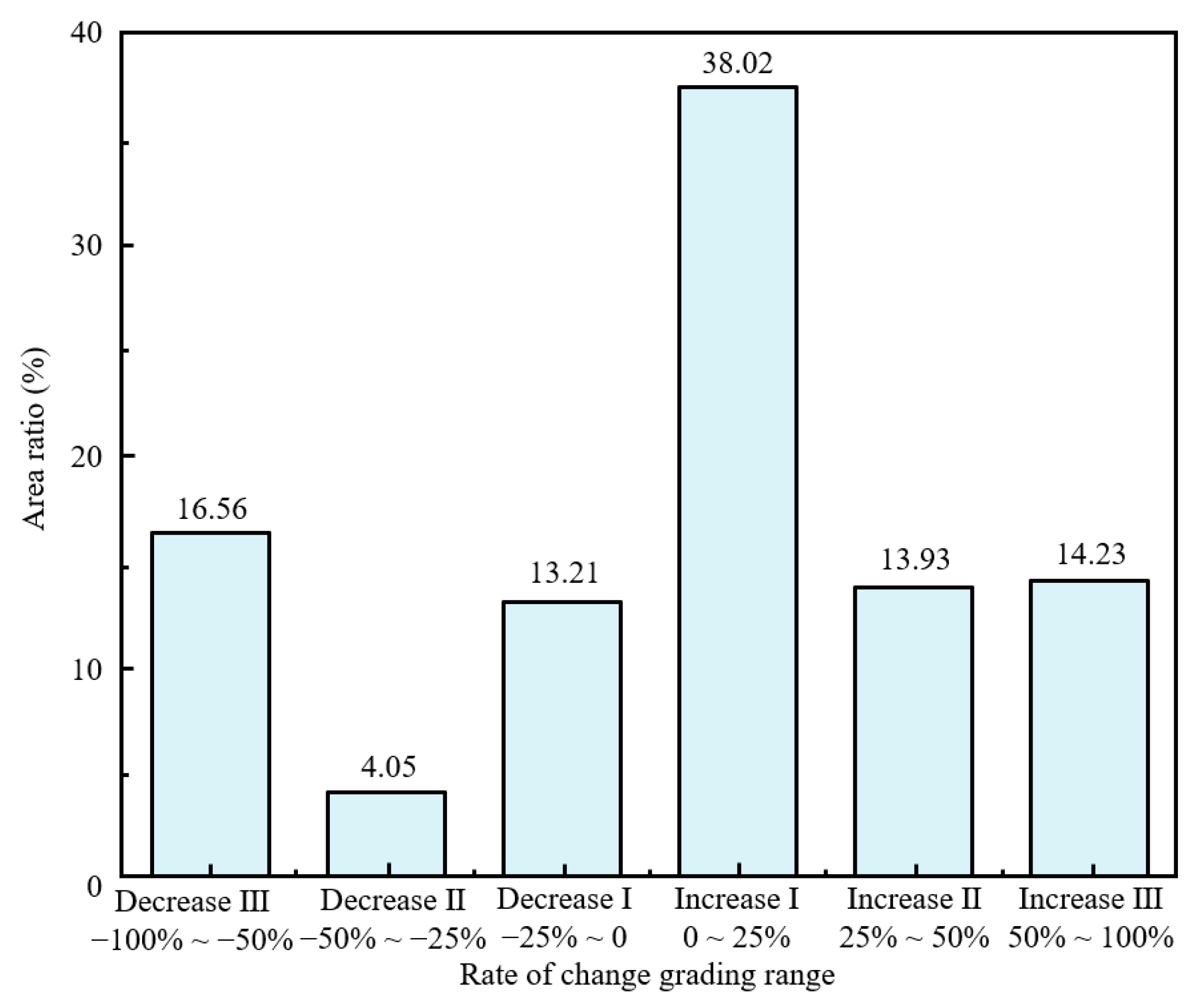
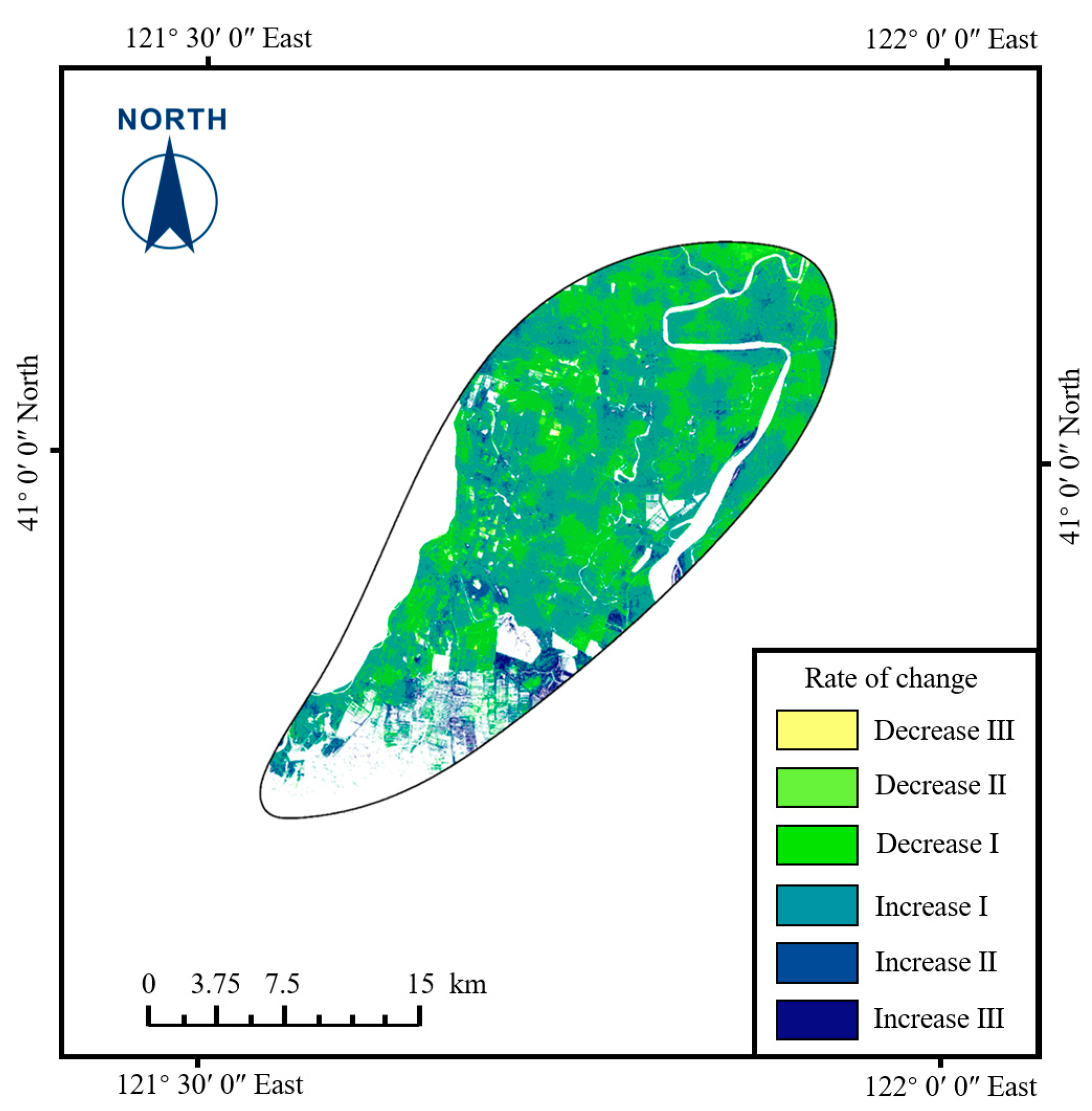
4.2.2. Landscape Fragmentation
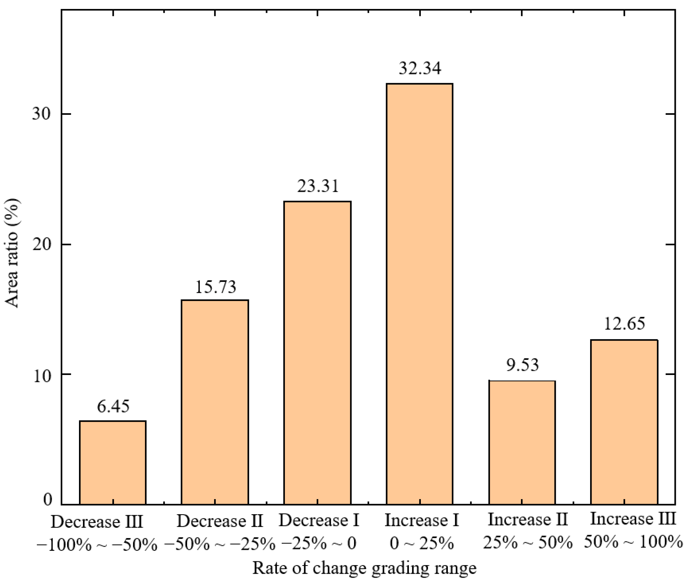
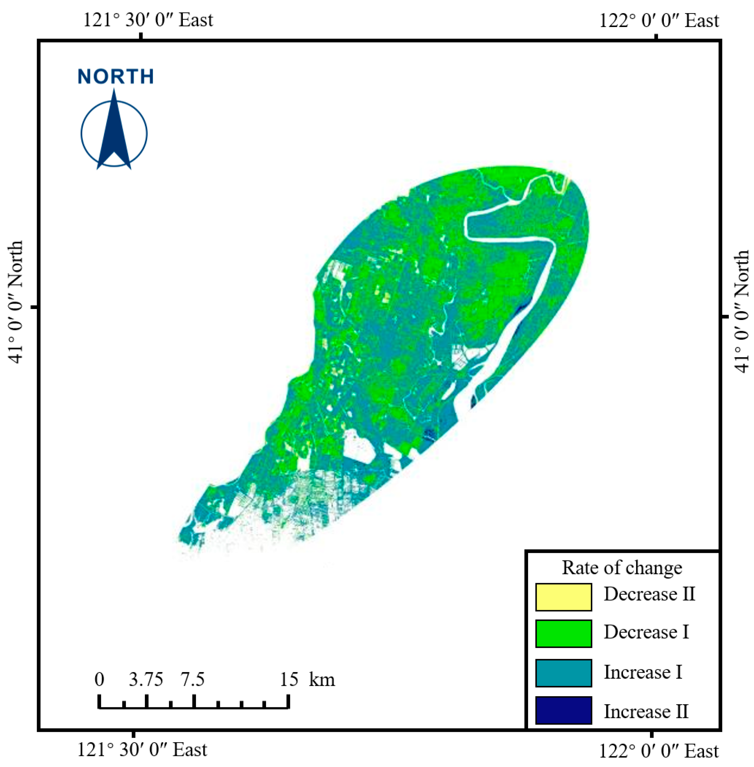
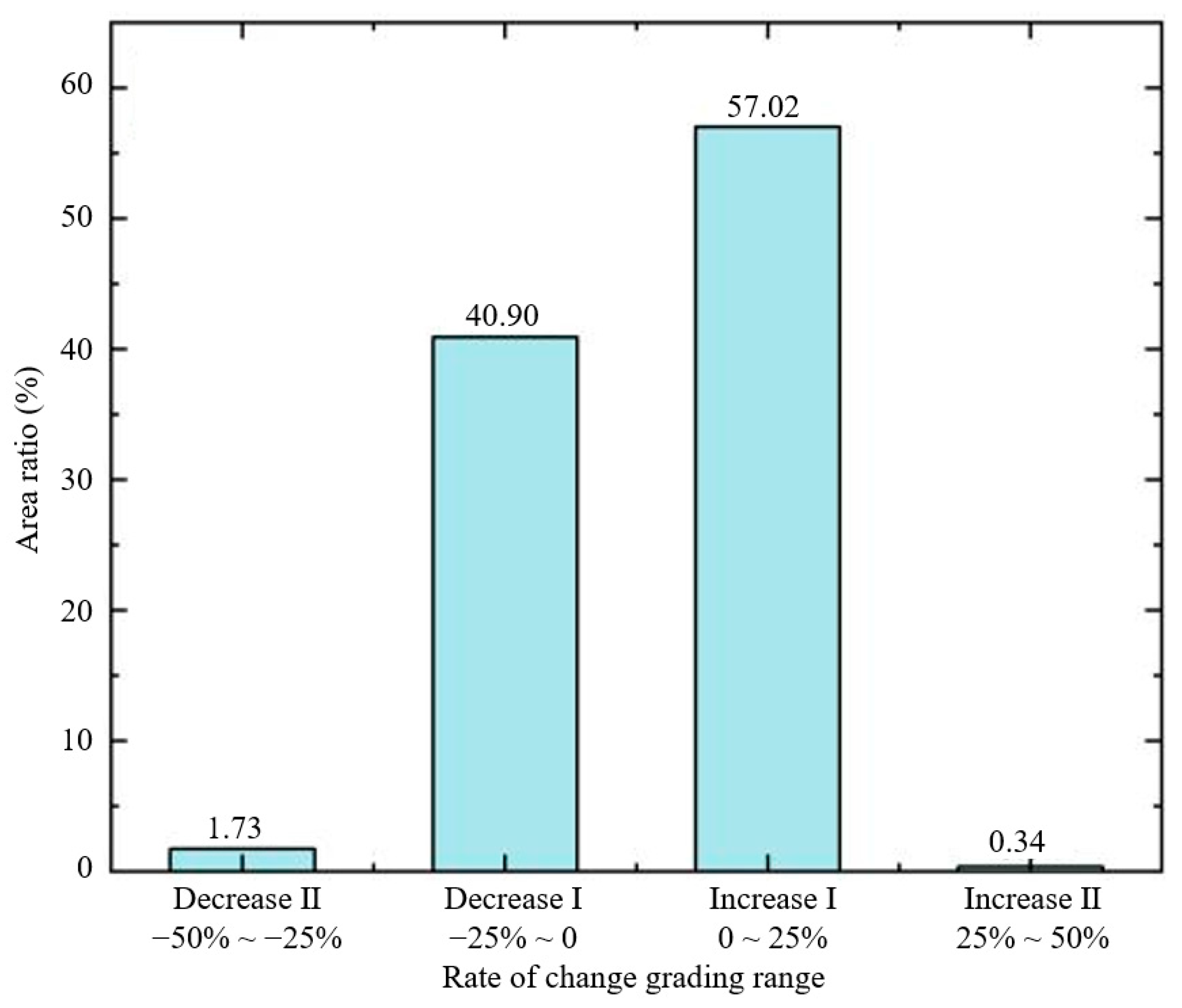
4.2.3. Natural Habitat Connectivity
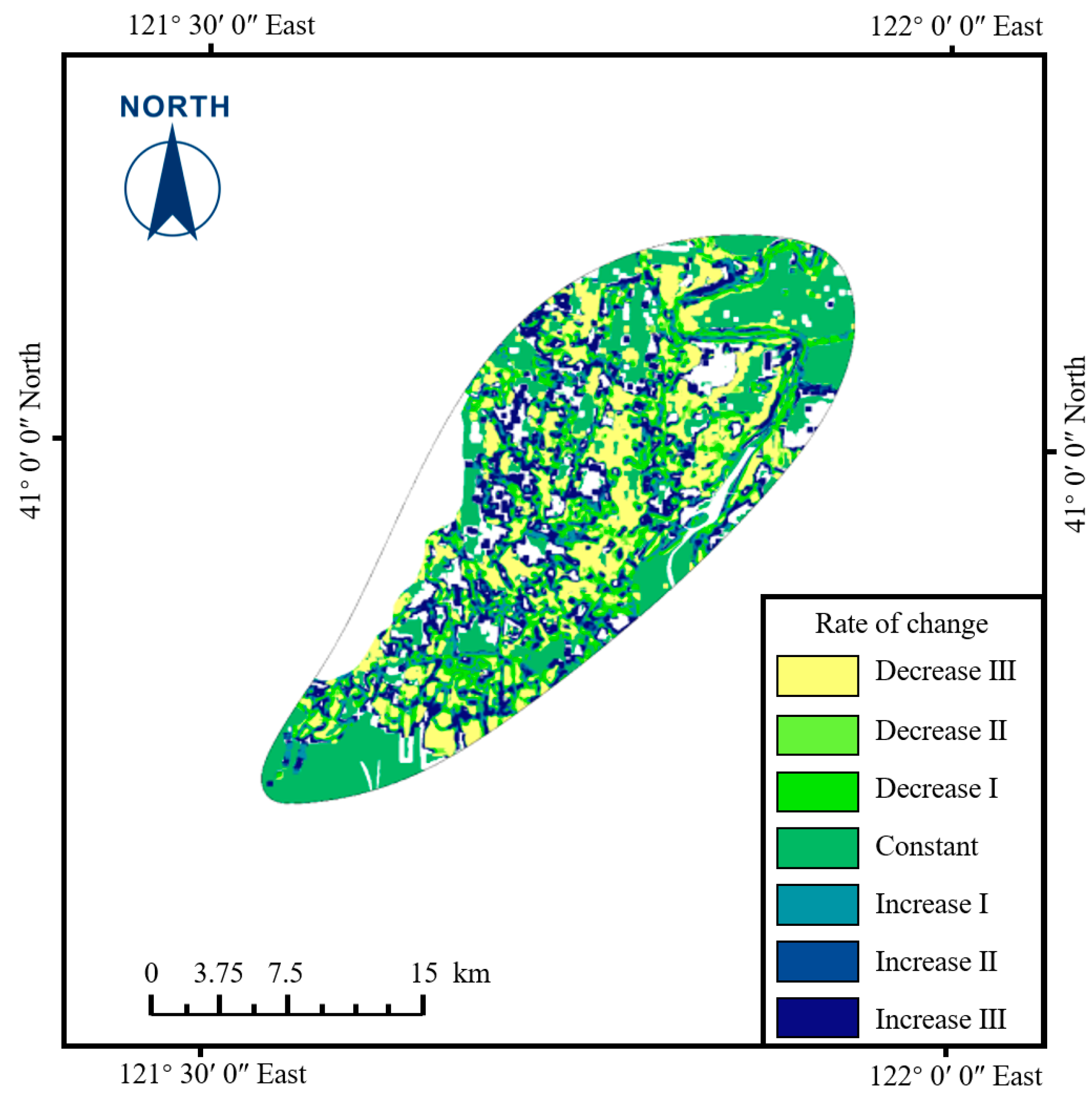
4.2.4. Landscape Stability
4.2.5. Landscape Richness
4.3. Ecosystem Quality Evaluation Results
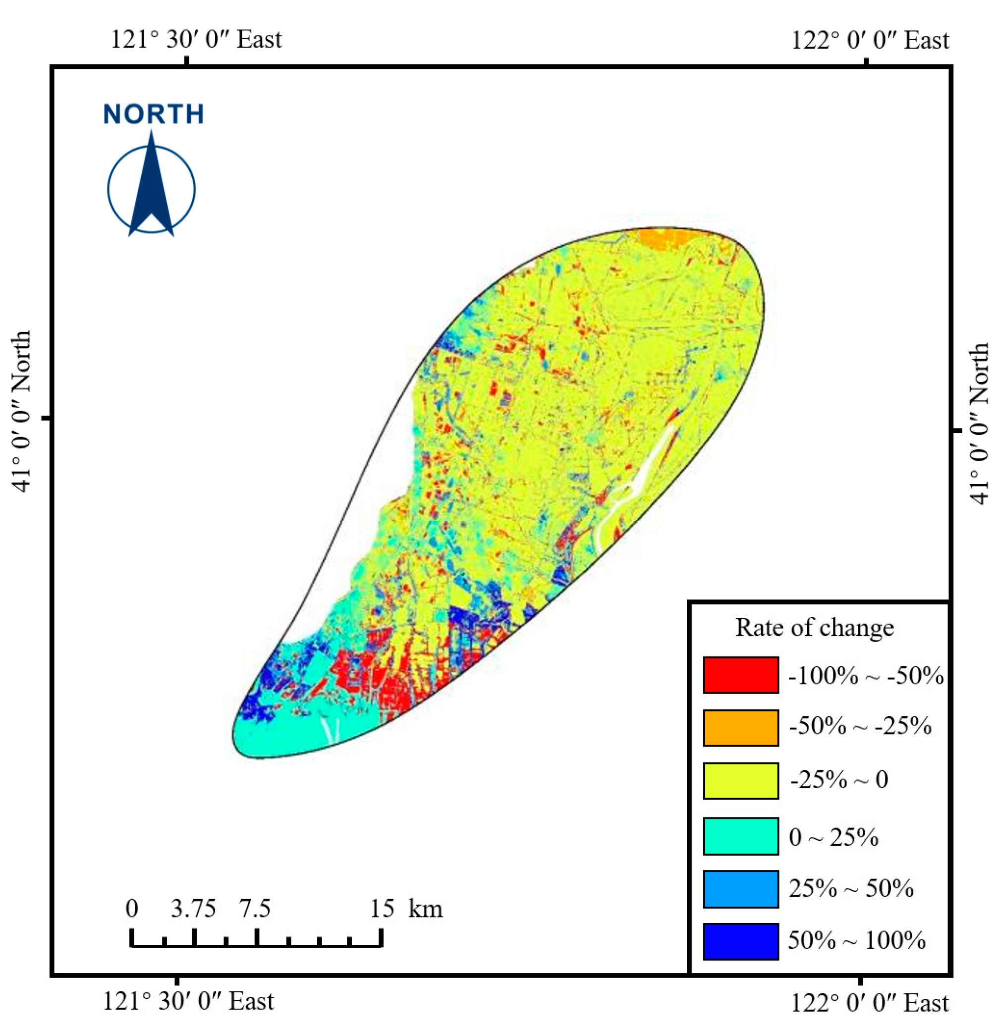
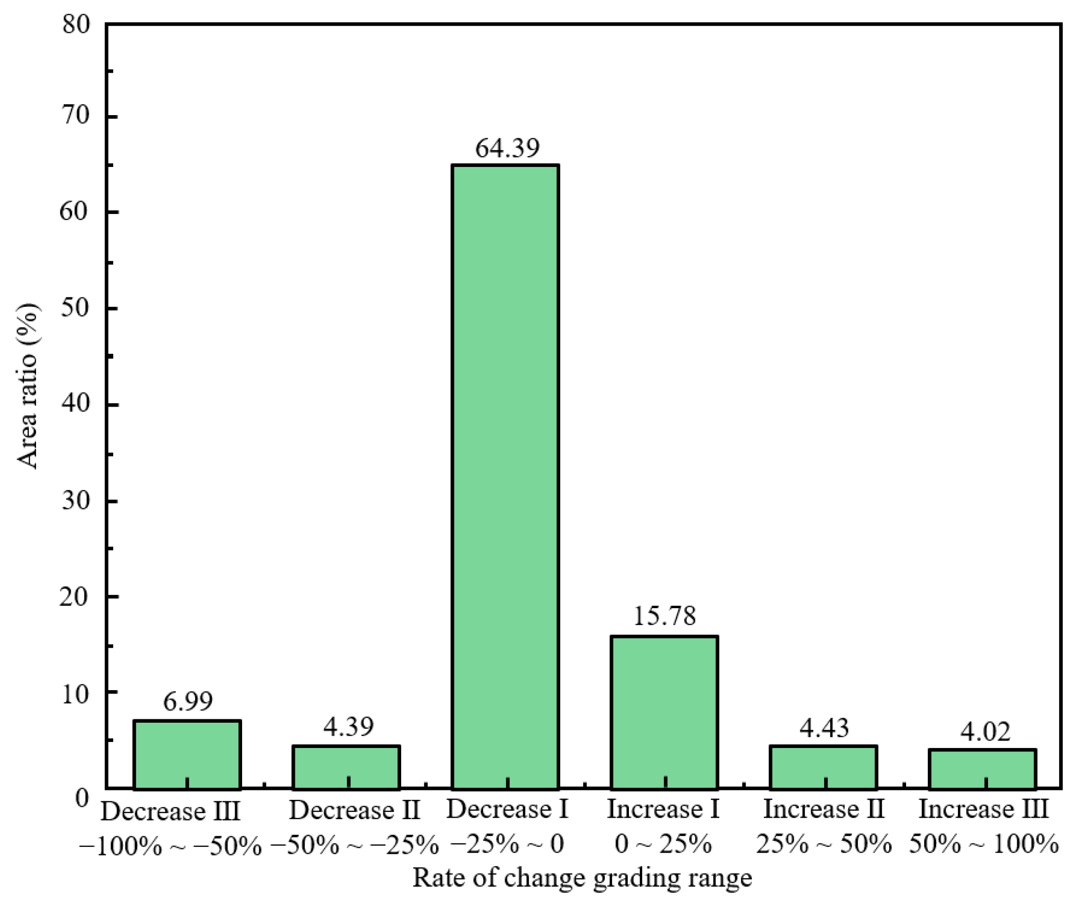
4.3.1. Vegetation Coverage
4.3.2. Leaf Area Index
4.3.3. Gross Primary Productivity
4.4. Ecosystem Service Function Evaluation Results
4.4.1. Biodiversity Conservation
4.4.2. Carbon Sequestration
4.4.3. Water Conservation Capacity
4.4.4. Soil Conservation Amount
5. Discussion
6. Conclusions
Author Contributions
Funding
Institutional Review Board Statement
Informed Consent Statement
Data Availability Statement
Conflicts of Interest
References
- Fu, Z.Y.; Ma, Y.D.; Luo, M.; Lu, Z.H. Research progress on the theory and technology of ecological protection and restoration abroad. Acta Ecol. Sin. 2019, 39, 9008–9021. [Google Scholar]
- Yi, X.; Bai, C.Q.; Liang, L.W.; Zhao, Z.C.; Song, W.X.; Zhang, Y. The evolution and frontier development of land ecological restoration research. J. Nat. Resour. 2020, 35, 37–52. [Google Scholar]
- Barot, S.; Yé, L.; Abbadie, L.; Blouin, M.; Frascaria-Lacoste, N. Ecosystem services must tackle anthropized ecosystems and ecological engineering. Ecol. Eng. 2017, 99, 486–495. [Google Scholar]
- Xiang, H.X.; Wang, Z.M.; Mao, D.H.; Zhang, J.; Xi, Y.B.; Du, B.J.; Zhang, B. What did China’s National Wetland Conservation Program Achieve? Observations of changes in landcover and ecosystem services in the Sanjiang Plain. J. Environ. Manag. 2020, 267, 110623. [Google Scholar]
- Li, L.; Su, F.; Brown, M.T.; Liu, H.; Wang, T. Assessment of ecosystem service value of the liaohe estuarine wetland. Appl. Sci. 2018, 8, 2561. [Google Scholar] [CrossRef]
- Liu, W.W.; Guo, Z.L.; Jiang, B.; Lu, F.; Wang, H.N.; Wang, D.A.; Zhang, M.Y.; Cui, L.J. Improving wetland ecosystem health in China. Ecol. Ind. 2020, 113, 106184. [Google Scholar]
- Lotze, H.K.; Lenihan, H.S.; Bourque, B.J.; Bradbury, R.H.; Cooke, R.G.; Kay, M.C.; Kidwell, S.M.; Kirby, M.X.; Peterson, C.H.; Jackson, J.B.C. Depletion, degradation, and recovery potential of estuaries and coastal seas. Science 2006, 312, 1806–1809. [Google Scholar]
- Wang, Y.Z.; Hong, W.; Wu, C.Z.; He, D.J.; Lin, S.W.; Fan, H.L. Application of landscape ecology to the research on wetlands. J. For. Res. 2008, 19, 164–170. [Google Scholar]
- Bennett, E.M.; Cramer, W.; Begossi, A.; Cundill, G.; Díaz, S.; Egoh, B.N.; Geijzendorffer, I.R.; Krug, C.B.; Lavorel, S.; Lazos, E.; et al. Linking biodiversity, ecosystem services, and human well-being: Three challenges for designing research for sustainability. Curr. Opin. Environ. Sustain. 2015, 14, 76–85. [Google Scholar]
- Li, X.L.; Xue, Z.P.; Gao, J. Dynamic changes of plateau wetlands in Madou County, the Yellow River Source Zone of China: 1990-2013. Wetlands 2016, 36, 299–310. [Google Scholar]
- Kirwan, M.L.; Megonigal, J.P. Tidal wetland stability in the face of human impacts and sea-level rise. Nature 2013, 504, 53–60. [Google Scholar]
- Etienne, F.C.; Benjamin, D.S.; Zhen, Z.; Avni, M.; Joe, R.M.; Benjamin, P.; Jed, O.P. Extensive global wetland loss over the past three centuries. Nature 2023, 614, 281–286. [Google Scholar]
- Davidson, N.C.; Finlayson, C.M. Earth observation for wetland inventory, assessment and monitoring. Aquat. Conserv. 2010, 17, 219–228. [Google Scholar]
- Borja, Á.; Dauer, D.M.; Grémare, A. The importance of setting targets and reference conditions in assessing marine ecosystem quality. Ecol. Indic. 2012, 12, 1–7. [Google Scholar]
- Cheng, X.; Chen, L.D.; Sun, R.H.; Kong, P.R. Land use changes and socio-economic development strongly deteriorate river ecosystem health in one of the largest basins in China. Sci. Total Environ. 2018, 616, 376–385. [Google Scholar]
- Chen, W.; Cao, C.X.; Liu, D.; Tian, R.; Wu, C.Y.; Wang, Y.Q.; Qian, Y.F.; Ma, G.Q.; Bao, D.M. An evaluating system for wetland ecological health: Case study on nineteen major wetlands in Beijing-Tianjin-Hebei region, China. Sci. Total Environ. 2019, 666, 1080–1088. [Google Scholar]
- Su, F.L.; Liu, H.S.; Zhu, D.; Li, L.F.; Wang, T.L. Sustainability assessment of the Liaohe Estuary wetland based on emergy analysis. Ecol. Indic. 2020, 119, 106837. [Google Scholar]
- Sun, T.T.; Lin, W.P.; Chen, G.S.; Guo, P.P.; Zeng, Y. Wetland ecosystem health assessment through integrating remote sensing and inventory data with an assessment model for the Hangzhou Bay, China. Sci. Total Environ. 2016, 566, 627–640. [Google Scholar] [PubMed]
- He, Y.; Hao, J.Y.; He, W.; Lam, K.C.; Xu, F.L. Spatiotemporal variations of aquatic ecosystem health status in Tolo Harbor, Hong Kong from 1986 to 2014. Ecol. Indic. 2019, 100, 20–29. [Google Scholar]
- Cui, Q.; Wang, X.; Li, D.; Guo, X. An ecosystem health assessment method integrating geochemical indicators of soil in Zoige wetland, southwest China. Proc. Environ. Sci. 2012, 13, 1527–1534. [Google Scholar]
- Chi, Y.; Zheng, W.; Shi, H.H.; Sun, J.K.; Fu, Z.Y. Spatial heterogeneity of estuarine wetland ecosystem health influenced by complex natural and anthropogenic factors. Sci. Total Environ. 2018, 634, 1445–1462. [Google Scholar] [PubMed]
- Xu, F.; Yang, Z.F.; Chen, B.; Zhao, Y.W. Ecosystem health assessment of the plant-dominated Baiyangdian Lake based on eco-exergy. Ecol. Model. 2011, 222, 201–209. [Google Scholar]
- Fu, B.L.; Li, Y.; Wang, Y.Q.; Campbell, A.; Zhang, B.; Yin, S.B.; Zhu, H.L.; Xing, Z.F.; Jin, X.M. Evaluation of riparian condition of Songhua River by integration of remote sensing and field measurements. Sci. Rep. 2017, 7, 2565. [Google Scholar]
- Kandissounon, G.A.; Karla, A.; Ahmad, S. Integrating system dynamics and remote sensing to estimate future water usage and average surface runoff in Lagos. Nigeria Civ. Eng. J. 2018, 4, 378. [Google Scholar]
- Tian, H.; Cao, C.; Chen, W.; Bao, S.; Yang, B. Response of vegetation activity dynamic to climatic change and ecological restoration programs in Inner Mongolia from 2000 to 2012. Ecol. Eng. 2015, 82, 276–289. [Google Scholar]
- Del Rio-Mena, T.; Willemen, L.; Tesfamariam, G.T.; Beukes, O.; Nelson, A. Remote sensing for mapping ecosystem services to support evaluation of ecological restoration interventions in an arid landscape. Ecol. Indic. 2020, 113, 106182. [Google Scholar]
- Abbaszadeh Tehrani, N.; Mohd Shafri, H.Z.; Salehi, S.; Chanussot, J.; Janalipour, M. Remotely-Sensed Ecosystem Health Assessment (RSEHA) model for assessing the changes of ecosystem health of Lake Urmia Basin. Int. J. Image Data Fusion 2021, 13, 180–205. [Google Scholar]
- Brannstrom, C. Socioenvironmentalism and new laws: Legal protection of biological and cultural diversity. J. Lat. Am. Stud. 2006, 38, 419–421. [Google Scholar]
- Xia, N.; Tang, Y.Q.; Tang, M.Y.; Quan, W.L.; Xu, Z.J.; Zhang, B.W.; Xiao, Y.X.; Ma, Y.G. Monitoring and evaluation of vegetation restoration in the Ebinur Lake Wetland National Nature Reserve under lockdown protection. Front. Plant Sci. 2024, 15, 1332788. [Google Scholar]
- Gao, S.Q.; Dong, G.T.; Jiang, X.H.; Nie, T.; Yin, H.J.; Guo, X.W. Quantification of natural and anthropogenic driving forces of vegetation changes in the three-river headwater region during 1982–2015 based on geographical detector model. Remote Sens. 2021, 13, 4175. [Google Scholar] [CrossRef]
- Zhang, J.Y.; Ding, J.L.; Wu, P.F.; Tan, J.; Huang, S.; Teng, D.X.; Cao, X.Y.; Wang, J.Z.; Chen, W.Q. Assessing arid inland lake watershed area and vegetation response to multiple temporal scales of drought across the Ebinur lake watershed. Sci. Rep. 2020, 10, 1354. [Google Scholar]
- Chen, Y.H.; Sun, L.; Xu, J.Q.; Liang, B.Y.; Wang, J.; Xiong, N.A. Wetland vegetation changes in response to climate change and human activities on the Tibetan Plateau during 2000–2015. Front. Ecol. Evol. 2023, 11, 1113802. [Google Scholar]
- Wu, X.X.; Lv, M.; Jin, Z.Y.; Michishita, R.; Chen, J.; Tian, H.Y.; Tu, X.B.; Zhao, H.M.; Niu, Z.G.; Chen, X.L.; et al. Normalized difference vegetation index dynamic and spatiotemporal distribution of migratory birds in the Poyang Lake wetland, China. Ecol. Indic. 2014, 47, 219–230. [Google Scholar]
- Shen, Y.L.; Shen, G.L.; Zhai, H.; Yang, C.; Qi, K.L. A Gaussian Kernel-based spatiotemporal fusion model for agricultural remote sensing monitoring. IEEE J. Sel. Top. Appl. Earth Obs. Remote Sensing. 2021, 14, 3533–3545. [Google Scholar]
- Liu, B.; Song, L.Y.; Zhao, Y.W.; Ding, S.M. Research and Application of Space-air-ground Integrated Environmental Monitoring System. Ecol. Environ. Monit. Three Gorges 2023, 8, 17–25. [Google Scholar]
- Chen, Y.P.; Ren, J.; Wang, L. Review on monitoring method of ecological conservation and restoration project area based on multi-source remote sensing data. Acta Ecol. Sin. 2019, 39, 8789–8797. [Google Scholar]
- Li, S.T.; Li, C.Y.; Kang, X.D. Development status and future prospects of multi-source remote sensing image fusion. J. Remote Sens. 2021, 25, 148–166. [Google Scholar]
- Wu, Z.F.; Cao, Z.; Song, S.; Jiang, W.G.; Guo, G.H.; Wu, Y.Y. Wetland remote sensing monitoring and assessment in Guangdong-Hong Kong-Macau Greater Bay Area: Current status, challenges and future perspectives. Acta Ecol. Sin. 2020, 40, 8440–8450. [Google Scholar]
- Luo, M.; Gong, Z.N.; Zhang, Y. Accurate identification of inland wetland dynamic range under water level fluctuation. J. Remote Sens. 2023, 27, 1348–1361. [Google Scholar]
- Duo, A.; Zhao, W.J.; Gong, Z.N.; Zhou, T.G. A Wetland Boundary Information Extraction Method Based on The Inversion of Soil Moisture. J. Henan Norm. Univ. (Nat. Sci.) 2015, 43, 158–163. [Google Scholar]
- Zou, Y.; Li, H.; Zhang, J.B.; Chen, J.Y.; Yang, H.T.; Gong, Z. Inversion of aboveground biomass of saltmarshes in coastal wetland using remote sensing. Acta Ecol. Sin. 2023, 43, 8532–8543. [Google Scholar]
- GB 3838-2002; Environmental Quality Standards for Surface Water. Ministry of Ecology and Environment of the People’s Republic of China: Beijing, China, 2002.
- Cao, C.C.; Su, F.L.; Li, H.F.; Wei, C.; Sun, D. Landscape fragmentation and driving mechanism of Suaeda salsa wetland in Liaohe Estuary. Acta Ecol. Sin. 2022, 42, 581–589. [Google Scholar]
- Guo, M.Y.; Hou, Y.; Huang, C.H.; Zhang, S.Y.; Sun, C.G. Analysis on the Change and Driving Factors of Wetland Landscape in Zhuhai City from 1988 to 2018. Trop. Geomorphol. 2020, 41, 1–7. [Google Scholar]
- Zhao, R.F.; Jiang, P.H.; Zhao, H.L.; Fan, J.P. Fragmentation process of wetlands landscape in the middle reaches of the Heihe River and its driving forces analysis. Acta Ecol. Sin. 2013, 33, 4436–4449. [Google Scholar]
- Yang, Y.Q.; Gong, A.D.; Zhang, Y.H.; Chen, Y.L. Dynamic changes in Zhalong Wetland landscape from 1980 to 2015. J. Beijing Norm. Univ. (Nat. Sci.) 2021, 57, 624–630. [Google Scholar]
- Yang, C.; Chen, Y.J. Research progress and prospects of avian studies in the Zoige Wetland. Chin. J. Appl. Environ. Biol. 2024, 30, 841–847. [Google Scholar]
- Wu, T.T.; Ding, S.; Chen, Z.Z.; Lei, J.R.; Chen, X.H.; Li, Y.L. Dynamic Analysis of Mangrove Wetlands Based on LUCC and Landscape Pattern Change in Dongzhai Port. For. Res. 2020, 33, 154–162. [Google Scholar]
- Wang, D.; Zhu, R.; Zhang, X.; Huang, Z.; Li, C.; Zhang, X. Monitoring and Effect Evaluation of an Ecological Restoration Project Using Multi-Source Remote Sensing: A Case Study of Wuliangsuhai Watershed in China. Land 2023, 12, 349. [Google Scholar] [CrossRef]
- Ma, Z.Q.; Wang, H.M.; Yang, F.T.; Fu, X.L.; Fang, H.J.; Wang, J.S.; Dai, X.Q.; Kou, L.; Zhao, B. Ecological Restoration and Sustainable Development of Forest Ecosystem in Subtropical Red Soil Hilly Region Based on Long-term Observation and Research. Bull. Chin. Acad. Sci. 2020, 35, 1525–1536. [Google Scholar]
- Li, Q.S.; Liu, J.Q.; Li, J.; Zhang, C.Y.; Guo, J.T.; Wang, X.J.; Ran, W.Y. Digital twin of mine ecological environment: Connotation, framework and key technologies. J. Chin. Soc. Coal Sci. 2023, 48, 3859–3873. [Google Scholar]


| Data Type | Data Source | Remote Sensing Monitoring Index for Ecological Restoration Units |
|---|---|---|
| Sentinel-2 land use/land cover | ESRI | Landscape stability (spread, patch density, total edge contrast), habitat quality index, habitat connectivity index, landscape richness, landscape fragmentation, habitat irreplaceability index, water cultivation, net primary productivity, autotrophic respiration, total primary productivity |
| Sentinel-2 reflectance data | European Space Agency (ESA) | Leaf area index, biodiversity index, vegetation cover, water retention, soil conservation |
| Species distribution data | GBIF | Habitat irreplaceability index |
| Temperature data | ERA5-Land | Gross primary productivity, net primary productivity, autotrophic respiration |
| Rainfall data | ERA5-Land | Water conservation, soil conservation, net primary productivity, autotrophic respiration |
| Soil data | HWSD v1.2 | Soil conservation, gross primary productivity, net primary productivity, autotrophic respiration |
| DEM elevation data | SRTM1 | Soil conservation |
| Level | Excellent | Good | Medium | Low | Poor |
|---|---|---|---|---|---|
| Ecosystem Quality | EQI ≥ 75 | 55 ≤ EQI < 75 | 35 ≤ EQI < 55 | 20 ≤ EQI < 35 | EQI < 20 |
Disclaimer/Publisher’s Note: The statements, opinions and data contained in all publications are solely those of the individual author(s) and contributor(s) and not of MDPI and/or the editor(s). MDPI and/or the editor(s) disclaim responsibility for any injury to people or property resulting from any ideas, methods, instructions or products referred to in the content. |
© 2025 by the authors. Licensee MDPI, Basel, Switzerland. This article is an open access article distributed under the terms and conditions of the Creative Commons Attribution (CC BY) license (https://creativecommons.org/licenses/by/4.0/).
Share and Cite
Hou, Y.; Hu, N.; Teng, C.; Zheng, L.; Zhang, J.; Gong, Y. Monitoring and Evaluation of Ecological Restoration Effectiveness: A Case Study of the Liaohe River Estuary Wetland. Sustainability 2025, 17, 2973. https://doi.org/10.3390/su17072973
Hou Y, Hu N, Teng C, Zheng L, Zhang J, Gong Y. Monitoring and Evaluation of Ecological Restoration Effectiveness: A Case Study of the Liaohe River Estuary Wetland. Sustainability. 2025; 17(7):2973. https://doi.org/10.3390/su17072973
Chicago/Turabian StyleHou, Yongli, Nanxiang Hu, Chao Teng, Lulin Zheng, Jiabing Zhang, and Yifei Gong. 2025. "Monitoring and Evaluation of Ecological Restoration Effectiveness: A Case Study of the Liaohe River Estuary Wetland" Sustainability 17, no. 7: 2973. https://doi.org/10.3390/su17072973
APA StyleHou, Y., Hu, N., Teng, C., Zheng, L., Zhang, J., & Gong, Y. (2025). Monitoring and Evaluation of Ecological Restoration Effectiveness: A Case Study of the Liaohe River Estuary Wetland. Sustainability, 17(7), 2973. https://doi.org/10.3390/su17072973