Abstract
This study investigates the carbon- and cost-effectiveness of decarbonization strategies in retrofits of prototypical single-family homes built before 1980 in Houston, Los Angeles, and Chicago, USA. When investigating the carbon performance of home retrofits, embodied carbon, location-specific electricity grid emission rates, variation in future grid emission rates depending on policy changes, and the time value of carbon (TVC) are often omitted. If those subjects are addressed, they are rarely analyzed all together. Using energy simulation and Life Cycle Assessment, this research quantified the whole-life carbon reduction and Life Cycle Cost, in kgCO2e/US$, associated with each retrofit, ranked the interventions accordingly, and calculated how the rankings would change if electricity grid emission rates differed or the TVC were considered. Assuming current grid emission rates, envelope retrofits tended to rank better than renewable energy and electrification upgrades in terms of carbon reduction per dollar spent. However, if grid emission rates were lower, electrification upgrades improved in rank, while renewable energy upgrades declined. Including the TVC generally caused retrofits with high initial carbon to drop in rank. The results illustrate that considering whole-life carbon, regionally specific grid emissions, future grid emission scenarios, and the TVC can have important implications on decarbonization recommendations, and the findings suggest that analyses, especially those supporting building policy or incentive programs, should include such considerations.
1. Introduction
Single-family homes represent 54.4% of floor area in the US existing building stock [1,2,3], making residential retrofits in countries like the US crucial in decarbonizing the built environment. Key emissions-reduction strategies include (1) electrifying buildings, which involves replacing fossil-fuel based systems and appliances with systems that run on electric power, (2) upgrading building envelopes, and (3) adding renewable energy generation. These strategies have gained substantial support in recent years [4,5]. Meanwhile, renewable energy has become the least expensive power source, and solar energy has rapidly scaled up in response [6].
Past studies ranking different building retrofits have focused on energy and cost reductions using source energy normalized by area [7,8,9]. While the source energy metric should capture the effect of different electric grids’ fuel mixes, many practitioners and energy modeling software, including EnergyPlus and DesignBuilder [10,11], rely on national averages by default to convert from site to source energy. As a result, many source energy values are not fine-grained enough to capture utility-specific variations in energy consumption.
Recent retrofit optimization studies incorporate greenhouse gas (GHG) emissions alongside source energy results [12,13,14]. However, they often overlook the embodied carbon of building materials, which becomes more significant as buildings become more efficient [5,15]. One study found that embodied emissions constitute approximately 20% of life cycle GHG emissions on average, rising to 45% in high-efficiency buildings and 90% in extreme cases, suggesting the growing importance of accounting for embodied carbon when considering environmental impacts of buildings [16]. Most studies that evaluate embodied carbon do not consider how the optimal retrofit package would change with a different grid carbon emission intensity. While [17] examines retrofit envelope upgrades under different grid scenarios, research tracking multiple decarbonization strategies over time remains limited.
Furthermore, carbon reductions today are worth more than the same carbon decrease in the future [18]. The U.S. Environmental Protection Agency (EPA) has used this concept to develop the Social Cost of Carbon (SCC), which is a cost estimate of the economic damages that would result from emitting one additional ton of greenhouse gases [19]. This study borrows from the EPA’s methodology to demonstrate how considering the time value of carbon (TVC) can impact the prioritization of building efficiency upgrades.
Building on [20], this study fills a critical gap in the existing literature by including analysis of embodied carbon, electricity grid decarbonization, future grid decarbonization scenarios, and the time value of carbon (TVC), all of which are commonly omitted from studies on building performance upgrades and rarely assessed together. More importantly, including these factors has a significant impact on which retrofits save the greatest carbon at the lowest price, suggesting that expanding the scope of carbon calculations has important implications for decarbonization recommendations.
Project Scope
This study evaluates the carbon- and cost-effectiveness of three decarbonization strategies for residential retrofits: building electrification, envelope upgrades, and on-site renewable energy generation. In this study, building electrification entails installing new electricity-fueled systems for cooking, water heating, and space heating in place of existing gas-fueled systems, as described in Section 2.2.2 and Section 2.3.3. Envelope upgrades include improvements to the home’s wall insulation, ceiling insulation, air tightness, and windows, as described in Section 2.2.3, Section 2.2.4 and Section 2.3.4. Lastly, the addition of on-site renewable energy is limited to roof-mounted photovoltaic (PV) systems, as described in Section 2.2.5 and Section 2.3.5. All proposed retrofit interventions are introduced in 2020, and the carbon and cost expenditures through 2050 are included in the scope.
The study focuses on pre-1980s detached, single-family homes that have not undergone significant energy upgrades. These older homes tend to use more energy than newer homes in part because they were constructed before energy codes began requiring more energy-efficient building practices [21]. Pre-1980s single-family homes currently make up about 64.5% of the residential building stock [1]. The authors evaluated prototypical homes in Houston, Texas (TX) (ASHRAE climate zone 2A, Köppen Classification Cfa) to represent a city with a mid-range electricity grid emission rate, Los Angeles, California (CA) (ASHRAE climate zone 3B, Köppen Classification BSh, Csa and Csb) to represent a city with a low electricity grid emission rate, and Chicago, Illinois (IL) (ASHRAE climate zone 5A, Köppen Classification Dfa) to represent a city with a high grid emission rate.
2. Materials and Methods
2.1. Translating the Prototype Model to the Base Case Model
2.1.1. Prototype Building Assumptions
This study used the single-family residential prototype models developed by the U.S. Department of Energy (DOE), as part of the Building Energy Codes Program, for baseline assumptions [22]. The models’ energy-related specifications are based on the 2006 International Energy Conservation Code (IECC), and all simulations were run in EnergyPlus (EP) version 9.5, a widely validated DOE tool [23]. The base case homes are assumed to have a slab foundation and gas furnace for heating based on the most common systems by census division across all three selected cities [24]. All prototypes share the same building dimensions, window placements, occupancy, schedules, and equipment, as shown in Figure 1.
Figure 1.
Residential prototype model characteristics common to all single-family residential EP prototype models.
The prototype models were designed to establish a minimum level of building performance for building code development, but this study aims to estimate the energy performance of typical existing homes. The base case model represents a typical pre-1980s home, adapted from the 2006 prototype energy models, as described in Section 2.1.3.
2.1.2. Energy Model Calibration Between EnergyPlus and DesignBuilder
To develop the base case model, the 2006 prototype model developed in EP was translated into a comparable 2006 model in DesignBuilder version 7.0.0.116. Most parameters were directly transferred from the EP Input Data File (IDF) file into the DesignBuilder model settings. For the inputs that required translation from EP to DesignBuilder, the methods are described in Section S2 of the Supplementary Materials. After verifying minimal differences in energy consumption between the models (the results are provided in Table S5 of the Supplementary Materials), the pre-1980s base case model was developed in DesignBuilder.
2.1.3. Base Case Development
The base case model represents a typical pre-1980s home, while the calibrated DesignBuilder model was initially based on a 2006 home. The simulation parameters were updated to reflect pre-1980s characteristics (Table 1, Table 2 and Table 3). The features not found in older homes, such as mechanical ventilation, under-slab insulation, or vertical insulation at the slab perimeter, were removed. The base case assumes uninsulated walls and minimal attic insulation.
Table 1.
Houston electrification retrofit interventions and energy model performance targets.
Table 2.
Houston envelope retrofit interventions and energy model performance targets.
Table 3.
Houston renewable energy retrofit interventions and energy model performance targets.
Infiltration rates were based on a study that reviewed air exchange rates in existing residential buildings in Detroit, Michigan; Elizabeth, New Jersey; Houston, Texas; and Los Angeles, California [25]. Infiltration values from Houston and Los Angeles were used for the corresponding cities. For Chicago homes, infiltration values from Detroit (which shares the same climate zone as Chicago) were used. All cities used the 50th percentile air exchange rates, with Houston’s rates detailed in Table 2.
Operable windows were assumed to have a 50% openable area, with natural ventilation settings allowing occupant control when beneficial. The base case homes include gas appliances for cooking, water heating, and space heating.
2.2. Operational Energy
2.2.1. Overview: Estimating Operational Energy Reductions
The study used DesignBuilder to quantify the operational energy savings from each retrofit intervention [26]. Table 1, Table 2 and Table 3 summarize the base case and retrofit assumptions in Houston, while details for Los Angeles and Chicago are in the Supplementary Materials. Each retrofit intervention was applied one at a time to the base case energy model. The difference in energy consumption between the base case and energy retrofit model equals the energy savings associated with the intervention. Assumptions and target performance values varied slightly by city to reflect climate differences.
2.2.2. Electrification Retrofit, Operational Energy Assumptions
The electrification decarbonization scenario included three separate retrofit interventions: replacing the gas stove, water heater, and space heating with higher-performing electric alternatives. A combined “electrification all” scenario simulated all three swaps together. In the energy simulations, the authors used the equipment specifications for the electric stove, heat pump water heater, and air-source heat pump found in the DOE electrified prototype models per Table 1. Modeling of the air-source heat pump was simplified using evidence from the past literature, as described in Section S4.4 of the Supplementary Materials.
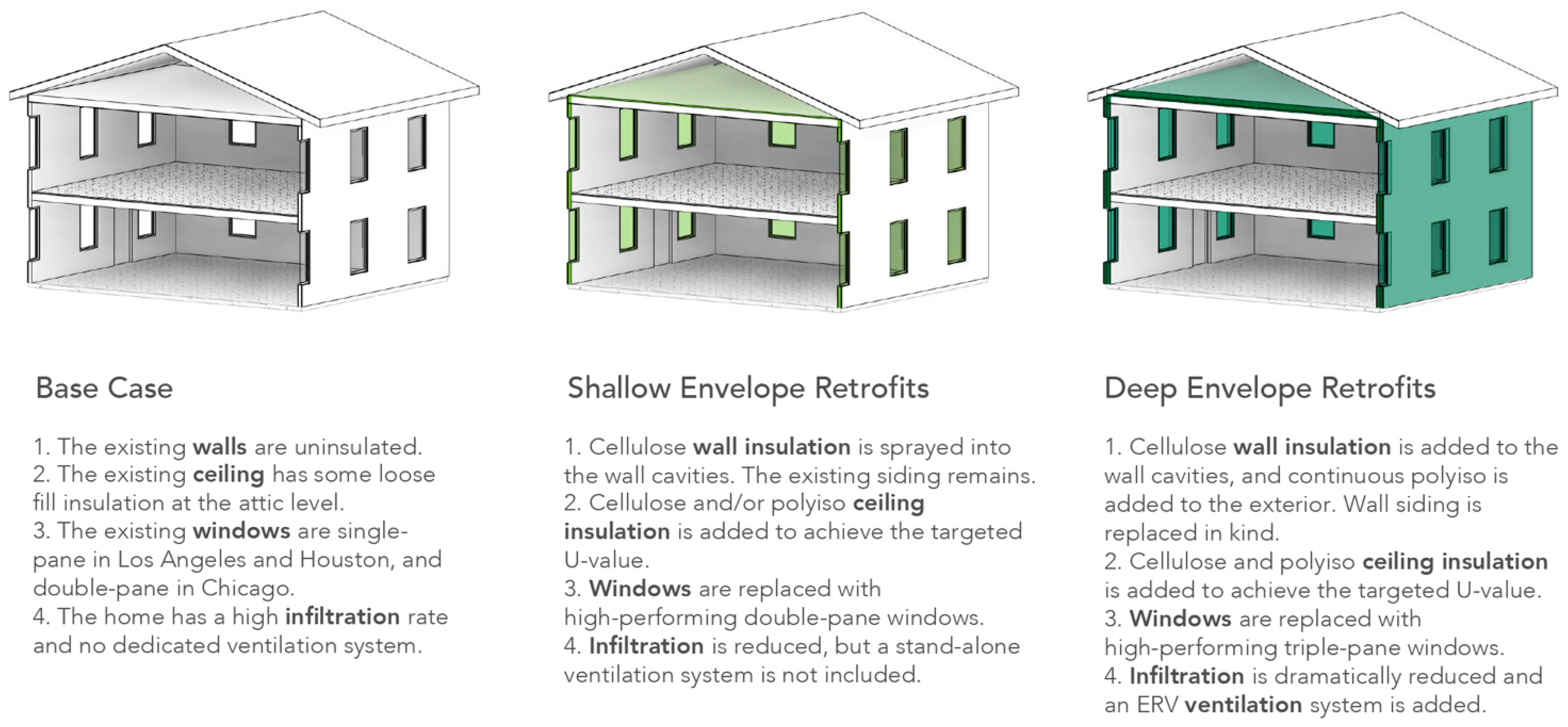
2.2.3. Shallow Envelope Retrofit, Operational Energy Assumptions
The shallow envelope upgrade scenarios included improved ceiling insulation, wall insulation, windows, and infiltration, each applied individually. The authors also combined these measures into one intervention, called “shallow all”. The “shallow envelope” intervention combined ceiling insulation, wall insulation, and infiltration upgrades (but not window upgrades). The target values for each intervention are outlined in Table 2.
The 2021 International Residential Code (IRC) was used to set the infiltration rate and window specifications for shallow retrofits. The 5ACH50 infiltration target is achievable with standard air sealing, and the IRC had the least restrictive window specifications of the standards reviewed [27,28]. Window glazing specifications followed the Solar Heat Gain Coefficients (SHGCs) in the IRC. Visible Transmittance (VT) values were estimated as described in Section S4.5 of the Supplementary Materials. The authors used EnerPHit, the Passive House certificate for retrofits, to set design targets for ceiling insulation because the standard acknowledges the difficulty of adding insulation to existing structures and has more readily achievable ceiling U-values [29]. The target U-value for wall insulation was based on filling the wall cavity with 88.9 mm of spray-in cellulose. In the energy simulations, the authors varied the wall and ceiling U-values as necessary to meet the target values defined in Table 2.
2.2.4. Deep Envelope Retrofit, Operational Energy Assumptions
The deep envelope retrofit interventions included the same measures as the shallow envelope upgrade scenario but with different target values that were more energy efficient but also more expensive. The deep envelope retrofit specifications are based on Passive House guidelines for new construction. Using the Prescriptive Snapshot map, the authors identified residential projects in the region of interest and used the specifications from those projects as the target values per Table 2 [30].
Many of the methods described in Section 2.2.3, including assigning insulation U-values for energy simulation and assigning VT values for window glazing, also apply to the deep envelope retrofits. For the deep window retrofits in Houston and Los Angeles, the authors used the maximum SHGC values allowed by the IRC, and, in Chicago, they used the minimum SHGC value allowed by Passive House.
In the deep envelope cases, the low infiltration rate and high insulation was paired with an Energy Recovery Ventilator (ERV) to improve mechanical ventilation, reduce unwanted heat gain or loss, and maintain healthy indoor air quality. This ERV system was based on the 2006 electrified prototype model’s ERV specifications. Additionally, achieving an infiltration rate of 0.6 ACH50 may only be feasible with extensive envelope work. Therefore, the deep infiltration intervention is always paired with upgrading the wall insulation to Passive House levels. The deep infiltration intervention is encompassed in the “deep envelope” and “deep all” retrofit cases.
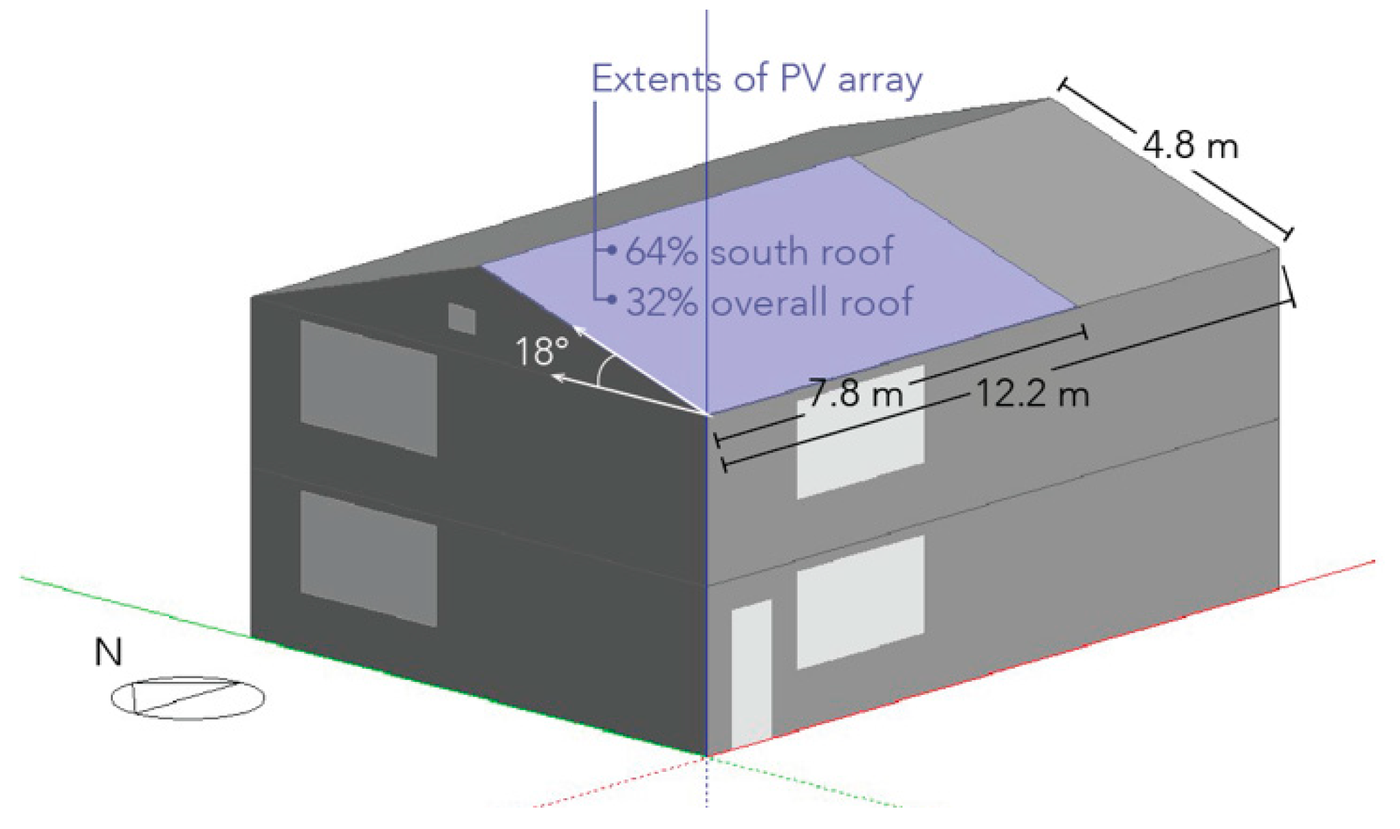
2.2.5. Renewable Energy Retrofit, Operational Energy Assumptions
Per Table 3, each renewable energy case assumed a 7.15 kW PV system with 23 panels and a system efficiency of 19.7% [31].
The modeled extents of the PV array are illustrated in Figure 2. Though the energy model includes PV on the south-facing roof surface, one could generate a comparable amount of electricity to that of the modeled PV array via a different roof orientation by increasing the size of the array. Monetary costs and embodied emissions associated with the PV array were all based on a south-facing array. The impacts of different roof orientations on solar radiation and PV electricity generation are illustrated further in Section S5 of the Supplementary Materials.
Figure 2.
Extents and placement of PV array in DesignBuilder energy model.
2.2.6. Energy Simulation
Using the inputs and methods described in Section 2.2.1, Section 2.2.2, Section 2.2.3, Section 2.2.4, and Section 2.2.5, the authors ran an energy simulation in DesignBuilder for each retrofit intervention with results given in Table 4. Any model parameters not discussed in Section 2 were simulated using the default settings of the original prototype model.
Table 4.
Annual Houston energy simulation results by retrofit case, in site energy (kWh).
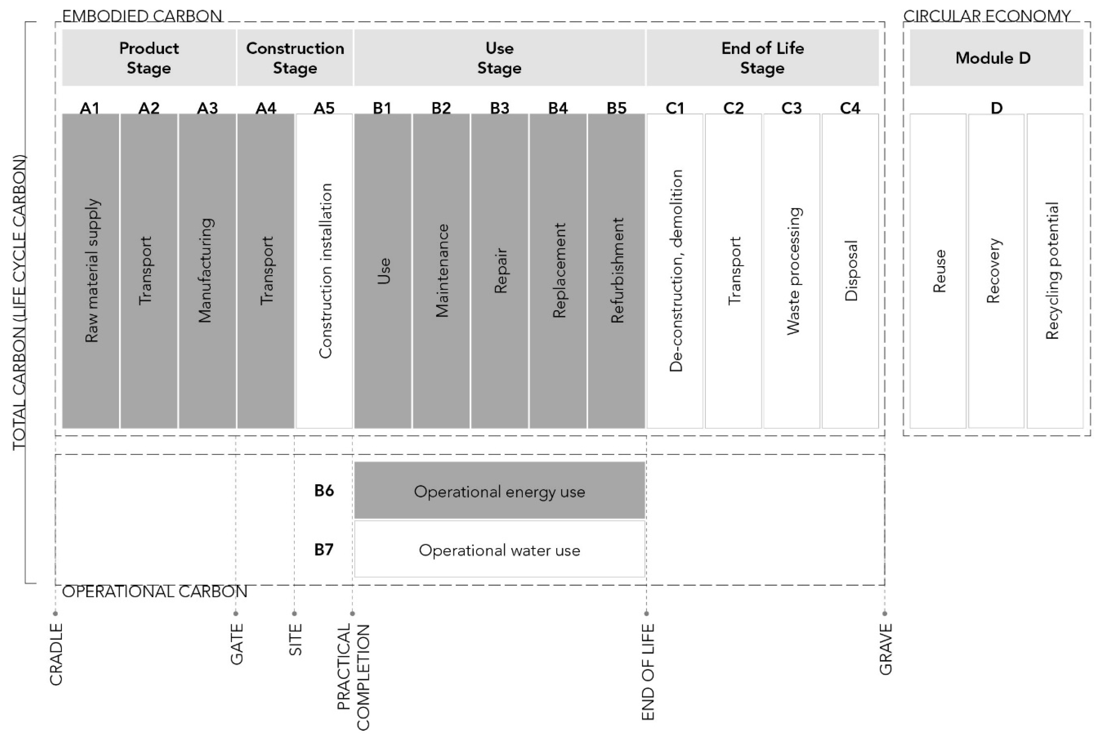
2.3. Whole-Life Carbon
This portion of the study uses Life Cycle Assessment (LCA) to quantify the embodied carbon from the retrofit upgrades and the operational carbon from the homes’ energy consumption. Summing the embodied and operational carbon yields the whole-life carbon. The LCA methodology is consistent with LCA standards ISO 14040 [32] and ISO 14044 [33]. Also, although the methodology complies with EN 15978:2011 to the greatest extent possible [34], the system boundary for operational energy includes plug loads in order to compare the impacts of electrifying kitchen stoves to the impacts of the other proposed retrofit measures. Figure 3 illustrates the system boundary for the LCA. The functional unit is the retrofit installation along with the operation and maintenance of the home from 2020 to 2050.
Figure 3.
System boundary for LCA of retrofit interventions. Only the shaded stages are included in the LCA scope.
2.3.1. Overview: Estimating Whole-Life Carbon Reductions
Because the base case represents an existing home, for most base case calculations, there are no associated embodied carbon expenditures, and the authors only needed to calculate operational carbon. To do so, they used the Emissions & Generation Resources Integrated Database (eGRID2020) to find emission rates and grid gross loss factors associated with the ERCT (Houston), CAMX (Los Angeles), and RFCW (Chicago) electricity grids [35]. The authors then estimated the emission rates from combined generation and line losses () using Equation (1), published by the U.S. Environmental Protection Agency (EPA) [36]:
where = emission rate to estimate emissions from combined generation and line losses (kgCO2e/kWh);
= eGRID generation-based output emission rate (kgCO2e/kWh);
= eGRID grid gross loss factor (decimal).
The resulting emission rates are provided in Table 5. Emission rates used to assess different policy pathways are provided in Table 6 and described in further detail in Section 2.6. The authors multiplied the combined emission rate () by the base case site energy consumption (kWh) from the energy simulations in Section 2.2.6 and multiplied by the study period of 30 years to calculate the base case’s operational carbon over the analysis period. The authors calculated each retrofit’s operational carbon using the same process.
Table 5.
Grid emission rates for electricity and natural gas.
Table 6.
Electricity grid emission rates for alternative policy pathways in the Houston case [39].
The authors also quantified the carbon emissions associated with the retrofit’s product manufacturing (EN 15978 A1–A3), maintenance (EN 15978 B2–B3), and replacement (EN 15978 B4–B5) [34]. They added these emissions to building operational emissions, then subtracted the sum from the base case operational emissions per Equation (2). The difference represents the retrofit’s reduced global warming potential (GWP) over the study period.
where = retrofit’s reduction in GWP from the base case (kgCO2e);
= base case operational carbon (kgCO2e);
= retrofit’s embodied carbon associated with product manufacturing (kgCO2e);
= retrofit’s embodied carbon associated with maintenance and replacement (kgCO2e);
= retrofit’s operational carbon (kgCO2e).
Using Equation (2) to calculate a retrofit’s whole-life carbon reduction works well for the envelope upgrade and renewable energy scenarios because both involve adding assemblies absent from the base case. The electrification interventions, however, require a slightly different method using Equation (3). For the electrification interventions, the authors assumed that the home’s appliances had reached their end of life, and the homeowner could either replace their existing gas appliance(s) with a higher-efficiency gas appliance (baseline assumption) or they could upgrade to an even more efficient electricity-fueled appliance (electrification retrofit measures). Therefore, calculating GWP reductions for the electrification retrofits requires comparing the manufacturing and maintenance emissions from the base case gas appliances against corresponding emissions from the electric appliance upgrades accounting for product lifespan as outlined in Table 7.
where = base case embodied carbon associated with product manufacturing (kgCO2e);
Table 7.
Appliance assumptions used to conduct the LCA for the base case and electrification cases.
= base case embodied carbon associated with maintenance and replacement (kgCO2e).
2.3.2. Base Case, Whole-Life Carbon Assumptions
Table 8, Table 9 and Table 10 outline the material assumptions and specifications required to reach the target performance values given in Table 1, Table 2 and Table 3 and is used to calculate the embodied carbon associated with the base case and each retrofit intervention, as described further in Section 2.3.3, Section 2.3.4 and Section 2.3.5. For each gas-fueled system in the base case, GWP values were collected from the literature. The sum of the GWP values from all considered life cycle stages is noted in Table 7. The referenced values were taken from LCA studies on residential appliances, and all values were converted to the same functional unit per Section 2.3. Manufacturing GWP values were assumed to be applicable to the U.S. context. All operational emissions were derived by running climate-specific energy simulations, as described in Section 2.2, and multiplying the resulting site energy consumption by the grid emission factor per Section 2.3.1.
Table 8.
Houston electrification retrofit interventions and material assumptions.
Table 9.
Houston envelope retrofit interventions and material assumptions.
Table 10.
Houston energy model renewable energy retrofit interventions and material assumptions.
2.3.3. Electrification Retrofit, Whole-Life Carbon Assumptions
The GWP values for the electric appliances were collected using the same process as was used for the gas appliances in Section 2.3.2, except the authors used Equation (3) to find the retrofits’ GWP reduction. For all baseline gas appliances and upgraded electric appliances, the equipment capacity assumptions are given in Table 8 and used to find realistic embodied carbon estimates in the literature. The total GWP from all considered life cycle stages is noted in Table 7.
2.3.4. Envelope Retrofit, Whole-Life Carbon Assumptions
Table 9 shows material assumptions for the shallow and deep envelope retrofits, including fiberglass window frames for windows, cellulose insulation within stud cavities, and rigid insulation (polyisocyanurate) outside of the wall cavities. Using those material assumptions, the authors modeled the prototype home in Revit version 2021 [47], modeling one design option for the base case, one for the shallow envelope retrofit scenario, and another for the deep envelope retrofit scenario, per Figure 4.
Figure 4.
Life Cycle Assessment scope for the envelope upgrade scenarios.
The authors used Tally version 2022.04.08.01, a Revit plug-in that estimates a design’s embodied carbon based on the material quantities in a building information model, to assign materials and emission factors from Tally’s database to the design options [48]. The authors adjusted the GWPs for all insulation and window retrofits over the study period to match the functional unit. All envelope materials analyzed in Tally had lifespans over 30 years, so the authors did not need to factor in carbon emissions associated with product replacement. They omitted emissions associated with end-of-life (EN 15978 C2–C4) and Module D (EN 15978 D) life cycle stages to align with the system boundary per Figure 3 [34].
Quantifying the GWP of the infiltration retrofits in Tally was not possible, so the authors used other methods. For the shallow envelope infiltration case, the authors did not have data for the GWP of air sealing products and assumed the embodied emissions would be negligible. Similarly, for the deep envelope infiltration case, they assumed that the ventilation system addition would be the main source of embodied carbon.
The authors used SimaPro version 9.2.0.2 (EcoInvent 3 library, APOS, and TRACI 2.1 characterization scheme) [49] to estimate the GWP of the ERV unit, motor, and filters based on the Life Cycle Inventory (LCI) from Nyman et al.’s study [50]. Given that the lifespan of an ERV system is typically at least 20 years, the authors assumed one replacement to the ERV unit [51]. Table S72 in the Supplementary Materials outlines the embodied carbon emissions from the ERV units, replacement filters, and motors. Emissions associated with the ERV are aggregated under the “deep envelope” and “deep all” retrofit cases.
2.3.5. Renewable Energy Retrofit, Whole-Life Carbon Assumptions
The authors found the GWP for the PV array as specified in Table 10 using SimaPro (see Table 11). The analysis included the PV panels and inverter. Energy from the PV system was assumed to reduce operational energy (and corresponding operational emissions) up to the home’s electricity demand. Any surplus energy from the PV system was not credited to the residence. The PV panels have a 30-year lifespan, so the authors did not include PV replacement in the analysis [52]. The inverter, however, has a lifespan closer to ten years, so the authors accounted for replacing it twice [53]. Table S73 in the Supplementary Materials outlines further assumptions behind the embodied carbon emissions from the PV array.
Table 11.
Houston data from the energy simulations, LCA, and LCC assessments under current Houston grid emission rates.
2.3.6. Whole-Life Carbon Analysis
Whole-life carbon estimates based on the inputs and methods described in Section 2.3.1, Section 2.3.2, Section 2.3.3, Section 2.3.4, and Section 2.3.5 are given in Table 11. The methodology for estimating upfront costs and Life Cycle Costs is further described in Section 2.4.
2.4. Life Cycle Cost
The authors used the DOE’s methodology to calculate Life Cycle Cost (LCC) for each retrofit [24]. The DOE methodology assumes that homeowners finance the retrofits’ initial investment through increased mortgage costs, but it also accounts for positive and negative cash flows such as the retrofits’ energy savings, replacement costs, residual values, and tax deductions for mortgage interest and property tax payments. Equations (4) and (5) sum costs and savings over multiple years by adjusting all cash flows to the present value assuming a discount rate of 5%; multiple present values representing different cash flows are added together to arrive at the LCC [24]. Equations S7–S14, published by DOE and referenced in Section S8 of the Supplementary Materials, describe how to calculate each cash flow.
where = Life Cycle Cost ($);
= present value ($).
where —annual cash flows at a specified year, y ($);
d = discount rate of 5%.
The authors calculated the upfront cost for each retrofit using a combination of construction cost estimating software. They used Clear Estimates data from 2021 to price building systems and appliances [54]. To price PV systems, the authors assumed $2.65/W [31]. They used RSMeans version 8.7 (Year 2022 Quarter 2) to price most envelope retrofits. However, the authors had to rely on outside sources to estimate costs for triple-pane windows, ERV units, and blower door tests [56,57,58,59].
Retrofits involving infiltration upgrades were especially difficult to price. Although the RSMeans database contained pricing for air barrier materials and installation, it was not clear how the assumed cost of labor related to the target infiltration rate. The authors found that the national average cost to air seal a 140 m2 home ranges from $600 to $2300, with most homeowners paying around $1450 to seal interior and exterior walls [60]. The low-end cost was $200 to air seal ductwork and the high end was $7500 to air seal the basement, attic, and walls. Because the prototype home model is closer to 223 sqm, the authors assumed air sealing would cost approximately $2300 for the shallow infiltration measure, and $7500 for the deep infiltration retrofit [60].
Upfront costs and LCCs for each retrofit case are outlined in Table 11, with further details on energy cost assumptions in Section S8.3 of the Supplementary Materials. Although many programs offer incentives for energy retrofits, no incentives were included in this analysis. By omitting current incentives in pricing, the results reveal where incentives could be leveraged for the greatest environmental benefits rather than how retrofits with current financial incentives stack up against those without incentives.
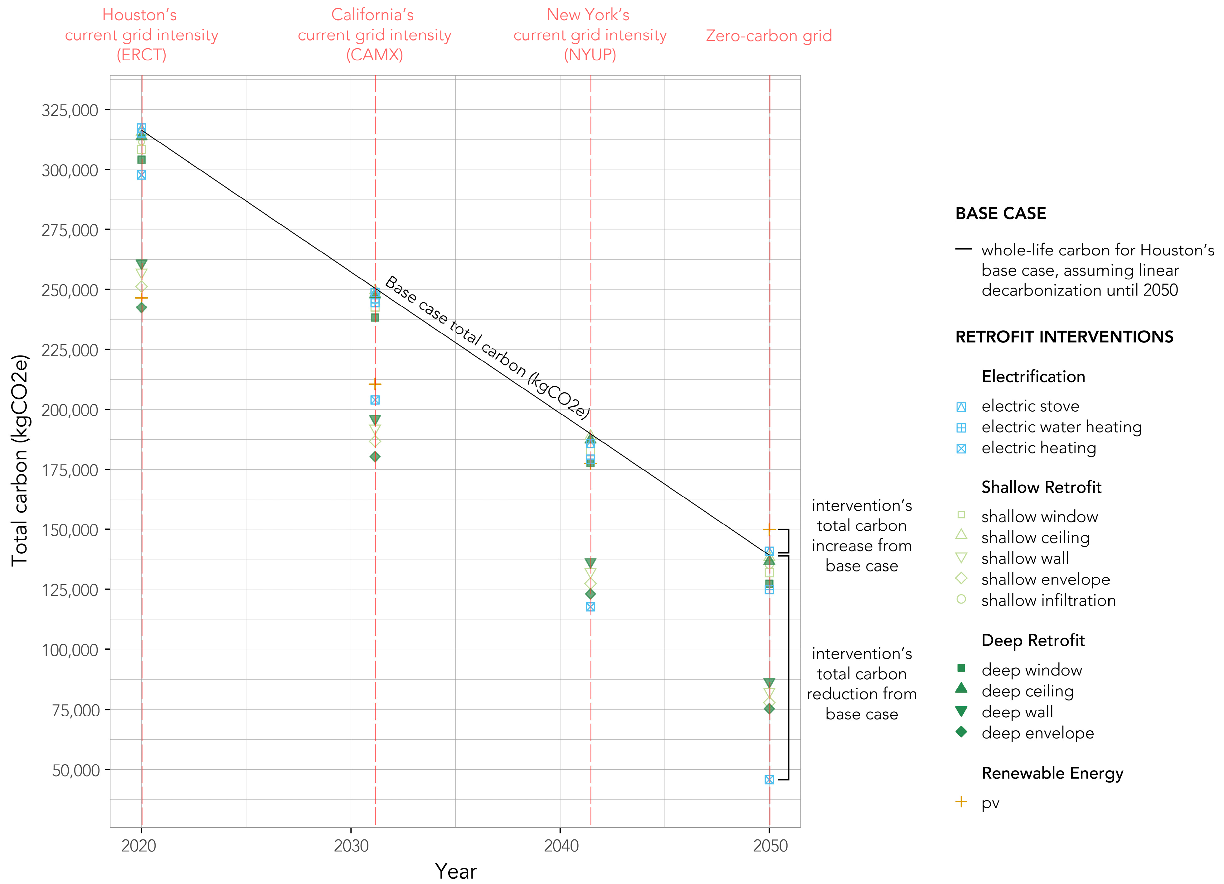
2.5. Decarbonization of the Electric Grid
The authors calculated life-cycle emissions for the base case and each retrofit using a constant grid emission rate for the life cycle of the building (see Table 5). This calculation was repeated for four different grid emission rates to estimate how the retrofit rankings would differ if the make-up of the electric grid were more or less carbon intensive. Below are the four grid emission rates evaluated, using the Houston case as an example:
- Retrofits’ carbon emissions are estimated at Houston’s current grid intensity (0.393 kgCO2e/kWh).
- Houston’s grid is assumed to be as carbon intensive as California’s current grid (0.247 kgCO2e/kWh).
- Houston’s grid is assumed to be as carbon intensive as New York’s current grid (0.112 kgCO2e/kWh).
- Houston’s grid is assumed to have net-zero emissions.
The authors multiplied the site energy consumption for the base case and retrofit interventions by the emission rates above to calculate the estimated operational carbon for each case. As in Section 2.3.1, the authors then found the whole-life carbon reduction resulting from each retrofit intervention using Equation (2) or Equation (3).
Comparing each retrofit intervention back to the base case, each retrofit was ranked according to two separate metrics: (1) reduced source energy (kWh) per dollar spent (or saved) and (2) reduced whole-life carbon (kgCO2e) per dollar spent (or saved). Using the second metric, each ratio had four possible outcomes. To rank among them, the authors created a hierarchy where retrofit interventions that fall under outcome 1 have the highest (best) rankings, and interventions under outcome 4 have the worst rankings: (1) the retrofit decreased carbon at a cost savings, (2) the retrofit decreased carbon at a cost expenditure, (3) the retrofit increased carbon at a cost saving, and (4) the retrofit increased carbon at a cost expenditure.
2.6. Alternative Policy Pathways
Many uncertainties surround how changes in policy, technology, and economics will cause grid emissions rates to shift in the future. To understand how different policy pathways could impact the retrofit rankings, in addition to the grid emissions investigations described in Section 2.5, the authors also utilized the National Renewable Energy Laboratory’s (NREL’s) 2024 Standard Scenarios, which have been designed to capture a range of potential futures and estimate the fuel make-up of U.S. electrical grids over time [39]. Using the emission rates in Table 6, the authors compared life-cycle emissions for different retrofits under the following scenarios in the years 2032 and 2050:
- The “Mid-Case with no Inflation Reduction Act (IRA) or Clean Air Act Section 111 (CAA) Scenario” does not include IRA electric sector tax credits nor the updated CAA rules.
- The “Mid-Case Scenario” has median values for inputs like technology and fuel prices, resource availability, demand growth, availability of nascent technologies, and the future policy environment.
- The “High Natural Gas Cost Scenario” assumes higher natural gas costs than median projections.
The change in retrofit rankings resulting from this analysis are documented in Section 3.1.
2.7. The Time Value of Carbon
The TVC is the concept that reductions in carbon emissions today are more valuable than the same reductions in the future due to the compounding damages of GHG emissions. This concept has been referenced in policy efforts to establish a Social Cost of Carbon (SCC) but is seldom used in the building industry. The discount rate used in SCC calculations determines how much weight is placed on future emissions, with a high discount rate signaling that future emissions are less significant than present emissions [19]. Though there is not yet consensus on one appropriate discount rate (or even one discounting method), federal regulatory analysis for carbon pricing has used discount rates of 3% and 7% [18,61].
The authors conducted a sensitivity analysis by applying each discount rate to the carbon emissions from each base and retrofit case. Using each city’s current grid emission rate, they listed the building’s carbon emissions for each year from 2020 to 2050 for each retrofit intervention. Annual emissions always included the home’s operational carbon for the year. In addition, the year 2020 always included the embodied emissions from the retrofit’s materials. Additional embodied emissions were added when the product lifespan elapsed, representing the embodied carbon from product replacement. Some retrofit interventions also had regular embodied emissions associated with product maintenance. Once the whole-life carbon emitted in each year of the analysis period had been calculated, the authors used Equation (6) to convert future damages (carbon emissions) into present-day values and summed the emissions over the study period.
where = whole-life carbon present value associated with retrofit intervention over the study period (kgCO2e);
= number of years in the analysis period (30 years);
= whole-life carbon associated with retrofit intervention at a specified year, y (kgCO2e);
= discount rate of 3% or 7%.
3. Results
The purpose of the following analysis is to demonstrate how the details of metrics used (whether it is energy or carbon), grid carbon intensity, policy pathway, or the TVC impact the rankings of home retrofit options.
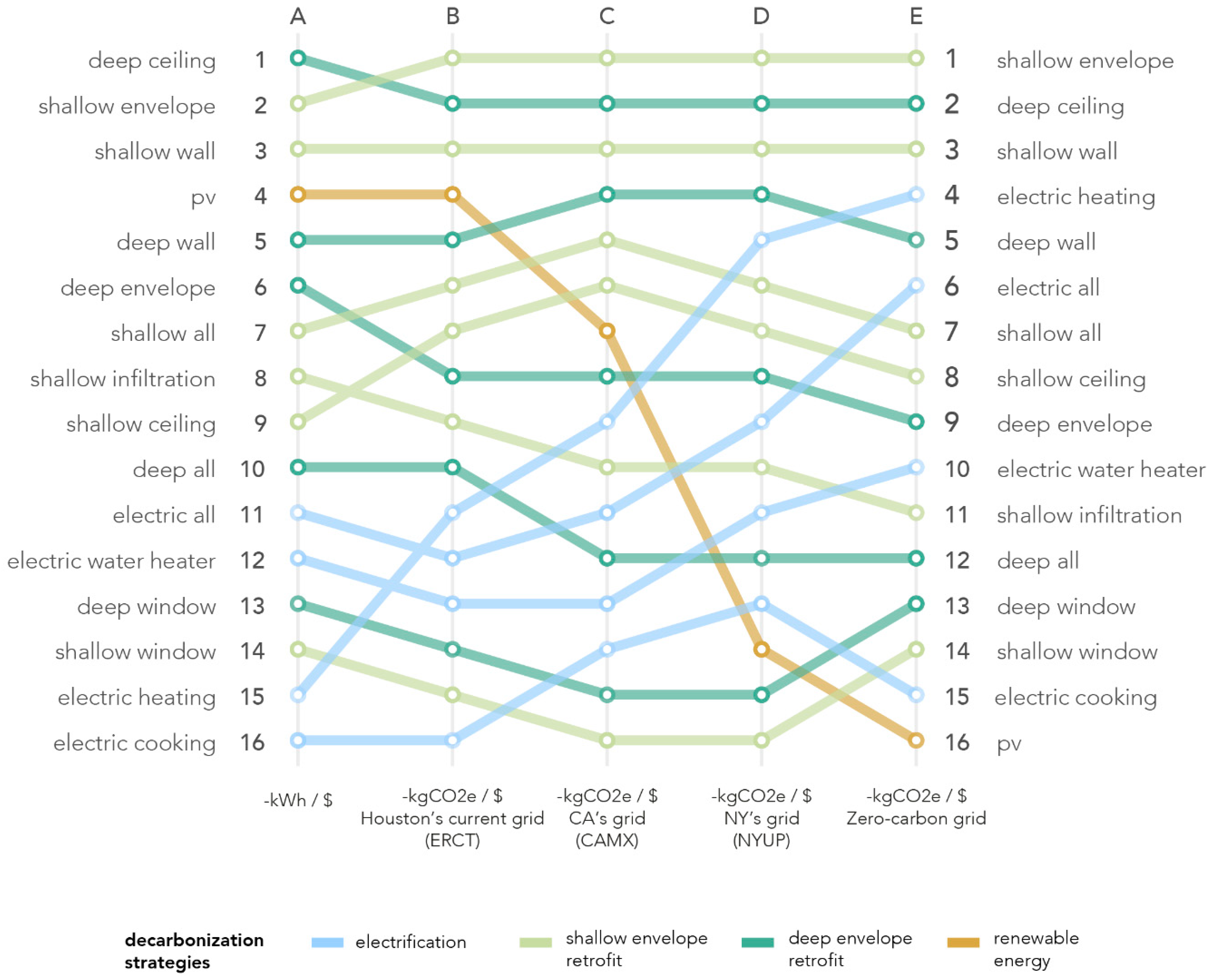
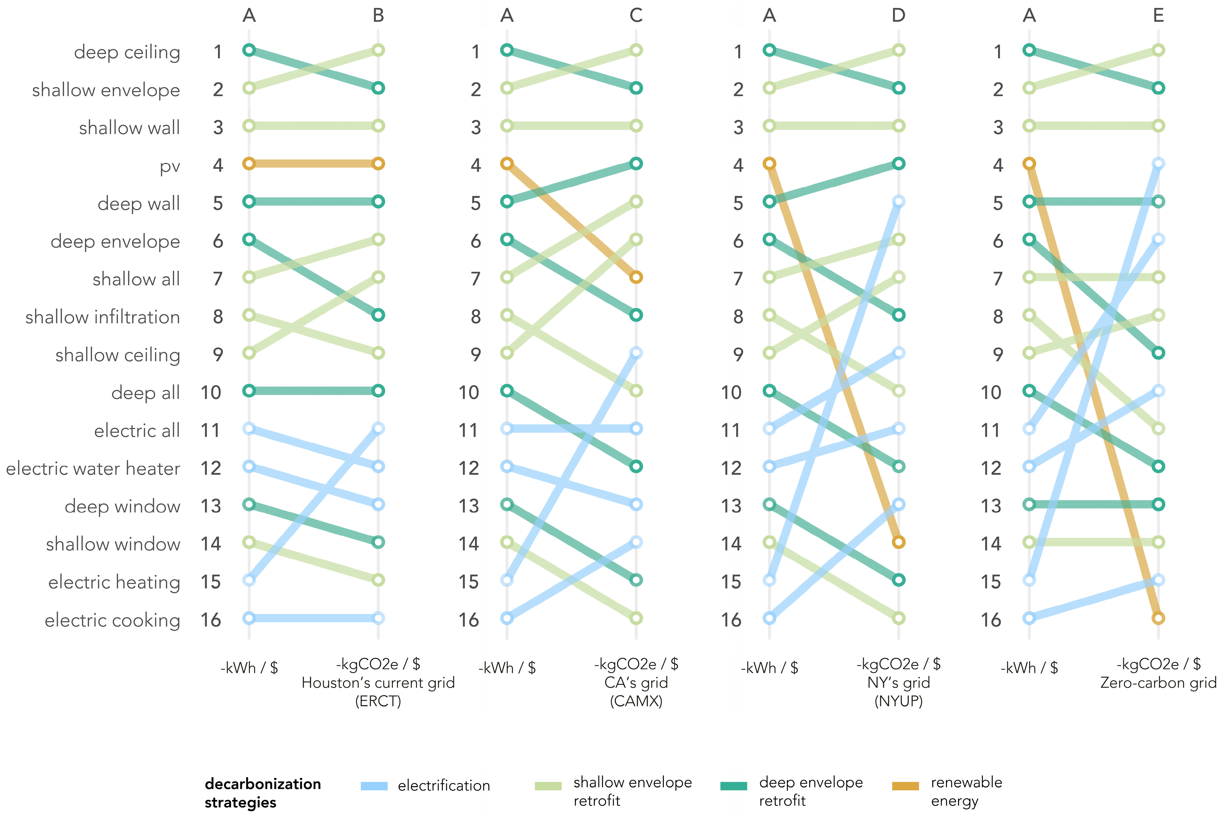
3.1. Ranking of Retrofit Interventions as the Electrical Grid Decarbonizes
Rankings for each retrofit intervention under the current Houston grid, California’s grid, New York’s grid, and a zero-carbon grid are outlined in Table 12 and graphically displayed in Figure 5. As seen in Figure 5, electrification retrofits, except for electric cooking, tend to rank higher on grids with lower carbon intensities. Considering Houston’s current grid, the PV intervention ranks fourth. However, with the current grid emission rate of New York’s grid, the PV intervention for the Houston home ranks fourteenth. Shallow and deep retrofits do not drastically change position, and when they do, it seems to be because other retrofit interventions are trending up or down in rank.
Table 12.
Reduced energy and carbon emissions associated with each retrofit intervention in Houston. Retrofit interventions are ranked from best (1) to worst (16) considering increasingly decarbonized grids.
Figure 5.
Ranking of retrofit interventions from best (1) to worst (16) considering increasingly decarbonized grids.
Figure 5 also displays results using the more typical metric of reduced source energy per dollar spent. When comparing between the energy metric (-kWh/$) in column A and the whole-life carbon metric (-kgCO2e/$) in column B for Houston’s current grid intensity, the difference in rankings is noticeable, but not extreme. However, as one considers grids with lower carbon intensities, the retrofit rankings based on emissions change substantially. Using the whole-life carbon metric yields entirely different results over time, especially when comparing between columns A and E. Key takeaways from these results are discussed further in Section 4.1.
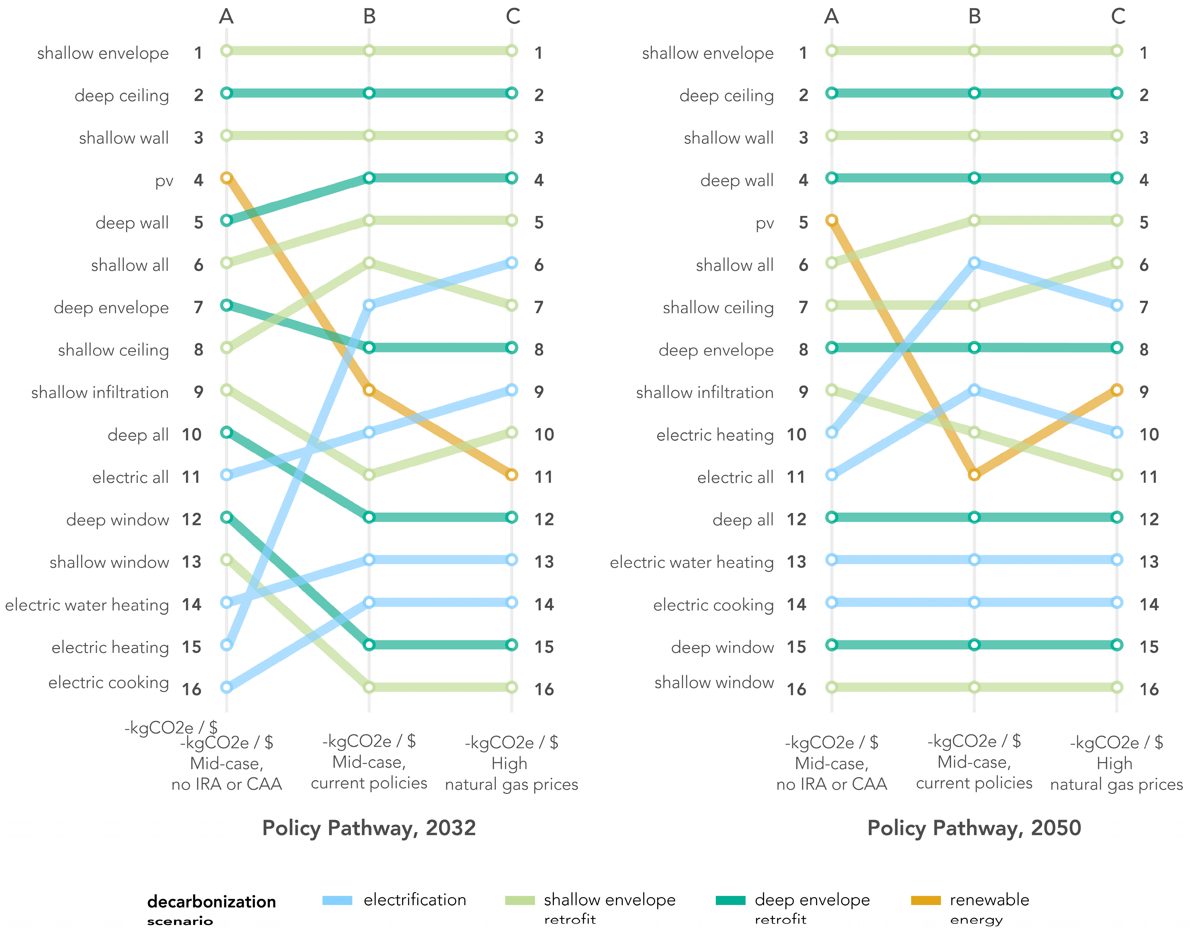
3.2. Retrofit Rankings Under Alternative Policy Pathways
The authors also estimated the change in retrofit rankings in Houston under three policy pathways in 2032 and 2050, with the results documented in Table 13 and visualized in Figure 6. Here, the policy pathways are arranged from higher (on left) to lower (on right) electric grid emission rates. Figure 6 exhibits similar trends to those observed in Figure 5, with electrification decarbonization scenarios generally improving in rank and renewable energy scenarios generally falling in rank with policies that incentivize electric grid decarbonization.
Table 13.
Reduced energy and carbon emissions associated with each retrofit intervention in Houston under alternative policy pathways. Retrofit interventions are ranked from best (1) to worst (16).
Figure 6.
Ranking of retrofit interventions from best (1) to worst (16) under alternative policy pathways in Houston in 2032 and 2050.
Figure 6 also illustrates that prioritizing building retrofits based on current conditions can lead to significantly different recommendations than if the policymaker or homeowner were setting priorities based on a different implementation year or under a different policy pathway altogether. The implications of the retrofit rankings’ high sensitivity to policy assumptions are discussed further in Section 4.1.
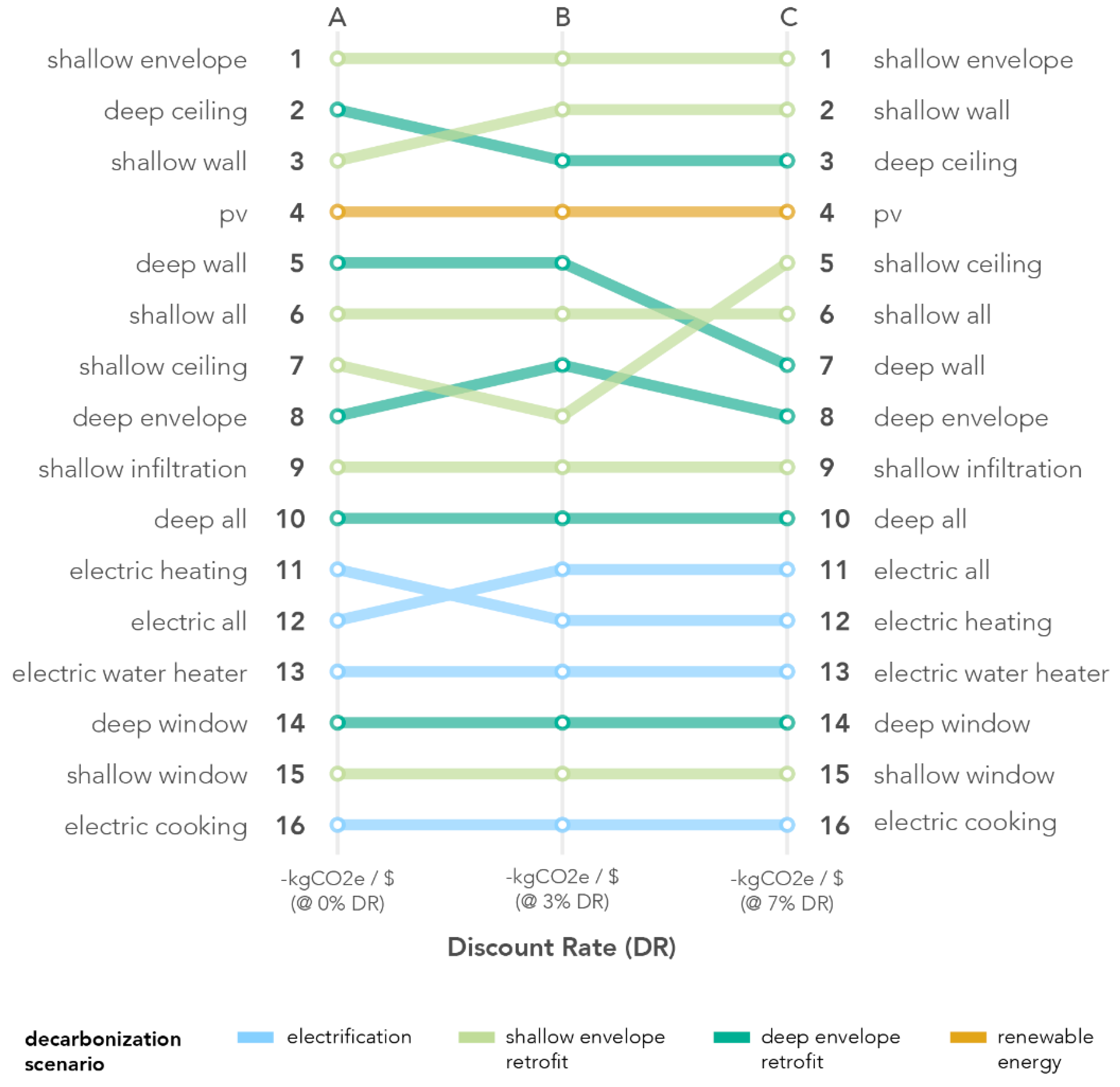
3.3. Retrofit Rankings Accounting for the Time Value of Carbon
The results from ranking the Houston retrofit interventions, considering different carbon discount rates (and assuming Houston’s current grid emission rate remains constant over the full study period) are shown in Table 14, with a graphic representation in Figure 7. The change in rankings among the different carbon discount rates can be attributed to differences in a product’s initial embodied carbon expenditure, how often the products need to be replaced, and when embodied emissions are “spent” over the product’s lifespan.
Table 14.
Reduced energy and carbon emissions associated with each retrofit intervention in Houston, accounting for the time value of carbon. Retrofit interventions are ranked from best (1) to worst (16) under Houston’s current electric grid as the carbon discount rate increases.
Figure 7.
Ranking of Houston retrofit interventions from best (1) to worst (16) considering the time value of carbon and three different assumptions of carbon discount rate.
In Figure 7, as the carbon discount rate increases from column A to C, shallow retrofits either maintain their ranking or move up in rank. Those that move up in rank (shallow wall and shallow ceiling insulation) utilize extremely low-carbon materials like cellulose insulation, resulting in proportionally greater carbon reductions than higher-carbon retrofits when the discount rate is applied. Meanwhile, some of the deep retrofits (deep ceiling insulation, deep wall insulation, and deep envelope) decline in rank because they rely on higher-carbon exterior insulation and require wall cladding replacement. The same is true for electric heating with its high initial embodied carbon from the system’s refrigerants.
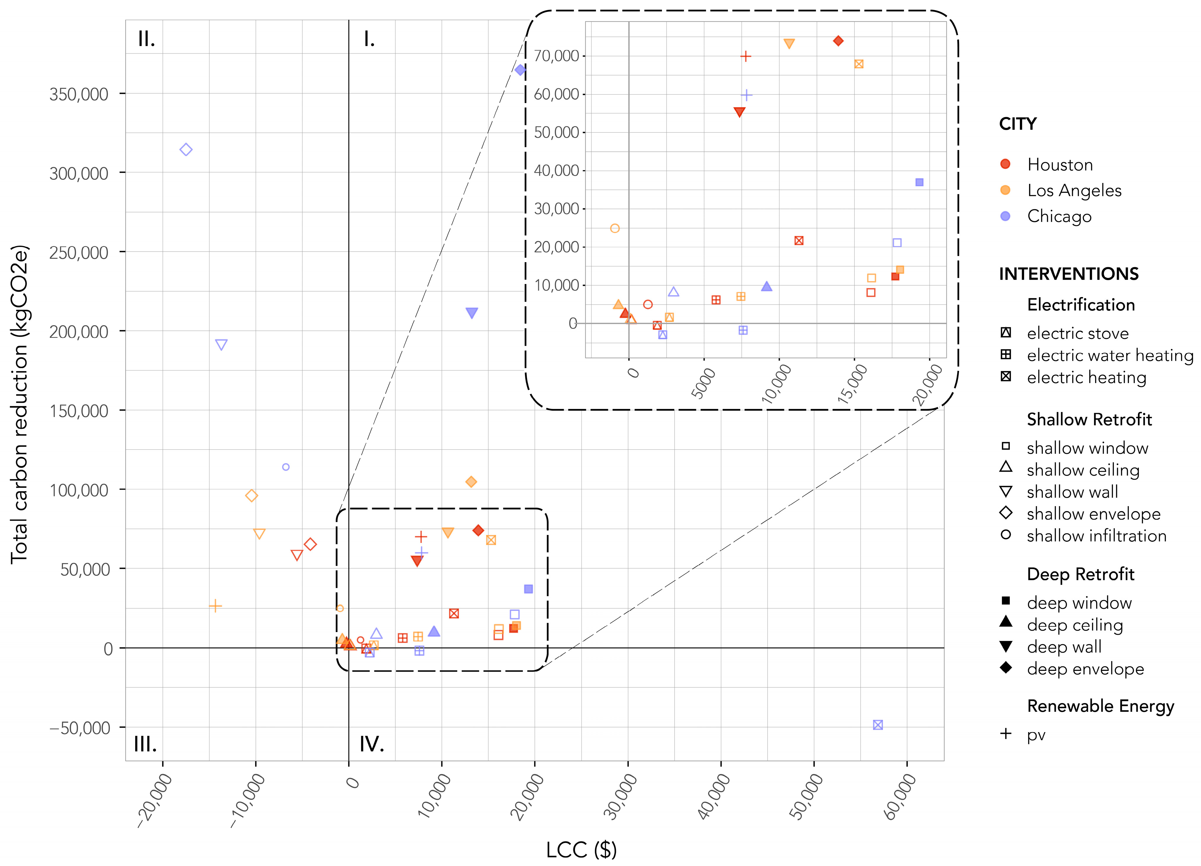
3.4. Carbon Emissions and Associated Costs
The authors also provided the results in terms of whole-life carbon per LCC. As shown in Figure 8, of the eleven retrofit interventions that fall in Quadrant II (representing carbon reductions at a cost savings), eight of them belong to the shallow retrofit scenario, and the only shallow retrofit interventions that do not provide cost savings over the course of the analysis period are the window upgrades and addition of ceiling insulation. This suggests that existing homes without proper insulation and air sealing can see significant carbon and cost reductions from addressing these issues.
Figure 8.
Whole-life carbon reduction versus LCC of retrofit interventions by city.
Homes with the highest energy consumption to begin with, e.g., in Chicago’s cold climate, stand the most to gain from energy retrofits. As shown in Figure 8, the whole-life carbon reductions resulting from upgrades to the Chicago home, especially the envelope upgrades, far surpass those from the homes in Los Angeles or Houston. However, homes in Chicago also saw the greatest increases in carbon emissions from the electrification retrofits due to the high emissions intensity of Chicago’s grid (assuming these emission rates remain steady into the future). Therefore, if targeting geographical regions to prioritize carbon reductions, logic suggests starting in cold climates, but strategically. For instance, in Chicago, it may make sense to tackle shallow retrofits, and even some deep retrofits, over electrification—depending on one’s confidence in Chicago’s future grid decarbonization over the life of the retrofit.
As shown in Figure 8, the electrification retrofits in Los Angeles, particularly the switch from gas furnaces to air-source heat pumps, make more sense from a carbon-standpoint than they would for the other two cities because California’s grid already has a relatively high percentage of renewables. However, according to the assumptions used here, the LCC for the electric heating retrofit in Los Angeles is high. In Los Angeles, PV upgrades make sense from a financial perspective, but, according to these calculations, they do not reduce as much carbon as many of the other retrofit interventions.
3.5. Carbon Emissions over Time
The results presented in Figure 9 illustrate the retrofits’ whole-life carbon emissions as the grid decarbonizes without considering cost. Such results could help guide programs targeting the greatest possible carbon reductions and determine where it is most logical to subsidize retrofit measures. Figure 9 plots whole-life carbon emissions against time for the Houston retrofits under Houston’s current grid mix. Beyond 2020, the city’s grid intensity decreases, assuming linear decarbonization, until it reaches zero-emissions in target year 2050.
Figure 9.
Whole-life carbon associated with Houston retrofit interventions. This graph shows whole-life carbon for the base case and each retrofit intervention using a constant grid emission rate for the life cycle of the building. The calculation is repeated for four different grid emission rates.
In Figure 9, retrofit interventions furthest below the base case line represent the greatest carbon emissions reductions (and those above the base case represent a slight increase in carbon emissions). Based on the findings in Houston, the wall insulation and overall envelope upgrades (both shallow and deep retrofits) consistently provide substantial carbon savings. Some retrofits drastically change position relative to other retrofits as the grid decarbonizes. For instance, the electric heating retrofit initially provides low- to mid-range carbon reductions relative to the other retrofit interventions. However, as the grid decarbonizes, the switch from gas to electric heating quickly becomes the retrofit measure with the greatest carbon reduction potential.
4. Discussion
4.1. Contributions
This study demonstrates the potential impact of broadening the scope of carbon calculations in building retrofits. This paper presents a methodology to compare monetary costs and environmental benefits among decarbonization strategies at various grid intensities, with different policy pathways, and at different time values of carbon. Figure 10 compares the shift in the Houston case’s retrofit rankings when using the typical metric of reduced energy per dollar spent (-kWh/$) in column A to the proposed metric of reduced carbon per dollar spent (-kgCO2e/$) in columns B, C, D, or E. The difference in rankings is fairly minor when looking at Houston’s current grid (column B), but the differences are more pronounced moving from left to right as each grid is less carbon intensive. This pattern suggests that the whole-life carbon metric will become even more important as electricity grids continue to decarbonize.
Figure 10.
Houston retrofit rankings’ widening discrepancy over time between the more typical metric of reduced energy per dollar spent (-kWh/$) and the proposed metric of reduced carbon per dollar spent (-kgCO2e/$).
The rankings of distinct retrofit interventions vary from city to city, but the general trends in how the three decarbonization strategies perform over time are relatively consistent across the three cities and three alternative policy pathways studied, as shown in Figures S1, S3, and Figure 6. Assuming current grid emission rates, envelope retrofits tended to rank better than renewable energy and electrification upgrades in terms of kgCO2e per dollar spent. However, as grid emission rates decreased, electrification upgrades rose in rank, while renewable energy upgrades fell.
While the results suggest that adding PV will make less of an impact as the grid decarbonizes, this finding poses a paradoxical challenge. Achieving a cleaner grid is impossible without implementing low-carbon energy generation, such as PV. Thus, these results should not be interpreted to imply that PV retrofits are undesirable. Rather, this exercise demonstrates how design priorities may shift in a changing context. Similarly, the change in retrofit ranking, depending on the policy pathway and the year of implementation, as described in Section 3.2, highlights the flaws in decision-making that can occur when decision-makers only have data based on existing policies and current grid emission rates.
Accounting for the TVC, as described in Section 2.7, generally caused retrofits with high initial carbon to drop in ranking. However, in studies on building performance, the TVC is rarely quantified. As a result, studies that do consider whole-life carbon from buildings assume a carbon discount rate of 0% by default. Limitations to this study’s TVC approach are further described in Section 4.2, with recommendations for future study in Section 4.3. Even still, and although there is not yet a consensus on what the correct discount rate should be, logic suggests that it is probably not 0%. Therefore, assuming there is no discount rate or other approach to the TVC can misinform retrofit decision-making.
Furthermore, shifts in rankings as the authors’ assumed carbon discount rate increases, do not follow the same patterns observed as the grid decarbonizes. This finding suggests that whole-life carbon and the TVC have important implications for designers, policymakers, and homeowners who make decisions about building decarbonization and the timing of decarbonization approaches, especially in cases where future carbon savings require a large up-front output in embodied carbon emissions.
Homeowners can use the reduced carbon per dollar spent rankings to approximate the best retrofit investments for their specific home and budget. The results can also help homeowners decide when it makes sense to replace gas equipment with electric equipment. For instance, in this study’s electrification scenarios, the switch to electric equipment is assumed to take place in 2020. However, in locations with more carbon-intensive grids, it may be less urgent for homeowners to replace their gas-fueled equipment until the anticipated grid emission rate during the expected life of the equipment is low enough for electric equipment to have lower environmental impacts. This conclusion stems from a strict carbon-emission perspective. The end of life of existing equipment and goals beyond carbon accounting, such as promoting market adoption, driving technological innovation, and avoiding technological lock-in, could promote an early adoption of electrification.
Implementing whole-life carbon metrics into building performance analysis would enable researchers, policymakers, and designers to be more strategic with their building decarbonization targets and recommendations. Embodied carbon, grid decarbonization, and the time value of carbon are often omitted from studies that focus on building performance, but these parameters matter. Consideration of these factors changed the predicted carbon emissions and the identification of the highest performing design interventions. The findings suggest that analysts, especially those supporting building policy or incentive programs, should include such considerations.
4.2. Limitations
This study analyzed individual retrofits, such as upgrading the wall insulation, rather than combined retrofits (e.g., both retrofitting the envelope and electrifying the heating system). It is important to note that the benefits are not additive. For example, if retrofitting the envelope lowers the heating load, then the carbon-saving impact of electrifying the heating system would be reduced, and vice versa. For real-world projects, multiple upgrades should be modeled together.
Trends in building emissions from the different decarbonization strategies were consistent across cities, but individual retrofit results were more sensitive to assumptions made in the energy simulations, LCA, and LCC assessments. Ceiling retrofits, for example, ranked lower than expected, likely due to assumptions about existing attic insulation in the base building. While adding additional ceiling insulation was not a top priority in the studied cities, it would be an important investment for homes with no existing ceiling or roof insulation. Other practical considerations, like ease of installation and disruption to occupants, could encourage retrofits in unoccupied spaces like attics.
Air infiltration ranking depended heavily on labor cost assumptions, which vary widely due to the range of conditions in existing homes. If labor estimates were too low, the infiltration retrofits may have been overvalued. Similarly, methodological decisions around ground modeling and mechanical system designs, as discussed in Sections S2.3 and S4.4 of the Supplementary Materials, could be further developed to improve the accuracy of the results.
The assumption of one stable grid emission rate from 2020 to 2050 was used for simplicity, though real-world grids will likely decarbonize over time. If a dynamic rate had been used, the differences between each grid decarbonization scenario would be less pronounced, as all would approach the same zero-carbon target by 2050.
Notably, applying a discount rate to estimate the TVC for building materials may have limitations. Whole-life carbon results in this paper are expressed in terms of global warming potential over 100 years. Because the gases that lead to global warming stay in the atmosphere for different lengths of time, GWP(100) is already a time-weighted value [62]. Therefore, some argue that applying a “carbon discount rate” to an already time-weighted metric may result in an over-counting of carbon reductions (one study estimates that a 100-year GWP timescale is consistent with a discount rate of 3.3%) [63]. A somewhat improved alternative would be using GWP(20) data, but limited data exists for building materials.
Additionally, relying on two databases to estimate upfront costs introduced discrepancies between similar materials. To minimize such discrepancies, the authors used RSMeans for all envelope retrofits and Clear Estimates for all equipment retrofits, but still there is a large range of conditions in existing homes, and the study makes a number of assumptions about the existing conditions and assemblies in these homes. Though the results presented are meant to serve as a rough guideline and illustrate general trends, the results may vary widely on a case-by-case basis.
The authors ran into similar challenges when estimating embodied emissions using Tally, the academic literature, and SimaPro. Tally and SimaPro rely on different LCA databases for carbon emission factors. Further, there are numerous ways of estimating embodied emissions within SimaPro, and the method used is not always clear in the literature. This uncertainty in LCA calculations may be one reason that many building policies and programs avoid combining embodied and operational emissions or ignore embodied emissions altogether. Here, the authors take the position that an imperfect estimate is likely an improvement over ignoring an input altogether. With greater resources, all retrofit interventions could be evaluated in SimaPro, increasing the accuracy of the results.
To simplify the analysis, the authors did not consider geographical variations in grid emission rates for embodied carbon calculations, which can have a significant impact on total emissions, especially for PV systems [64]. Additionally, as electricity grids decarbonize, one could reasonably assume that future manufacturing, transportation, and other practices included in LCA will decarbonize to some extent. However, due limited data, these future reductions were not modeled, potentially overstating whole-life carbon emissions in future retrofits.
Due to the lack of available LCA data and to ensure consistency, end-of-life (EOL) emissions were not included in the project scope. Though this data were available for most of the envelope upgrades, the authors did not find comparable data in the literature for the building systems. Figure 11 references the emissions included and excluded for the envelope upgrade scenarios to illustrate the potential impacts from omitted life cycle stages.
Figure 11.
Global warming potential of envelope upgrade scenarios by life cycle stage.
Further, some of the embodied carbon estimates using Tally yield net negative GWPs due to assumed carbon sequestration in the product stage. Per ISO 21930-2017, products that sequester carbon with negative emissions in A1-A2 should release the positive emissions back to the environment in life cycle stages A1, A5, and C3-C4 [65]. Our results do not account for sequestered carbon being released back to the atmosphere at the end of life per ISO 21930-2017. Therefore, the GWP of bio-based materials tend to be lower using Tally than they would be if following the ISO standard, which could overstate the performance of retrofits with biogenic carbon.
4.3. Future Work
Future work should use ISO 21930-2017 to account for a net neutral biogenic carbon balance. Additionally, including emissions from the EOL and Module D life cycle stages would provide a more complete picture of whole-life carbon trade-offs and build a stronger case for working toward closed-loop systems and manufacturing processes. Accounting for an electricity grid’s specific emission rate by manufacturing location in embodied carbon calculations would reveal what portion of emissions result from manufacturing processes versus manufacturing location and identify priorities for whole-life carbon reductions, such as sourcing materials made with less carbon-intensive grids.
Future work should also consider the carbon investment needed to support a large-scale shift to electrification and decarbonizing the electricity grid. This study assumes no electric service upgrades, but individual homes and interconnected grids will require significant infrastructure upgrades to handle higher electricity loads. These upgrades, often requiring extraction of rare earth elements, can have disproportionately large environmental impacts compared to more widely available materials [66].
Ideally, future research would also account for impacts on peak loads, time variable emissions, energy storage opportunities, and associated impacts on electricity costs. Time-of-use pricing can impact both the cost and carbon intensity of the electricity used, but such practices are still not widely implemented for residential customers [67]. Optimizing residential electricity demand timing could better align energy supply and demand, with additional benefits not included here, such as reduced or delayed infrastructure investment and associated embodied emissions.
Section 4.2 addressed the limitations of maintaining one grid emission rate from 2020 to 2050 for each grid decarbonization scenario. Future work could also consider the life of the design decision. For example, if the analysis period remained at thirty years, insulation might be assumed to last the full thirty years, whereas a heat pump might be assumed to last for about 14 years. Therefore, only the grid emissions over the next 14 years would be included in the heat pump analysis, which would make heat pumps less attractive in grids expected to maintain a relatively high carbon intensity over that equipment life.
Lastly, the TVC analysis is built upon a methodology used in setting the SCC. This method was not specifically designed to be applied to emissions. Further methodology development exploring a wider range of discount rates in more cities with different electric grid emission rates could inform a discount rate more appropriate for use with building-related emissions that are typically expressed in GWP100. Work in this realm should consider the discount rate’s consequences on future generations.
5. Conclusions
This research analyzed the carbon- and cost-effectiveness of three decarbonization strategies in residential retrofits of pre-1980s homes in Houston, Los Angeles, and Chicago. The decarbonization strategies—electrifying buildings, upgrading envelopes, and adding renewable energy—were further divided into distinct retrofit interventions in a methodology to help prioritize energy upgrades for different climates, electricity grids, and potential policy pathways. Using energy simulation and LCA, the authors quantified the whole-life carbon reduction and LCC associated with each retrofit, ranked the interventions accordingly, and calculated how the rankings would change if electricity grid emission rates decreased or if decision-makers accounted for the TVC.
Assuming current grid emission rates, envelope retrofits tended to rank better than renewable energy and electrification upgrades. However, as grid emission rates decreased, electrification upgrades rose in rank, while renewable energy upgrades fell. In analyses considering grid decarbonization and future policy pathways, PV and electric heating retrofits changed the most in rank. Out of 16 retrofit interventions ranked from best (1) to worst (16) by carbon emissions per dollar spent, PV retrofits declined from ranking fourth under Houston’s current electricity grid to ranking 14th if Houston’s grid reduced in carbon intensity to the level of New York’s. Electric heating improved from ranking 11th with Houston’s current grid to ranking fifth under New York’s grid emission rate. Including the TVC generally caused retrofits with high initial carbon investments to drop in ranking.
The sensitivity of embodied emissions due to uncertainty in embodied carbon data and variation in electricity grids was not explored in this paper and represents an important area for future research. Still, the results illustrate that considering whole-life carbon, changes in policy, and the TVC changed the predicted carbon emissions and the identification of highest-performing retrofits. The findings suggest that analysts, especially those supporting building policy or incentive programs, should include these considerations in their methods.
Supplementary Materials
The following supporting information can be downloaded at: https://www.mdpi.com/article/10.3390/su17072935/s1, Section S1. Graphed results; Section S2. EnergyPlus/DesignBuilder Calibration for the 2006 Prototype Model; Section S3. Energy simulation parameters for the base (pre-1980s) and retrofit models; Section S4. Estimated solar radiation and energy generation from solar array; Section S5. Energy simulation results; Section S6. Whole-life carbon assumptions and results; Section S7. Life Cycle Cost calculations; Section S8. Grid decarbonization results; Section S9. Time value of carbon results; Section S10. Ranking of retrofit results [68,69,70,71,72].
Author Contributions
Conceptualization, A.H. and H.W.S.; methodology, A.H. and H.W.S.; validation, A.H. and H.W.S.; formal analysis, A.H.; investigation, A.H.; data curation, A.H.; writing—original draft preparation, A.H.; writing—review and editing, H.W.S.; visualization, A.H.; supervision, H.W.S.; funding acquisition, A.H. and H.W.S. All authors have read and agreed to the published version of the manuscript.
Funding
This work received funding from the Harvard Joint Center for Housing Studies, the Harvard Graduate School of Design, and RDH Building Science.
Institutional Review Board Statement
Not applicable.
Informed Consent Statement
Not applicable.
Data Availability Statement
Data are contained within the article and Supplementary Materials.
Acknowledgments
In addition to the funding partners listed above, the authors would like to thank our mentor and colleague, Jonathan Grinham, who provided valuable feedback on the Life Cycle Assessment standards for biogenic carbon.
Conflicts of Interest
The authors declare no conflicts of interest. The sponsors had no role in the design, execution, interpretation, or writing of the study.
Abbreviations
| Abbreviations | Meaning |
| AC | Air conditioning |
| ACH | Air changes per hour |
| ACH50 | Air changes per hour at 50 Pascals of pressure differential |
| ACHnat | Air changes per hour under natural, or normal, operating conditions |
| ASHP | Air-source heat pump |
| ASHRAE | The American Society of Heating, Refrigerating and Air-Conditioning Engineers in America |
| CAA | Clean Air Act Section 111 |
| CAMX | The eGRID sub-region for most of California |
| COP | Coefficient of Performance |
| DC | Direct current |
| DOE | Department of Energy |
| EC | Embodied carbon |
| eGRID | Emissions and Generation Resource Integrated Database |
| EIA | U.S. Energy Information Administration |
| EN 15978 | European Standard 15978 |
| EOL | End of life |
| EP | EnergyPlus |
| EPA | Environmental Protection Agency |
| ERCT | The eGRID sub-region for most of Texas |
| ERV | Energy Recovery Ventilator |
| GHG | Greenhouse gas |
| GWP | Global warming potential |
| IDF | EnergyPlus input file |
| IECC | International Energy Conservation Code |
| IRA | Inflation Reduction Act |
| IRC | International Residential Code |
| ISO 21930-2017 | International Organization for Standardization Standard 21930-2017 |
| LCA | Life Cycle Assessment |
| LCC | Life Cycle Cost |
| LCI | Life Cycle Inventory |
| NREL | National Renewable Energy Laboratory |
| NYUP | The eGRID sub-region for most of New York |
| OC | Operational carbon |
| Polyiso | Polyisocyanurate |
| PV | Photovoltaic |
| RFCW | The eGRID sub-region that includes Chicago, Illinois |
| SCC | Social Cost of Carbon |
| SHGC | Solar Heat Gain Coefficient |
| SEER | Seasonal Energy Efficiency Ratio |
| TVC | Time value of carbon |
| U.S., USA | United States of America |
| U-value | The metric for thermal transmittance, measured in W/m2K |
| VT | Visible Transmittance |
| WH | Water heater |
References
- “2015 RECS Survey Data”, U.S. Energy Information Administration. Available online: https://www.eia.gov/consumption/residential/data/2015/ (accessed on 24 April 2022).
- “2018 CBECS Survey Data”, U.S. Energy Information Administration. Available online: https://www.eia.gov/consumption/commercial/data/2018/index.php?view=characteristics (accessed on 24 April 2022).
- “2018 MECS Survey Data”, U.S. Energy Information Administration. Available online: https://www.eia.gov/consumption/manufacturing/data/2018/ (accessed on 24 April 2022).
- “2015 RECS: Overview”, U.S. Energy Information Administration. Available online: https://www.eia.gov/consumption/residential/reports/2015/overview/index.php?src=%E2%80%B9%20Consumption%20%20%20%20%20%20Residential%20Energy%20Consumption%20Survey%20(RECS)-f6 (accessed on 24 April 2022).
- Pombo, O.; Rivela, B.; Neila, J. Life cycle thinking toward sustainable development policy-making: The case of energy retrofits. J. Clean. Prod. 2019, 206, 267–281. [Google Scholar] [CrossRef]
- Rosner, M. Why Did Renewables Become So Cheap So Fast? Our World in Data. Available online: https://ourworldindata.org/cheap-renewables-growth (accessed on 18 April 2022).
- Cluett, R.; Amann, J. Residential Deep Energy Retrofits. ACEEE, A1401. March 2014. Available online: https://www.aceee.org/research-report/a1401 (accessed on 25 April 2022).
- Polly, B.; Gestwick, M.; Bianchi, M.; Anderson, R.; Horowitz, S.; Christensen, C.; Judkoff, R. Method for Determining Optimal Residential Energy Efficiency Retrofit Packages; National Renewable Energy Lab. (NREL): Golden, CO, USA, 2011. [Google Scholar] [CrossRef]
- Less, B.; Walker, I. A Meta-Analysis of Single-Family Deep Energy Retrofit Performance in the U.S.; Lawrence Berkeley National Lab. (LBNL): Berkeley, CA, USA, 2014. [Google Scholar] [CrossRef]
- “DesignBuilder CO2 Emissions”, DesignBuilder. Available online: https://designbuilder.co.uk/helpv7.0/Content/Legislative_Region_Templates_-_Emissions.htm (accessed on 12 May 2024).
- “Input Output Reference—EnergyPlus 9.4”, Big Ladder Software. Available online: https://bigladdersoftware.com/epx/docs/9-4/input-output-reference/input-for-output.html#fuelfactors (accessed on 12 May 2024).
- Wu, R.; Mavromatidis, G.; Orehounig, K.; Carmeliet, J. Multiobjective optimisation of energy systems and building envelope retrofit in a residential community. Appl. Energy 2017, 190, 634–649. [Google Scholar] [CrossRef]
- Ali, U.; Shamsi, M.H.; Bohacek, M.; Hoare, C.; Purcell, K.; Mangina, E.; O’Donnell, J. A data-driven approach to optimize urban scale energy retrofit decisions for residential buildings. Appl. Energy 2020, 267, 114861. [Google Scholar] [CrossRef]
- Streicher, K.N.; Mennel, S.; Chambers, J.; Parra, D.; Patel, M.K. Cost-effectiveness of large-scale deep energy retrofit packages for residential buildings under different economic assessment approaches. Energy Build. 2020, 215, 109870. [Google Scholar] [CrossRef]
- Akbarnezhad, A.; Xiao, J. Estimation and Minimization of Embodied Carbon of Buildings: A Review. Buildings 2017, 7, 5. [Google Scholar] [CrossRef]
- Röck, M.; Saade, M.R.M.; Balouktsi, M.; Rasmussen, F.N.; Birgisdottir, H.; Frischknecht, R.; Habert, G.; Lützkendorf, T.; Passer, A. Embodied GHG emissions of buildings—The hidden challenge for effective climate change mitigation. Appl. Energy 2020, 258, 114107. [Google Scholar] [CrossRef]
- González-Prieto, D.; Fernández-Nava, Y.; Marañón, E.; Prieto, M.M. Environmental life cycle assessment based on the retrofitting of a twentieth-century heritage building in Spain, with electricity decarbonization scenarios. Build. Res. Inf. 2021, 49, 859–877. [Google Scholar] [CrossRef]
- “EPA Fact Sheet, Social Cost of Carbon”. United States Environmental Protection Agency. December 2016. Available online: https://www.epa.gov/sites/default/files/2016-12/documents/social_cost_of_carbon_fact_sheet.pdf (accessed on 24 April 2022).
- Rennert, K.; Kingdon, C. Social Cost of Carbon 101: A Review of the Social Cost of Carbon, from a Basic Definition to the History of Its Use in Policy Analysis. Resources for the Future. 1 August 2019. Available online: https://www.rff.org/publications/explainers/social-cost-carbon-101/ (accessed on 24 April 2022).
- Hyatt, A. Priorities in Building Decarbonization: Accounting for Total Carbon and the Time Value of Carbon in Cost-Benefit Analyses of Residential Retrofits; Harvard University Graduate School of Design: Cambridge, MA, USA, 2022. [Google Scholar]
- Department of Energy. “DOE Building Energy Codes Program Infographics”. Available online: https://www.energycodes.gov/infographics (accessed on 11 November 2024).
- “Prototype Building Models”, Building Energy Codes Program. Available online: https://www.energycodes.gov/prototype-building-models (accessed on 24 April 2022).
- Crawley, D.B.; Lawrie, L.K.; Winkelmann, F.C.; Buhl, W.F.; Huang, Y.J.; Pedersen, C.O.; Strand, R.K.; Liesen, R.J.; Fisher, D.E.; Witte, M.J.; et al. EnergyPlus: Creating a new-generation building energy simulation program. Energy Build. 2001, 33, 319–331. [Google Scholar] [CrossRef]
- Taylor, Z.; Mendon, V.; Fernandez, N. Methodology for Evaluating Cost-Effectiveness of Residential Energy Code Changes; Department of Energy: Washington, DC, USA, 2015. [Google Scholar]
- Isaacs, K.; Burke, J.; Smith, L.; Williams, R. Identifying housing and meteorological conditions influencing residential air exchange rates in the DEARS and RIOPA studies: Development of distributions for human exposure modeling. J. Expo. Sci. Environ. Epidemiol. 2013, 23, 248–258. [Google Scholar] [CrossRef] [PubMed]
- DesignBuilder, Version 7.0.0.116. DesignBuilder Software Ltd. Available online: https://designbuilder.co.uk/ (accessed on 7 February 2022).
- Fitzgerald-Redd, S. “Getting 3 ACH50 Without Breaking the Bank”, Insulation Institute Blog. Available online: https://information.insulationinstitute.org/blog/getting-3-ach50-without-breaking-the-bank (accessed on 18 February 2022).
- 2021 International Residential Code (IRC); International Code Council: Country Club Hills, IL, USA, 2021; Available online: https://codes.iccsafe.org/content/IRC2021P1 (accessed on 25 April 2022).
- “Criteria for the Passive House, EnerPHit, and PHI Low Energy Building Standard”, Passive House Institution, Darmstadt, Germany. 2018. Available online: https://passipedia.org/certification/enerphit (accessed on 10 November 2021).
- “PHIUS 2021: Emissions Down, Scale Up”, Passive House Institute United States. Available online: https://www.phius.org/phius-certification-for-buildings-products/project-certification/phius-2021-emissions-down-scale-up (accessed on 10 November 2021).
- Ramasamy, V.; Feldman, D.; Desai, J.; Margolis, R.U.S. Solar Photovoltaic System and Energy Storage Cost Benchmarks: Q1 2021. National Renewable Energy Laboratory (NREL). November 2021. Available online: https://www.nrel.gov/docs/fy22osti/80694.pdf (accessed on 2 November 2021).
- ISO 14040:2006; Environmental Management-Life Cycle Assessment-Priciples and Framework. ISO: Geneva, Switzerland, 2006. Available online: https://www.iso.org/cms/render/live/en/sites/isoorg/contents/data/standard/03/74/37456.html (accessed on 25 April 2022).
- ISO 14044:2006; Environmental Management-Life Cycle Assessment-Requirements and Guidelines. ISO: Geneva, Switzerland, 2006. Available online: https://www.iso.org/cms/render/live/en/sites/isoorg/contents/data/standard/03/84/38498.html (accessed on 25 April 2022).
- BS EN 15978:2011; Sustainability of Construction Works. Assessment of Environmental Performance of Buildings. Calculation Method. European Standards. Available online: https://www.en-standard.eu/bs-en-15978-2011-sustainability-of-construction-works-assessment-of-environmental-performance-of-buildings-calculation-method/ (accessed on 25 April 2022).
- “eGRID 2020 Summary Data”, United States Environmental Protection Agency. Available online: https://www.epa.gov/egrid/summary-data (accessed on 6 March 2022).
- Diem, A.; Quiroz, C. How to Use eGRID for Carbon Footprinting Electricity Purchases in Greenhouse Gas Emission Inventories, 2012. U.S. EPA. Available online: https://www3.epa.gov/ttnchie1/conference/ei20/session3/adiem.pdf (accessed on 25 April 2022).
- Abt Associates. “eGRID2020 Technical Guide”, United States Environmental Protection Agency. Available online: https://www.epa.gov/system/files/documents/2022-01/egrid2020_technical_guide.pdf (accessed on 8 March 2022).
- EPA. “Emission Factors for Greenhouse Gas Inventories”. Available online: https://www.epa.gov/system/files/documents/2023-04/emission-factors_sept2021.pdf (accessed on 11 November 2024).
- Gagnon, P.; Pham, A.; Cole, W.; Hamilton, A.; Awara, S.; Barlas, A.; Brown, M.; Brown, P.; Carag, V.; Cohen, S.; et al. Standard Scenarios Report: A U.S. Electricity Sector Outlook. National Renewable Energy Laboratory (NREL). 2024. Available online: https://www.nrel.gov/docs/fy25osti/92256.pdf (accessed on 28 February 2025).
- “When to Replace Appliances”, Erie Insurance. Available online: http://www.erieinsurance.com/blog/when-to-replace-appliances (accessed on 10 December 2021).
- Landi, D.; Consolini, A.; Germani, M.; Favi, C. Comparative life cycle assessment of electric and gas ovens in the Italian context: An environmental and technical evaluation. J. Clean. Prod. 2019, 221, 189–201. [Google Scholar] [CrossRef]
- Trinh, D. How Long Does a Water Heater Last? Water Tech Advice. Available online: https://watertechadvice.com/how-long-water-heaters-last/ (accessed on 10 December 2021).
- Piroozfar, P.; Pomponi, F.; Farr, E.R.P. Life cycle assessment of domestic hot water systems: A comparative analysis. Int. J. Constr. Manag. 2016, 16, 109–125. [Google Scholar] [CrossRef]
- “Why You Should Consider Switching to a Heat Pump Water Heater”, Water Heater Experts. Available online: https://waterheaters.com/heat-pump-water-heater-benefits/ (accessed on 10 December 2021).
- Li, M. Life Cycle Assessment of Residential Heating and Cooling Systems in Minnesota: A Comprehensive Analysis on Life Cycle Greenhouse Gas (GHG) Emissions and Cost-Costeffectiveness of Ground Source Heat Pump (GSHP) Systems Compared to the Conventional Gas Furnace and Air Conditioner System, January 2013. Available online: http://conservancy.umn.edu/handle/11299/146449 (accessed on 10 November 2021).
- Bachmann, T.M.; Carnicelli, F.; Preiss, P. Life cycle assessment of domestic fuel cell micro combined heat and power generation: Exploring influential factors. Int. J. Hydrogen Energy 2019, 44, 3891–3905. [Google Scholar] [CrossRef]
- Revit, Version 2021 (April 2020). Autodesk. Available online: https://blogs.autodesk.com/revit/2020/04/08/whats-new-in-revit-2021/ (accessed on 25 April 2022).
- Tally, Version 2022.04.08.01. (April 2022). Building Transparency. Available online: https://choosetally.com/download/ (accessed on 25 April 2022).
- SimaPro, Version 9.2.0.2. (July 2021). SimaPro. Available online: https://simapro.com/2021/simapro-9-2/ (accessed on 25 April 2022).
- Nyman, M.; Simonson, C.J. Life cycle assessment of residential ventilation units in a cold climate. Build. Environ. 2005, 40, 15–27. [Google Scholar] [CrossRef]
- “HRV/ERV Information”, Platinum Air Care. Available online: https://www.platinumaircare.ca/air-quality/hrv-erv-information (accessed on 25 April 2022).
- Kennedy, R. How Long Do Residential Solar Inverters Last? PV Magazine. 16 September 2021. Available online: https://www.pv-magazine.com/2021/09/16/how-long-do-residential-solar-inverters-last/ (accessed on 25 April 2022).
- Svarc, J. Detailed Home Battery Cost Guide, Clean Energy Reviews. Available online: https://www.cleanenergyreviews.info/blog/home-solar-battery-cost-guide (accessed on 9 April 2022).
- Clear Estimates. Clear Estimates. 2021. Available online: https://www.clearestimates.com/ (accessed on 25 April 2022).
- “Cost of Heat Pump Water Heaters—Types & Install Prices”. Available online: https://www.remodelingexpense.com/costs/cost-of-heat-pump-water-heaters/ (accessed on 11 November 2024).
- 2022 RSMeans Year 2022 Quarter 2, Version 8.7. Gordian. Available online: https://www.gordian.com/products/rsmeans-data-services/ (accessed on 25 April 2022).
- “Triple Pane Windows Guide”, Window World of Southern Nevada. Available online: https://www.windowworldsouthernnevada.com/article/triple-pane-windows-guide (accessed on 18 February 2022).
- “2022 Energy Recovery Ventilator Costs”, Inch Calculator. Available online: https://www.inchcalculator.com/energy-recovery-ventilator-cost-guide/ (accessed on 25 April 2022).
- “Energy Auditing/Blower Door Testing”, American Property Consultants, Inc. Available online: https://www.hudpass.com/energy_audits_residential.html (accessed on 25 April 2022).
- “Fixr.com|Air Sealing House Cost|House Sealing Prices”. Available online: https://www.fixr.com/costs/air-leaks-sealing (accessed on 5 August 2023).
- Rennert, K.; Prest, B.C.; Pizer, W.A.; Newell, R.G.; Anthoff, D.; Kingdon, C.; Rennels, L.; Cooke, R.; Raftery, A.E.; Ševčíková, H.; et al. “The Social Cost of Carbon: Advances in Long-Term Probabilistic Projections of Population, GDP, Emissions, and Discount Rates”. 9 September 2021. Available online: https://www.brookings.edu/bpea-articles/the-social-cost-of-carbon/ (accessed on 25 April 2022).
- O. US EPA, “Understanding Global Warming Potentials”. Available online: https://www.epa.gov/ghgemissions/understanding-global-warming-potentials (accessed on 23 July 2024).
- Sarofim, M.C.; Giordano, M.R. A quantitative approach to evaluating the GWP timescale through implicit discount rates. Earth Syst. Dyn. ESD 2018, 9, 1013–1024. [Google Scholar] [CrossRef]
- Wikoff, H.M.; Reese, S.B.; Reese, M.O. Embodied energy and carbon from the manufacture of cadmium telluride and silicon photovoltaics. Joule 2022, 6, 1710–1725. [Google Scholar] [CrossRef]
- ISO 21930:2017; Sustainability in Buildings and Civil Engineering Works—Core Rules for Environmental Product Declarations of Construction Products and Services. ISO: Geneva, Switzerland, 2017. Available online: https://www.iso.org/cms/render/live/en/sites/isoorg/contents/data/standard/06/16/61694.html (accessed on 14 May 2022).
- Navarro, J.; Zhao, F. Life-Cycle Assessment of the Production of Rare-Earth Elements for Energy Applications: A Review. Front. Energy Res. 2014, 2, 1–17. Available online: https://www.frontiersin.org/article/10.3389/fenrg.2014.00045 (accessed on 27 April 2022).
- “An Emerging Push for Time-of-Use Rates Sparks New Debates About Customer and Grid Impacts”, Utility Dive. Available online: https://www.utilitydive.com/news/an-emerging-push-for-time-of-use-rates-sparks-new-debates-about-customer-an/545009/ (accessed on 27 April 2022).
- DesignBuilder Documentation: Ground Modelling—Standard Method. DesignBuilder. Available online: https://designbuilder.co.uk/helpv7.0/Content/Ground_Modelling.htm (accessed on 24 April 2022).
- Performance Curves: Engineering Reference—EnergyPlus 8.0. Available online: https://bigladdersoftware.com/epx/docs/8-0/engineering-reference/page-114.html (accessed on 25 April 2022).
- Ruhnau, O.; Hirth, L.; Praktiknjo, A. Time series of heat demand and heat pump efficiency for energy system modeling. Sci. Data 2019, 6, 189. [Google Scholar] [CrossRef] [PubMed]
- Schoenbauer, B.; Kessler, N.; Bohac, D.; Kushler, M. Field Assessment of Cold Climate Air Source Heat Pumps. Available online: https://www.aceee.org/files/proceedings/2016/data/papers/1_700.pdf (accessed on 8 April 2022).
- WINDOW, Version 7.7. Lawrence Berkeley National Laboratory. 2019. Available online: https://windows.lbl.gov/software/window (accessed on 25 April 2022).
Disclaimer/Publisher’s Note: The statements, opinions and data contained in all publications are solely those of the individual author(s) and contributor(s) and not of MDPI and/or the editor(s). MDPI and/or the editor(s) disclaim responsibility for any injury to people or property resulting from any ideas, methods, instructions or products referred to in the content. |
© 2025 by the authors. Licensee MDPI, Basel, Switzerland. This article is an open access article distributed under the terms and conditions of the Creative Commons Attribution (CC BY) license (https://creativecommons.org/licenses/by/4.0/).