An Approach to Spatiotemporal Air Quality Prediction Integrating SwinLSTM and Kriging Methods

Abstract

Air pollution has become a major environmental issue, posing severe threats to human health and ecosystems. Accurately predicting future regional air quality is crucial for effective air pollution control and management strategies. This study proposes a novel deep learning-based approach. First, Kriging interpolation was applied to meteorological indicators such as temperature, humidity, and wind speed, as well as climate-altering gas indicators like CO₂, SO₂, and NO₂ recorded at monitoring stations to obtain their spatial distributions over the entire region. Subsequently, a long short-term memory neural network (SwinLSTM) incorporating Swin Transformer feature extraction was employed to learn the correlations from regional meteorological data and historical air quality records. This model overcomes the limitation of traditional CNNs by capturing long-range spatial dependencies when processing two-dimensional meteorological data through its sliding window attention mechanism. Ultimately, it outputs air quality predictions in both spatial and temporal dimensions. This study collected data from 29 stations across four cities surrounding China’s Dongting Lake for experimentation. Predictions for PM2.5 and PM10 levels over the entire lake area were made for 1, 6, and 24 h. The results demonstrate that the proposed SwinLSTM architecture significantly outperforms the current mainstream ConvLSTM architecture, with an average R-squared improvement of 5%, establishing a new state-of-the-art model for spatiotemporal air quality prediction.

1. Introduction

The spatiotemporal prediction of air pollution has long been a major topic in environmental science and atmospheric chemistry research [1]. With rapid urbanization and industrial development, air pollution issues have become increasingly severe, posing serious threats to human health and ecological environments [2]. Therefore, accurately forecasting future air quality levels in specific regions through indicators such as particulate matter (PM2.5), inhalable particles (PM10), and the comprehensive Air Quality Index (AQI), which reflects the pollution status of an area, holds significant value for government authorities to implement targeted measures and raise public environmental awareness [3].

Traditional air quality prediction methods primarily include numerical and statistical approaches. Numerical methods are based on physical descriptions of atmospheric chemical processes and meteorological circulations, employing numerical simulations and differential equation solvers to predict future pollutant concentrations. For instance, Ghude et al. [4] proposed a coupled regional meteorology–atmospheric chemistry online model (WRF-Chem) that describes the feedback between atmospheric aerosols and meteorology through mathematical formulations, enabling the prediction of future PM2.5 levels using various ecosystem emission data. Statistical methods, on the other hand, establish models that characterize the correlations between historical data and air pollutant concentrations for regression-based predictions. Ni et al. [5] used multi-source meteorological data for correlation analysis to determine the relationships among different indicators and applied an Autoregressive Integrated Moving Average (ARIMA) time series model for PM2.5 time series forecasting. Wang et al. [6] utilized two classic machine learning techniques, Random Forest (RF) and Support Vector Machines (SVMs), to achieve hybrid predictions of daily PM10 and SO₂ concentrations. Although these traditional methods have practical applications, they generally assume known emission sources and atmospheric circulation conditions and struggle to handle complex non-linear problems, limiting their prediction accuracy and spatiotemporal resolution [7].

In recent years, deep learning techniques have gained widespread application in spatiotemporal data analysis, demonstrating powerful modeling and prediction capabilities. An increasing number of studies have attempted to apply deep learning techniques to spatiotemporal air pollution prediction problems. For example, Chen et al. [8] proposed an air quality prediction model integrating dual long short-term memory (LSTM) networks with a sequence-to-sequence approach, outperforming various classic machine learning models, including Support Vector Regression (SVR), Ridge Regression, and XGBoost. Gurumoorthy et al. [9] introduced an air quality prediction method using reinforced swarm optimization (RSO) and Bidirectional Gated Recurrent Units (Bi-GRU). Although these methods achieved high prediction accuracy, they were limited to predicting one-dimensional time series data from single monitoring stations. To address this limitation, some studies have attempted to fuse Convolutional Neural Networks (CNNs) and Recurrent Neural Networks (RNNs) to construct ConvLSTM hybrid models for the simultaneous extraction of spatial and temporal features [10,11,12]. Building upon this model, Liu et al. [13] incorporated an attention mechanism into ConvLSTM, enabling global PM2.5 prediction using monitoring station data. Additionally, other studies have explored incorporating auxiliary information, such as remote sensing imagery [14,15] and environmental images [16,17], into deep learning models to further improve prediction accuracy.

Despite the progress made by deep learning models in regional air quality prediction, challenges remain regarding the effective capture of complex spatiotemporal correlations between meteorological conditions and air pollutant concentrations. A critical gap in the existing research is the difficulty in simultaneously addressing spatial heterogeneity and temporal continuity in air quality data. Most current models either focus predominantly on temporal patterns using recurrent architectures or prioritize spatial relationships using convolutional approaches but rarely integrate both dimensions optimally. Additionally, the majority of existing models fail to fully leverage the spatial relationships between monitoring stations, particularly in regions with sparse monitoring networks. These limitations result in prediction inaccuracies, especially for medium-to-long-term forecasting and in areas with complex terrain or meteorological conditions.

The spatiotemporal air quality prediction task is akin to video prediction, requiring the extraction of temporal and spatial dynamic patterns from continuous time series data. In air quality prediction, the focus is on the diffusion and evolution trends of pollutant concentrations across spatial and temporal dimensions. In the field of computer vision (CV), the Swin Transformer has recently demonstrated outstanding performance in various vision tasks by effectively integrating local spatial information and global contexts through its innovative shifted window attention mechanism, which computes self-attention within local windows [18,19]. Inspired by this, this study proposes a novel spatiotemporal air quality prediction method that integrates Kriging interpolation with a SwinLSTM model. First, Kriging interpolates the collected one-dimensional station data onto a two-dimensional spatial plane. Then, a prediction network integrating Swin Transformer and LSTM modules is constructed to capture more comprehensive spatiotemporal dependencies in the air quality prediction task.

The main contributions of this paper are summarized as follows:

(1) The Kriging interpolation is introduced to the deep learning-based air quality prediction task, interpolating sparse monitoring station data over the entire spatial region, providing spatial distribution input for the deep learning model, and compensating for the shortcomings of single-model spatiotemporal modeling.

(2) Swin Transformer is integrated into the LSTM module, proposing a novel SwinLSTM structure that addresses the limited capability of convolutional structures in extracting spatial distribution features of air quality-related indicators, significantly improving prediction accuracy.

(3) A novel end-to-end spatiotemporal air quality prediction architecture is designed that divides the interpolated meteorological spatial dimension indicators into patches for encoding. The SwinLSTM Cell inherits features from the previous moment and propagates the current moment’s features to the next moment, finally decoding the corresponding air quality spatial distribution prediction results and providing an end-to-end solution for this task.

The remainder of this paper is organized as follows: In Section 2, the Kriging interpolation algorithm, LSTM structure, and Swin Transformer structure relevant to the current research are presented. In Section 3, the proposed SwinLSTM and its application to the air quality prediction task are described in detail. In Section 4, prediction experiments with multiple indicators and time horizons are conducted using three years of meteorological data from China’s Dongting Lake region to demonstrate the effectiveness of the model. Section 5 presents the paper’s conclusion and future work.

2. Materials and Methods

2.1. Kriging Interpolation

Due to the often spatially unbalanced distribution of monitoring stations, it was necessary to employ reasonable spatial interpolation techniques to estimate the spatial distribution across the entire study area based on data from known monitoring sites [20]. Among these methods, Kriging interpolation has been widely applied in this field owing to its rigorous mathematical foundation and its property of providing the best linear unbiased estimate [21,22]. Unlike simpler techniques such as Inverse Distance Weighting (IDW) that assume values are solely determined by distance, or spline interpolation that focuses on smoothness, Kriging was selected for this research due to several key advantages. First, Kriging accounts for both the distance and direction of measured points, making it particularly suitable for handling the spatial heterogeneity common in air pollutant distribution. Second, it provides not only predicted values but also error estimates (prediction variance), offering valuable uncertainty quantification not available with deterministic methods. Third, Kriging demonstrates superior robustness against outliers compared to polynomial-based methods, which is an important consideration given the occasional anomalous readings in air quality monitoring data. Finally, Kriging’s ability to incorporate spatial structure through variogram analysis allows it to adapt to different spatial correlation patterns across various pollutants and geographical regions.

The core idea of Kriging is to perform the weighted averaging of known samples to estimate the value at an unknown location, ensuring that the estimated value has the same mathematical expectation as the true value and minimizes the variance. Based on the variogram theory and structural analysis, this method achieves the optimal unbiased spatial interpolation of regionalized variables; hence, it is also known as the spatial local interpolation method.

Let the observed values at a series of observation points $t_i\left(i=1,2,\dots ,n\right)$ in the region be $Z\left(t_i\right)$; then, the value $Z^{\ast }\left(t_0\right)$ at the to-be-estimated point $t_0$ can be expressed as a weighted sum of the surrounding known values with the following computation formula:

$$Z^{\ast }\left(t_0\right)=\sum _{i=1}^n{\lambda }_{i}Z\left(t_i\right)$$

(1)

where $N$ is the total number of known points, and ${\lambda }_i$represents the weight coefficients that need to be solved. In the Kriging method, the calculation of ${\lambda }_i$ must satisfy two conditions: one is that $Z^{\ast }\left(t_0\right)$ must be an unbiased estimate, and the other is that the total variance must be minimized.

To satisfy the unbiased estimation, the mathematical expectation of the bias should be 0, i.e.,

$$\mathbb{E}\left[\sum _{i=1}^n{\lambda }_{i}Z\left(t_i\right)-Z\left(t_0\right)\right]=0$$

(2)

When satisfying the optimality condition, the minimum variance of the residual mean squared error is expressed using the covariance, which can be written as follows:

$${\sigma }_E^2=c\left(t_0,t_0\right)+\sum _{i=1}^n\sum _{j=1}^n{\lambda }_i{\lambda }_{j}c\left(t_i,t_j\right)-2\sum _{i=1}^n{\lambda }_{i}c\left(t_0,t_i\right)$$

(3)

where $c\left(t_i,t_j\right)$ is the covariance between points $t_i$and $t_j$, $c\left(t_0,t_0\right)$ represent the variance at the to-be-estimated point $t_0$, and $c\left(t_0,t_i\right)$ is the covariance between the known and unknown points. Using the Lagrange multiplier method to find the extremum and taking the derivative, the following can be obtained:

$$\left\{\begin{array}{c}{\displaystyle \sum _{j=1}^n}{\lambda }_{j}c\left(t_i,t_j\right)+\mu =c\left(t_0,t_i\right)\\ {\displaystyle \sum _{i=1}^n}{\lambda }_i=1\end{array}\right.$$

(4)

where $\mu$ is the Lagrange multiplier.

Since the Kriging variance ${\sigma }_E^2$ is a function of the number of known points $n$ and the spatial correlation between points, the spatial correlation needs to be modeled during the computation process. This is typically performed using the semivariogram function to describe the spatial correlation:

$$\gamma \left(h\right)={\displaystyle \frac{1}{2N\left(h\right)}}\sum _{i=1}^{N\left(h\right)}{\left[Z\left(t_i\right)-Z\left(t_i+h\right)\right]}^2$$

(5)

where $h$ is the spatial lag distance, and $N\left(h\right)$ is the number of data pairs separated by the distance $h$. The semivariogram function can describe the spatial variation pattern of the regionalized variable, typically increasing with distance until reaching a stable value called the sill.

In practical applications, the semivariogram function usually needs to be fitted with a theoretical model. Commonly used models include the spherical model, exponential model, and Gaussian model, among others [23]. The fitted theoretical semivariogram model can then be used to calculate the covariance between any two points, further solving the Kriging equation system to obtain the final interpolation weights ${\lambda }_i$.

2.2. Long Short-Term Memory

Recurrent Neural Networks (RNNs) [24] are network structures specialized for processing sequence data. Building upon feedforward neural networks, RNNs introduce recurrent connections between hidden layer nodes, allowing information to propagate across time steps and better capture dynamic dependencies in sequential data. However, during backpropagation, the gradients of long sequences need to be computed through the multiplication of derivatives of the activation function and weight matrices. This cumulative multiplication effect can lead to exponential amplification or the decay of gradient values. When sequences are long, gradients can easily become saturated or approach zero, impacting the model’s ability to capture long-range dependencies.

To address this issue, Hochreiter et al. [25] proposed the long short-term memory (LSTM) model in the 1990s, as illustrated in Figure 1. The core of this model lies in the introduction of gating mechanisms and state-carrying memory, aiming to endow RNNs with stronger long-term memory and selective forgetting capabilities. Through the gating mechanism, LSTMs can flexibly control the flow of information, retaining important information and forgetting irrelevant information, allowing key information to be efficiently propagated across time steps, thereby mitigating the vanishing gradient problem and improving the model’s ability to capture long-range dependencies.

The core design of LSTMs involves three types of gating mechanisms: the forget gate, input gate, and output gate, which finely control the flow of information into and out of the cell state and hidden state. First, the forget gate determines which information from the previous cell state should be forgotten based on the previous hidden state and current input with the following computation formula:

$$f_t=\sigma \left(W_f\cdot \left[h_{t-1},x_t\right]+b_f\right)$$

(6)

where $\sigma$ is the sigmoid activation function, which limits each scalar value between 0 and 1, with 0 representing complete forgetting and 1 representing complete retention. $W_f$ and $b_f$ are the learnable weight and bias parameters.

Next, LSTM needs to decide which information to extract from the current input and previous hidden state and which information to update into the new cell state. This process is controlled by the input gate using the following formulas:

$${\tilde{C}}_t=tanh\left(W_C\cdot \left[h_{t-1},x_t\right]+b_C\right)$$

(7)

$$i_t=\sigma \left(W_i\cdot \left[h_{t-1},x_t\right]+b_i\right)$$

(8)

$$C_t=f_t\ast C_{t-1}+i_t\ast {\tilde{C}}_t$$

(9)

First, the input gate $i_t$ determines how much new information is added. ${\tilde{C}}_t$ is a vector containing candidate values that can be added to the new cell state. The final new cell state $C_t$ is obtained by adding the retained information from the old state $C_{t-1}$ and the new state ${\tilde{C}}_t$. With the new cell state $C_t$, LSTM also needs to control which information from it should be output as the hidden state h_t for downstream tasks. This is determined by the output gate $o_t$, with the following formulas:

$$o_t=\sigma \left(W_o\cdot \left[h_{t-1},x_t\right]+b_o\right)$$

(10)

$$h_t=o_t\ast \mathit{tanh}\left(C_t\right)$$

(11)

where $o_t$ controls how much information is obtained from the cell state $C_t$ is contained in the hidden state, and the tanh(.) function limits the values of $C_t$ within the range [−1,1].

Through this design, LSTMs can flexibly control the memory and forgetting of long-term states, overcoming the weakness of traditional RNNs in effectively capturing long-range dependencies. The forgetting gate decides which information to discard, the input gate decides which new information to add, and the output gate decides which states are to be output as the hidden state. The coordinated operation of these three “gates” enables LSTMs to efficiently model long sequences. Furthermore, by introducing additive state updates and multiplicative gating mechanisms, LSTMs also avoid the vanishing and exploding of gradient problems, greatly enhancing model performance. This innovative design has established LSTMs as an important model in the field of sequence modeling.

2.3. Swin Transformer

The Swin Transformer [26], introduced by Microsoft in 2021, is an innovative general-purpose vision model. While retaining the powerful feature representation capability of the Transformer, it incorporates a series of key improvements and optimizations tailored for vision tasks, enabling it to surpass the ViT model [27] in feature extraction capability.

As shown in Figure 2, the input vector within the Swin Transformer module needs to pass through both the window-based multi-head self-attention (W-MSA) and the shifted-window-based multi-head self-attention (SW-MSA), a mechanism proven to effectively enhance feature extraction ability. Based on this window-partitioning mechanism, the process of computing feature maps in consecutive Swin Transformer blocks is as follows:

$${\widehat{z}}^l=W-MSA\left(LN\left(z^{l-1}\right)\right)+z^{l-1}$$

(12)

$$z^l=MLP\left(LN\left({\widehat{z}}^l\right)\right)+{\widehat{z}}^l$$

(13)

$${\widehat{z}}^l=W-MSA\left(LN\left(z^{l-1}\right)\right)+z^{l-1}$$

(14)

$$z^{l+1}=MLP\left(LN\left({\widehat{z}}^{l+1}\right)\right)+{\widehat{z}}^{l+1}$$

(15)

where ${\widehat{z}}^l$ represents the output of W-MSA, ${\widehat{z}}^{l+1}$ represents the output of SW-MSA, $z^l$ represents the output of the first MLP module, and $z^{l+1}$ represents the output of the second MLP module.

Although this architecture has been proven effective in enhancing the model’s image feature extraction capability, the following significant issue arises: SW-MSA leads to windows of uneven lengths. To ensure computational efficiency, cyclic shifting is employed here, maintaining the same number of batched windows as regular window partitioning. This allows the use of a masking method to add relative position biases B∈R^(M × M), thereby restricting the self-attention computation within each sub-window. Consequently, the improved attention computation formula is as follows:

$$z^{l+1}=MLP\left(LN\left({\widehat{z}}^{l+1}\right)\right)+{\widehat{z}}^{l+1}$$

(16)

where $Q,K,V\in {\mathbb{R}}^{M\times d}$ are the query vector, key vector, and value vector, respectively, and $d$ is the self-attention feature dimension. In the relative position bias matrix $B$, for any element $b_{i,j}$, if $i$ and $j$ belong to the same sub-window, then $b_{i,j}=0$; if $i$ and $j$ belong to different sub-windows, then $b_{i,j}\to -\mathrm{\infty }$. After passing through the SoftMax function, the attention weights between different sub-windows approach 0, while the attention weights within the same sub-window are retained with a larger proportion.

3. Main Method

The overall architecture of the proposed air quality spatiotemporal prediction algorithm is illustrated in Figure 3. Initially, based on the location information of monitoring stations, a two-dimensional meteorological data distribution image $X_t$ for each time step t was obtained through Kriging interpolation. For the variogram modeling in this study, a spherical model was selected after comparing the fitness with exponential and Gaussian alternatives, as it best captured the spatial correlation structure of the air quality data in our study region while maintaining computational efficiency. Subsequently, the image was segmented into non-overlapping patches. After applying cosine positional encoding [28] to each patch, they were input into the SwinLSTM Block for spatial feature extraction. Combining the hidden state $H_{t-1}$ and cell state $C_{t-1}$ extracted from the previous time step, the block generated the current hidden state $H_t$ and cell state $C_t$. $H_t$ was duplicated, with one copy used as a feature for predicting the meteorological data distribution ${\widehat{X}}_{t+1}$ at the next time step, while the other was transmitted to the SwinLSTM Block of the subsequent time step along with $C_t$ to maintain and update temporal information. The specific details of the model will be elaborated in the following sections.

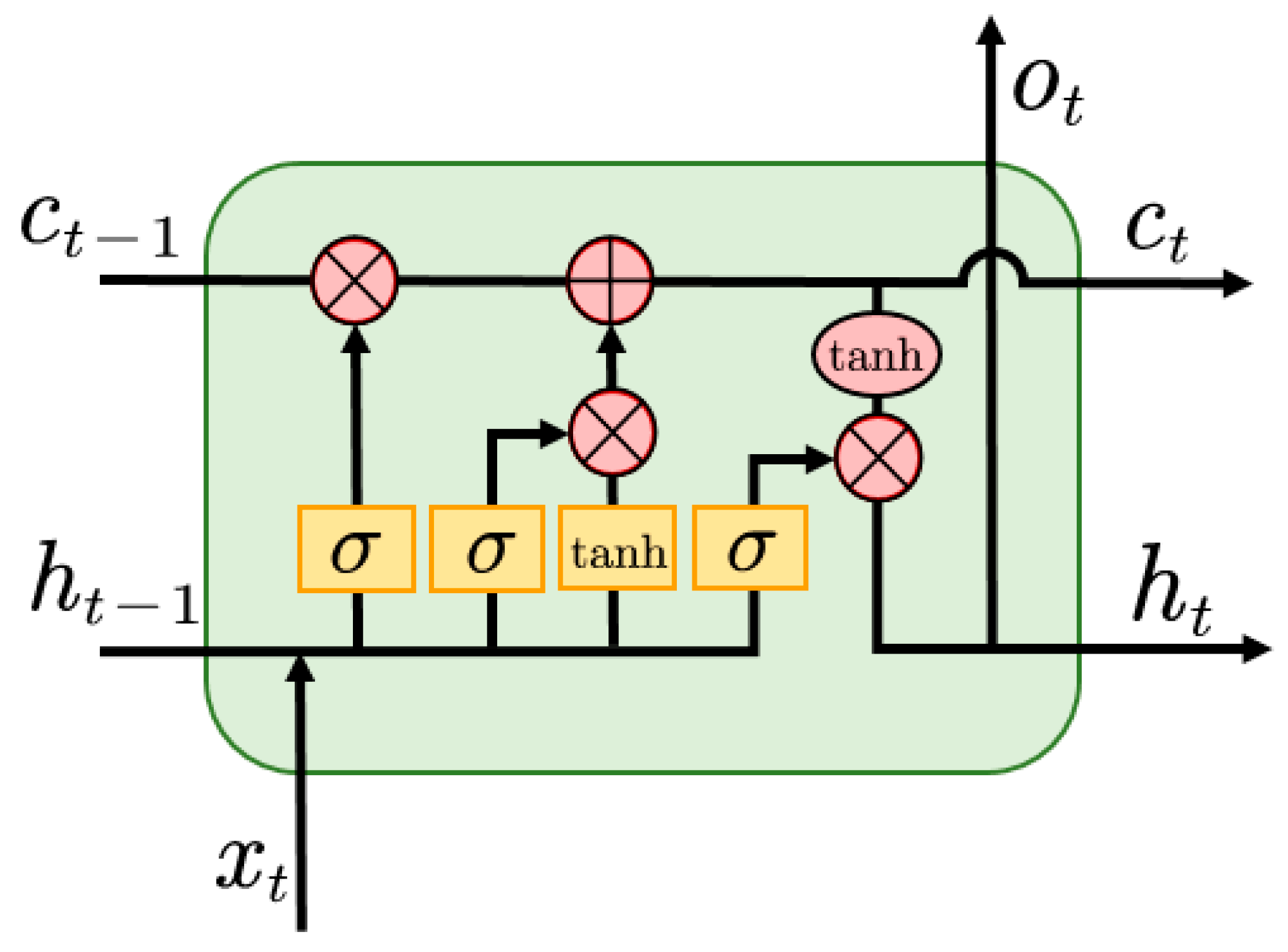
3.1. SwinLSTM Cell

The SwinLSTM Cell, serving as the core spatiotemporal feature extraction module in this model, inherits its concept from the LSTM structure introduced in Section 2.2 and is inspired by ConvLSTM [28].

In SwinLSTM, the hidden state $H_{t-1}$ inherited from the previous time step was first concatenated with the current two-dimensional meteorological data. This combined feature was then input into the Swin Transformer module, as shown in Figure 2, to extract spatial features $F_t$, expressed as follows:

$$F_t=\sigma \left(SwinT\left(LP\left(x_t;H_t\right)\right)\right)$$

(17)

where $LP(.)$ denotes the linear projection layer and $SwinT(.)$ represents the Swin Transformer feature extraction module.

Subsequently, $F_t$ was mapped to the cell state $C_{t+1}$ and the updated hidden state $H_{t+1}$ of the next time step through the forget gate and output gate structures, respectively:

$$C_{t+1}=F_t\circ \left(tanh\right(\mathrm{S}\mathrm{w}\mathrm{i}\mathrm{n}\mathrm{T}\left(LP\left(x_t;H_t\right)\right))+C_t)$$

(18)

$$H_{t+1}=F_t\circ tanh\left(C_{t+1}\right)$$

(19)

where $\circ$ represents the Hadamard product.

3.2. SwinLSTM Block

SwinLSTM Cell is merely a basic structural unit capable of temporal feature transmission. To achieve dynamic spatiotemporal modeling and the prediction of two-dimensional meteorological data distributions, this study designed a SwinLSTM Block comprising multiple SwinLSTM Cells. In addition to the fundamental SwinLSTM Cell, the use of Block incorporates several key modules for processing the data and features input.

Specifically, after the input of two-dimensional meteorological data, $X_t$ was segmented into multiple non-overlapping patches, and the iRPE [29] method was first employed to perform positional encoding on these patches. This introduced relative positional and contextual information to each patch, ensuring that their relative relationships and overall structure were not lost during the partitioning process. Following iRPE encoding, the patches were mapped to a high-dimensional feature space by a Patch Embedding layer with a 1 × 1 convolution kernel. Given that the input and output formats of this meteorological spatiotemporal prediction task remained consistent, this study adopted the encoder–decoder paradigm inspired by the classic U-Net [30] architecture. The features first underwent m downsampling operations, with each downsampling including a SwinLSTM Cell for spatiotemporal feature extraction and a Patch Merging module that combined features of adjacent patches to achieve spatial downsampling. This path corresponded to the hierarchical extraction of spatiotemporal features, capturing representations from fine to coarse granularity. After obtaining the final bottom-level feature representation through downsampling, $m$ upsampling operations followed. Each upsampling operation consisted of a SwinLSTM Cell and a Patch Expansion module. The SwinLSTM Cell is responsible for generating new spatiotemporal feature representations, while the Patch Expansion module expands features in the spatial dimension. This process restored feature resolution gradually, transitioning from abstract semantic features to concrete pixel-level predictions. Finally, after m upsampling operations, the features were mapped back to two-dimensional space through a 1 × 1 convolution layer, outputting the predicted meteorological distribution map ${\widehat{X}}_{t+1}$.

3.3. Loss Function

To simultaneously capture the disparities between predicted and actual meteorological spatiotemporal results, this study proposes a comprehensive loss function to guide model training. This loss function comprises two components: pixel-level regression loss and spatiotemporal gradient loss.

The pixel-level regression loss aims to minimize pixel value differences between predicted and actual values, utilizing a smooth L1 loss function, which is calculated as follows:

$$\begin{array}{c}{\mathcal{L}}_{\mathrm{pixel}}={\displaystyle \frac{1}{MNT}}{\displaystyle \sum _{t=1}^T}{\displaystyle \sum _{i=1}^M}{\displaystyle \sum _{j=1}^N}\mathrm{SmoothL}1\left({\widehat{X}}_{t,i,j}-X_{t,i,j}\right)\end{array}$$

(20)

where T denotes the total prediction time length, M and N represent the horizontal and vertical coordinate ranges of the Kriging-interpolated two-dimensional meteorological distribution, respectively. ${\widehat{X}}_{t,i,j}$ and $X_{t,i,j}$ indicate the predicted and actual values at time t, row i, and column j. $\mathrm{SmoothL}1(·)$ is the smooth L1 loss function, which, compared to traditional norm losses, facilitates stable gradient updates. It is specifically calculated as follows:

$$\begin{array}{c}\mathrm{S}\mathrm{m}\mathrm{o}\mathrm{o}\mathrm{t}\mathrm{h}\mathrm{L}1(x)=\left\{\begin{array}{c}0.5\times x^2, \left|x\right|<1\\ \left|x\right|-0.5, otherwise \end{array}\right.\end{array}$$

(21)

Furthermore, this study introduces spatiotemporal gradient loss, defined as follows:

$$\begin{array}{c}{\mathcal{L}}_{\mathrm{gradient}}={‖{\nabla }_t{\widehat{X}}_{t,i,j}-{\nabla }_t{X}_{t,i,j}‖}_2^2+{‖{\nabla }_i{\widehat{X}}_{t,i,j}-{\nabla }_i{X}_{t,i,j}‖}_2^2+{‖{\nabla }_j{\widehat{X}}_{t,i,j}-{\nabla }_j{X}_{t,i,j}‖}_2^2\end{array}$$

(22)

where ${\nabla }_t$, ${\nabla }_i$, and ${\nabla }_j$ represent gradient calculations in temporal, horizontal, and vertical spatial dimensions, respectively. This loss term penalizes the gradient differences between predicted and actual values in both time and space, facilitating the model’s learning of spatiotemporal evolution patterns.

By linearly combining the aforementioned loss terms, the comprehensive loss function is derived as follows:

$$\begin{array}{c}\mathcal{L}={\lambda }_1{\mathcal{L}}_{\mathrm{pixel}}+{\lambda }_2{\mathcal{L}}_{\mathrm{gradient}}\end{array}$$

(23)

where ${\lambda }_1$ and ${\lambda }_2$ are hyperparameters balancing the two loss terms.

During model training, minimizing this comprehensive loss function yields SwinLSTM with robust spatiotemporal modeling capabilities. The resulting predictions not only closely approximate actual values at the pixel level but also align well with real data in terms of the spatiotemporal evolution structure.

4. Experiments

The model code was developed in a PC environment using Python 3.9 and PyTorch 2.0.1+cu118 deep learning framework, compiled on the Jupyter interactive platform. The hardware configuration included a 13th Gen Intel(R) Core(TM) i5-13600K CPU and an NVIDIA GeForce RTX 3060 GPU.

4.1. Dataset Collection and Preprocessing

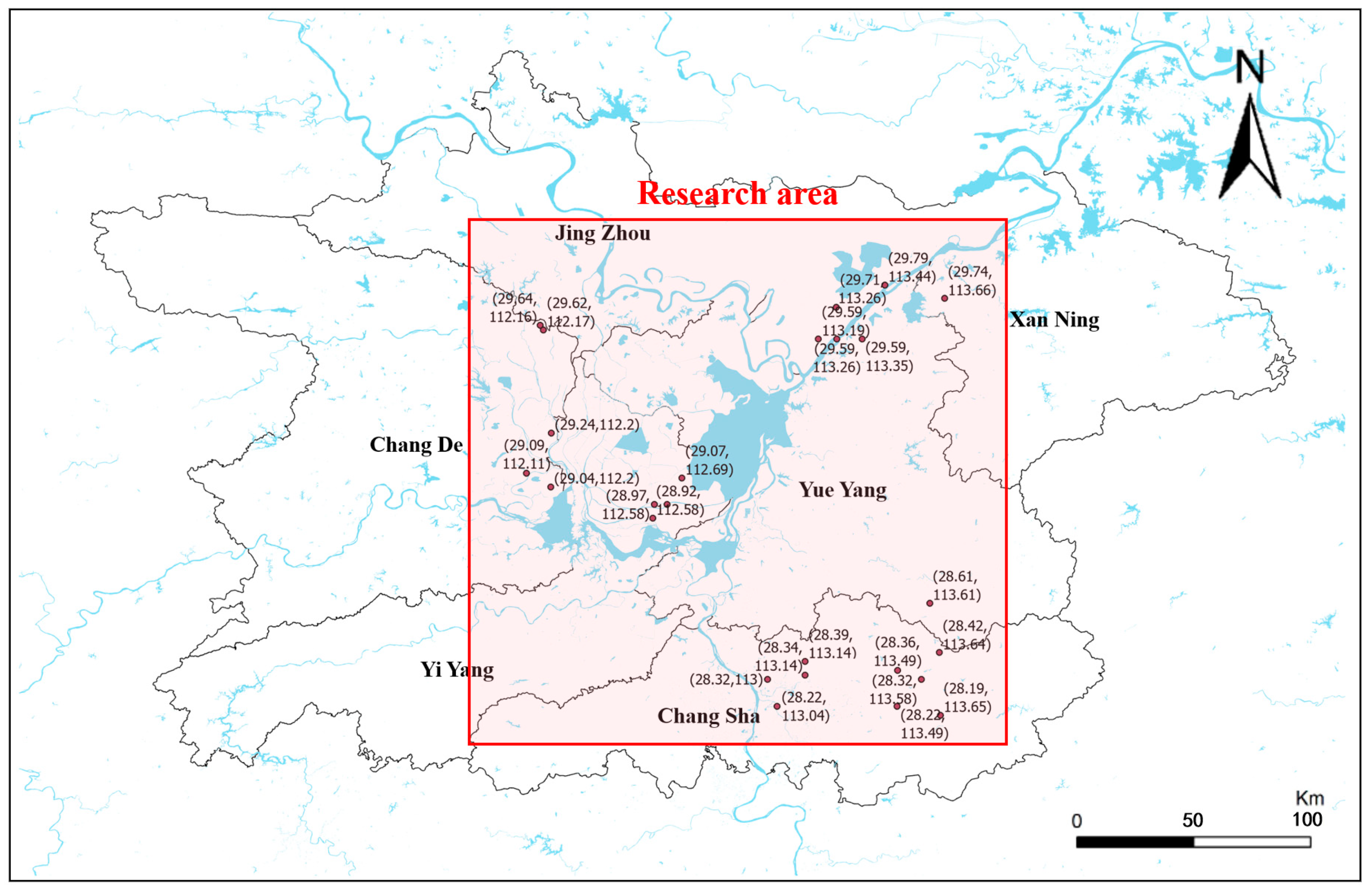
To validate the effectiveness of the proposed research framework, this study collected air quality data from 29 monitoring stations across four cities surrounding China’s Dongting Lake, including Changsha, Yueyang, Changde, and Yiyang, over a three-year period from 1 January 2020 to 31 December 2022. Each monitoring station recorded local air quality indicators at hourly intervals, including the PM2.5, PM10, SO₂ concentration, NO₂ concentration, O₃ concentration, CO concentration, and AQI index. The distribution of the 29 monitoring stations is illustrated in Figure 4, where brown dots represent individual monitoring stations, and blue areas indicate water systems or reservoirs. The meteorological research and prediction area covers the region from 111.60° E to 113.90° E longitude and from 28.00° N to 30.00° N latitude, as indicated by the red area in the figure.

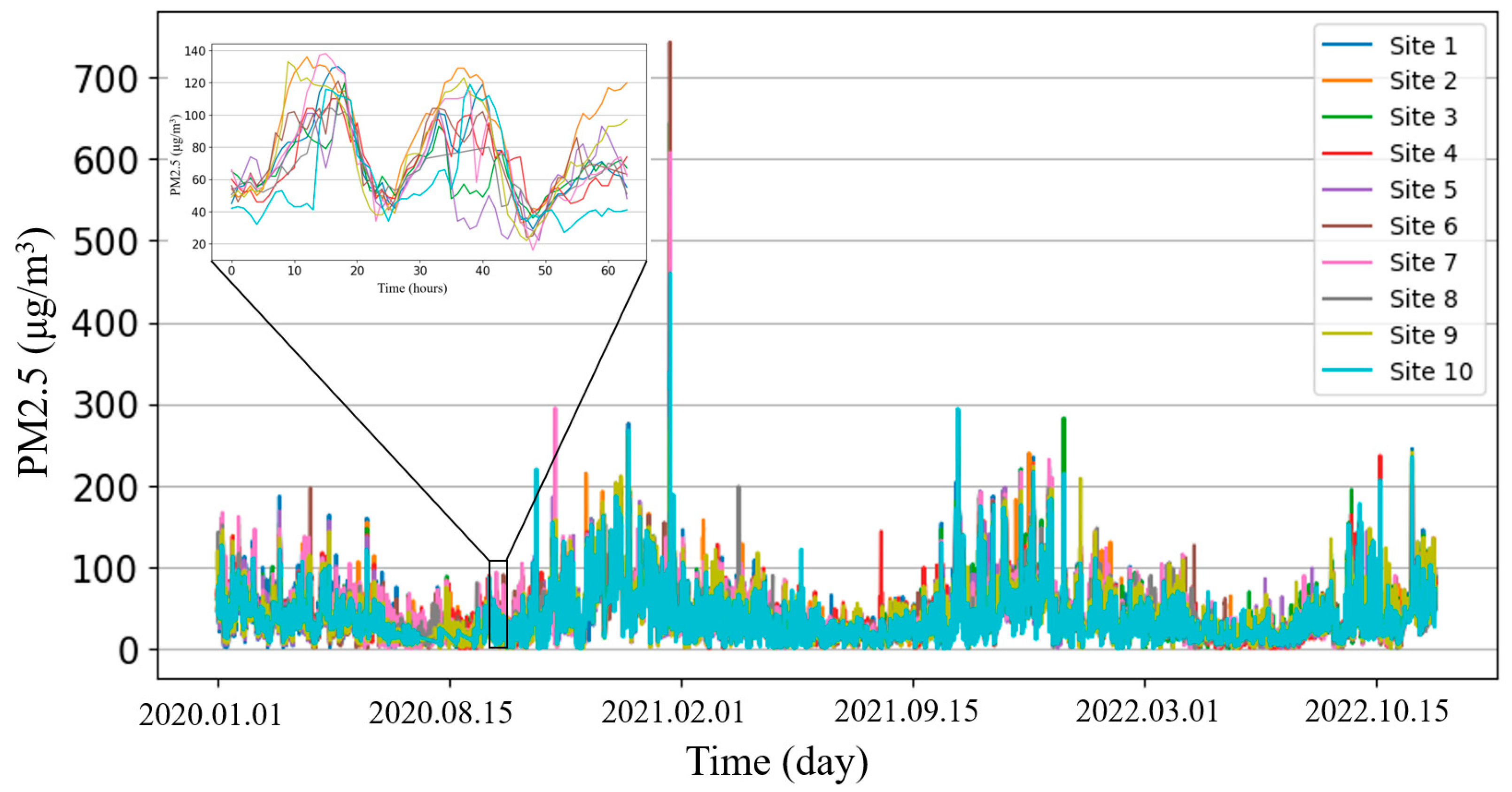
Following data collection, preprocessing was conducted, including the imputation of missing values caused by station malfunctions. The resulting PM2.5 value variation curves collected from multiple stations over the three-year period are shown in Figure 5. Notably, from a long-term macroscopic perspective, PM2.5 variations exhibit an annual cyclical pattern, with higher levels in winter and lower levels in summer. Microscopically, PM2.5 values also demonstrate a daily pattern, with higher levels during the day and lower levels at night. Additionally, it was observed that PM2.5 values from some stations were significantly higher than the group average during certain periods. To mitigate the influence of outliers in the dataset, this experiment employed robust standardization processing. Data scaling based on quartiles was applied to stabilize the data distribution, facilitating the unification of data across different scale ranges while avoiding the impact of extreme values on model training, i.e.:

$$x_i^{*}={\displaystyle \frac{\left(x_i-\mu \right)}{Q_3\left(x\right)-Q_1\left(x\right)}}$$

(24)

where $x_i$ represents the collected raw value, $x_i^{\ast }$ denotes the standardized value, $\mu$ represents the mean of the specific air quality indicator, $Q_1\left(x\right)$ represents the first quartile, and $Q_3\left(x\right)$ represents the third quartile.

4.2. Data Partitioning and Parameter Settings

For the PM2.5 spatiotemporal prediction task, a rolling window modeling approach was adopted. Specifically, for the temporal dimension T, the time series was divided into overlapping sample windows, each containing Δt time steps. The first time steps (a) served as the input feature set $\mathit{Y}=\{{\mathit{X}}_{\mathsf{\Delta }t+1},\dots ,{\mathit{X}}_{\mathsf{\Delta }t+b}\}$, while the subsequent time steps (b) were used as the prediction target $\mathit{Y}=\{{\mathit{X}}_{\mathsf{\Delta }t+1},\dots ,{\mathit{X}}_{\mathsf{\Delta }t+b}\}$. It should be noted that each time step comprised multi-dimensional input features, including not only the air quality indicators to be predicted but also meteorological conditions (temperature, humidity, and wind speed) as auxiliary features, which were aligned with the $\mathit{X}$ features before being input into the model. The dataset was then split into training and testing sets. To satisfy the principle of lagged prediction in the time series models, data from 1 January 2020 to 31 December 2021 (two years) were selected as the training set, while data from 1 January 2022 to 31 December 2022 (one year) were used as the testing set.

In the spatial dimension, Kriging interpolation was applied to the original observational data using monitoring station location information, resulting in 64 × 64 two-dimensional air quality concentration distribution images. Through the aforementioned dataset construction method, the input was defined as a combination of meteorological features and air quality indicators with a feature set step length (a) of 48 h (past two days). The output labels were set as the prediction results for PM2.5 and PM10 indicators at 1, 6, and 24 h ahead to validate the model’s performance across different prediction time spans.

Regarding the model parameters, the number of backbone feature upsampling and downsampling layers m was set to two. The Swin Transformer’s patch size was set to six pixels, with a window size of four patches, an embedding dimension of 64, and four attention heads. For the training configuration, the AdamW optimizer, most compatible with transformer architectures, was employed with a base learning rate of 1 × 10⁻⁴. An exponential decay learning rate strategy based on training steps was adopted, with a decay rate of 0.999 and a step size of one. The total number of training iterations was set to 1000.

4.3. Evaluating Indicator

As air quality spatiotemporal prediction is a regression task, this study implemented three different evaluation metrics: mean absolute error (MAE), Root Mean Square Error (RMSE), and R-squared (R²). The calculation formulas for these metrics are shown in Equations (25), (26), and (27), respectively.

$$MAE={\displaystyle \frac{1}{n}}{\sum }_{i=1}^n\mid y_i-{\widehat{y}}_i\mid$$

(25)

$$MSE=\sqrt{{\displaystyle \frac{1}{n}}{\sum }_{i=1}^n(y_i-{\widehat{y}}_i{)}^2}$$

(26)

$$R^2=1-{\displaystyle \frac{{\sum }_{i=1}^n(y_i-{\widehat{y}}_i{)}^2}{{\sum }_{i=1}^n(y_i-{\overline{y}}_i{)}^2}}$$

(27)

where $n$ represents the sample size, $y_i$ is the true value of the i-th sample, ${\widehat{y}}_i$ is the corresponding predicted value, and ${\overline{y}}_i$ is the mean of all true values. The $R^2$ value ranges from 0 to 1, with values closer to 1 indicating better model predictions and values closer to 0 suggesting poorer predictive performance.

4.4. Result Analysis

Figure 6 presents the experimental results of the proposed SwinLSTM model for the 24 h prediction task compared with the currently mainstream ConvLSTM algorithm.

The results show that the PM2.5 indicator of distribution predicted by the SwinLSTM model more closely aligns with the actual values. This is evident from the mean absolute error percentage (MAEP), where for short-term prediction (t = 1 h), SwinLSTM and ConvLSTM yield errors of 0.60% and 0.95%, respectively. While SwinLSTM leads in terms of accuracy, the difference is not substantial. However, when extending the prediction time step to 24 h, SwinLSTM maintains a high prediction accuracy with an error percentage below 0.9%, while ConvLSTM’s error percentage increases to 2.37%. This demonstrates that the proposed model can better capture spatiotemporal dependencies, thereby improving prediction accuracy.

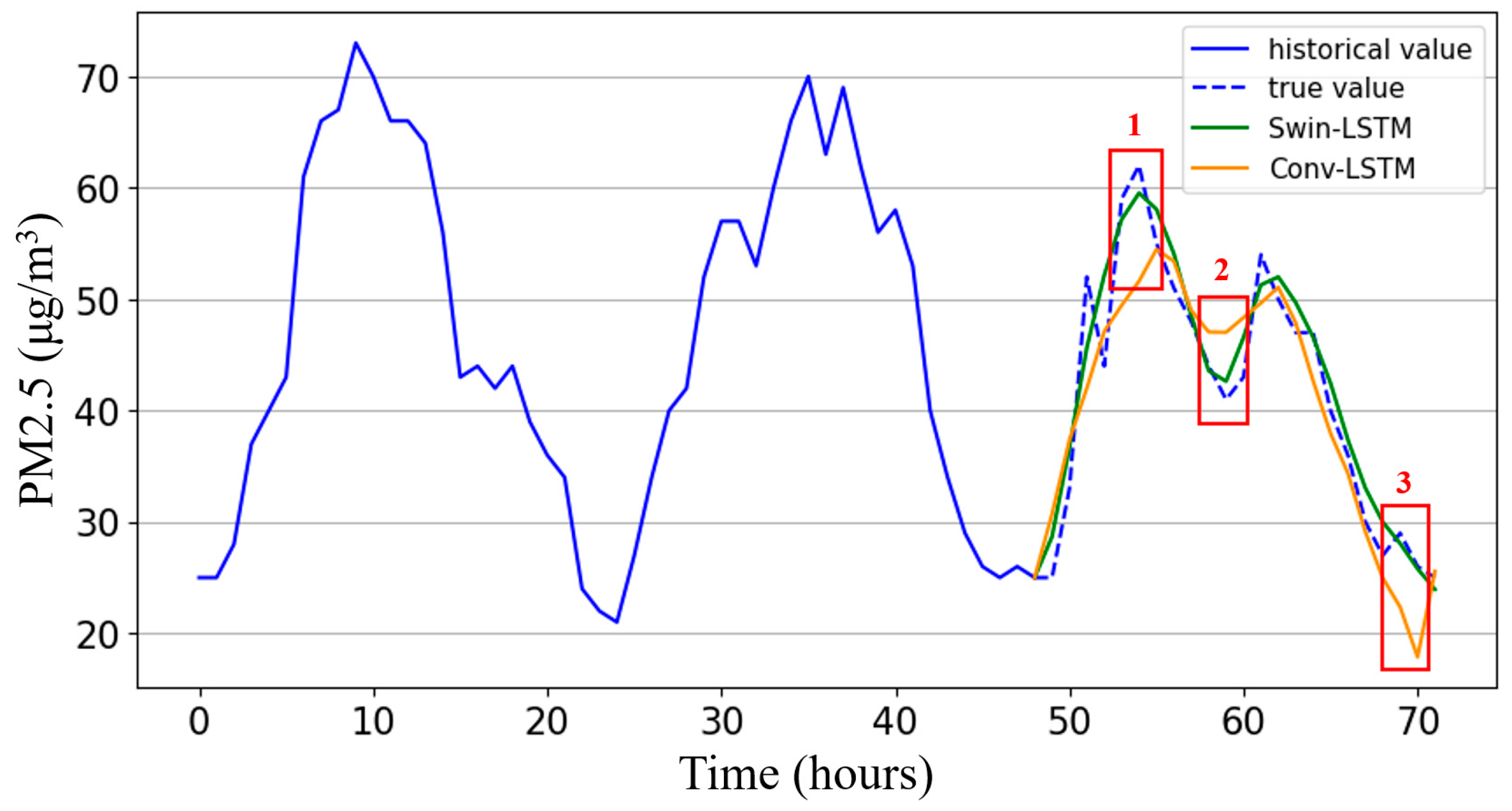
To evaluate the model’s air quality prediction accuracy at fixed locations, samples were taken from the final output PM2.5 indicator spatial distribution map at different times for a single station location. A comparison between the proposed SwinLSTM model and the ConvLSTM model is shown in Figure 7, using Station 1 as a benchmark, with the red box highlighting typical comparison areas.

The SwinLSTM model’s predictions more closely follow the trend of actual observed values, especially when judging daily PM2.5 concentration peaks and troughs. ConvLSTM typically exhibits larger errors at these extreme values, while SwinLSTM maintains higher accuracy. This comprehensively demonstrates that the proposed model, by combining multi-head self-attention mechanisms with LSTM, achieves efficient feature fusion, resulting in more powerful spatial modeling capabilities and the better capture of dynamic patterns in the temporal dimension.

Table 1. PM10 index prediction comparison table.

Method	Model	1 h Forecast			6 h Forecast			24 h Forecast
		MAE	MSE	R2	MAE	MSE	R2	MAE	MSE	R2
Time Series + Kriging	LSTM [31]	0.073	0.295	0.877	0.164	0.390	0.806	0.274	0.436	0.673
	GRU [32]	0.068	0.248	0.898	0.156	0.317	0.821	0.287	0.449	0.668
Kriging + Spatiotemporal	PredRNN [33]	0.026	0.104	0.913	0.085	0.145	0.884	0.149	0.197	0.805
	ConvLSTM [34]	0.010	0.095	0.944	0.037	0.114	0.915	0.089	0.140	0.834
	SwinLSTM	0.009	0.074	0.970	0.015	0.092	0.953	0.028	0.117	0.898

presents comparative results of the SwinLSTM model for PM10 indicators across three different prediction time steps, alongside quantitative comparisons with previously proposed models.

It is evident that the method of first using RNN time series models for single-dimension predictions at each monitoring station, followed by Kriging interpolation to extend predictions to the entire Dongting Lake area, is notably inferior to the approach used in this study. The latter uses Kriging interpolation first, followed by full-area prediction based on two-dimensional meteorological distribution maps. Furthermore, the proposed SwinLSTM exhibited the best performance across all prediction time steps. Compared to ConvLSTM, it showed a 2.75% improvement in the $R^2$ value for 3 h predictions and a 6.47% improvement for 24 h predictions.

4.5. Discussion

The superior performance of the SwinLSTM model can be attributed to several key innovations that address limitations in existing methodologies. Unlike traditional LSTM or GRU models that only capture temporal patterns at individual stations, this study’s approach integrates spatial interpolation with advanced spatiotemporal modeling. The performance gap is particularly evident in medium- to long-term forecasting, where the model maintains high accuracy while pure time series approaches deteriorate rapidly. This improvement stems from SwinLSTM’s ability to model the complex diffusion patterns of pollutants across space. Second, compared to CNN-based architecture like ConvLSTM, the SwinLSTM model demonstrates superior feature extraction capabilities. The shifted window attention mechanism enables both local detail preservation and global context integration, overcoming the fixed receptive field constraints of conventional convolutions. This is particularly important for capturing distant correlations in air quality patterns that may be influenced by regional meteorological phenomena. Third, the hierarchical feature representation in Swin Transformer components allows the model to detect multiscale spatiotemporal dependencies that single-scale models often miss. This is reflected in the 6.47% improvement in R² value for 24 h predictions compared to ConvLSTM, highlighting SwinLSTM’s enhanced capability to maintain prediction accuracy over longer horizons.

The superior long-term prediction capability of SwinLSTM suggests that attention mechanisms more effectively capture persistent spatiotemporal dependencies compared to convolutional approaches. This has significant implications for air quality management, as more accurate 24 h forecasts provide authorities with a crucial lead time for implementing mitigation measures. The model’s ability to capture peak pollution events more accurately than comparison models indicates that the hierarchical representation learning in Swin Transformer components successfully models the complex, non-linear relationships that drive extreme pollution episodes. This capability is particularly valuable for public health applications, as high-concentration episodes pose the greatest health risks.

The performance variations observed also provide guidance for model deployment strategies. For instance, the model could be dynamically configured to emphasize different aspects of its architecture based on the prediction horizon—potentially emphasizing the LSTM components for short-term predictions and the Swin Transformer components for longer-term forecasts. These insights not only validate the theoretical advantages of the proposed SwinLSTM architecture but also offer practical guidance for both model refinement and operational implementation in air quality management systems.

5. Conclusions

This research addresses the crucial environmental monitoring issue of regional air quality spatiotemporal prediction by proposing an innovative deep learning-based method. This method first uses Kriging interpolation to extend multi-dimensional meteorological and pollutant indicators recorded at monitoring stations to two-dimensional distribution images of the entire region. It then employs the proposed SwinLSTM model to predict future regional air quality in both spatial and temporal dimensions.

The experimental results from the Dongting Lake area in China demonstrate that the proposed SwinLSTM model not only achieves excellent results in short-term PM2.5 and PM10 prediction tasks, significantly outperforming the current mainstream ConvLSTM model but also shows more pronounced advantages in medium- to long-term prediction tasks. This proves that the proposed model can better capture the spatiotemporal correlations and evolution patterns of regional air quality.

Despite the promising results, several limitations of this study should be acknowledged. Data availability constraints restricted the analysis to a three-year period and specific pollutants; a longer time series and additional pollutants could enhance the model’s robustness. The model’s performance is dependent on the specific geographical and meteorological conditions of the Dongting Lake region, potentially limiting direct transferability to regions with substantially different characteristics without retraining or adaptation. The computational resources required for the SwinLSTM architecture may present implementation challenges for real-time prediction systems with limited processing capabilities.

Future work will explore more comprehensive and efficient spatiotemporal feature fusion methods, such as considering geographical factors like terrain, lakes, and altitude, to enable the model to better capture geographical conditions affecting air quality dispersion. Cross-attention mechanisms for multimodal fusion will be used to model spatiotemporal features. Additionally, the incorporation of forecast data from numerical weather models into input features will be attempted to further improve prediction fidelity. Furthermore, empirical studies on meteorological predictions will be conducted over larger regional scales, and predictions for more meteorological indicators will be made. This will provide technical support for formulating more comprehensive environmental control policies, demonstrating important theoretical value and practical significance across a wider range of fields.