Spatiotemporal Analysis and Prediction of Avian Migration Under Climate Change

Abstract

Frequent bird strikes during peak migration periods pose a significant risk to aviation safety. Existing prevention methods rely on static historical patterns and lack the ability to adapt to real-time changes. Short-term meteorological fluctuations are crucial in shaping bird migration behavior, influencing both its timing and intensity. Climate change increases the variability of these factors, making predictions more difficult. Simple models may describe migration patterns under stable conditions but struggle to capture the complexity introduced by climate-driven fluctuations. To address this, we propose a model that integrates convolutional neural networks (CNNs), long short-term memory (LSTM) networks, and an attention mechanism, achieving prediction accuracy consistently above 0.9. CNN extracts features, LSTM captures temporal dependencies, and attention assigns weights to important features. Unlike traditional statistical methods, this model transitions from traditional heuristic approaches to data-driven quantitative forecasting, offering insights into migration intensity while accounting for meteorological fluctuations influenced by climate change. Ablation experiments showed that removing the attention mechanism, CNN module, and both components reduced the average prediction accuracy by 3.93%, 8.47%, and 10.96%, respectively. These results demonstrate that bird migration predominantly occurs at night and is significantly influenced by radiation levels and wind conditions. This research incorporates meteorological variability into predictive modeling to develop data-driven strategies for enhancing aviation safety. Additionally, it addresses environmental challenges and promotes sustainable practices by optimizing flight schedules to reduce bird strikes, improve fuel efficiency, and minimize emissions. This approach also contributes to ecological conservation and supports sustainability goals.

1. Introduction

A bird strike is an aviation safety incident caused by a collision with a bird during takeoff, cruising, or landing [1]. During spring and autumn migrations, billions of birds travel between breeding and non-breeding areas [2], significantly increasing the likelihood of collisions with aircraft and leading to bird strike events [3,4]. It is estimated that bird strikes cost the global commercial aviation industry over USD 1.2 billion annually [5]. These incidents not only cause substantial economic losses but also pose a direct threat to the safety of flight crews and passengers.

Bird migration is a complex ecological phenomenon, involving intricate relationships with meteorological factors. Understanding and predicting migratory patterns requires considering various meteorological factors and their interactions. Wind conditions are crucial in determining optimal flight speed, altitude, and migration routes for birds [6]. The effect of temperature on migration is primarily reflected in the timing of departures from wintering grounds and arrivals at breeding grounds. With global warming, birds are migrating earlier, which impacts resource availability at breeding sites and, consequently, population abundance and future migration intensity [7]. Changes in precipitation impact food resource availability, prompting birds to adjust their migration timing accordingly [8]. Additionally, humidity helps regulate protein metabolism and maintain water balance during migration [9]. The duration and intensity of sunlight control the circadian rhythm in birds, which shifts from daytime activity to nocturnal migration during the migration season, leading to increased nocturnal activity [10]. However, the effects of different meteorological factors on bird migration are often interrelated [11]. Birds take multiple meteorological factors into account during migration to optimize their survival and reproductive success.

Advancements in weather radar technology have enabled ornithologists to record and measure bird movements that were previously difficult to observe. Cohen et al. [12] utilized weather radar, in conjunction with geographic information data, to analyze the spatial distribution of birds during their spring and autumn migrations, addressing the problem of siting wind energy facilities. Similarly, Elmore et al. [13] correlated daily bird collision data in urban areas to effectively reduce the risk of collisions between birds and artificial structures. These studies present a new approach to constructing quantitative models that relate bird migration intensity to various meteorological factors, highlighting the potential of combining weather radar data with conventional meteorological data. However, traditional data processing methods face challenges in efficiently handling such large-scale data. The advantages of machine learning technology in processing big data related to bird activity have gradually led to its widespread adoption. For instance, using advanced machine learning techniques, Pancerasa et al. [14] developed an automated data preprocessing program that filtered approximately 40,000 geolocation data points from 108 swallow migration trajectories, with results consistent with those manually processed by experts. The Kabasakal team overcame the limitations of traditional methods by using convolutional neural networks to count birds from photographs taken in their natural environment [7]. Manual counting methods are often costly, time-consuming, and susceptible to observer bias and environmental factors [15]. Similarly, Lostanlen’s team combined multiple machine learning modules to analyze 6672 h of recorded bird audio data, achieving accurate species-level classification [16]. Machine learning technology enables the development of models to quantify the impact of various meteorological factors on bird migration intensity, providing a scientific basis for bird strike risk assessment and prediction.

The primary challenge in bird strike prevention is the limited understanding of bird activity and migration patterns. Traditional bird prediction methods rely mainly on simple statistical analyses of historical observation data, without adequately considering real-time environmental and dynamic factors. Additionally, large-scale monitoring and analysis techniques for bird migration remain underdeveloped, making it difficult to understand long-term dynamic changes in migration patterns and environmental influences. These limitations hinder a comprehensive assessment of bird strike risks and the formulation of effective long-term prevention strategies. Previous studies have often focused on the impact of one or a few meteorological factors on bird migration, neglecting the combined effects of multiple factors. Weather radar data have not fully utilized the potential of integrating meteorological data to assess bird activity or to identify and quantify the key meteorological factors influencing bird migration. To improve the prediction of bird strike risks and better understand the primary meteorological drivers and mechanisms affecting bird migration, this paper employs machine learning technology to explore the complex quantitative relationships between meteorological factors and bird migration intensity along the central China migration route. By integrating weather radar and conventional meteorological data, a predictive model for bird migration intensity is established. By accurately predicting migration paths and peak activity times, we can proactively identify high-density bird areas and implement preventive measures, such as adjusting flight routes or schedules. This approach not only minimizes bird strikes but also reduces resource wastage, such as aircraft repairs and flight delays. Consequently, it helps lower carbon emissions, contributing to more environmentally friendly and sustainable aviation operations. Additionally, it promotes interdisciplinary research between ecology and meteorology, fostering the development of related fields.

2. Materials and Methods

The relationship between meteorological factors and bird migration is complex and nonlinear, which makes accurate modeling using traditional statistical methods challenging. Machine learning models, however, can effectively capture this complexity. These models possess strong feature selection and dimensionality reduction capabilities, enabling them to identify the most relevant features for migration intensity from a large set of meteorological factors.

2.1. Model Architecture

2.1.1. Tree Model

Tree models are a class of machine learning algorithms that use a tree structure to recursively divide datasets into different subsets, forming a tree-like structure to perform prediction tasks [17]. In this study, the tree model is based on Gradient Boosting Decision Tree (GBDT), including implementations such as EXtreme Gradient Boosting (XGBoost) [18], Light Gradient Boosting Machine (LightGBM) [19], and Categorical Boosting (CatBoost) [20].

(1)

XGBoost

The basic idea of XGBoost is to iteratively improve the accuracy of predictions by adding new weak learners to correct the errors made in previous rounds [21]. The optimization objective function is shown below:

$$L(\theta )={\sum }_{i=1}^n l\left(y_i,{\hat{y}}_i\right)+{\sum }_{k=1}^K \Omega \left(f_k\right)$$

(1)

where $L(\theta )$ is the objective function, $y_i$ is the true value, ${\hat{y}}_i$ is the predicted value, $l$ is the loss function, $\Omega$ is the regularization term, and $f_k$ represents the model of the $k$th tree.

XGBoost optimizes the objective function iteratively using an additive model, as shown in Equation (2).

$${\hat{y}}_i={\sum }_{k=1}^K f_k\left(x_i\right), f_k\in F$$

(2)

where $F$ is the space for all possible trees.

The optimization goal for each step is to minimize the residuals, as follows:

$$r_i^m=-{\displaystyle \frac{\partial L(y_i,{\hat{y}}_i^{m-1})}{\partial {\hat{y}}_i^{m-1}}}$$

(3)

In each iteration, the new tree $f_m$ optimizes the objective function by fitting the current residuals $r_i^m$. The final model is a weighted sum of multiple trees.

(2)

LightGBM

LightGBM makes predictions by constructing multiple decision trees, aiming to minimize the loss function [22]. The basic optimization objective can be expressed as follows:

$$L\left(\theta \right)={\sum }_{i=1}^n l\left(y_i,{\hat{y}}_i\right)+{\sum }_{k=1}^K \Omega \left(f_k\right)$$

(4)

where $L(\theta )$ is the objective function, $y_i$ is the true value, ${\hat{y}}_i$ is the predicted value, $l$ is the loss function, $\Omega$ is the regularization term, and $f_k$ represents the model of the $k$th tree.

LightGBM uses a segmented histogram algorithm to accelerate the process of building decision trees. The basic idea is to divide continuous feature values into discrete intervals, thereby reducing computational complexity. The specific calculation method is described as follows:

Assuming the dataset is ${\left\{\left(x_i,y_i\right)\right\}}_{i=1}^n$ where $x_i$ is the eigenvector and $y_i$ is the target value. The goal of LightGBM at the mth round iteration is to minimize the following loss functions:

$$L_m={\sum }_{i=1}^n l\left(y_i,{\hat{y}}_i^{(m-1)}+f_m\left(x_i\right)\right)+\Omega \left(f_m\right)$$

(5)

where ${\hat{y}}_i^{(m-1)}$ is the prediction value of the previous $m-1$ rounds, and $f_m$ is the prediction function of the $m$th tree. In each iteration, LightGBM selects the best split point through a greedy algorithm to maximize the decline of the loss function.

(3)

CatBoost

CatBoost makes predictions by constructing multiple decision trees [23], with the optimization objective function expressed as follows:

$$L\left(\theta \right)={\sum }_{i=1}^n l\left(y_i,{\hat{y}}_i\right)+{\sum }_{k=1}^K \Omega \left(f_k\right)$$

(6)

where $L(\theta )$ is the objective function, $y_i$ is the true value, ${\hat{y}}_i$ is the predicted value, $l$ is the loss function, $\Omega$ is the regularization term, and $f_k$ represents the model of the $k$th tree.

Similarly to LightGBM, CatBoost constructs a decision tree in each iteration by selecting the optimal split point to maximize the reduction in the objective function.

2.1.2. Neural Networks

Neural networks are a class of machine learning models inspired by the principles of biological nervous systems. Their structure typically consists of an input layer, several hidden layers, and an output layer [24]. Each layer contains multiple neurons connected by weights. Using the backpropagation algorithm, the neural network can iteratively adjust the weights layer by layer to minimize prediction errors, enabling the fitting and prediction of complex functions.

(1)

Long Short-Term Memory (LSTM)

The core of LSTM lies in its memory unit and three gating mechanisms: the input gate, the forget gate, and the output gate [25]. The calculation process for each LSTM cell at a given time step is as follows:

Forget Gate: Determines how much of the past information should be forgotten, as shown in Equation (7).

$$f_t=\sigma \left(W_f\cdot \left[h_{t-1},x_t\right]+b_f\right)$$

(7)

Input Gate: Determines how much new information should be added to the memory, as described in Equations (8) and (9).

$$i_t=\sigma \left(W_i\cdot \left[h_{t-1},x_t\right]+b_i\right)$$

(8)

$${\tilde{C}}_t=\tanh \left(W_C\cdot \left[h_{t-1},x_t\right]+b_C\right)$$

(9)

Update Memory Cell: The memory cell is updated by combining the outputs of the forget gate and the input gate, as described in Equation (10).

$$C_t=f_t\ast C_{t-1}+i_t\ast {\tilde{C}}_t$$

(10)

Output Gate: Determines the amount of information to be output from the memory cell, as described in Equations (11) and (12).

$$o_t=\sigma \left(W_o\cdot \left[h_{t-1},x_t\right]+b_o\right)$$

(11)

$$h_t=o_t\ast \tanh \left(C_t\right)$$

(12)

where $\sigma$ is the Sigmoid function, $\mathrm{t}\mathrm{a}\mathrm{n}\mathrm{h}$ is the hyperbolic tangent function, $W$ and $b$ is model parameters, $h_t$ is the output of the current time step, and $C_t$ is the memory unit state of the current time step.

(2)

Convolutional Neural Networks (CNNs)

CNNs are primarily used to process data with grid-like structures, such as images and time series data. The core idea is to extract local features from the input data using the convolutional layer and reduce dimensionality through the pooling layer, thereby retaining important information while decreasing computational complexity [26].

The operation of the convolutional layer can be expressed by the following formula:

$$y_{i,j,k}={\sum }_m {\sum }_n x_{i+m,j+n}\cdot w_{m,n,k}+b_k$$

(13)

where $y_{i,j,k}$ is the value of the $k$th channel of the convolution output at position $(i,j)$, $x_{i+m,j+n}$ is the subregion of the input data, $w_{m,n,k}$ is the weight of the convolution kernel, and $b_k$ is the bias term.

2.1.3. Attention Mechanisms

The attention mechanism allows the model to focus on the most important information by assigning different weights to each element in the input sequence. It has demonstrated powerful performance in tasks such as machine translation and natural language processing. The core idea is to calculate the importance of each element in the input sequence and perform a weighted sum of the inputs based on these weights [27]. The calculation process of the attention mechanism is as follows:

Calculate Attention Weights: For an input sequence $x=\left[x_1,x_2,\dots ,x_n\right]$, compute the attention score for each element:

$$e_{ij}=f\left(x_i,h_j\right)$$

(14)

where $f$ is a learnable function, such as a dot product or feedforward neural network.

Normalize Attention Weights: Convert the attention scores into a probability distribution using the softmax function, as shown in Equation (15).

$${\alpha }_{ij}={\displaystyle \frac{\exp \left(e_{ij}\right)}{{\sum }_k \exp \left(e_{ik}\right)}}$$

(15)

Weighted Summing: The inputs are weighted and summed based on the normalized attention weights, as described in Equation (16), resulting in a new representation.

$$z_j={\sum }_i {\alpha }_{ij}{x}_i$$

(16)

2.2. Data

2.2.1. Data Sources

Weather radar data were acquired using the Doppler Weather Radar (CINRAD-SAD). The radar data analysis was conducted using the bioRad software package (version 0.8.1), a tool specifically designed for analyzing and visualizing weather radar data in biological research [28]. The bird migration data in this study were primarily characterized by the Migration Traffic Rate (MTR), which represents the number of birds passing through a 1 km virtual transect perpendicular to the migration direction per hour. MTR combines bird distribution density and flight speed to indicate the number of birds passing through a specific area each hour, expressed in units of birds per kilometer per hour [29]. Conventional meteorological data were obtained from the Xihe Energy Meteorological Big Data Platform, including datasets of various meteorological elements such as temperature, precipitation, wind, and solar radiation, as shown in

Table 1. Meteorological factors and identifiers.

Meteorological Factors	Unit
Temperature	°C
Humidity	%
Atmospheric pressure	hPa
Precipitation	mm/h
Meridional wind	m/s
Zonal wind	m/s
Surface wind speed	m/s
Wind direction	degree
Global horizontal irradiance	W/m2
Direct normal irradiance	W/m2
Diffuse horizontal irradiance	W/m2

. The specific definitions of these elements are provided in

Table A1. Meteorological factors and definitions.

Meteorological Factors	Definition
Temperature	Temperature in a shelter located approximately 1.5–2 m above ground level
Humidity	Air humidity at approximately 1.25–2 m above ground level
Atmospheric pressure	Atmospheric pressure of the region
Precipitation	Amount of liquid or solid (after melting) water falling from the sky and reaching the ground
Meridional wind	Meridional component of wind at approximately 10 m above ground (positive for southerly winds)
Zonal wind	Zonal component of wind at approximately 10 m above ground (positive for westerly winds)
Surface wind speed	Wind speed at approximately 10 m above ground level
Wind direction	The direction of the wind origin, measured from true north (0°) clockwise
Global Horizontal Irradiance	Total solar radiation received per unit area on the Earth’s horizontal surface
Direct Normal Irradiance	Direct radiation incident perpendicular to the plane directly from the Sun’s rays
Diffuse Horizontal Irradiance	Radiation scattered by the atmosphere (clouds, air particles) before reaching the Earth’s surface

in Appendix A.

2.2.2. Scope of the Study

In China, bird migration routes are primarily divided into three main pathways: eastern, central, and western [30]. The central route, which passes through the provinces of Hebei, Henan, Hubei, and Hunan, is a vital corridor connecting northern and southern China. It also forms part of the East Asian–Australasian migration route [31], playing a key role in the breeding and wintering of many bird populations.

Due to challenges in obtaining weather radar data, this study focuses on the spring and autumn migration seasons of 2023. The selected research locations, from north to south, are Zhangjiakou, Shijiazhuang, Zhengzhou, Yichang, and Changsha, chosen based on geographical coverage and data availability. However, due to poor-quality radar data and significant gaps during the autumn migration in Changsha and its surrounding areas, a scientific and effective analysis could not be conducted there. Consequently, the study cities for the autumn migration are limited to Zhangjiakou, Shijiazhuang, Zhengzhou, and Yichang. The selected cities are strategically located along key migration corridors in central China, connecting northern breeding grounds to southern wintering areas. Spanning latitudes from 41° N (Zhangjiakou) to 28° N (Changsha), these cities offer a comprehensive representation of the ecological and geographical conditions that influence bird migration. This selection allows for a thorough evaluation of the model’s ability to handle diverse migration patterns across different regions. Additionally, the cities encompass a wide range of climate types, including temperate continental (Zhangjiakou), temperate monsoon (Shijiazhuang and Zhengzhou), and subtropical humid (Yichang and Changsha) climates. This climate diversity enables the assessment of the model’s sensitivity to various meteorological factors, such as temperature, humidity, wind, and radiation, which vary significantly across regions. By including cities with diverse climatic and ecological conditions, we ensure the model is validated across a broad spectrum of environments, enhancing its robustness and generalizability to regions with varying radar coverage and weather conditions.

2.2.3. Data Preprocessing

To ensure the accuracy of bird migration data, several thresholds were applied to filter out noise and interference [28]. A Raw Reflectivity threshold of −5 dBZ excluded weak signals, while a Bird Reflectivity threshold of 15 dBZ removed precipitation-related echoes. Speed consistency was maintained by filtering out signals with a standard deviation of velocity greater than 1 m/s, as these typically indicate non-avian targets. Additionally, radar data were cross-validated with airport observation reports to ensure time and spatial alignment with actual bird movements. These criteria effectively distinguish valid bird migration signals from common interferences, providing a reliable dataset. To address inconsistencies in data format and accuracy across different sources, data processing software was developed using Python (version 3.11). Researchers interested in accessing this software can contact the author via email. This software standardizes data formats, ensures accuracy, automates data processing, and provides a reliable foundation for predicting bird migration intensity using conventional meteorological data.

To complete the missing MTR values for subsequent analysis, interpolation was required. Traditional interpolation methods typically consider only one or a few dimensions, limiting their ability to capture complex interactions among multiple features. Additionally, these methods often rely solely on relationships between interpolation points and neighboring data, overlooking the dynamic characteristics of time series data. To overcome these limitations, three Gradient Boosting Decision Tree (GBDT)-based models—XGBoost, LightGBM, and CatBoost—were employed to predict the MTR values by integrating meteorological and temporal features. We selected GBDT models for their ability to handle missing data without complex augmentation, making them ideal for small, incomplete time series. Their robustness in imputing missing values through ensemble learning ensures reliable results. Additionally, GBDT models are highly interpretable, allowing us to understand how features like temperature or wind speed influence bird migration predictions, which is crucial for applications like bird strike prevention. Lastly, their computational efficiency allows for quick model evaluation, making GBDT a practical choice compared to more resource-intensive deep learning methods. The MTR value exhibits clear periodicity and trends, making the incorporation of time features beneficial for capturing its temporal characteristics and improving interpolation accuracy. However, tree-based models are not inherently designed for time series data and cannot be processed directly. By applying feature engineering and one-hot encoding, we integrate temporal features into tree models. One-hot encoding is a widely used data preprocessing technique that converts categorical variables into numerical features, enabling the model to effectively utilize them [32]. Given the strong monthly and diurnal periodicity of bird migration intensity, the month and hour of the day were selected as temporal features, as they are crucial for predicting migration intensity.

The dataset was split into training, test, and validation sets in a 70:15:15 ratio. For hyperparameter tuning during interpolation, traditional grid search and random search methods were not used. Instead, the Optuna library in Python was employed, utilizing a Bayesian optimization algorithm to enhance the efficiency of hyperparameter searching. The optimal hyperparameters and evaluation metric scores for the different models are provided in

Table A3. The optimal parameters and the highest R² score achieved in the XGBoost model.

Parameters	Zhangjiakou	Shijiazhuang	Zhengzhou	Yichang	Changsha
max_depth	12	7	3	8	18
n_estimators	800	1700	1500	1050	1250
subsample	0.01	0.11	0.0699	0.04	0.05
colsample_bytree	6	2	7	5	4
learning_rate	0.0028	0.5402	0.0569	8.17 × 10−5	0.1861
min_child_weight	0.0090	0.0003	7.3166	0.2255	0.0026
reg_alpha	0.8808	0.5778	0.7268	0.7579	0.6273
reg_lambda	0.9599	0.9872	0.8018	0.6647	0.7408
R2	0.9239	0.9276	0.9262	0.8951	0.8305

,

Table A4. The optimal parameters and the highest R² score achieved in the LightGBM model.

Parameters	Zhangjiakou	Shijiazhuang	Zhengzhou	Yichang	Changsha
max_depth	7	17	3	20	14
n_estimators	1250	1500	1200	400	1300
learning_rate	0.13	0.26	0.05	0.04	0.03
num_leaves	77	133	83	69	95
min_child_samples	26	16	11	7	3
min_child_weight	9	10	3	6	1
subsample	0.5861	0.9157	0.9479	0.9894	0.9649
colsample_bytree	0.7609	0.9105	0.5770	0.6908	0.5449
reg_lambda	0.7399	0.0001	0.0563	0.0001	3.8342
reg_alpha	0.0009	0.0006	0.0005	2.8830	0.5515
R2	0.8467	0.9544	0.9501	0.9205	0.8717

and

Table A5. The optimal parameters and the highest R² score achieved in the Catboost model.

Parameters	Zhangjiakou	Shijiazhuang	Zhengzhou	Yichang	Changsha
depth	7	9	6	9	9
iterations	1300	1900	2000	1800	1000
learning_rate	0.2	0.2299	0.2	0.25	0.2
l2_leaf_reg	9	9	14	11	9
random_strength	18	3	16	13	41
bagging_temperature	0	0	10	5	8
colsample_bylevel	0.5544	0.8203	0.8524	0.7484	0.6662
R2	0.8779	0.8842	0.9658	0.8746	0.8142

in Appendix B.

3. Results and Discussion

3.1. Model Interpretation Tools

Complex models often exhibit a black-box nature, making their results difficult to interpret [33]. To address this, the study employed the SHapley Additive exPlanations (SHAP) method [34]. Based on Shapley values from game theory, the SHAP method quantifies feature importance by calculating the marginal contribution of each feature to the prediction outcome. The underlying principles are outlined in Equation (17). The SHAP value was used to precisely quantify the effects of meteorological factors and time on bird migration intensity, enabling the identification of key drivers.

$${\varphi }_i={\sum }_{S\subseteq N\setminus \left\{i\right\}} {\displaystyle \frac{\left|S\right|!\left(\right|N|-|S|-1)!}{\left|N\right|!}}[v(S\cup \{i\})-v(S)]$$

(17)

where ${\varphi }_i$ is the Shapley value of the feature $i$, $S$ is the feature subset, $N$ is the total feature set, and $v\left(S\right)$ is the model output corresponding to the feature subset $S$.

3.2. Analysis of the Importance of Spring Migration Characteristics

3.2.1. Temporal Feature Importance Analysis for Spring

To identify the peak period of bird migration, we calculated the mean absolute SHAP value of the temporal features. A higher value indicates that the feature contributes more significantly to the prediction results.

Meteorological and temporal features interact during the migration process, creating a complex migration pattern. As shown in Figure 1, the following patterns emerged: (a) Regarding monthly variation, May had the most significant influence on migration intensity in all cities, indicating that late spring is the peak period for migration as birds strive to reach their breeding grounds before summer. Some cities, such as Zhengzhou, Yichang, and Changsha, also exhibited strong migration activity in early and mid-spring (March and April), likely due to warmer temperatures that favor early migration, with mid-spring serving as a key migration stage. This trend aligns with the biological clock and climate adaptation strategies of bird migration. (b) In terms of diurnal variation, the night and early morning hours (e.g., 20:00, 21:00, 23:00, 00:00, 01:00) had a significant impact on migration intensity. Nocturnal migration enhances the success rate of migrations by reducing energy expenditure, avoiding predators, and taking advantage of more stable airflow and celestial navigation while also minimizing water loss through evaporation.

Helm examined the physiological and behavioral mechanisms of bird migration, focusing on circadian and circannual rhythms [35]. However, it did not provide specific data on the activity intensity and timing of birds during migration. In contrast, our study quantifies the relative contribution of bird activity across different months and hours, offering a more precise reference for studying migration behavior. Liu used bioacoustic monitoring to capture the flight calls of migrating birds, providing real-time activity data [36]. However, compared to radar data, its temporal precision and quantification are limited and may be affected by environmental noise and equipment positioning.

3.2.2. Importance Analysis of Meteorological Characteristics for Spring

To quantitatively analyze the contribution of meteorological factors to the predicted MTR values, a SHAP value scatter plot was used for the interpretation [37]. In the scatter plot, red dots indicate a positive contribution, meaning that higher feature values correspond to larger SHAP values and increased migration intensity. Conversely, blue dots indicate a negative contribution, where higher feature values correspond to smaller SHAP values and reduced migration intensity. The density and distribution of the feature scatter points reflect their importance, with features that are more widely spread and denser contributing more significantly to the model’s predictions. The SHAP value scatter plot is organized by feature importance, with the most important features appearing at the top.

Compared to existing studies [38,39,40,41], our research offers significant advantages in analyzing the relationship between climate factors and bird migration. We focus on the interactions between these factors and their combined influence on migration decisions. Additionally, our study quantitatively measures the impact of climate factors on MTR, providing concrete data support. In contrast, existing studies either focus on individual factors or lack quantitative analysis, overlooking the complex interactions between climate variables.

As shown in Figure 2a–c, Zhangjiakou, Shijiazhuang, and Zhengzhou are located in the temperate and warm temperate monsoon climate zones of northern and central China, where spring conditions include dry weather and abundant sunshine, creating similar migration environments. Among the meteorological factors, diffuse horizontal irradiance had the most significant negative effect on migration intensity, with high radiation levels inhibiting migratory activity. This suggests that birds prefer to migrate under low radiation conditions or at night, possibly because high scattered radiation disperses light, making navigation more difficult. Surface wind speed and direction also had a prominent influence. Southerly winds (meridional wind) in Zhangjiakou and Zhengzhou supported the northward migration of birds, while westerly winds (zonal wind) positively affected migration in Shijiazhuang. Favorable temperatures and moderate wind speeds promoted migration, but extreme atmospheric pressure (either high or low) and extreme wind speeds inhibited migratory activity. Additionally, humidity and precipitation negatively impacted bird migration in these cities, with higher humidity and precipitation increasing flight resistance and causing birds to halt migration.

As shown in Figure 2d,e, Yichang and Changsha are located in southern China and experience a subtropical monsoon climate characterized by wet and rainy springs, which differ markedly from the conditions in northern cities. In Yichang, diffuse horizontal irradiance and direct normal irradiance continue to be major factors inhibiting migration, while wind direction plays a more significant role, with variable wind patterns caused by complex terrain posing challenges for bird navigation. Additionally, fluctuations in atmospheric pressure and humidity greatly influence migration intensity, with low pressure and high humidity conditions leading to a significant reduction in migratory activity. In contrast, humidity in Changsha has a positive effect on migration intensity, likely because Changsha serves as an important starting point for birds migrating northward. High humidity often indicates abundant food resources, providing favorable conditions for migration. The southerly wind also promotes bird migration in Changsha.

SHAP value scatter plot analysis during the spring migration period revealed that diffuse horizontal irradiance, surface wind speed, wind direction, and atmospheric pressure are the main meteorological factors affecting bird migration intensity. In northern cities, diffuse horizontal irradiance and surface wind speed have a significant negative impact on migration, whereas southerly winds positively influence bird migration. In southern cities, the climate is more complex, especially with the influence of humidity on migration intensity showing regional differences.

3.3. Analysis of the Importance of Autumn Migration Characteristics

3.3.1. Temporal Feature Importance Analysis for Autumn

Figure 3a illustrates the relative importance of autumn bird migration intensity in four cities across different periods. The highest migration activity in Zhangjiakou, Shijiazhuang, and Zhengzhou occurs in September, when temperatures in the north begin to fall, prompting birds to migrate southward to avoid the approaching cold. Yichang experiences its peak migration in October, with favorable temperatures providing optimal conditions for migration. By November, migration in Yichang declines, indicating that most birds have completed their journey, leaving only a few late-migrating populations behind. Figure 3b shows that bird migration intensity in all cities peaks at night (18:00–24:00) and early morning (00:00–06:00), as lower temperatures and stable airflows contribute to more efficient flight. In some cities, such as Shijiazhuang and Zhengzhou, activity is also observed in the early morning (06:00–08:00), primarily for short flights or foraging. Migration intensity decreases significantly during the daytime (08:00–17:00) in all cities due to higher temperatures and strong solar radiation, which are less favorable for long-distance migration. This pattern aligns with the impact of radiation factors discussed earlier.

These findings are highly consistent with bird strike monitoring data from warning systems in Europe and the Middle East, such as the BIRDTAM system in the Netherlands, Germany, and Israel. Research conducted by van Gasteren et al. indicates that during the spring and autumn migration seasons, bird migration peaks at night, particularly in the hours following sunset [42]. Kranstauber et al. pointed out that autumn migration also exhibits high migratory intensity during dawn [43]. These findings further validate the impact of birds’ circadian rhythms and seasonal characteristics on bird strike events, highlighting the importance of warning systems during critical periods, such as nighttime during the migration season.

3.3.2. Importance Analysis of Meteorological Characteristics for Autumn

As shown in Figure 4a,b, diffuse horizontal irradiance, zonal wind, direct normal irradiance, and humidity are the main factors influencing autumn migration in Zhangjiakou and Shijiazhuang. Diffuse horizontal irradiance has a significant negative effect on migration intensity, which is associated with the nocturnal migration patterns of birds. Zonal wind varies considerably across the cities, with easterly winds positively influencing migration intensity. There is a positive correlation between humidity and migration intensity, likely because the dry autumn climate in northern regions necessitates higher humidity to maintain water balance and support long-distance migration. As temperatures decrease, cold air stimulates birds to accelerate their migration pace in search of warmer wintering grounds, with lower temperatures contributing to an increase in migration intensity.

The influence of meteorological factors in Zhengzhou is similar to that in Zhangjiakou and Shijiazhuang. However, comparing the migration characteristics of Zhengzhou and Yichang reveals that radiation has a significant negative effect on migration intensity in both cities, with lower radiation levels promoting migration. In terms of wind conditions, zonal wind dominates in Zhengzhou, where easterly and northerly winds positively influence migration. In Yichang, meridional wind prevails, with southerly and easterly winds supporting migration. Moderately high humidity and low temperatures also contribute to increased migration intensity in these cities.

The findings of Scott et al. [44] and Chen et al. [29] closely align with our own research, particularly regarding the impact of key meteorological factors—such as radiation, wind, temperature, and humidity—on bird migration intensity, as illustrated in Figure 5. While their studies focus on understanding bird-building collision risks and developing mitigation strategies, our research primarily aims to identify high-risk periods for bird strikes, contributing to aviation safety. This highlights the broader practical significance of our work, extending the application of migration intensity models beyond urban environments to aviation. In the future, these models could also be applied to other fields, such as agriculture and wildlife conservation, helping to manage migration patterns and environmental impacts.

The Autocorrelation Function (ACF) and Partial Autocorrelation Function (PACF) are essential tools in time series analysis, commonly used to identify the characteristics of time series data and guide model selection. The ACF measures the correlation between a time series and its lagged values, illustrating the relationship between the current value and previous time-lagged values [45]. The PACF, by contrast, measures the correlation between a time series and a specific lag value after controlling for the influence of other intermediate lags [46]. In this study, the ACF and PACF plots display the autocorrelation coefficients at various lag periods, which help identify seasonality, periodicity, and other dependency structures within the time series.

3.4. Time Series Analysis of Bird Migration Intensity

Using the interpolated results from the previous prediction, Figure A1 in Appendix C presents the ACF and PACF for different lag periods, along with their 95% confidence intervals. These plots highlight which past time points influence the current data. The ACF plot (Figure A1a) clearly shows a prominent peak at a 24 h interval, indicating a strong daily periodicity in migration activity. Based on this observation, we selected multiples of 24 h, such as 48 h, as the sliding window size. The PACF plot (Figure A1b) shows that the partial autocorrelation coefficients for 24 h and 48 h lags exceed the confidence interval, suggesting that the current MTR values are independently related to data from 24 and 48 h prior. However, for longer lags, such as 72 h, the PACF values approach zero, indicating that their influence can be explained by earlier time lags and does not require separate modeling. A 48 h window was chosen because it captures two full daily migration cycles, effectively incorporating both short-term and longer-term migration trends. In contrast, a 24 h window would only capture one cycle, potentially missing important long-term patterns. Additionally, we considered the risk of overfitting with longer windows, which could introduce excessive irrelevant data, complicating the model without significantly improving prediction accuracy. Therefore, we concluded that a 48 h window is optimal for modeling primary migration trends while maintaining model simplicity.

3.5. Time Series Forecasting Model

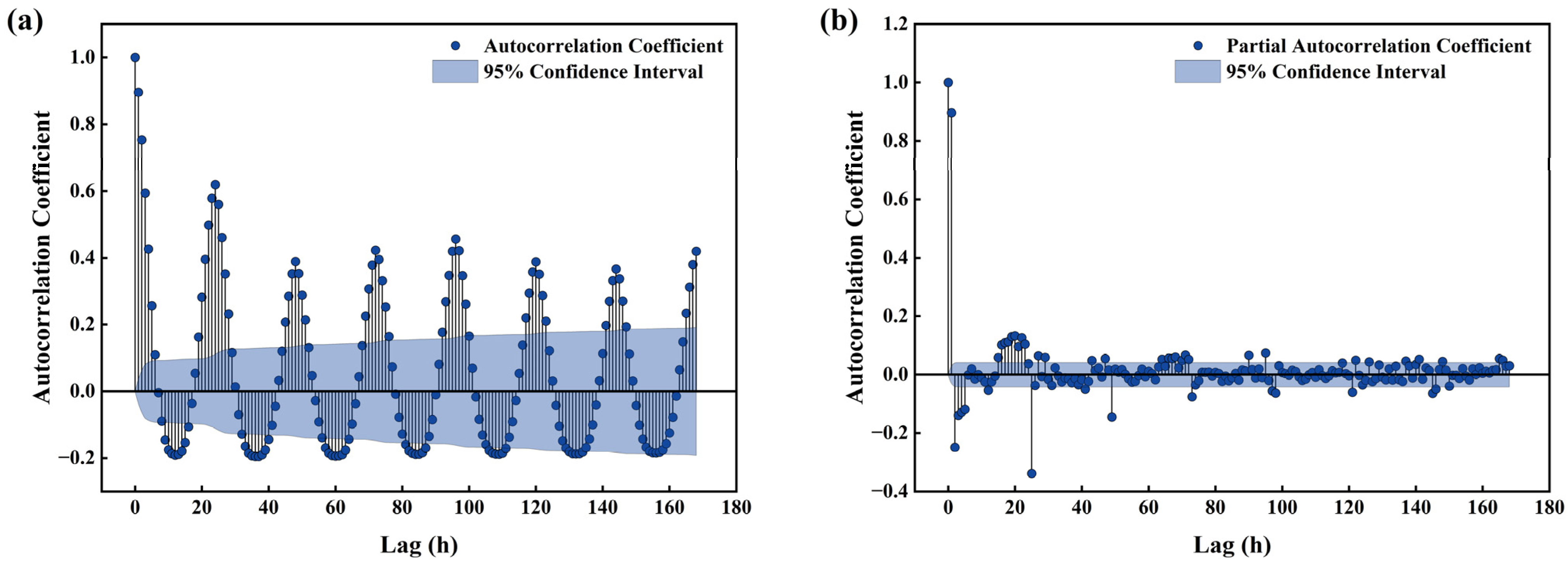
The time series prediction model used in this study is the CNN-LSTM-Attention (CLA) model, as shown in Figure A2 in Appendix C. The CLA model has demonstrated success across various domains. In time series forecasting, it offers distinct advantages by effectively capturing both short-term fluctuations and long-term trends in the data [47,48]. In this study, the CNN component extracts key features from meteorological data, such as temperature, precipitation, and wind speed, to identify relevant patterns. The LSTM component captures temporal dependencies, learning from historical climate trends to predict how long-term changes, like rising temperatures, influence migration timing and intensity. The attention mechanism then highlights important interactions between meteorological factors, dynamically adjusting their impact to better represent the complex relationships between climate variables and bird migration. This integrated approach allows the model to accurately capture the dynamics of climate impacts on migration.

The 48 h moving window used in the model is both scientifically grounded and pragmatically efficient. It captures both short-term and long-term dependencies, ensuring that the model can accurately forecast bird activity patterns while maintaining sensitivity to cyclical changes. This approach provides a solid framework for prediction, leveraging key temporal structures in the data while preserving the model’s overall predictive accuracy. Mao employed a GRU-based model with attention mechanisms to predict bird migration [49]. While this method captured temporal dependencies, it struggled with feature extraction, limiting its performance. Our study combined CNN and LSTM, improving feature extraction and handling long-term dependencies more effectively, leading to more accurate predictions. Additionally, Mao removed missing values, which could lead to data loss [49]. In contrast, our study used predictive interpolation to estimate missing values, preserving data integrity and enhancing the reliability of the results.

3.5.1. MTR Prediction

During the regression interpolation of missing data, particularly near zero, the model may struggle to accurately estimate low-intensity values, which can result in fluctuations and negative MTR predictions. In temporal predictions, the model faces difficulties when attempting to fit all data points, especially when the data include extreme values or high volatility. This can lead to negative predictions if the model does not adequately adapt to local patterns or abrupt changes. These issues are particularly noticeable when the data are sparse. To address these challenges, we replaced negative values in the interpolated data with the nearest non-negative value from a time point that is 24 h apart. This ensures the predictions are consistent with expected migration patterns and prevents unrealistic negative values. Additionally, we incorporated the rectified linear units (ReLU) activation function [50] in the final stage of the nonlinear regression model. Instead of using ReLU as a post-prediction correction, we applied it during training. When the model predicts negative values, the ReLU activation increases the loss, prompting the model to adjust its predictions. This active correction, embedded in the training process, helps the model avoid negative predictions, especially when positive values are expected. Thus, ReLU is an essential part of the learning process, guiding the model to minimize negative predictions and ensuring accurate, non-negative migration values without the need for post-prediction adjustments. These two solutions ensure that the model generates accurate, non-negative predictions that align with real-world migration patterns while maintaining its adaptability and minimizing prediction errors.

Figure 6 and Figure 7 show the prediction performance of the CLA model on bird migration intensity (MTR) across five cities during the spring and autumn migration seasons. The model effectively captures the main trends and fluctuations in migration intensity, particularly during peak periods, where the predicted values closely match the actual data, demonstrating its accuracy in identifying peak migration changes. However, at lower intensity levels, especially when the intensity approaches zero, the model’s prediction accuracy decreases. The higher errors observed in the model during low migration periods are mainly due to the ecological differences between resident and migratory birds. Resident birds, which stay in fixed areas year-round, are driven by food availability, territorial behavior, and social interactions, showing little response to short-term weather changes. In contrast, migratory birds depend heavily on weather conditions, adjusting their activity levels based on factors such as wind, radiation, and stable air pressure. During low migration periods, the contribution of resident birds to the MTR increases, leading to a higher amount of background noise. This results in larger errors during interpolation and time-series prediction, affecting model accuracy. However, the impact of this error on the overall predictions remains minimal for migration safety applications. As algorithms for extracting bird activity-related data from weather radar continue to improve [51,52], data quality will progressively enhance over time. From an aviation safety perspective, the primary objective of the model is to predict high-risk migration periods when bird strikes are more likely. Errors during low-activity periods have minimal impact on the model’s overall utility for aviation safety, as these periods present a lower risk for bird strikes. Future work will focus on enhancing the model’s performance during low-activity periods by incorporating additional factors, such as habitat changes and human behavior. This will help better account for the behavior of resident birds and mitigate the effects of interpolation errors [42].

To address the small dataset issue, we incorporated additional data from the 2024 spring migration season to enhance the model’s generalization. We applied a “pre-training and fine-tuning” strategy [53], where the CLA model, initially trained on the 2023 data, was fine-tuned using the 2024 dataset. This process involved freezing the CNN layers and adjusting the parameters of the LSTM and attention layers. The results for the 2024 dataset, with an average R² of 0.8954 (compared to the original model’s R² of 0.9274), demonstrate the model’s robustness despite the meteorological variations across the years. These results are presented in Figure 8. This strategy is particularly beneficial in regions with sparse radar data, as it enables the model to adapt to new regions or conditions with minimal additional data, reducing the need for full retraining and computational costs. Additionally, the validation strategy, which includes cities with diverse climatic and ecological conditions, ensures the model’s effectiveness and generalizability across a wide range of meteorological scenarios.

To further compare the performance differences between the CLA model and more advanced models, we selected the Transformer model for evaluation due to its ability to capture complex, nonlinear relationships within the data, facilitated by its attention mechanism. This mechanism allows the model to focus on the most relevant features at different stages of migration, thereby improving its predictive accuracy, especially during periods of high migration intensity. The experimental results, presented in Figure 6 and Figure A3, show that although the Transformer model exhibits a slightly higher Mean Absolute Error (MAE) compared to the CLA model, it excels in capturing the intricate patterns of migration intensity, particularly during peak migration periods. Specifically, the CLA model achieved an average R² value of approximately 0.92, while the Transformer model achieved an average R² value of approximately 0.87. The comparison between Figure 6 and Figure A3 demonstrates how the Transformer model more effectively captures high-intensity migration events, which are critical for bird strike prevention in aviation. However, the results also highlight areas for improvement, particularly the need to reduce MAE during periods of low migration activity, which is essential for improving the model’s overall performance. In conclusion, the attention mechanism integrated into the Transformer model enables more nuanced and accurate predictions of migration intensity, particularly during high-risk periods. While challenges persist during low-activity phases, the Transformer model shows significant promise for real-time bird strike prediction systems. Future research will focus on refining Transformer variants based on the CLA model, incorporating additional features and optimization techniques to enhance its performance across all migration phases, ultimately improving both its robustness and predictive accuracy.

Overall, the model successfully meets the objective of predicting bird migration activity based on meteorological factors and achieves the expected outcomes. In comparison, a study by Xu et al., which used similar data to this research, employed the random forest model to predict migration activity. Their model achieved a prediction accuracy of around 75%, which increased to 82% after improving data quality [54]. In contrast, the model developed in our study consistently maintained a prediction accuracy of over 90% for MTR across different cities. This highlights the superior performance and robustness of our model compared to previous approaches. Our model predicts migration intensity based on current weather conditions, enabling airports to anticipate peak migration periods. This allows for early warning alerts to notify airport authorities of high-risk times, enabling timely adjustments to flight schedules or the implementation of additional safety measures. Additionally, the model can assist wildlife management by directing efforts to high-risk areas and can be integrated with existing bird detection systems, such as radar and tracking technologies. This integration provides a comprehensive view of bird activity, enabling more informed decision-making, such as adjusting flight paths or deploying deterrents, ultimately enhancing bird strike prevention. In summary, our model offers airports a proactive tool to anticipate bird strike risks, improve real-time decision-making, and ensure safer airport operations.

3.5.2. Ablation Experiments

To assess the contribution and necessity of each component within the overall model and further optimize its accuracy and robustness, a series of ablation experiments were conducted using spring migration data. By systematically removing or substituting certain structures within the model, the impact on model performance was evaluated, clarifying the role and importance of each module. Model performance was comprehensively evaluated using metrics such as Mean Squared Error (MSE), Root Mean Squared Error (RMSE), Mean Absolute Error (MAE), and the coefficient of determination (R²). The experimental results are summarized in

Table 2. Ablation experiment results.

City	Model	R2	MSE	RMSE	MAE
Zhangjiakou	I	0.9012	0.0023	0.0485	0.0337
	II	0.8348	0.0054	0.0737	0.0497
	III	0.8473	0.0034	0.0588	0.0370
	IV	0.7866	0.0048	0.0695	0.0529
Shijiazhuang	I	0.9191	0.0054	0.0735	0.0462
	II	0.8574	0.0027	0.0528	0.0318
	III	0.8192	0.0119	0.1093	0.0654
	IV	0.8099	0.0126	0.1126	0.0652
Zhengzhou	I	0.9485	0.0023	0.0484	0.0336
	II	0.9176	0.0057	0.0755	0.0481
	III	0.8742	0.0040	0.0639	0.0442
	IV	0.8511	0.0067	0.0818	0.0051
Yichang	I	0.9475	0.0015	0.0393	0.0249
	II	0.9133	0.0028	0.0536	0.0304
	III	0.8384	0.0047	0.0686	0.0456
	IV	0.8204	0.0052	0.0721	0.0437
Changsha	I	0.9210	0.0010	0.0330	0.0227
	II	0.9175	0.0033	0.0575	0.0386
	III	0.8345	0.0022	0.0469	0.0343
	IV	0.8215	0.0023	0.0484	0.0349

Notes: I: Baseline model, II: CNN-LSTM model, III: LSTM-Attention model, IV: LSTM model.

.

The results indicate that, compared to the benchmark model, the ability to handle long-distance dependencies is significantly reduced when the attention mechanism is removed. Removing the attention mechanism alone reduced the average prediction accuracy (R²) by 3.93%, while excluding both the CNN and attention mechanisms caused a more severe decline of 10.96%. The attention mechanism enhances the model’s capacity to process long sequence data by dynamically adjusting the focus on critical temporal intervals, such as nocturnal migration peaks. Although the CNN-LSTM model can effectively extract features and capture time series information, it performs worse than the benchmark model in handling long-distance dependencies. When the CNN component is removed, the model’s spatial feature extraction capability is notably diminished, reducing average R² by 8.47%. While the LSTM with the attention mechanism can adaptively weight sequential data, the absence of CNN preprocessing degraded initial feature representations, especially under rapidly changing meteorological conditions (e.g., sudden rainfall events). Removing both the CNN and attention mechanisms leaves the LSTM model to rely solely on itself for processing the raw data. This simplification reduced accuracy by 10.96%. Although LSTM can capture temporal dependencies, its performance deteriorates significantly without the benefit of feature extraction and dynamic attention adjustment, leading to an overall performance lower than that of the benchmark model. The ablation experiments highlight the contributions of each component: CNNs effectively extract high-level features, LSTM captures time series dependencies, and the attention mechanism enhances the ability to handle long-distance dependencies. By fully integrating the strengths of these modules, the benchmark model outperforms models that lack any single component. These findings provide valuable insights for optimizing future model designs.

Our study demonstrates the effectiveness of the CLA model in predicting bird migration intensity. However, several avenues for future research could further enhance its performance and applicability. One promising direction is the integration of advanced Transformer variants, such as Informer [55] and Autoformer [56]. These models have shown considerable success in forecasting long-sequence time series [57,58,59]. I Informer improves computational efficiency through its sparse attention mechanism and excels in long-term sequence prediction tasks. Compared to traditional Transformers, Informer is better suited to handle large-scale time series data. In contrast, Autoformer uses a seasonal decomposition strategy to manage different components of time series, enhancing its ability to model seasonality and trends. Another potential direction is the use of state space models, such as Mamba [60]. This model achieves linear time complexity in sequence modeling, offering high accuracy and low computational cost for long-sequence tasks. Although still in the early stages, Mamba shows great potential for real-time bird activity monitoring, especially in scenarios requiring rapid responses.

4. Conclusions

This study examined how meteorological and temporal factors influence bird migration intensity, using weather radar and meteorological data from five cities along China’s central migration route. A CLA model, which integrates CNN, LSTM, and an attention mechanism, was developed to capture the complex spatiotemporal dynamics of migration. The model achieved over 90% accuracy across different cities and seasons. The use of a 48 h sliding window improved both stability and prediction precision, demonstrating the model’s effectiveness in handling long-term dependencies and local feature extraction. The findings show that both meteorological conditions and temporal characteristics are key to migration intensity and patterns. Diffuse horizontal irradiance had the most significant impact on migration intensity. Lower radiation levels during nocturnal migration help birds conserve energy. Additionally, wind conditions and air pressure also influence migration intensity, though to a lesser extent. Temporal factors, such as migration timing, affect the cycle, with peak intensity observed in late April to early May in spring and mid-September to early October in autumn.

While the study provides valuable insights, it is limited by a small dataset due to data acquisition challenges. Future research should focus on improving the model’s performance with sparse and noisy data, especially in areas with limited radar coverage. Techniques like data augmentation, transfer learning, and domain adaptation could further enhance the model’s robustness. Moreover, incorporating factors such as land use, vegetation, and human activity would improve prediction accuracy and contribute to more effective conservation strategies.

References

1. Metz, I.C.; Ellerbroek, J.; Mühlhausen, T.; Kügler, D.; Hoekstra, J.M. The Bird Strike Challenge. Aerospace 2020, 7, 26. [Google Scholar] [CrossRef]
2. Carey, C. The Impacts of Climate Change on the Annual Cycles of Birds. Philos. Trans. R. Soc. B Biol. Sci. 2009, 364, 3321–3330. [Google Scholar] [CrossRef] [PubMed]
3. Dokter, A.M.; Farnsworth, A.; Fink, D.; Ruiz-Gutierrez, V.; Hochachka, W.M.; La Sorte, F.A.; Robinson, O.J.; Rosenberg, K.V.; Kelling, S. Seasonal Abundance and Survival of North America’s Migratory Avifauna Determined by Weather Radar. Nat. Ecol. Evol. 2018, 2, 1603–1609. [Google Scholar] [CrossRef] [PubMed]
4. Nussbaumer, R.; Bauer, S.; Benoit, L.; Mariethoz, G.; Liechti, F.; Schmid, B. Quantifying Year-Round Nocturnal Bird Migration with a Fluid Dynamics Model. J. R. Soc. Interface 2021, 18, 20210194. [Google Scholar] [CrossRef]
5. DeVault, T.L.; Blackwell, B.F.; Seamans, T.W.; Begier, M.J.; Kougher, J.D.; Washburn, J.E.; Miller, P.R.; Dolbeer, R.A. Estimating Interspecific Economic Risk of Bird Strikes with Aircraft. Wildl. Soc. Bull. 2018, 42, 94–101. [Google Scholar] [CrossRef]
6. Alerstam, T. Wind as Selective Agent in Bird Migration. Ornis Scand. Scand. J. Ornithol. 1979, 10, 76–93. [Google Scholar] [CrossRef]
7. Koleček, J.; Adamík, P.; Reif, J. Shifts in Migration Phenology under Climate Change: Temperature vs. Abundance Effects in Birds. Clim. Chang. 2020, 159, 177–194. [Google Scholar] [CrossRef]
8. Studds, C.E.; Marra, P.P. Rainfall-Induced Changes in Food Availability Modify the Spring Departure Programme of a Migratory Bird. Proc. R. Soc. B Biol. Sci. 2011, 278, 3437–3443. [Google Scholar] [CrossRef]
9. Gerson, A.R.; Guglielmo, C.G. Flight at Low Ambient Humidity Increases Protein Catabolism in Migratory Birds. Science 2011, 333, 1434–1436. [Google Scholar] [CrossRef]
10. Komal, R.; Khushboo; Dwivedi, A.; Vaish, V.; Rani, S. Conquering the Night: Understanding Nocturnal Migration in Birds. Biol. Rhythm Res. 2017, 48, 747–755. [Google Scholar] [CrossRef]
11. Horton, K.G.; La Sorte, F.A.; Sheldon, D.; Lin, T.-Y.; Winner, K.; Bernstein, G.; Maji, S.; Hochachka, W.M.; Farnsworth, A. Phenology of Nocturnal Avian Migration Has Shifted at the Continental Scale. Nat. Clim. Chang. 2020, 10, 63–68. [Google Scholar] [CrossRef]
12. Cohen, E.B.; Buler, J.J.; Horton, K.G.; Loss, S.R.; Cabrera-Cruz, S.A.; Smolinsky, J.A.; Marra, P.P. Using Weather Radar to Help Minimize Wind Energy Impacts on Nocturnally Migrating Birds. Conserv. Lett. 2022, 15, e12887. [Google Scholar] [CrossRef]
13. Elmore, J.A.; Riding, C.S.; Horton, K.G.; O’Connell, T.J.; Farnsworth, A.; Loss, S.R. Predicting Bird-Window Collisions with Weather Radar. J. Appl. Ecol. 2021, 58, 1593–1601. [Google Scholar] [CrossRef]
14. Pancerasa, M.; Sangiorgio, M.; Ambrosini, R.; Saino, N.; Winkler, D.W.; Casagrandi, R. Reconstruction of Long-Distance Bird Migration Routes Using Advanced Machine Learning Techniques on Geolocator Data. J. R. Soc. Interface 2019, 16, 20190031. [Google Scholar] [CrossRef]
15. Akçay, H.G.; Kabasakal, B.; Aksu, D.; Demir, N.; Öz, M.; Erdoğan, A. Automated Bird Counting with Deep Learning for Regional Bird Distribution Map. Animals 2020, 10, 1207. [Google Scholar] [CrossRef]
16. Lostanlen, V.; Cramer, A.; Salamon, J.; Farnsworth, A.; Doren, B.M.V.; Kelling, S.; Bello, J.P. BirdVox: Machine Listening for Bird Migration Monitoring. bioRxiv 2022. [Google Scholar] [CrossRef]
17. Strobl, C.; Malley, J.; Tutz, G. An Introduction to Recursive Partitioning: Rationale, Application, and Characteristics of Classification and Regression Trees, Bagging, and Random Forests. Psychol. Methods 2009, 14, 323–348. [Google Scholar] [CrossRef]
18. Santhanam, R.; Uzir, N.; Raman, S.; Banerjee, S. Experimenting XGBoost Algorithm for Prediction and Classification of Different Datasets. Int. J. Control. Theory Appl. 2016, 9, 651–662. [Google Scholar]
19. Liang, W.; Luo, S.; Zhao, G.; Wu, H. Predicting Hard Rock Pillar Stability Using GBDT, XGBoost, and LightGBM Algorithms. Mathematics 2020, 8, 765. [Google Scholar] [CrossRef]
20. Hancock, J.T.; Khoshgoftaar, T.M. CatBoost for Big Data: An Interdisciplinary Review. J. Big Data 2020, 7, 64. [Google Scholar] [CrossRef]
21. Dhaliwal, S.S.; Nahid, A.-A.; Abbas, R. Effective Intrusion Detection System Using XGBoost. Information 2018, 9, 149. [Google Scholar] [CrossRef]
22. Ke, G.; Meng, Q.; Finley, T.; Wang, T.; Chen, W.; Ma, W.; Ye, Q.; Liu, T.-Y. LightGBM: A Highly Efficient Gradient Boosting Decision Tree. In Proceedings of the Advances in Neural Information Processing Systems; Curran Associates, Inc.: Red Hook, NY, USA, 2017; Volume 30. [Google Scholar]
23. Huang, G.; Wu, L.; Ma, X.; Zhang, W.; Fan, J.; Yu, X.; Zeng, W.; Zhou, H. Evaluation of CatBoost Method for Prediction of Reference Evapotranspiration in Humid Regions. J. Hydrol. 2019, 574, 1029–1041. [Google Scholar] [CrossRef]
24. Mohamed, K.S. Brain-Inspired Machine Learning Algorithm: Neural Network Optimization. In Machine Learning for Model Order Reduction; Springer: Cham, Switzerland, 2018; pp. 65–74. ISBN 978-3-319-75714-8. [Google Scholar]
25. Sherstinsky, A. Fundamentals of Recurrent Neural Network (RNN) and Long Short-Term Memory (LSTM) Network. Phys. Nonlinear Phenom. 2020, 404, 132306. [Google Scholar] [CrossRef]
26. Li, Z.; Liu, F.; Yang, W.; Peng, S.; Zhou, J. A Survey of Convolutional Neural Networks: Analysis, Applications, and Prospects. IEEE Trans. Neural Netw. Learn. Syst. 2022, 33, 6999–7019. [Google Scholar] [CrossRef]
27. Liu, J.W.; Liu, J.W.; Luo, X.L. Research progress in attention mechanism in deep learning. Chin. J. Eng. 2021, 43, 1499–1511. [Google Scholar] [CrossRef]
28. Dokter, A.M.; Desmet, P.; Spaaks, J.H.; van Hoey, S.; Veen, L.; Verlinden, L.; Nilsson, C.; Haase, G.; Leijnse, H.; Farnsworth, A.; et al. bioRad: Biological Analysis and Visualization of Weather Radar Data. Ecography 2019, 42, 852–860. [Google Scholar] [CrossRef]
29. Chen, K.; Kross, S.M.; Parkins, K.; Seewagen, C.; Farnsworth, A.; Van Doren, B.M. Heavy Migration Traffic and Bad Weather Are a Dangerous Combination: Bird Collisions in New York City. J. Appl. Ecol. 2024, 61, 784–796. [Google Scholar] [CrossRef]
30. Xi, J.; Deng, X.; Zhao, G.; Batbayar, N.; Damba, I.; Zhao, Q.; Cui, S.; Jiang, C.; Chen, Y.; Yu, Y.; et al. Migration Routes, Behavior and Protection Status of Eurasian Spoonbills (Platalea leucorodia) Wintering in China. Avian Res. 2021, 12, 70. [Google Scholar] [CrossRef]
31. Kuang, F.; Coleman, J.T.; Hassell, C.J.; Leung, K.-S.K.; Maglio, G.; Ke, W.; Cheng, C.; Zhao, J.; Zhang, Z.; Ma, Z. Seasonal and Population Differences in Migration of Whimbrels in the East Asian–Australasian Flyway. Avian Res. 2020, 11, 24. [Google Scholar] [CrossRef]
32. Dahouda, M.K.; Joe, I. A Deep-Learned Embedding Technique for Categorical Features Encoding. IEEE Access 2021, 9, 114381–114391. [Google Scholar] [CrossRef]
33. Azodi, C.B.; Tang, J.; Shiu, S.-H. Opening the Black Box: Interpretable Machine Learning for Geneticists. Trends Genet. 2020, 36, 442–455. [Google Scholar] [CrossRef] [PubMed]
34. Mangalathu, S.; Hwang, S.-H.; Jeon, J.-S. Failure Mode and Effects Analysis of RC Members Based on Machine-Learning-Based SHapley Additive exPlanations (SHAP) Approach. Eng. Struct. 2020, 219, 110927. [Google Scholar] [CrossRef]
35. Helm, B.; Liedvogel, M. Avian Migration Clocks in a Changing World. J. Comp. Physiol. A 2024, 210, 691–716. [Google Scholar] [CrossRef]
36. Liu, S.; Townshend, T.; Farnsworth, A.; Alexander, D.; Tian, H.; Hua, F. Monitoring Bird Migration Using Nocturnal Flight Calls on the East Asian–Australasian Flyway: A Case from Beijing. Bird Conserv. Int. 2024, 34, e19. [Google Scholar] [CrossRef]
37. Marcílio, W.E.; Eler, D.M. From Explanations to Feature Selection: Assessing SHAP Values as Feature Selection Mechanism. In Proceedings of the 2020 33rd SIBGRAPI Conference on Graphics, Patterns and Images (SIBGRAPI), Virtual, 7–10 November 2020; pp. 340–347. [Google Scholar]
38. Cooper, N.W.; Dossman, B.C.; Berrigan, L.E.; Brown, J.M.; Cormier, D.A.; Bégin-Marchand, C.; Rodewald, A.D.; Taylor, P.D.; Tremblay, J.A.; Marra, P.P. Atmospheric Pressure Predicts Probability of Departure for Migratory Songbirds. Mov. Ecol. 2023, 11, 23. [Google Scholar] [CrossRef]
39. Byrd, A.J.; Talbott, K.M.; Smiley, T.M.; Verrett, T.B.; Gross, M.S.; Hladik, M.L.; Ketterson, E.D.; Becker, D.J. Determinants of Spring Migration Departure Dates in a New World Sparrow: Weather Variables Reign Supreme. Ecol. Evol. 2024, 14, e10874. [Google Scholar] [CrossRef]
40. Xu, Q.; Liu, J.; Su, M.; Chen, W. Quantitative Bird Activity Characterization and Prediction Using Multivariable Weather Parameters and Avian Radar Datasets. Aerospace 2023, 10, 462. [Google Scholar] [CrossRef]
41. Benjumea, R.; Astrain, C.; Istúriz, A.; Oria, P.; Ibarrola, I.; del Mar Delgado, M. Weather Conditions at Different Spatial and Temporal Scales Influence Avian Post-Breeding Migration Patterns on Route. J. Zool. 2024, 323, 305–316. [Google Scholar] [CrossRef]
42. van Gasteren, H.; Krijgsveld, K.L.; Klauke, N.; Leshem, Y.; Metz, I.C.; Skakuj, M.; Sorbi, S.; Schekler, I.; Shamoun-Baranes, J. Aeroecology Meets Aviation Safety: Early Warning Systems in Europe and the Middle East Prevent Collisions between Birds and Aircraft. Ecography 2019, 42, 899–911. [Google Scholar] [CrossRef]
43. Kranstauber, B.; Bouten, W.; van Gasteren, H.; Shamoun-Baranes, J. Ensemble Predictions Are Essential for Accurate Bird Migration Forecasts for Conservation and Flight Safety. Ecol. Solut. Evid. 2022, 3, e12158. [Google Scholar] [CrossRef]
44. Scott, K.M.; Danko, A.; Plant, P.; Dakin, R. What Causes Bird-Building Collision Risk? Seasonal Dynamics and Weather Drivers. Ecol. Evol. 2023, 13, e9974. [Google Scholar] [CrossRef] [PubMed]
45. Hansen, P.R.; Lunde, A. Estimating the persistence and the autocorrelation function of a time series that is measured with error. Econom. Theory 2014, 30, 60–93. [Google Scholar] [CrossRef]
46. Ramsey, F.L. Characterization of the Partial Autocorrelation Function. Ann. Stat. 1974, 2, 1296–1301. [Google Scholar] [CrossRef]
47. Wan, A.; Chang, Q.; AL-Bukhaiti, K.; He, J. Short-Term Power Load Forecasting for Combined Heat and Power Using CNN-LSTM Enhanced by Attention Mechanism. Energy 2023, 282, 128274. [Google Scholar] [CrossRef]
48. Yang, Y.; Xiong, Q.; Wu, C.; Zou, Q.; Yu, Y.; Yi, H.; Gao, M. A Study on Water Quality Prediction by a Hybrid CNN-LSTM Model with Attention Mechanism. Environ. Sci. Pollut. Res. 2021, 28, 55129–55139. [Google Scholar] [CrossRef]
49. Mao, H.; Hu, C.; Wang, R.; Cui, K.; Wang, S.; Kou, X.; Wu, D. Deep-Learning-Based Flying Animals Migration Prediction With Weather Radar Network. IEEE Trans. Geosci. Remote Sens. 2023, 61, 1–13. [Google Scholar] [CrossRef]
50. Agarap, A.F. Deep Learning Using Rectified Linear Units (ReLU). arXiv 2019. [Google Scholar] [CrossRef]
51. Shi, X.; Drucker, J.; Chapman, J.W.; Herrera, M.S.; Dokter, A.M. Analysis of Mixtures of Birds and Insects in Weather Radar Data. bioRxiv 2024. [Google Scholar] [CrossRef]
52. Weisshaupt, N.; Harnist, B.; Koistinen, J. The Impact of Dealiasing Biases on Bird and Insect Data Products of C-Band Weather Radars and Consequences for Aeroecological Applications. Remote Sens. 2025, 17, 436. [Google Scholar] [CrossRef]
53. Gao, T.; Fisch, A.; Chen, D. Making Pre-Trained Language Models Better Few-Shot Learners. arXiv 2021. [Google Scholar] [CrossRef]
54. Xu, Q.; Liu, J.; Su, M.; Chen, W.S. Bird Behaviour Characterisation and Environment Dependence Modelling in Airport Airspace Based on Radar Datasets. Aeronaut. J. 2024, 128, 2815–2831. [Google Scholar] [CrossRef]
55. Zhou, H.; Zhang, S.; Peng, J.; Zhang, S.; Li, J.; Xiong, H.; Zhang, W. Informer: Beyond Efficient Transformer for Long Sequence Time-Series Forecasting. arXiv 2021. [Google Scholar] [CrossRef]
56. Wu, H.; Xu, J.; Wang, J.; Long, M. Autoformer: Decomposition Transformers with Auto-Correlation for Long-Term Series Forecasting. arXiv 2022. [Google Scholar] [CrossRef]
57. Tian, X.; Zhang, C.; Liu, H.; Zhang, B.; Lu, C.; Jiao, P.; Ren, S. Research on Air Quality in Response to Meteorological Factors Based on the Informer Model. Sustainability 2024, 16, 6794. [Google Scholar] [CrossRef]
58. Xu, Y.; Zhao, J.; Wan, B.; Cai, J.; Wan, J. Flood Forecasting Method and Application Based on Informer Model. Water 2024, 16, 765. [Google Scholar] [CrossRef]
59. Feng, H.; Zhang, X. A Novel Encoder-Decoder Model Based on Autoformer for Air Quality Index Prediction. PLoS ONE 2023, 18, e0284293. [Google Scholar] [CrossRef]
60. Gu, A.; Dao, T. Mamba: Linear-Time Sequence Modeling with Selective State Spaces. arXiv 2024. [Google Scholar] [CrossRef]
Figure 1. Relative contribution of (a) monthly feature and (b) hourly feature during spring migration.
Sustainability 17 02793 g001
Figure 2. The scatter plots of SHAP values for meteorological factors in (a) Zhangjiakou, (b) Shijiazhuang, (c) Zhengzhou, (d) Yichang, and (e) Changsha during spring migration.
Sustainability 17 02793 g002
Figure 3. Relative contribution of (a) monthly feature and (b) hourly feature during autumn migration.
Sustainability 17 02793 g003
Figure 4. The scatter plots of SHAP values for meteorological factors in (a) Zhangjiakou, (b) Shijiazhuang, (c) Zhengzhou, and (d) Yichang during autumn migration.
Sustainability 17 02793 g004
Figure 5. Relative contribution of meteorological factors to migration intensity during (a) spring and (b) autumn migration.
Sustainability 17 02793 g005
Figure 6. Comparison of Predicted and Observed MTR Values in (a) Zhangjiakou, (b) Shijiazhuang, (c) Zhengzhou, (d) Yichang, and (e) Changsha during the 2023 spring migration.
Sustainability 17 02793 g006
Figure 7. Comparison of Predicted and Observed MTR Values in (a) Zhangjiakou, (b) Shijiazhuang, (c) Zhengzhou, and (d) Yichang during the 2023 autumn migration.
Sustainability 17 02793 g007
Figure 8. Comparison of Predicted and Observed MTR Values in (a) Zhangjiakou, (b) Shijiazhuang, (c) Zhengzhou, (d) Yichang and (e) Changsha during the 2024 spring migration.
Sustainability 17 02793 g008