Analysis of the Interaction Between Endogenous Technological Innovation, Institutional Regulation, and Economic Long Wave: A Perspective from Nonlinear Dynamics

Abstract

The capitalist economy has experienced several economic long waves after the industrial revolution. The previous explanations for their causes have primarily focused on a single factor such as technology or institution, which has limitations and flaws. In this paper, the cause of economic long waves is explained by employing the nonlinear interaction and nonequilibrium evolution mechanisms in complex economics. Moreover, the relationships between endogenous technological innovation, institutional regulation, and economic long waves are examined. The research results show that technological innovation is driven by the economic long wave movement. In particular, the phases of depression, recovery, and prosperity within these waves may serve as catalysts for further innovation. The free market can exhibit endogenous instability. The dual regulation of productive and distributive institutions can ensure stable and efficient economic development and achieve broad social benefits. However, in a context of individual decentralized decision making, the institutional structures often deviate from the optimal outcome. This deviation, to a certain extent, leads to structural economic crises. The integration and interaction between technological innovation and institutional regulation jointly drive the long wave movement and the accumulation cycle of the economy. This paper proposes a feasible method for studying economic long waves, offering insights that could promote sustainable and robust economic development.

1. Introduction

Capitalism has experienced several long-term cyclical phenomena of relatively stable economic growth and alternating crises since the industrial revolution. This economic cyclical fluctuation lasting about 45–60 years is called the Kondratiev long wave [1,2,3]. As we all know, the economic long wave consists of two phases: an upward period and a decline period, therefore an appropriate long wave theory must explain how each phase is formed. It is a challenging and controversial task to explain the causes of long waves, and there are different views in academia, including technology long wave theory [4,5,6,7,8,9,10], the institution long wave theory [11,12,13,14], and the endogenous long wave theory [15,16,17].

The technology long wave theory identifies technological innovation as the leading factor in economic long wave movements. Schumpeter, the founder of this theory, argued that innovation was the core driving force of economic long wave movement, believing that the emergence of innovation propels the economy into a prosperous (upward) stage; conversely, when the potential for innovation is exhausted, the economy enters the recession (decline) phase [4]. For example, from the late 18th to the early 19th century, the invention and application of the steam engine triggered a series of technological innovations, which promoted the rapid development of industries such as textiles and metallurgy and initiated the upward stage of the economic long wave. Mensch and Van Duijn of the neo-Schumpeter school argued that the limited possibility of further technological improvement or market saturation caused the economy to transition from a prosperous stage to a stagnant stage. Mensch [18] believed that the stagnation of existing technology marked the decline period of long waves, linking technological innovation with economic depression and asserting the lack of breakthrough innovations was the main reason for depression. Van Duijn [19] further pointed out that the economy in the depression stage could not be recovered quickly due to the stagnation of technological innovation, but it could not explain the decline period of long waves. The reason for the long wave decline period was that the stagnation of technological innovation leads to the completion of infrastructure, resulting in a significant decrease in infrastructure investment.

Regarding the causes of the upward period of long waves, the technology long wave theory regards technological innovation as the driving force of the economy; however, there is no consensus on what motivates enterprise technological innovation. Based on the different research perspectives, two theories have emerged: depression-induced and demand-pull theories. Mensch [18], a representative of the depression-induced theory, proposed that, during the depression stage of the economic long wave, the stagnation of old technologies and industries would stimulate the emergence of new clusters of basic innovations, thereby leading the economy out of the depression and into a new upward period. For example, after the great depression in the 1930s, innovations in emerging industries such as electronics and aviation drove economic recovery and a new round of growth. Regarding the viewpoint that depression forces enterprises to innovate, the argument is that investors are motivated to bear the high risks associated with basic innovation when the old technologies are no longer viable and profits are too low to sustain enterprises during the depression period. Consequently, clusters of innovations emerge at this stage. In contrast, Schmookler’s hypothesis [20], the representative of the demand-pull theory, asserted that a favorable economic environment is a necessary condition for innovation, and the innovation would be driven by an increase in demand; under this view, depression would actually inhibit innovation. Van Duijn [19] synthesized these two theories by classifying innovation into new industry product innovation, existing industry product innovation, existing industry process innovation, and the basic sector process innovation. Among these, the existing industry product innovation typically appears during depression and recovery stages, while the others tend to appear during depression, recovery, and prosperity stages, respectively.

As the representative of the theory of institutional long waves, the social structure accumulation (SSA) school within the western Marxist tradition links the economic long waves in capitalist history to the cycles of structure change in capitalist institutions, attempting to explain the long-term expansion, stagnation, and contraction of capitalist economies. The causes of the long wave upward period are attributed to the fact that the system provides stable and favorable conditions for capitalism by SSA, including profitable investment opportunities and a stable social environment; conversely, the decline period is attributed to the exhaustion of the investment profit opportunities inherent in the existing SSA [21]. However, Martin Wolfson and David Kotz, in their published articles, argued that the historical relationship between SSA theory and long wave theory should be re-evaluated to improve the persuasiveness and logicality of SSA theory [22]. They found that the proposed pattern of neoliberal SSA did not restore the economic growth rate and capital accumulation rate in the United States (U.S.), a theoretical dilemma stemming from SSA theory’s neglect of technical factors. In fact, the long-term decline in the U.S. economic growth rate and capital accumulation rate can be fully explained by the decrease in average profit margin caused by the improvement of the organic composition of capital.

In the theory of interaction between technology and institution, Perez’s viewpoint [23], a key perspective of neo-Schumpeter school, is particularly influential. She explained the long wave movement from the rupture and re-coupling of the relationship between economy and institution during the diffusion process of technological revolution. The development tide of technological revolution diffusion underwent two distinct stages: the import period and the expansion period. During the import period, the power of technological revolution gradually increased and demonstrated enormous potential for wealth creation. However, the increasingly evident mismatch between the economy and the old institution created resistance to the further spread of technological revolution. The structural tension ended the initial outbreak and frenzy, leading to a serious recession and depression, after which a new institutional structure began to emerge. In the expansion period, the “creative destruction of the system” facilitated the re-coupling of the relationship between economy and institutions, ushering the golden age in which the technological revolution could fully unleash its potential. Perez’s analysis aligns closely with Marxist historical materialism.

Whether it is the institutional long wave theory or the technology and institutional interaction long wave theory, institutions, in a broad sense, include politics, economy, culture, and so on. SSA theory holds that institutions help to alleviate class contradictions and stabilize capitalist expectations. Perez pointed out that the institution played a role by releasing the potential of technological change. In fact, the institution itself has diversity, and the ways and effects of different institutions will inevitably show differences. A complete explanation of the causes and endogenous movements of economic long waves depends on a creative synthesis of Marxist economics and Schumpeter school economics. According to the perspective of Marxist economics, the economic cycle, including the economic long wave, results from the inherent contradiction within capital. Complexity science provides a powerful analytical framework. So-called complexity refers to nonlinear interaction and unbalanced evolution. Complex economics studies how the economy operates when it is in an unbalanced state [24,25]. Takuro Uehara et al. constructed a fully dynamic ecological–economic model to analyze the impacts of industrial ports on fish nursery habitats, which provides an important reference for eco-economic system research and policy formulation [26]. Jahanshahi et al. proposed a modeling approach for economic systems with variable-order fractional derivatives and designed a nonlinear model predictive controller, offering a new method for studying and controlling economic system dynamics [27]. Nonlinear dynamics, one of the main techniques used in complex economics, not only describes the endogenous fluctuations of economic systems using a limit cycle solution or chaotic solution but also depicts the qualitative change in economic structure caused by technological innovation and institutional adjustment based on the bifurcation theory. Bischi [28] illustrated the impact of multiplier-acceleration number models on economic dynamics, exploring the application of nonlinear dynamical systems in economic modeling, structural stability, and bifurcation theory. Ping Chen revealed lifecycles in the coevolution of ecology, technology, and culture based on the nonlinear dynamics of the division of labor and the theory of metabolic growth [29]. Semmler W et al. established corridor stability and local resilience to study the interaction of real and financial variables, where the trajectories may be stable or unstable near equilibrium, as explained by the Hopf and Bautin bifurcation theorems [30]. Parui Pintu investigated the influence of various parameters on the equilibrium values of debt–capital ratio and the growth rate using limit cycle solutions and the bifurcation theory [31].

In this paper, we focus on the views of neo-Schumpeter school and Marxist economists, analyzing the causes of economic long waves from the perspective of complex economics and constructing a dynamic theoretical model to discuss the realization of the law of values, while revealing the possibility of endogenous instability in the free market. In addition, we discuss the relationships between endogenous technological innovation, institutional regulation, and economic long waves after incorporating improvement innovation, breakthrough innovation, and basic innovation. The results indicate that technological innovation is caused by the economic long wave movement and that depression, recovery, and prosperity in the economic long wave may serve as the inducing factors for technological innovation. Moreover, under the conditions of individual decentralized decision making, institutional structures often deviate from the optimal configuration for stable and efficient economic development, leading to structural economic crises after deviating to a certain extent. The integration and interaction of technological innovation and institutional regulation jointly drive the long wave movement and the economic accumulation cycle. This paper provides a practical and feasible approach for the study of economic long waves.

The remainder of this study is structured as follows: the second section presents the model and theory of the structure and dynamics. Section 3 discusses the interaction between endogenous technological innovation, institutional regulation, and economic long waves along with the results. Section 4 presents empirical analyses on the rise of the information technology industry and the consolidation and decline of neoliberal SSA using the constructed model. Finally, Section 5 offers the conclusions of the study, presenting limitations and future study directions.

2. Model and Theory

Ping Chen employed the logistic equation from theoretical biology to describe the limited growth of products and technologies [32], which is different from the AK model in the neoclassical economic growth theory that is characterized by no resource constraints and constant returns to scale [33]. Ping Chen’s model lacks a limit cycle or chaotic solution, and it is unsuitable for simultaneously analyzing economic long waves and shorter-term economic fluctuations (such as medium waves). Therefore, we construct a more appropriate model with limited growth to investigate the law of economic cycle fluctuations. The detailed process of modeling the structure and dynamics is as follows.

Assuming that the production of innovative products is not limited by consumer demand or production technology, the effective production capacity $X$ changes at a constant growth rate $\gamma >0$:

$${\displaystyle \frac{dX}{dt}}=\gamma X$$

(1)

Equation (1) describes the evolution of the actual quantity of innovative products under the assumption of full capacity utilization, i.e., 100% capacity utilization. However, considering the real-world conditions, it is necessary to introduce the consumer demand constraints and the production technology constraints into the benchmark Equation (1) for innovative product growth to better reflect reality. Firstly, due to limited consumer demand, enterprises often operate below full capacity. We assume that the capacity utilization rate of innovative product $\mathrm{g}$ depends on the unmet effective demand or surplus market scale $Y$. When the consumer demand is saturated, enterprises lack the incentive to produce, and the capacity utilization rate drops to zero. Only when the remaining market size is positive will the capacity utilization rate exceed zero, and it increases with the surplus market scale. Therefore, the effective capacity utilization rate of innovative products is an increasing function to surplus market scale. However, it cannot increase indefinitely and will converge to a finite value as the surplus market scale tends towards positive infinity. A Michaelis–Menten equation can effectively describe the relationship between the capacity utilization rate of innovative product $g$ and the surplus market scale $Y$:

$$g(Y)={\displaystyle \frac{bY}{a+Y}}$$

(2)

where $b(0<b\le 1)$ represents the maximum capacity utilization rate for an innovative product, which is used to adjust the potential capacity utilization rate of the innovative product; and $a(a>0)$ is the semi-saturation constant for the surplus market scale, indicating that the effective capacity utilization rate reaches half of its maximum when the remaining market size equals $a$. Since only actual production leads to capital accumulation and effective capacity accumulation, the growth rate of effective capacity depends on actual output rather than effective capacity when actual output is below effective capacity. At this time, the number of innovative products is $g\left(Y\right)X$. Therefore, the effective capacity term in Equation (1) is replaced by actual output $g\left(Y\right)X$:

$${\displaystyle \frac{dX}{dt}}=\gamma g(Y)X$$

(3)

Thus, the growth rate of effective capacity reduced from $\gamma$ to $\gamma g\left(Y\right)$. The growth of effective production capacity and actual output is not only limited by effective demand but also by production technology since the production of goods requires a certain amount of living labor. If the value of innovative products and the remaining market size remain constant, any increase in product value implies a reduction in the degree of value realization, resulting in a relative decrease or even a negative value in surplus value realization. This hinders the capital accumulation and effective production capacity. To account for this, an exit term $-dX$ is added to the right of Equation (3):

$${\displaystyle \frac{dX}{dt}}=\gamma g(Y)X-dX$$

(4)

Here, $d(d>0)$ is the exit rate for innovative products. Thus, the effective capacity growth rate becomes $\gamma g\left(Y\right)-d$. Under certain conditions, variations in the parameter $d$ reflect changes in labor productivity: an increase in $d$ indicates a decline in labor productivity, reducing the surplus value realized by innovative products and consequently the capital accumulation rate, which in turn lowers the effective capacity growth rate.

In the traditional logistic equation, the surplus market size is analogous to nonrenewable resources and decreases as output increases. In contrast, the surplus market size can also expand, akin to renewable resources, and its net growth dynamic equation can be expressed as:

$${\displaystyle \frac{dY}{dt}}=rY\left(1-{\displaystyle \frac{Y}{N}}\right)-g(Y)X$$

(5)

where $N$ represents the saturation level of the surplus market size, and $r(r>0)$ is the proportional coefficient. The right-hand side of Equation (5) comprises two terms: the total growth rate and the exit rate. The second term implies that a portion of the consumption demand is met as a certain amount of innovative products are consumed, reducing the surplus market size by the same amount. The first term represents the total growth of the surplus market scale per unit time. Notably, when the surplus market is small, its total growth rate approximates $r$, but generally, the total growth rate of the surplus market scale exhibits an inverted U-shaped relationship with $Y$; beyond that value, the growth rate decreases as $Y$ increases. It is worth noting that there is a key positive feedback mechanism in the long wave model: as the surplus market scale expands (shrinks), its growth rate correspondingly increases (decreases). This endogenous instability mechanism in nonlinear dynamics arises from the organic combination of negative feedback and positive feedback, which is the comprehensive effect of forces tending towards equilibrium and forces moving away from equilibrium. This explains why adjusting production through the interaction between supply and demand does not necessarily tend to be balanced, which is a mathematical explanation of Marx’s theory of crisis possibility. It can be seen that the endogenous instability mechanism of nonlinear dynamics captures the contradictions and motion laws of things. Due to limited population size and consumption capacity, the surplus market also has an upper bound, represented by parameter $N$ in Equation (5). It is not difficult to understand that the social contagion mechanism and consumption incentive mechanism under a limited surplus market scale also lead to an inverted U relationship between the growth rate of the surplus market and its size. According to the theory of differential inequalities [34], it can be proven that the solution to the dynamical system composed of Equations (4) and (5) is bounded, resulting in limited demand and effective production capacity for innovative products, which directly leads to limited growth in the number of innovative products.

The technological innovation plays a fundamental role in the economic long wave movement, and it is itself endogenous, driven by capital accumulation associated with these long waves. In an industrial economy, technological innovation encompasses not only basic innovation but also improved and breakthrough technological innovation. The original model employed a fixed exit rate to describe the behavior of unimproved innovations and changes in unit commodity value. To incorporate factors of improved innovation into the basic innovation model, improved innovation is assumed to be a monotonically decreasing function of effective production capacity, thereby reducing the unit commodity value. Additionally, due to economies of scale, the unit commodity value decreases as effective production capacity expands. The improved innovation and economies of scale here can be considered to be jointly caused by the evolution of social division of labor (representing the interaction between enterprises) and the evolution of individual division of labor (representing the interaction between labor forces within enterprises). By modifying the exit term in Equations (4) and (5), we obtain

$${\displaystyle \frac{dX}{\mathrm{dt}}}=\gamma {\displaystyle \frac{b_{1}XY}{a_1+Y}}-\left(d+{\displaystyle \frac{b_2}{1+a_{2}X}}\right)X$$

(6)

$${\displaystyle \frac{dY}{\mathrm{dt}}}=rY\left(1-{\displaystyle \frac{Y}{N}}\right)-{\displaystyle \frac{b_{1}XY}{a_1+Y}}$$

(7)

where $X$ and $\gamma$ represent the effective production capacity and its constant growth rate under the assumption that the production of innovative products is not constrained by consumer demand or production technology.

The three types of technological innovation can be further clarified as follows. When $Y>0$, after the value of $X$ changes from zero to positive, the number of new products also becomes positive, which is basic innovation; as the effective production capacity $X$ increases, the exit term after the minus sign of Equation (6) decreases. The change in the exit term is related to the change in labor productivity, which is called improved technological innovation. The increase in parameter$a_2$ amplifies the role of increasing effective production capacity $X$, and the exit term decreases at a steeper speed, which is breakthrough technological innovation. There are eight parameters in the differential equation system. To facilitate analysis, we reduce the number of parameters by defining the variables and parameters as follows: $x=X$, $y=\gamma Y$, $\tau =rt$, ${\beta }_1={\displaystyle \frac{\gamma b_1}{r}}$, ${\beta }_2={\displaystyle \frac{b_2}{r}}$, $\delta ={\displaystyle \frac{d}{r}}$, ${\alpha }_1=\gamma a_1$, ${\alpha }_2=a_2$, and $K=\gamma N$. Consequently, the long wave dynamic equations are reformulated to contain six parameters and are obtained as follows:

$${\displaystyle \frac{dx}{d\tau }}={\displaystyle \frac{{\beta }_{1}xy}{{\alpha }_1+y}}-\delta x-{\displaystyle \frac{{\beta }_{2}x}{1+{\alpha }_{2}x}}$$

(8)

$${\displaystyle \frac{dy}{d\tau }}=y\left(1-{\displaystyle \frac{y}{K}}\right)-{\displaystyle \frac{{\beta }_{1}xy}{{\alpha }_1+y}}$$

(9)

3. Results and Discussion

If the direct results of parameter changes caused by technological progress, institutional regulation, or other factors are equivalent, then the effects of these factors can be modeled by adjusting the parameters. In Equation (9), both parameters ${\alpha }_1$ and $K$ are associated with the distributive institutional structure. Consider a situation where adjustments in the institutional structure lead to an increased share of labor income. On the one hand, an increase in the surplus value rate implies a rise in ${\alpha }_1$. On the other hand, higher wages will result in greater disposable income, thereby expanding the market size, increasing $K$. Parameter ${\alpha }_2{(\alpha }_2>0)$ is associated with the productive institutional structure in Equation (8). An increased willingness to accumulate capital is modeled by a reduction in $\delta .$ As ${\alpha }_2$ increases, the path of improved technological innovation jumps upward, leading to breakthrough technological innovation, enhanced labor productivity, and reduced unit commodity values.

The Jacobian matrix of Equations (8) and (9) is expressed as follows:

$$J=\left[\begin{array}{cc}{\displaystyle \frac{{\beta }_{1}y}{{\alpha }_1+y}}-\delta -{\displaystyle \frac{{\beta }_2}{(1+{\alpha }_{2}x{)}^2}}& {\displaystyle \frac{{\alpha }_1{\beta }_{1}x}{({\alpha }_1+y{)}^2}}\\ -{\displaystyle \frac{{\beta }_{1}y}{{\alpha }_1+y}}& 1-{\displaystyle \frac{2y}{K}}-{\displaystyle \frac{{\alpha }_1{\beta }_{1}x}{({\alpha }_1+y{)}^2}}\end{array}\right]$$

(10)

Its equilibrium solutions are as follows:

① For the equilibrium solution $\mathrm{O}=(0, 0)$, the Jacobian matrix is

$$J(O)=\left[\begin{array}{cc}-\delta -{\beta }_2& 0\\ 0& 1\end{array}\right]$$

(11)

The corresponding characteristic equation is

$$(\lambda +\delta +{\beta }_2)(\lambda -1)=0$$

(12)

The eigenvalues of the solution are ${\lambda }_1=-\delta -{\beta }_2<0$ and ${\lambda }_2=1.$ Therefore, the equilibrium solution $\mathrm{O}=(0, 0)$ is a saddle point, which is unstable.

② For the equilibrium solution ${\mathrm{S}}_1=(0,K)$, the Jacobian matrix is

$$J({\mathrm{S}}_1)=\left[\begin{array}{cc}{\displaystyle \frac{{\beta }_{1}K}{{\alpha }_1+K}}-\delta -{\beta }_2& 0\\ -{\displaystyle \frac{{\beta }_{1}K}{{\alpha }_1+K}}& -1\end{array}\right]$$

(13)

The corresponding characteristic equation is

$$\left(\lambda -{\displaystyle \frac{{\beta }_{1}K}{{\alpha }_1+K}}+\delta +{\beta }_2\right)(\lambda +1)=0$$

(14)

The eigenvalues of the solution are ${\lambda }_1={\beta }_{1}K/({\alpha }_1+K)-(\delta +{\beta }_2)$ and ${\lambda }_2=-1$. Therefore, when ${\beta }_{1}K/({\alpha }_1+K)<\delta +{\beta }_2$, ${\mathrm{S}}_1$ is a stable node (see Figure 1a); when ${\beta }_{1}K/({\alpha }_1+K)>\delta +{\beta }_2$, ${\mathrm{S}}_1$ turns into a saddle point and loses stability (see Figure 1b), which provides the necessary and sufficient conditions for technological innovation. Continuing to investigate the properties of other equilibrium solutions, we define

$$f(x,y)={\displaystyle \frac{{\beta }_{1}xy}{{\alpha }_1+y}}-\delta x-{\displaystyle \frac{{\beta }_{2}x}{1+{\alpha }_{2}x }}$$

(15)

$$g(x,y)=y\left(1-{\displaystyle \frac{y}{K}}\right)-{\displaystyle \frac{{\beta }_{1}xy}{{\alpha }_1+y}}$$

(16)

The Jacobian matrix of equilibrium point $\mathrm{S}$ is

$$J(\mathrm{S})=\left[\begin{array}{cc}{f}_x& f_y\\ g_x& g_y\end{array}\right]$$

(17)

where $f_y>0$, $g_x<0$.

③ In the equilibrium solution ${\mathrm{S}}_3$, the slope of the zero line $f(x,y)=0$ is less than the slope of the zero line $g(x,y)=0$, i.e.,

$$-{\displaystyle \frac{f_x}{f_y}}<-{\displaystyle \frac{g_x}{g_y}}$$

(18)

Here, $f_x>0$, $g_y<0$. Thus, for the eigenvalues corresponding to the Jacobian matrix ${\mathsf{\lambda }}_1$ and ${\mathsf{\lambda }}_2$, we have

$${\lambda }_2=\mathit{det} J \left(S_3\right)=f_x{g}_y-f_y{g}_x<0$$

(19)

Which means one eigenvalue is negative and the other is positive. Therefore, the equilibrium solution ${\mathrm{S}}_3$ is the saddle point and is unstable.

④ Now consider the equilibrium solution ${\mathrm{S}}_2$. If $0<y<(K-{\alpha }_1)/2$, then

$$-{\displaystyle \frac{f_x}{f_y}}<-{\displaystyle \frac{g_x}{g_y}}$$

(20)

With $f_x>0\mathrm{a}\mathrm{n}\mathrm{d}{g}_y>0$. Hence, for the eigenvalues of the Jacobian matrix ${\mathsf{\lambda }}_1$ and ${\mathsf{\lambda }}_2$, we obtain

$${\lambda }_1{\lambda }_2=\mathit{det} J \left(S_3\right)=f_x{g}_y-f_y{g}_x>0$$

(21)

$${\lambda }_1+{\lambda }_2=trJ\left(S_3\right)=f_x+g_y>0$$

(22)

Consequently, $\mathrm{Re}{\lambda }_1>0,\mathrm{Re}{\lambda }_2>0,{\mathrm{S}}_2$ is unstable.

If $y>\max \left\{0,\hspace{0.33em}(K-{\alpha }_1)/2\right\}$, then

$$-{\displaystyle \frac{f_x}{f_y}}>-{\displaystyle \frac{g_x}{g_y}}$$

(23)

And with $f_x>0$ and $g_y<0$, for the eigenvalues corresponding to the Jacobian matrix ${\lambda }_1$ and ${\lambda }_2$, there are

$${\lambda }_1{\lambda }_2=\mathit{det} J \left(S_3\right)=f_x{g}_y-f_y{g}_x>0$$

(24)

$${\lambda }_1+{\lambda }_2=trJ\left(S_3\right)=f_x+g_y$$

(25)

At this point, changes in parameters may cause a pair of complex conjugate eigenvalues to cross the imaginary axis and enter the right half-plane simultaneously, leading to a Hopf bifurcation. Bifurcation refers to the emergence of topologically unequal trajectories caused as parameters vary [35]. Figure 1 is the correlation diagram of the technological innovation and long wave model. The intersection points of four curves including two coordinate axes in the diagram represent the equilibrium points, and the number of intersection points corresponds to the number of equilibrium solutions. Figure 1a shows four intersections: $\mathrm{O}=\left(0,0\right),{\mathrm{S}}_1=\left(0,K\right),{\mathrm{S}}_3,\mathrm{a}\mathrm{n}\mathrm{d}{\mathrm{S}}_2,$ that is, four equilibrium solutions, while Figure 1b shows three intersections: $\mathrm{O}=\left(0,0\right),{\mathrm{S}}_1=\left(0,K\right),\mathrm{a}\mathrm{n}\mathrm{d}{\mathrm{S}}_2$, that is, three equilibrium solutions. In a third case, when the two curves do not intersect, the origin $\mathrm{O}=\left(0,0\right)$ is the only equilibrium solution.

The above-mentioned long wave model exhibits very complex dynamic properties. Further analysis reveals that the dynamical system may also undergo bifurcation phenomena such as saddle node bifurcation and homoclinic bifurcation as parameters change. The emergence of basic technological innovation, the outbreak of economic crises, and the qualitative changes in the economic system caused by institutional regulation, as discussed in this paper, all represent bifurcation phenomena. Therefore, we analyze the relationship between technological innovation, institutional regulation, and economic long waves by applying bifurcation theory [36].

3.1. Endogenous Technological Innovation and Economic Long Wave

According to the instability conditions of the equilibrium solution ${\mathrm{S}}_1$ in the above model, several sufficient conditions exist for the emergence of basic innovation clusters that drive the long wave upward period and achieve economic recovery and prosperity. Due to the lack of analytical solutions for the nonlinear dynamic model in this paper, only numerical simulation analysis can be conducted, focusing on the impact of economic crises and market expansion on technological innovation. The values of the economically meaningful parameters in stages will be determined as follows: (a) with other parameters undetermined, the market scale $K$ can be any positive number, which can be set to 2; (b) since the upper bound of the effective capacity utilization rate is 100%, ${\mathrm{b}}_1$ is set to 1; (c) under the condition of zero effective capacity, when the surplus market scale increases from zero to half of the potential market scale, its growth rate reduces from 100% to 50% in the process, so $r$ is set to 1; (d) when the capacity utilization rate reaches 100% and the productivity level reaches its maximum, the growth rate of new products is $\gamma -d$. Under this most favorable production condition, an actual output annual growth rate of 50% is assumed, it is assumed that the limit of improved technological innovation is to double labor productivity, therefore $b_2=d$, and it is assumed that, under the most unfavorable technological conditions, new products can be produced precisely when the capacity utilization rate is 100%, so $\gamma =d+b_2$. Combining these assumptions, $\gamma =1,d=0.5,b_2=0.5$ are obtained; (e) using the previously determined parameters, ${\beta }_1=1$, ${\beta }_2=0.5, \delta =0.5$ are obtained; (f) assuming the initial value of $x_0>0$ and $0<y_0<2$, it is easy to prove that $0<y\le 2$. If $y=2$, then when ${\alpha }_1$ takes values of 0.5, 0.6, and 0.7, the capacity utilization rates are 80%, 77%, and 74%, respectively, and the differences are not significant and acceptable. We might as well set ${\alpha }_1=0.6$. (g) when ${\alpha }_2$ takes values of 3, 4, and 5, and the capacity utilization rates are 65%, 62%, and 60%, respectively, with little difference and which are acceptable. If the value ${\alpha }_2$ is too small, the improved technological innovation is not obvious, and the difficulty of developing new technological products is relatively high. Therefore, we can make ${\alpha }_2=5$. The typical parameter values of the model can be set to ${\beta }_1=1$, ${\beta }_2=0.5$, $\delta =0.5$, ${\alpha }_1=5,{\alpha }_2=5,\mathrm{a}\mathrm{n}\mathrm{d}K=2$.

Under these parameters, we can verify that: (a) if the initial value of effective production capacity $x$ is zero, then the phase trajectory will converge to the equilibrium point ${\mathrm{S}}_1=(0,K)$, meaning that the effective production capacity is zero; (b) if the initial value of effective production capacity is sufficiently large, the phase trajectory will converge to a stable equilibrium solution. These characteristics align with reality and are of methodological significance, as the development of new technology products is not achieved overnight and requires a series of conditions. Moreover, these characteristics enable exploration of the conditions for new technological development and the institutional causes of economic cycles and crises.

The historical experience of capitalist economy shows that basic innovations often emerge during crises and depressions of economic long waves. How can this phenomenon be explained? Mensch, Van Duijn, and Perez [18,19,23] of the neo-Schumpeter school all attribute the motivation for basic innovation to the subjective psychological factors of capitalists. Crisis has lowered the standards for capitalists to adopt new technologies because the average profit margin during the crisis period is unbearable, and the new technologies could be adopted even if they can only achieve a low level of normal profit margin. However, an important objective factor that led to the basic innovation during the recession was overlooked by them. As is well known, the emergence of innovation clusters relies on large-scale fixed capital investment, especially the fundamental infrastructure investment that serves the entire production and circulation process. The economic depression is accompanied by various specific forms of capital surplus, resulting in the depreciation of existing capital, that is, the loss of the value of capital. Among them, the depreciation of fixed capital itself is a factor that increases profit margins, thus providing a strong objective driving force for the emergence of basic innovation.

Based on this model, the economic recession lowers the standards for capitalists to adopt new technologies, which can be represented by a decrease in the parameter $\mathsf{\delta }$. Moreover, the capital depreciation further reduces the unit commodity value under the new technologies, also reflected as a decrease in the parameter$\delta$. Therefore, we characterize the specific mechanism of depression leading to the basic innovation through the bifurcation caused by variations in the parameter $\delta$. Figure 2a,b show the bifurcation diagram and output change diagram of the basic innovation caused by the depression, respectively. The dot-dashed lines in the bifurcation diagram represent unstable steady states, and the maximum and minimum values of the limit cycle correspond to the extremes of the periodic solution. Points ${\delta }_1{,\delta }_2,\mathrm{a}\mathrm{n}\mathrm{d}{\delta }_3$ are bifurcation points. At the initial stage ($\mathrm{t}<{\mathrm{t}}_1$), before the crisis and depression phase of the economic long wave, the material conditions for the basic innovation have already matured. However, the output under the new technologies remains at a low-level steady state $x_{\mathrm{s}}=0$, and the value of the parameter $\mathsf{\delta }$ is located in the interval $({\delta }_2,{\delta }_3)$. At this point, unless there is an appropriate industrial policy as an external driving force, a high-level stable state cannot be spontaneously achieved by private capital in a free market. However, the high-level stability of the new technologies can be achieved through a tortuous and painful way of crisis and depression. As the economic long wave enters a crisis and depression phase, the average profit margin under the old technological paradigm falls, and the fixed capital depreciates, with $\delta$ gradually decreasing and falling below the bifurcation point ${\delta }_1$ at time ${\mathrm{t}}_1$. Subsequently, the low-level steady state loses stability, and the stable limit cycle becomes an attractor. The innovation clusters emerge and rapidly spread, leading the economic long wave into a recovery phase. After the emergence of the basic innovation, as average profit margins and the value of fixed capital gradually recover, $\delta$ gradually returned to the pre-crisis levels of point ${\delta }_2$ at time ${\mathrm{t}}_2$, and the high-level stable steady states becomes an attractor, resulting in continued growth in output under the new technologies.

However, economic crises and depression are insufficient to trigger the emergence of innovation clusters. We know that the realization of the value of products under the new technology needs a large enough market demand. As depicted in Figure 3, the bifurcation points are points $K_1,K_2,\mathrm{a}\mathrm{n}\mathrm{d}{K}_3$. Only when the surplus market scale $K$ exceeds $K_1$ can the basic innovation escape the low-level steady state, otherwise the bifurcation point ${\delta }_3$ will be lower than the parameter value $\mathsf{\delta }$ under the normal economic operation conditions. Furthermore, the surplus market scale expands ($K_1\to K_2$) and eventually increases to the bifurcation point $K_3$ at time ${\mathrm{t}}_1$. Afterwards, the low-level steady state loses stability, and the stable limit cycle becomes an attractor. The expansion of demand enhances the realized value of commodities and capital productivity, prompting capitalists to pursue improved innovation, hereby consolidating the advantages of new technologies. At time t₂, $K$ returns to its pre-crisis level ($K_2$), and the high-level stable steady state again becomes the attractor, fostering continued output growth under the new technologies.

The above analysis explains why some innovations emerge during the crisis periods while others tend to appear during the periods of economic recovery and prosperity. It is worth noting that there is a unique dialectical relationship between basic innovation and improvement innovation. First, improvement innovation is based on basic innovation and is a further extension and development of basic innovation. Second, improved innovation introduces a lag effect in the economic dynamic system. Within a certain range, even if the average profit margin recovers to pre-crisis levels, basic innovation may still dominate, indicating that improved innovation helps consolidate the achievements of basic innovation.

3.2. Long Wave Motion and Institutional Regulation

The institutional structure is divided into two categories: distributive and productive. Here, we examine how these structures coordinate to enhance labor productivity potential and ensure the stability of economic growth, that is, how SSA is consolidated. Simultaneously, we investigate how the institutional structure regulation fails, that is, how crises and depressions occur or how SSA declines, and explore the impact of institutional structure regulation on the long wave economic cycle.

Figure 4a is the bifurcation diagram for productive institution regulation, which shows that, at the inception of SSA, the institution structure is imperfect, and the productive institution parameter ${\alpha }_2$ is slightly higher than ${\alpha }_{22}$, placing the equilibrium output at a low steady state level. With the adjustment in the productive institutional structure (i.e., parameter ${\alpha }_2$ increases), the technological potential is gradually released. The labor productivity and the balanced output are gradually improved, and SSA tends to be perfected and consolidated. However, when the productive institutional structure adjustments continue beyond a certain degree (parameter ${\alpha }_2$ exceeds the Hopf bifurcation point ${\alpha }_{21}$), economic growth begins to fluctuate dramatically, with production cyclically expanding and contracting. Unless accompanied by synchronous adjustments in the distributive institutional structure, such increased volatility may lead to periodic disruptions and wastage of productivity. This endogenous instability directly reflects the opposition between the organization of production in individual factories and the anarchy of production in the whole society. The latter is a manifestation of the internal contradictory movement between the socialization of production and capitalist private ownership. On the one hand, the productivity improves significantly; on the other hand, the outdated production relations prevent the broad social realization of these advanced productive forces, while capital accumulates excessively driven by higher private interests. Consequently, the market contracts and production becomes paralyzed, as society lacks sufficient effective demand to sustain the capitalist production system. Thus, although the adjustments in the productive institutional structure promote capital accumulation and stable economic growth, they can also impose constraints on further capital accumulation and stable economic growth when the existing institutional framework or shell cannot accommodate more advanced productive forces. According to SSA theory, when SSA is no longer effective in promoting capital accumulation, it tends to disappear due to the loss of historical inevitability and urgently needs to reform production relations or rebuild institutional structures.

Herein, we also discuss the influence of the adjustment of distributive institutional structure on long wave motion. The distributive institutional structure affects class contradictions, labor–capital relations, and income distribution. The effective adjustment in this structure can stabilize labor–capital relations, mitigate class contradictions, and improve income distribution patterns, thereby ensuring the smooth and orderly accumulation of capital. According to the degree of response of enterprise production to changes in capital profitability and the effect of wage changes on the potential market size of innovative products, the adjustment of distributive institutional structure has different output effects. We first consider a scenario where wage income changes have an insignificant impact on the potential market size of innovative products, that is, the parameters remain almost unchanged. In this case, the role of the distributive institutional structure is primarily reflected in the parameter ${\alpha }_1$ (see Figure 4b). When the structural adjustment of the distributive system is appropriate for establishing stable labor–capital relations, that is, ${\alpha }_1={\alpha }_{13}$, the equilibrium effective production capacity reaches the maximum steady state level, which can not only fully unleash the potential of innovative technology but also avoid the economic fluctuations caused by the fundamental contradictions of capitalism. However, under the condition of individual decentralized decision making, institutional structures often deviate from this optimal configuration. With bias in the distributive institutional structure, two different long-term situations may arise. In any case, when the bias of distributive institutional structure develops to a certain extent it will produce “material means to eliminate itself”. One scenario is that the distributive institutional structure is gradually tilting towards the interests of the capital. When the distributive institutional structure is slightly biased towards enhancing the strength of the bourgeoisie (i.e., ${\alpha }_{12}<{\alpha }_1<{\alpha }_{13}$), due to the ineffective expansion of the potential market size, the excessive accumulation of capital hinders the long-term process of capital accumulation, and capitalist production gradually shrinks. When the institutional structure continues to focus on enhancing the power of the bourgeoisie (i.e., ${\alpha }_{11}<{\alpha }_1<{\alpha }_{12}$), although the capital profitability may temporarily increase, the capitalist economy ultimately contracts rapidly due to overproduction. However, in this situation, the surplus productive capacity is forcibly partially destroyed, and capitalist production enters a new cycle of expansion and decline. When the structure of the distributive system leads to excessive power of the bourgeoisie (i.e., ${\alpha }_1<{\alpha }_{11}$), increased profitability leads to excessive capital accumulation, inflicting unprecedented damage on productivity. Once the economic system falls into crisis, society becomes moribund as productive forces and products are insufficient, helpless in the face of the absurd contradiction that producers have nothing to consume because of the lack of consumers. The adjustment of the existing institutional structure is insufficient to rescue capitalism from the quagmire of crisis. The second is that the distributive institutional structure leans towards the interests of the labor. When the institutional structure emphasizes enhancing the power of the working class ${(\alpha }_{13}<{\alpha }_1<{\alpha }_{14}$), although overproduction is avoided and production remains stable, the increase in real wages brought about by the enhancement of labor bargaining power erodes profits, and the motivation for capital accumulation decreases. When the power of the working class is too strong ${(\alpha }_1>{\alpha }_{14}$), capitalism will fall into an economic crisis of profit squeeze. It is noteworthy that, in Marxist economic crisis theory, the profit-squeeze concept emerged in the 1970s [37], positing that enhanced labor power disrupts the balance between labor and capital, which leads to the decline of capital income share, as the reason for the decline of profit rate, thus attributing economic crises to pure labor capital relations. The SSA school agrees with this theory and even believes that every cyclical economic depression between 1948 and 1973 was the result of profit squeeze under interventionism [38].

Then, we consider another scenario where changes in wage income significantly impact the potential market size for innovative products. In this case, the role of the distributive institutional structure is reflected in the parameters $K$ and ${\alpha }_1$. Figure 5 shows the dynamic properties of the system with different combinations of parameters $K$ and ${\alpha }_1$. In regions A and D, the attractor is point ${\mathrm{S}}_1$ (see Figure 1); in region B, the attractor is point ${\mathrm{S}}_2$; and in region C, the attractor is a limit cycle. According to Figure 5, if wage changes have a minor impact on the potential market scale of innovative products, as ${\mathsf{\alpha }}_1$ increases, the change in the parameter combination roughly follows the direction of the arrow ${\mathrm{c}}_1$. In this case, a conclusion similar to that of the first scenario can be achieved. However, if wage changes greatly impact the potential market size of innovative products, the change in the parameter combination is roughly along the arrow ${\mathrm{c}}_2$, and the role of distributive institutional adjustment is primarily reflected in $K$. Combined with the bifurcation diagram of parameter $K$, it can be found that: (a) when the wage level is lower than a certain critical value, the potential market size remains limited, and capitalism faces a crisis of insufficient effective demand, i.e., the crisis of insufficient consumption. According to the lag effect of the bifurcation, simply tilting the distributive institutional structure towards the interests of labor is insufficient to overcome the crisis. The SSA school contends that the crisis of free SSA is caused by insufficient aggregate demand due to the weak bargaining power of labor, and therefore the solution to the crisis is to enhance labor power [22]; (b) when wage levels exceed the critical value but remain low, if the distributive institutional structure favors labor, the increase in effective demand will promote the steady accumulation of capital. At this time, the labor management relationship is in a relatively harmonious state; (c) when the distributive institutional structure further tilts towards labor, the strong effective demand may stimulate excessive capital accumulation in innovative enterprises, leading to cyclical damage to productivity; (d) when the distributive institutional structure excessively tilts towards the interests of labor, the exceptionally strong effective demand can trigger the collapse of the capitalist production system due to excessive capital accumulation. In such cases, the decline in effective production capacity results in reduced per-unit commodity value and sharply decreased capital profitability after overproduction by enterprises. The economic crisis reveals that the current institutional framework is inadequate to control the productivity gains driven by technological innovation.

In the above analysis, we discussed the different forms of capitalist economic crisis outbreak under different combinations of the impact of wage changes on the market scale of innovative products and the bias of distributive institutional structure toward capital interests. Specifically, when the impact of wage changes on the market size of innovative products is relatively low, a distributive institutional structure biased toward capital ultimately leads to an overproduction crisis, whereas a distributive institutional structure biased towards the interests of labor eventually triggers a profit-squeeze crisis.

3.3. Institutional Regulation and Social Interests

Through the study of long wave movements under institutional regulation, it has been found that only when two types of institutions are adjusted synchronously and coordinated with each other can stable and efficient economic development be realized while achieving broad social benefits. There are two discussions as follows:

Scenario 1: Wage changes have little impact on the potential market size of innovative products. In this case, an appropriate combination of institutional structure can maintain harmonious labor relations and realize broad social benefits. Assuming parameter $K$ remains constant, for different productive institutional structures represented by the parameter ${\alpha }_2$, there exists an optimal distributive institutional structure represented by parameter ${\alpha }_1$ that ensures that the equilibrium output under the new technology is maximized at a stable steady state, i.e., the steady state value corresponding to the parameter ${\alpha }_{13}$ in Figure 4b or the steady state value corresponding to the Hopf bifurcation point. At this point, the relationship between the two types of institutional parameters is shown in Figure 6. We find that, as the productive institutional structure is adjusted, the potential optimal output tends to increase as indicated by the dashed line in Figure 6, but this optimal output can only be realized smoothly if the distributive institutional structure is adjusted correspondingly to improve the income distribution of the working class. This means that appropriate institutional structures can transform the potential of new technologies into broad social benefits.

Scenario 2: Wage changes have a significant impact on the potential market size of innovative products. When the productive institutional structure is imperfect, adjusting the distributive institutional structure to enable workers to obtain more benefits is conducive to expanding the potential market scale and promoting stable output growth. This adjustment compensates for the losses capitalists suffer from a reduced share of capital income. Based on the above study, the following policies can be suggested to help nations to achieve sustainable and efficient economic development. For instance, when the productive institutional structure is relatively well-developed, the government could levy taxes on enterprises to reduce capital profitability and avoid drastic economic fluctuations. By leveraging government public expenditure, productivity gains can be transformed into public welfare. It is worth noting that the optimal institutional structure cannot be achieved spontaneously by individual capitalists and workers. In contrast, in the neoliberal SSA, institutional adjustment tends to increase the share of capital income, which is far from the optimal institutional structure.

3.4. Economic Cycle Fluctuation Discussion

We now discuss the fluctuation characteristics of economic cycles under institutional regulation through demonstrating the dynamic evolution of effective production capacity $x$ with different parameter values as shown in Figure 7. When ${\mathsf{\alpha }}_1$ decreases, the evolution of variable $x$ exhibits three types of behavior: decay oscillation, sustained oscillation, explosion oscillation and convergence to zero. These three kinds of cyclical fluctuations correspond to three different views of economic cycles. Figure 7a represents neoclassical economics, such as real business cycle theory. Figure 7b corresponds to Schumpeter’s innovation economics, depicting the periodic rhythm. Figure 7c reflects Marxist economics, where the economic system undergoes short-term cycles before deviating from equilibrium and entering a long wave recession period and structural crisis. The crisis is not caused by a lack of labor productivity or labor force but is determined by the limited potential of the system. In such a system, the capital investment requires sufficiently high profit margins. It should also be noted that, when capitalist production is in an endogenous unstable state, supply–demand balance is merely coincidental. The labor supply and effective production capacity peak at the maximum of the limit cycle, necessitating ample industrial reserves. The sudden leap-forward expansion of production scale is the premise of its sudden contraction; while the latter causes the former, there is no disposable personal material, and there is no increase in workers that does not depend on absolute population growth, so the former is impossible.

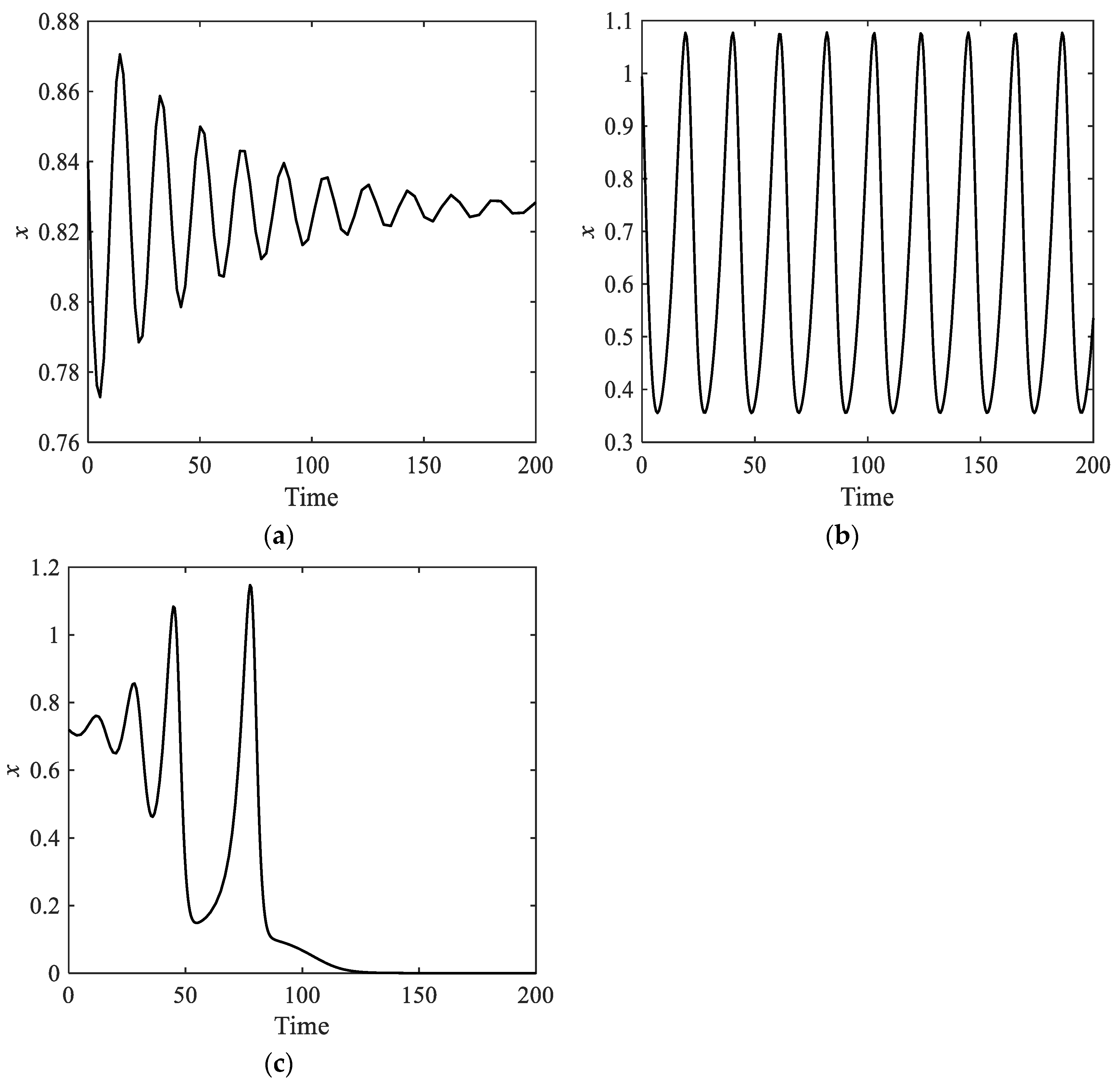
3.5. Robustness Discussion

To ensure the robustness of the results, we use two different sets of parameter values as shown in

Table 1. Typical parameter values of the model.

Parameter	Value 1	Value 2
${\beta }_1$	1.25	0.75
${\beta }_2$	1.0	0.5
${\alpha }_2$	6.0	4.0
$\delta$	0.25	0.25
$K$	2.0	2.0

for discussion and compare them with the original results. Due to space limitations, this paper only presents the influence of wage income changes on the potential market size of innovative products in scenarios where the impact of the distributive system on the dynamics of effective production capacity is insignificant. The results are shown in Figure 8. The parameters for Figure 8a,b correspond to the last two columns of Table 1, respectively. In Figure 8a, the initial value is at the steady state corresponding to ${\alpha }_1=2.5$, we analyze two directions: (1) at the initial moment, if ${\alpha }_1$ rises to 3, $x$ tends towards a lower steady state value (as indicated by the dashed line in the 0–200th period); then, at the 200th period, if ${\alpha }_1$ rises further to 3.5, $x$ tends towards the steady state value of 0 (as shown by the dashed line in the 200–300th period); (2) alternatively, at the initial time, $\mathrm{i}\mathrm{f}{\alpha }_1$ drops to 2.1,$x$ approaches a lower steady state value (as shown by the solid line in the 0–100th period); then, in the 100th period, ${\mathrm{i}\mathrm{f}\mathsf{\alpha }}_1$ decreases further to 1.4, $x$ approaches a cyclical solution (as indicated by the solid line in the 100–200 period); and finally, in the 200th period,$\mathrm{i}\mathrm{f}{\mathsf{\alpha }}_1$ decreases to 1, $x$ approaches the steady state value of 0. Similarly, Figure 8b exhibits the same dynamics, with the initial value at the steady state value corresponding to ${\alpha }_1=1.3$, rising sequentially to 1.75 and 2 in the first direction, and decreasing sequentially to 1.15, 0.9, and 0.5 in the second direction. The dynamic characteristics of $x$ under both sets of parameter values are consistent with those as shown in Figure 4b, indicating that the model has strong robustness.

4. Empirical Analysis

Based on the above model, two empirical analyses are conducted on the rise of the information technology industry and the consolidation and decline of neoliberal SSA under the economic long wave since the 1970s. Statistical tests and robustness checks are also performed.

4.1. The Rise of Information Technology Industry Under Economic Long Wave

The proportion of the added value of the information industry (PAVII) to GDP is used to express the development of the information technology industry in this paper (the data come from the United States Bureau of Economic Analysis: https://apps.bea.gov/, (accessed on 16 October 2024)). As shown in Figure 9, the profit rate (PR) is represented by the red dotted line (left axis), the blue solid line represents PAVII (right axis), and the shaded areas indicate the periods of economic recession. In the 1960s, PAVII grew slowly, with an increase of no more than 0.25 percentage points. From the mid-1970s to the mid-1980s, PAVII rapidly increased by over 0.85 percentage points. According to the timing of the U.S. economic recession and the change characteristics of PR in the corporate sector, the U.S. has experienced two economic recessions accompanied by declines in PR during rapid expansion of the information technology industry in the past decade. Specifically, in 1973, as the American economy began to decline, PR fell almost to its lowest level since the end of World War II, prompting PAVII to reverse its previous stagnation and increase rapidly; and from 1980 to 1982, another severe recession led to a continuous drop in PR, while PAVII grew even faster during this period and the following two years. We further find that, during and around this period, the significant decrease in PR clearly precedes the significant increase in PAVII. This temporal relationship suggests that the economic recession promoted the development of the information industry in the U.S., supporting the depression-induced theory. Moreover, the changes in PR also indicate that large-scale capital depreciation is a key factor in stimulating the rise of new industries.

In addition, the cointegration relationship between PR and PAVII is found to provide a more detailed analysis of the data, including statistical tests and robustness checks.

Table 2. ADF Unit Root Test Results.

Indicators	Test Form (C, T, P)	ADF Stats.	Critical Value	p-Value	Conclusion
PR	(0, 0, 11)	−0.674771	$-1.613799*$	0.421301	Nonstationary
ΔPR	(0, 0, 11)	−7.648102	$-2.598416***$	0.000000	Smoothness
PAVII	(C, T, 11)	−2.855417	$-3.164499*$	0.183189	Nonstationary
ΔPAVII	(C, 0, 11)	−8.981742	$-3.528514***$	0.000000	Smoothness
${\epsilon }_t$	(0, 0, 11)	−2.804014	$-1.945456 **$	0.0056	Smoothness

Note: *, **, and *** show levels of significance at 10%, 5%, and 1%.

presents the outcomes of augmented Dickey–Fuller (ADF) unit root tests. Herein, C and T denote the constant term and the time trend term, respectively, P denotes the lag order used, Δ represents the first-order difference, ${\mathsf{\epsilon }}_{\mathrm{t}}$ represents residual sequence. The critical values in the table are obtained from the data provided by Mackinnon. Values marked with * indicate critical values at a 10% significance level, those with ** denote critical values at a 5% significance level, and the rest with *** are critical values at a 1% significance level. It can be seen that the original variable series of PR and PAVII are nonstationary with a unit root, while the first-order difference series are stationary because the ADF test values of the original time series of PR and PAVII are greater than the corresponding critical value, whereas the ADF test values of the first-order difference series are less than the corresponding critical values, indicating that the original variable series of PR and PAVII are all I(1) series, which meet the requirements of conducting the cointegration analysis. The residual series ${\epsilon }_t$ is smooth.

The cointegration regression results of PR and PAVII are carried out by the ordinary least squares method. As shown in

Table 3. Cointegral Regression Results.

Variable	Coefficient	Std. Error	t-Statistic	p-Value
PR	−0.505038	0.046631	−10.83047	0.0000
C	2.842118	0.131229	21.65778	0.0000
R-squared	0.626266	Mean dependent var	1.426421
Adjusted R-squared	0.620927	S.D. dependent var	0.159964
S.E. of regression	0.098488	Akaike info criterion	−1.770382
Sum squared resid	0.678990	Schwarz criterion	−1.707141
Log likelihood	65.73376	Hannan–Quinn criter.	−1.745206
F-statistic	117.2991	Durbin–Watson stat	0.421299
Prob (F-statistic)	0.000000	-	-

, PR and PAVII have a cointegration relationship with a coefficient of −0.505038 and constant of 2.842118. The stationarity of residual sequences is tested.

Table 4. Results of the Granger Causality Test.

Null Hypothesis	Lag	F-Stats.	p-Value	Direction of Causality
PR $\ne$PAVII	2	3.280187	0.043936	PR$\leftrightarrow$PAVII
PAVII $\ne$PR	2	5.551236	0.005945

presents the results of a causal relationship between PR and PAVII, and it can be seen that there is a bidirectional Granger causality between them. The information industry also helps boost economic recovery and development. Therefore, the government should optimize science and technology innovation policies, improve the accuracy of support for enterprise research and development activities for encouraging enterprises to perform original technology innovation, fully implement research and development supporting funds, and implement certain tax reduction policies for rewarding technology innovation enterprises and individuals. The investment funds must be increased, with a focus on technology industries such as artificial intelligence and quantum communication to promote sustainable economic development.

4.2. The Consolidation and Decline of Neoliberal SSA

The SSA school believes that neoliberal SSA was established in the 1980s [39]. In fact, the development of emerging industries has laid the material foundation for the establishment of the new SSA. At the macro level, emerging industries dominated the long wave rise period, providing a relatively stable macro environment for the new institutional structure to operate; at the micro level, these industries improved the technological conditions necessary for establishing the new SSA. For example, with the help of information and communication technology, capital can freely flow on a wider scale, leading to spatial division and spatial redeployment of labor [40]. This process has promoted the formation of a “strong capital, weak labor” institutional structure, i.e., the most prominent feature of neoliberal SSA is the predominance of capital power over labor power. The proportion of total wages to net domestic product in the U.S. began to decline in 1970s, as shown in Figure 10a. By the early 1990s, the labor share in the U.S. had dropped below 54%, indicating a significant shift in the distributive institutional structure towards the interests of employers. What impact does this adjustment in institutional structure have on the economic cycle? We use actual GDP data of the U.S. for analysis. It should be noted that the economic cycle model in this article seems to be quite different from the real economic cycle. In fact, the former is the result of a specific reference frame, where the real economic aggregate continues to rise, while the model constructed in this article is a limited growth model. A Hodrick–Prescott filter (HP) is used to extract long-term characteristics [41]. In order to compare the economic cycle in the model with the real economic cycle, an HP filter is performed on the real GDP of the U.S. from 1991 to 2009. Figure 10b shows the fluctuation of the real GDP. It can be observed that the actual economic cycle characteristics of the U.S. during this period are very similar to those depicted in Figure 7c: initially, economic fluctuations are small, then they increase, and finally, they tend to collapse. Figure 10c,d further present the phase trajectory and actual output dynamics of the system, respectively. In this case, the initial point of the dynamical system is located near the equilibrium point ${\mathrm{S}}_3$, and after a period of oscillation, it “brushes past” the equilibrium point ${\mathrm{S}}_2$ and eventually converges to the equilibrium point ${\mathrm{S}}_1$.

In the above model, this cyclical feature is precisely caused by the excessive inclination of the distributive institutional structure towards the capital interests. In fact, in the early 1990s, the U.S. economy returned to a balanced state after a brief recession. Due to the strong power of capital, the profitability of capital quickly recovered, the speed of capital accumulation accelerated, and information technology was widely applied, resulting in high employment, high growth, and low inflation coexisting. During this period, neoliberal SSA gradually consolidated its economy. There is a hidden risk of excessive capital accumulation behind the new economic prosperity. Around 2000, the economic imbalance caused by excessive capital accumulation reached its peak, and the overproduction crisis triggered by the bursting of the technology stock bubble broke out. This brief economic recession cleared some excess capacity, paving the way for an economic expansion from 2002 to 2007. Since the institutional structure of “strong capital and weak labor” did not change, profit margins recovered strongly and reached the highest levels recorded since the 1980s. The recovery in profit margin signified a renewed capital accumulation rate, and the process of excessive capital accumulation resumed, eventually culminating in the overproduction economic crisis of 2008. The financial crisis that erupted in the U.S. and spread rapidly around the world marked the decline of neoliberal SSA.

5. Conclusions

This paper focuses on the explanation of the agents of economic long waves from the perspectives of technology and institutions. It explores the laws of limited growth in technological innovation and value realization by constructing nonlinear interaction and nonequilibrium evolution models. On this basis, the relationships between endogenous technological innovation, institutional regulation, and economic long waves are explored. The main conclusions are as follows.

Firstly, the free markets exhibit the possibility of endogenous instability, that is, regulating production through the interaction of supply and demand does not necessarily lead to equilibrium. This instability stems from positive feedback effects induced by mechanisms such as demand renewal, social contagion, and consumer psychology.

Secondly, technological innovation plays a fundamental role in the economic long wave movement, and it is itself driven by the capital accumulation associated with the economic long wave. The basic innovation, improved innovation, and breakthrough innovation spurred by productive institutional regulation together constitute the driving force behind the upward phase of the long wave.

Thirdly, through the dual regulation of productive and distributive institutions, it is possible to ensure stable and efficient economic development while also securing broad social benefits. However, under the condition of individual decentralized decision making, institutional structures often deviate from this optimal outcome, and such deviations can lead to structural economic crises.

Finally, this investigation indicates the integration and interaction of technological innovation and institutional regulation jointly drive the long wave movement and accumulation cycle of the economy. This paper provides a practical and feasible method for researching economic long waves to promote sustainable and sound economic development.

Although this article enriches and expands the theory of economic long waves, there remain issues that warrant further exploration. Since the 1970s, financialization has become an increasingly significant characteristic of the contemporary capitalist economy. The interaction between production capital and financial capital is an important feature of economic long wave movement. However, the long wave model presented in this article neglects the dynamics of financial capital, which is a limitation of this article. Investigating the interaction mechanism between productive and financial capital and its implications for long wave movements will be the focus of our future research.

References

1. Kondratiev, N.D. The long waves in economic life. Rev. Econ. Stat. 1935, 17, 105–115. [Google Scholar] [CrossRef]
2. Day, R. The theory of the long cycle: Kondratiev, Trotsky, Mandel. New Left Rev. 1976, 99, 67–82. [Google Scholar]
3. Forrester, J.W. Business structure, economic cycles, and national policy. Futures 1976, 8, 195–214. [Google Scholar] [CrossRef]
4. Schumpeter, J.A. Business Cycles: A Theoretical, Historical and Statistical Analysis of the Capitalist Process; McGraw-HIll: New York, NY, USA, 1939. [Google Scholar]
5. Volland, C.S. A comprehensive theory of long wave cycles. Technol. Forecast. Soc. 1987, 32, 123–145. [Google Scholar] [CrossRef]
6. Forrester, J.W. Innovation and the economic long wave. Plan. Rev. 1980, 8, 6–15. [Google Scholar] [CrossRef]
7. Rosenberg, N.; Frischtak, C.R. Long waves and economic growth: A critical appraisal. Am. Econ. Rev. 1983, 73, 146–151. [Google Scholar]
8. Coombs, R.W. Innovation, automation and the long-wave theory. Futures 1981, 13, 360–370. [Google Scholar] [CrossRef]
9. Devezas, T.C.; Linstone, H.A.; Santos, H.J.S. The growth dynamics of the Internet and the long wave theory. Technol. Forecast. Soc. 2005, 72, 913–935. [Google Scholar] [CrossRef]
10. Coccia, M. The Source and Nature of General Purpose Technologies for Supporting Next K-Waves: Global Leadership and the Case Study of the U.S. Navy’s Mobile User Objective System. Technol. Forecast. Soc. 2017, 116, 331–339. [Google Scholar] [CrossRef]
11. Kotz, D.M.; McDonough, T.; Reich, M. Social Structures of Accumulation-The Political Economy of Growth and Crisis; Cambridge University Press: Cambridge, UK, 1944. [Google Scholar]
12. Boyer, R. The Regulation School: A Critical Introduction; Columbia University Press: New York, NY, USA, 1990. [Google Scholar]
13. Jessop, B. Survey article: The regulation approach. J. Polit. Philos. 1997, 5, 287–326. [Google Scholar] [CrossRef]
14. Papenhausen, C. A cyclical model of institutional change. Foresight 2009, 11, 4–13. [Google Scholar] [CrossRef]
15. Mandel, E. Long Waves of Capitalist Development: A Marxist Interpretation; Verso: London, UK, 1995. [Google Scholar]
16. Menshikov, S. The long wave as an endogenous mechanism. In New Findings in Long-Wave Research; Palgrave Macmillan UK: London, UK, 1992. [Google Scholar]
17. Rostow, W.W. The World Economy: History & Prospect; University of Texas press: Austin, TX, USA, 1978. [Google Scholar]
18. Mensch, G. Stalemate in Technology; Ballinger: Cambridge, MA, USA, 1979. [Google Scholar]
19. Van Duijn, J.J. The Long Wave in Economic Life; George Allen and Unwin: London, UK, 1983. [Google Scholar]
20. Schmookler, J. Invention and Economic Growth; Harvard University Press: Cambridge, MA, USA, 1966. [Google Scholar]
21. Gordon, D.M.; Edwards, R.; Reich, M. Segmented Work, Divided Workers: The Historical Transformantion of Labor in the United States; Cambridge University Press: Cambridge, UK, 1982. [Google Scholar]
22. Wolfson, M.H.; Kotz, D. A reconceptualization of social structure of accumulation theory. World Rev. Polit. Econ. 2010, 1, 209–225. [Google Scholar]
23. Perez, C. Technological Revolutions and Financial Capital: The Dynamics of Bubbles and Golden Ages; Edward Elgar Publishing: Cheltenham, UK, 2002. [Google Scholar]
24. Arthur, W.B. The Economy as an Evolving Complex System II; CRC Press: Boca Raton, FL, USA, 2018. [Google Scholar]
25. Arthur, W.B. Foundations of complexity economics. Nat. Rev. Phys. 2021, 3, 136–145. [Google Scholar] [CrossRef]
26. Uehara, T.; Cordier, M.; Hamaide, B. Fully dynamic input-output/system dynamics modeling for ecological-economic system analysis. Sustainability 2018, 10, 1765. [Google Scholar] [CrossRef]
27. Jahanshahi, H.; Sajjadi, S.S.; Bekiros, S.; Aly, A.A. On the development of variable-order fractional hyperchaotic economic system with a nonlinear model predictive controller. Chaos Soliton Fract. 2021, 144, 110698. [Google Scholar] [CrossRef]
28. Bischi, G.I. From Samuelson’s multiplier-accelerator to bifurcations and chaos in economic dynamics. Decis. Econ. Financ. 2024, 1–22. [Google Scholar] [CrossRef]
29. Chen, P. Biophysical limit and metabolic growth: New understanding of modern division of labor and sustainable economies. Real-World Econ. Rev. 2023, 106, 93–105. [Google Scholar]
30. Semmler, W.; Della Rossa, F.; Orlando, G.; Rosario, G.R.; Koçkesen, L. Endogenous economic resilience, loss of resilience, persistent cycles, multiple attractors, and disruptive contractions. In Multiplicity of Time Scales in Complex Systems: Challenges for Sciences and Communication II; Springer Nature Switzerland: Cham, Switzerland, 2023; pp. 259–306. [Google Scholar]
31. Parui, P. Fiscal expansion, government debt and economic growth: A post-Keynesian perspective. J. Post Keynes. Ec. 2024, 47, 117–154. [Google Scholar] [CrossRef]
32. Chen, P. Metabolic growth theory: Market-share competition, learning uncertainty, and technology wavelets. J. Evol. Econ. 2014, 24, 239–262. [Google Scholar] [CrossRef]
33. Mulder, P.; De Groot, H.L.F.; Hofkes, M.W. Economic growth and technological change: A comparison of insights from a neo-classical and an evolutionary perspective. Technol. Forecast Soc. 2001, 68, 151–171. [Google Scholar] [CrossRef]
34. Hsu, S.B.; Che, K.C. Ordinary Differential Equations with Applications; World Scientific: Singapore, 2013. [Google Scholar]
35. Boi, L. Geometry of dynamical systems and topological stability: From bifurcation, chaos and fractals to dynamics in natural and life sciences. Int. J Bifurc. Chaos 2011, 21, 815–867. [Google Scholar] [CrossRef]
36. Rasmussen, S.; Mosekilde, E.; Sterman, J.D. Bifurcations and chaotic behavior in a simple model of the economic long wave. Syst. Dynam. Rev. 1985, 1, 92–110. [Google Scholar] [CrossRef]
37. Boddy, R.; Crotty, J. Class conflict, Keynesian policies, and the business cycle. Mon. Rev. 1974, 26, 1–19. [Google Scholar] [CrossRef] [PubMed]
38. Kotz, D.M. The Financial and Economic Crisis of 2008: A Systemic Crisis of Neoliberal Capitalism. Rev. Radical Pol. Econ. 2009, 41, 305–317. [Google Scholar] [CrossRef]
39. Kotz, D.M.; McDonough, T. Global neoliberalism and the contemporary social structure of accumulation. In Contemporary Capitalism and Its Crises: Social Structure of Accumulation Theory for the 21st Century; McDonough, T., Reich, M., Kotz, D.M., Eds.; Cambridge University Press: New York, NY, USA, 2010; pp. 93–120. [Google Scholar]
40. Wallace, M.; Brady, D. Globalization or spatialization? The worldwide spatial restructuring of the labor process. In Contemporary Capitalism and Its crises: Social Structure of Accumulation Theory for the 21st Century; McDonough, T., Reich, M., Kotz, D.M., Eds.; Cambridge University Press: New York, NY, USA, 2010; pp. 121–144. [Google Scholar]
41. De Jong, R.M.; Sakarya, N. The econometrics of the Hodrick-Prescott filter. Rev. Econ. Stat. 2016, 98, 310–317. [Google Scholar] [CrossRef]
Figure 1. Correlation diagram of long wave model. (a) Four equilibrium solutions; (b) Three equilibrium solutions.
Sustainability 17 02758 g001
Figure 2. Bifurcation diagram and output change of basic innovation caused by depression. (a) Bifurcation diagram; (b) Output change.
Sustainability 17 02758 g002
Figure 3. Bifurcation diagram of potential market size.
Sustainability 17 02758 g003
Figure 4. Bifurcation diagram of institution regulation. (a) Productive institution; (b) Distributive institution.
Sustainability 17 02758 g004
Figure 5. Distributive institutional regulation.
Sustainability 17 02758 g005
Figure 6. Optimal institutional structure.
Sustainability 17 02758 g006
Figure 7. Different periodic fluctuations. (a) α 1 = 0.6 ; (b) α 1 = 0.5 ; (c) α 1 = 0.42 .
Sustainability 17 02758 g007
Figure 8. Robustness analysis of distributive institution. (a) Value 1; (b) Value 2.
Sustainability 17 02758 g008
Figure 9. Proportion of added value of information industry (right axis) and profit rate (left axis).
Sustainability 17 02758 g009
Figure 10. (a) Trends of American labor share; (b) Real GDP fluctuations in U.S.; (c) System phase trajectory diagram; (d) Output dynamics in the model.
Sustainability 17 02758 g010