Collaboration and Resource Sharing for the Multi-Depot Electric Vehicle Routing Problem with Time Windows and Dynamic Customer Demands


Abstract

1. Introduction
2. Literature Review
2.1. Electric Vehicle Routing Problem with Dynamic Customer Demand
2.2. Multi-Depot Electric Vehicle Routing Problem
2.3. Collaborative and Resource Sharing
2.4. Relevant Solution Methods
3. Problem Statement
4. Related Definitions and Model Formulation
4.1. Solution Methodology
4.2. Model Formulation
5. Solution Methodology
5.1. Mini-Batch k-Means Clustering
| Algorithm 1: mini-batch k-means |
| Input: time windows and geographical locations of customers and depots, and the number of clustering units k Output: multiple clustering units |
 |
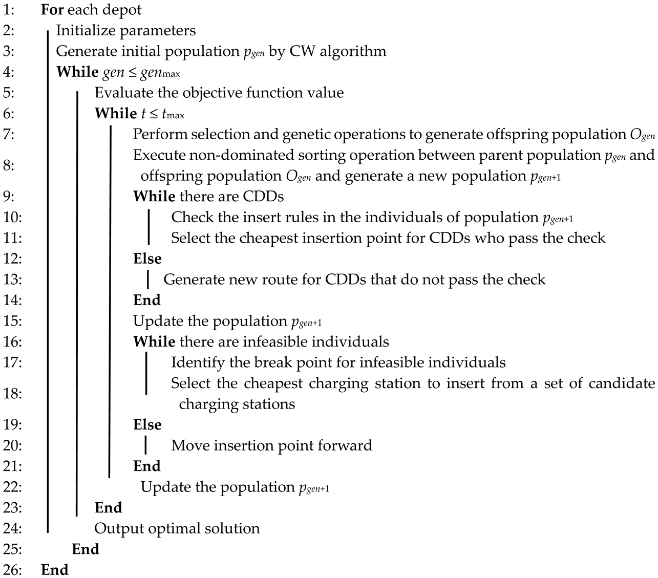
5.2. Improved Multi-Objective Differential Evolution
| Algorithm 2: IMODA algorithm |
| Input: parameters of algorithm (e.g., population size, maximum iterations, crossover probability, mutation probability); parameters of model; clustering results Output: optimal solution |
 |
5.2.1. Initiation Population
5.2.2. Genetic Operation
- (1)
- Mutation operation
- (2)
- Crossover operation
- (3)
- Selection operation
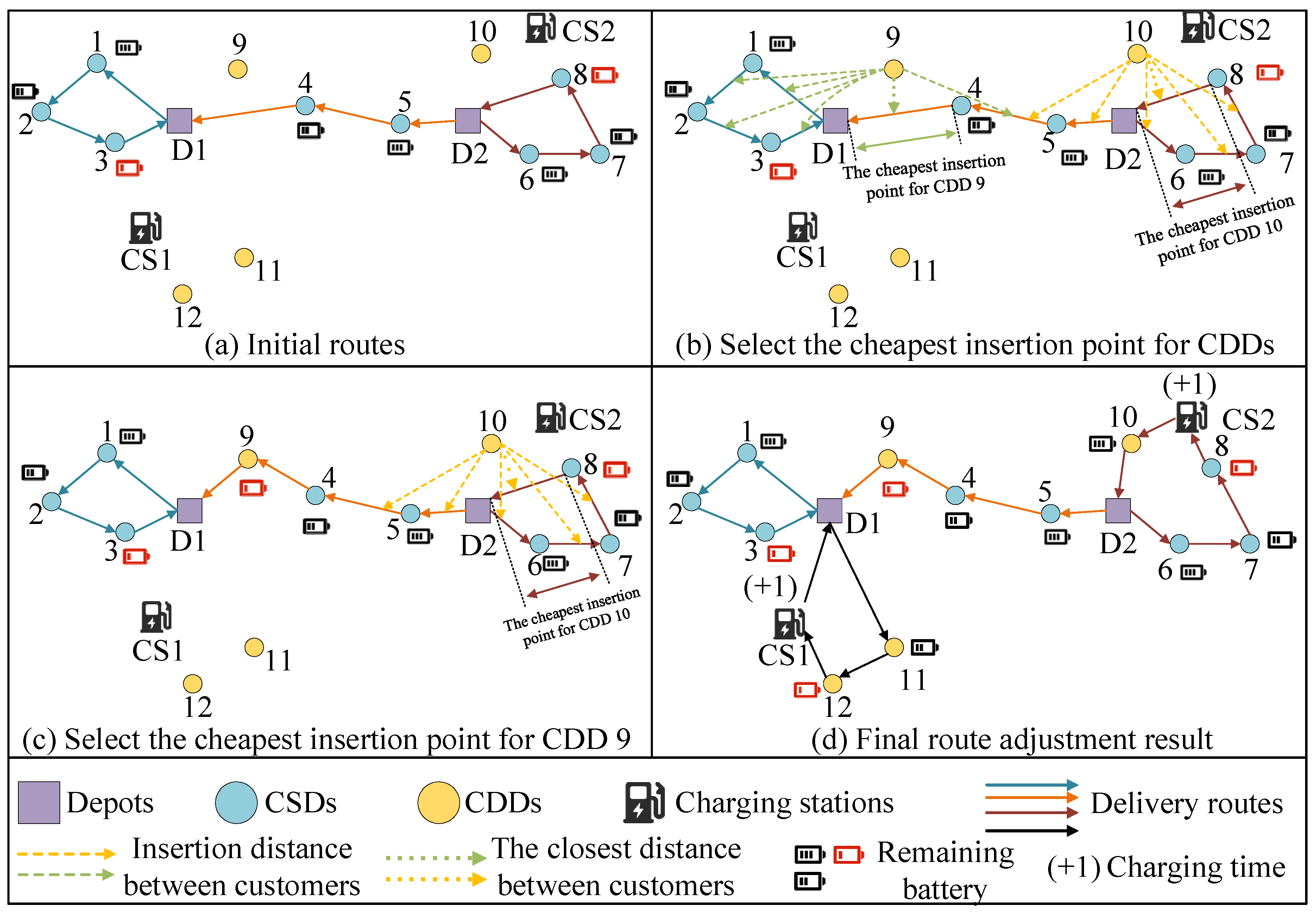
5.2.3. Dynamic Customer Insertion Strategy
| Algorithm 3: CDD insertion operation |
| Input: population pgen+1 containing all CSDs, and information on the time windows and geographic locations of CDDs. Output: updated pgen+1 containing CSDs and CDDs |
 |
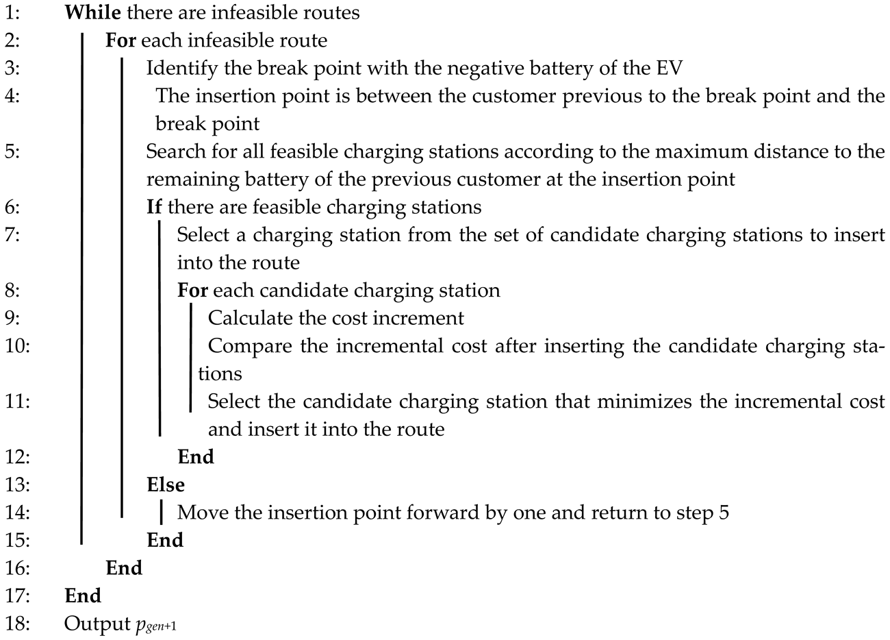
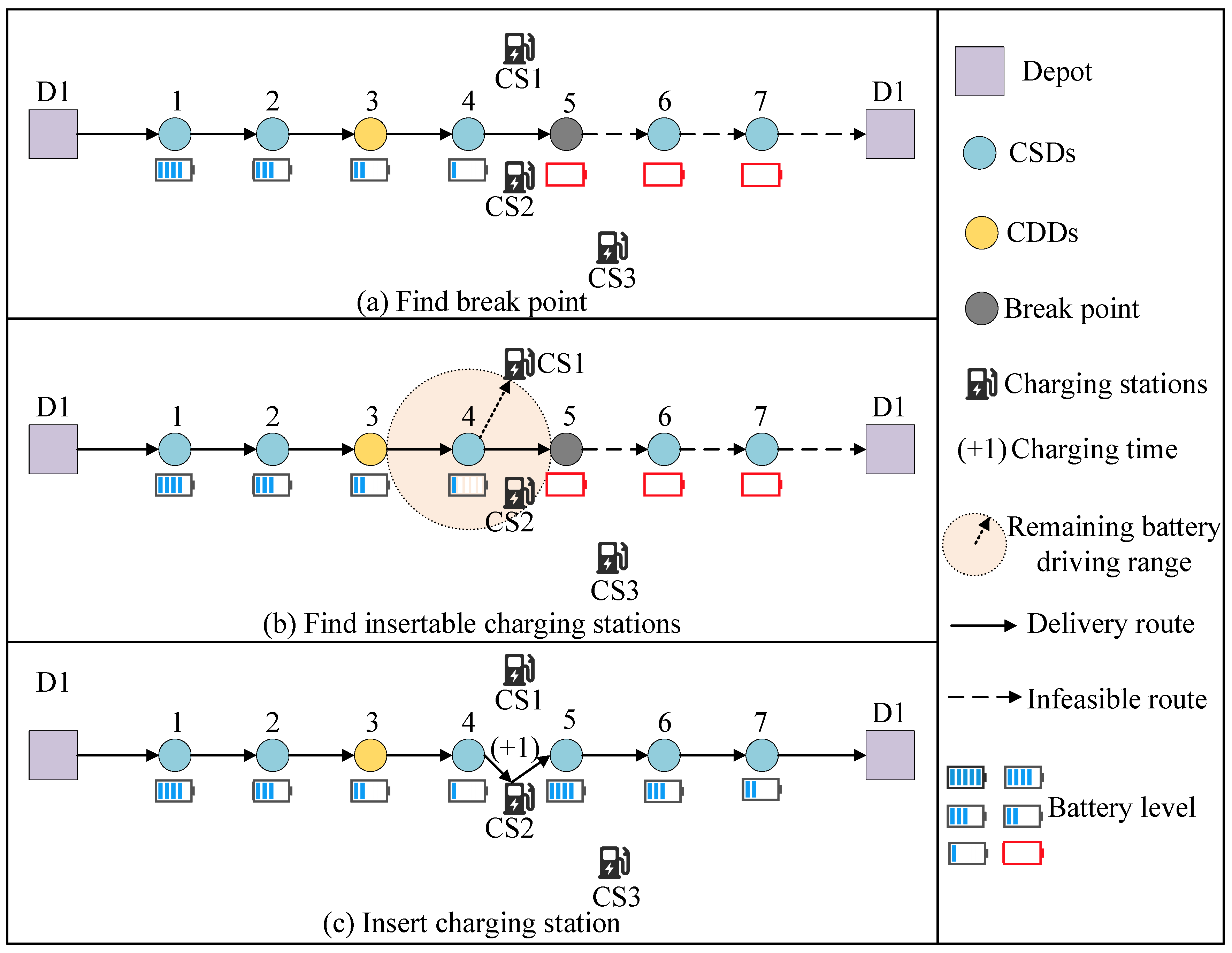
5.2.4. Charging Station Insertion Strategy
| Algorithm 4: the process of charging station insertion strategy |
| Input: population pgen+1, the geographic location of charging stations Output: updated pgen+1 |
 |
5.2.5. Non-Dominated Sorting Operation
6. Computational Experiments
6.1. Algorithm Comparison
6.2. Date Description and Related Parameter Setting
6.3. Optimization Results
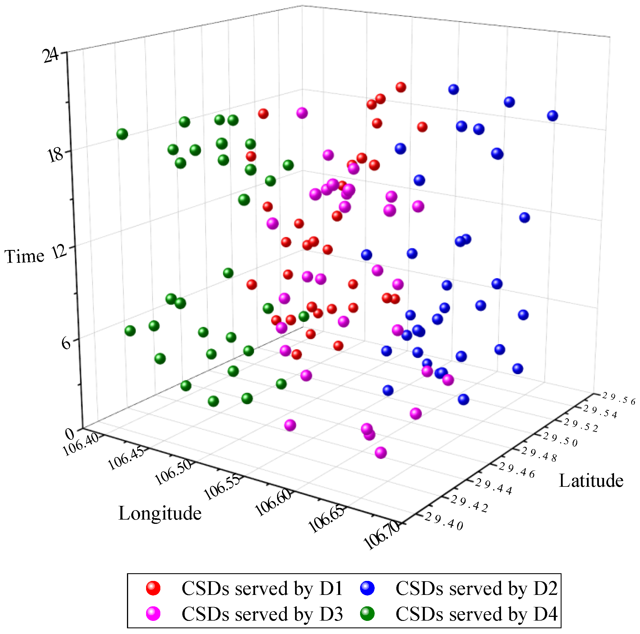
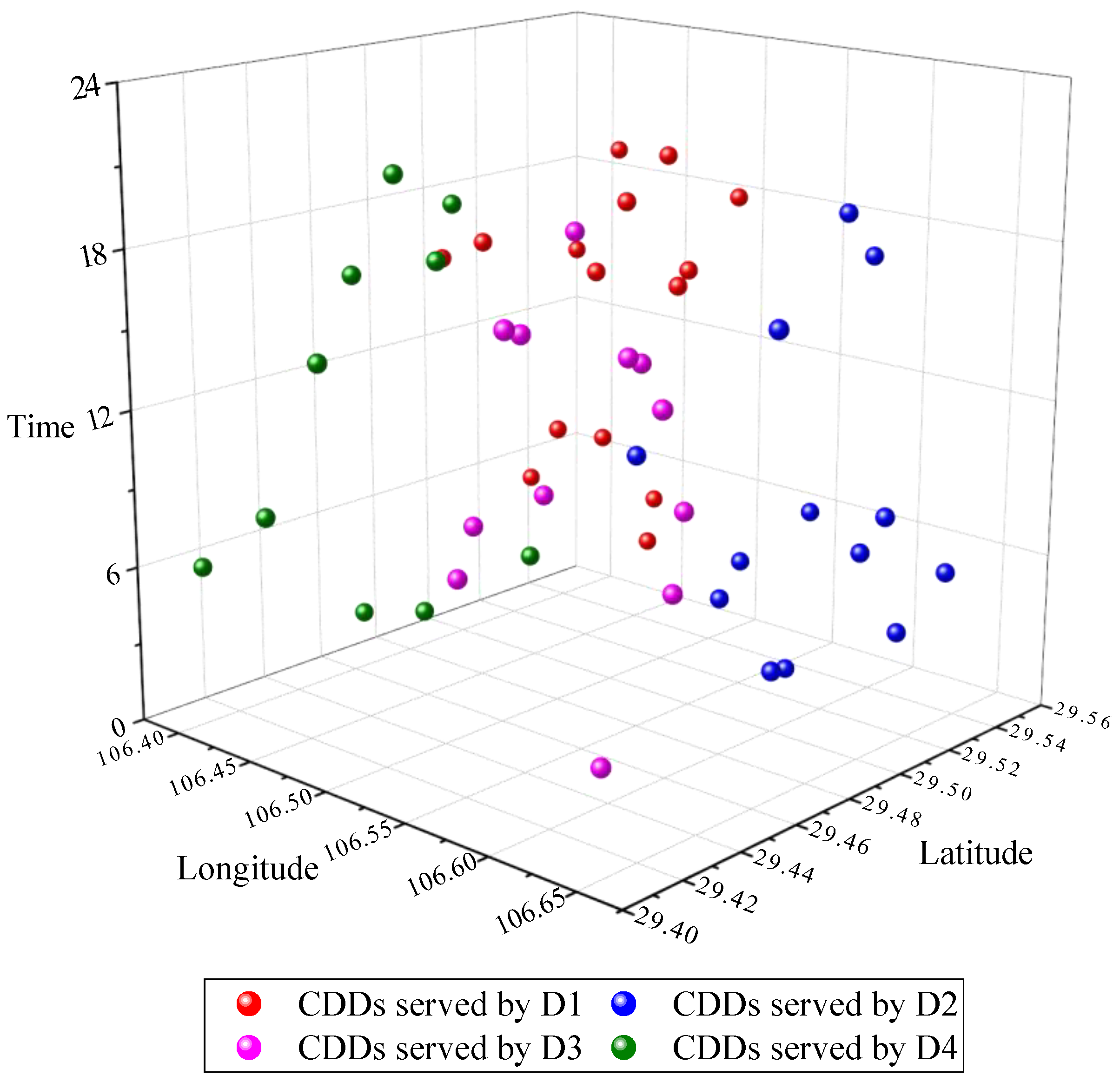
6.3.1. Clustering Results
6.3.2. Electric Vehicle Routing Optimization with Resource Sharing and Insertion Strategy
6.4. Analysis and Discussion
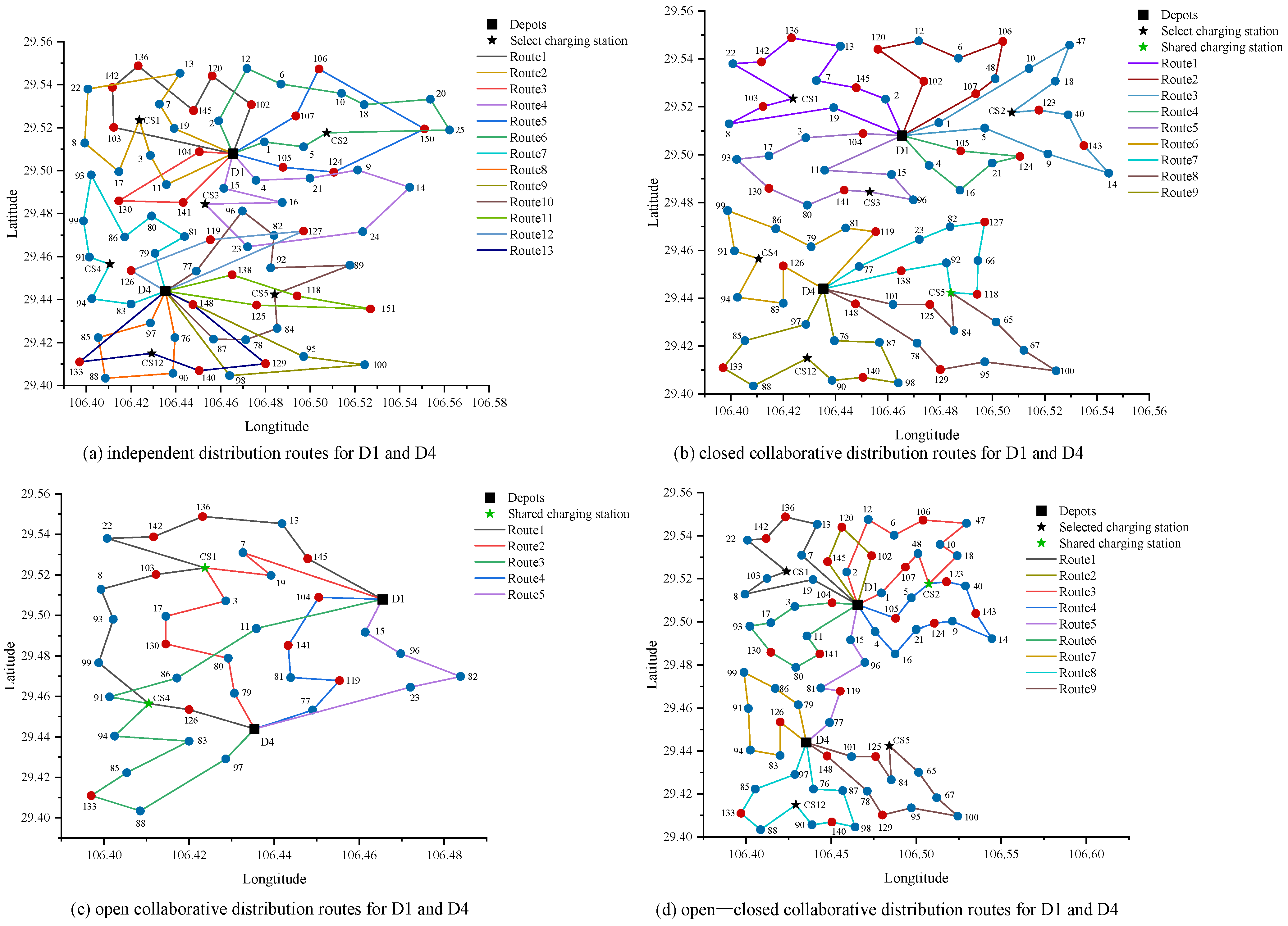
6.4.1. Comparison of Different Strategies for CDDs
6.4.2. Comparison of Different Delivery Modes
7. Conclusions
Author Contributions
Funding
Institutional Review Board Statement
Informed Consent Statement
Data Availability Statement
Conflicts of Interest
References
- Allahyari, S.; Yaghoubi, S.; Van Woensel, T. The secure time-dependent vehicle routing problem with uncertain demands. Comput. Oper. Res. 2021, 131, 105253. [Google Scholar] [CrossRef]
- Wang, S.; Sun, W.; Huang, M. An adaptive large neighborhood search for the multi-depot dynamic vehicle routing problem with time windows. Comput. Ind. Eng. 2024, 191, 110122. [Google Scholar] [CrossRef]
- Jiang, Y.; Hu, W.; Gu, W.; Yu, Y.; Xu, M. A multi-mode hybrid electric vehicle routing problem with time windows. Transportation Res. Part E Logist. Transp. Rev. 2025, 195, 103976. [Google Scholar] [CrossRef]
- Wang, Y.; Zhe, J.Y.; Wang, X.W.; Sun, Y.Y.; Wang, H. Z Collaborative multidepot vehicle routing problem with dynamic customer demands and time windows. Sustainability 2022, 14, 6709. [Google Scholar] [CrossRef]
- Basso, R.; Kulcsár, B.; Sanchez-Diza, I.; Qu, X.B. Dynamic stochastic electric vehicle routing with safe reinforcement learning. Transp. Res. Part E Logist. Transp. Rev. 2022, 157, 102496. [Google Scholar] [CrossRef]
- Macioszek, E. E-mobility infrastructure in the Górnośląsko-Zagłębiowska Metropolis, Poland, and potential for development. In Proceedings of the 5th World Congress on New Technologies, Lisbon, Portugal, 18–20 August 2019. [Google Scholar]
- Dong, J.T.; Wang, H.F.; Zhang, S.Z. Dynamic electric vehicle routing problem considering mid-route recharging and new demand arrival using an improved memetic algorithm. Sustain. Energy Technol. Assess. 2023, 58, 103366. [Google Scholar] [CrossRef]
- Li, J.X.; Liu, R.C.; Wang, R.N. Handling dynamic capacitated vehicle routing problems based on adaptive genetic algorithm with elastic strategy. Swarm Evol. Comput. 2024, 86, 101529. [Google Scholar] [CrossRef]
- Alvarez, A.; Cordeau, J.F.; Jans, R. The consistent vehicle routing problem with stochastic customers and demands. Transp. Res. Part B Methodol. 2024, 186, 102968. [Google Scholar] [CrossRef]
- Cacho EM, A.; Mangini, A.M.; Roccotelli, M.; Fanti, M.P. Electric vehicle routing optimization for postal delivery and waste collection in smart cities. IEEE Trans. Intell. Transp. Syst. 2025, 26, 3307–3323. [Google Scholar]
- Lu, J.; Chen, Y.; Hao, J.K.; He, R. The time-dependent electric vehicle routing problem: Model and solution. Expert Syst. Appl. 2020, 161, 113593. [Google Scholar] [CrossRef]
- Wang, Y.; Zhou, J.X.; Sun, Y.Y.; Fan, J.X.; Wang, Z.; Wang, H.Z. Collaborative multidepot electric vehicle routing problem with time windows and shared charging stations. Expert Syst. Appl. 2023, 219, 119654. [Google Scholar] [CrossRef]
- Karimpour, A.; Setak, M.; Hemmati, A. Estimating energy consumption and charging duration of electric vehicle in multigraph. Comput. Oper. Res. 2023, 155, 106216. [Google Scholar] [CrossRef]
- Gkiotsalitis, K.; Iliopoulou, C.; Kepaptsoglou, K. An exact approach for the multi-depot electric bus scheduling problem with time windows. Eur. J. Oper. Res. 2023, 306, 189–206. [Google Scholar] [CrossRef]
- Li, X.R.; Wang, W.; Gu, H. Redesign of sharing charging system for electric vehicles using blockchain technology. J. Clean. Prod. 2023, 415, 137775. [Google Scholar] [CrossRef]
- Agrali, C.; Lee, S. The multi-depot pickup and delivery problem with capacitated electric vehicles transfers, and time windows. Comput. Ind. Eng. 2023, 179, 109207. [Google Scholar] [CrossRef]
- Zhang, S.; Zhou, T.; Fang, C.; Yang, S.H. A novel collaborative electric vehicle routing problem with multiple prioritized time windows and time-dependent hybrid recharging. Expert Syst. Appl. 2024, 244, 122990. [Google Scholar] [CrossRef]
- Lu, C.C.; Yan, S.Y.; Li, H.C.; Diabat, A.; Wang, H.T. Optimal fleet deployment for electric vehicle sharing systems with the consideration of demand uncertainty. Comput. Oper. Res. 2021, 135, 105437. [Google Scholar] [CrossRef]
- Mancini, S.; Gansterer, M.; Hartl, R.F. The collaborative consistent vehicle routing problem with workload balance. Eur. J. Oper. Res. 2021, 293, 955–965. [Google Scholar] [CrossRef]
- Sarbijan, M.S.; Behnamian, J. Real-time collaborative feeder vehicle routing problem with flexible time windows. Swarm Evol. Comput. 2022, 75, 101201. [Google Scholar] [CrossRef]
- Ahari, S.A.; Bakir, I.; Roodbergen, K.J. A new perspective on carrier collaboration: Collaborative vehicle utilization. Transp. Res. Part C Emerg. Technol. 2024, 163, 104647. [Google Scholar] [CrossRef]
- Zhang, S.; Gajpal, Y.; Appadoo, S.S.; Abdulkader MM, S. Electric vehicle routing problem with recharging stations for minimizing energy consumption. Int. J. Prod. Econ. 2018, 203, 404–413. [Google Scholar] [CrossRef]
- Pelletier, S.; Jabali, O.; Laporte, G. The electric vehicle routing problem with energy consumption uncertainty. Transp. Res. Part B Methodol. 2019, 126, 225–255. [Google Scholar] [CrossRef]
- Comert, S.E.; Yazgan, H.R. A new approach based on hybrid ant colony optimization-artificial bee colony algorithm for multi-objective electric vehicle routing problems. Eng. Appl. Artif. Intell. 2023, 123, 106375. [Google Scholar] [CrossRef]
- Shen, Y.; Wu, J.; Ma, M.; Du, X.; Wu, H.; Fei, X.; Niu, D. Improved differential evolution algorithm based on cooperative multi-population. Eng. Appl. Artif. Intell. 2024, 133, 108149. [Google Scholar] [CrossRef]
- Li, M.; Zhao, Y.; Cao, R.; Wang, J.; Wu, D. A recursive framework for improving the performance of multi-objective differential evolution algorithms for gene selection. Swarm Evol. Comput. 2024, 87, 101546. [Google Scholar] [CrossRef]
- Wang, Y.; Yu, X.; Zhang, W. An improved reinforcement learning-based differential evolution algorithm for combined economic and emission dispatch problems. Eng. Appl. Artif. Intell. 2025, 140, 109709. [Google Scholar] [CrossRef]
- Wu, H.; Pang GK, H.; Choy, K.L.; Lam, H.Y. An optimization model for electric vehicle battery charging at a battery swapping station. IEEE Trans. Veh. Technol. 2017, 67, 881–895. [Google Scholar] [CrossRef]
- Liu, W.L.; Gong, Y.J.; Chen, W.N.; Liu, Z.; Wang, H.; Zhang, J. Coordinated charging scheduling of electric vehicles: A mixed-variable differential evolution approach. IEEE Trans. Intell. Transp. Syst. 2019, 21, 5094–5109. [Google Scholar] [CrossRef]
- Sethanan, K.; Jamrus, T. Hybrid differential evolution algorithm and genetic operator for multi-trip vehicle routing problem with backhauls and heterogeneous fleet in the beverage logistics industry. Comput. Ind. Eng. 2020, 146, 106571. [Google Scholar] [CrossRef]
- Souza, I.P.; Boeres MC, S.; Moraes RE, N. A robust algorithm based on differential evolution with local search for the capacitated vehicle routing problem. Swarm Evol. Comput. 2023, 77, 101245. [Google Scholar] [CrossRef]
- Shao, S.; Guan, W.; Bi, J. Electric vehicle-routing problem with charging demands and energy consumption. IET Intell. Transp. Syst. 2018, 12, 202–212. [Google Scholar] [CrossRef]
- Shen, Y.; Yu, L.; Li, J. Robust electric vehicle routing problem with time windows under demand uncertainty and weight-related energy consumption. Complex Syst. Model. Simul. 2022, 2, 18–34. [Google Scholar] [CrossRef]
- Lera-Romero, G.; Bront JJ, M.; Soulignac, F.J. A branch-cut-and-price algorithm for the time-dependent electric vehicle routing problem with time windows. Eur. J. Oper. Res. 2024, 312, 978–995. [Google Scholar] [CrossRef]
- Li, H.; Li, Z.; Cao, L.; Wang, R.; Ren, M. Research on optimization of electric vehicle routing problem with time window. IEEE Access 2020, 8, 146707–146718. [Google Scholar] [CrossRef]
- Asghari, M.; Al-e SM, J.M. Green vehicle routing problem: A state-of-the-art review. Int. J. Prod. Econ. 2021, 231, 107899. [Google Scholar] [CrossRef]
- Zeng, Z.; Zhang, M.; Chen, T.; Hong, Z. A new selection operator for differential evolution algorithm. Knowl.-Based Syst. 2021, 226, 107150. [Google Scholar] [CrossRef]
- Alesiani, F.; Ermis, G.; Gkiotsalitis, K. Constrained clustering for the capacitated vehicle routing problem. Appl. Artif. Intell. 2022, 36, 1995658. [Google Scholar] [CrossRef]
- Ahmed, M.A.; Baharin, H.; Nohuddin PN, E. Mini-batch k-means versus k-means to cluster english tafseer text: View of Al-Baqarah chapter. J. Quranic Sci. Res. 2021, 2, 48–53. [Google Scholar] [CrossRef]
- Han, X.; Wang, Z.; Xu, H.J. Time-weighted collaborative filtering algorithm based on improved mini batch K-means clustering. Adv. Sci. Technol. 2021, 105, 309–317. [Google Scholar]
- Kunnapapdeelert, S.; Klinsrisuk, R. Determination of green vehicle routing problem via differential evolution. Int. J. Logist. Syst. Manag. 2019, 34, 395–410. [Google Scholar] [CrossRef]
- Wang, Y.; Wei, Y.H.; Wang, X.W.; Wang, Z.; Wang, H.Z. A clustering-based extended genetic algorithm for the multidepot vehicle routing problem with time windows and three-dimensional loading constraints. Appl. Soft Comput. 2023, 133, 109922. [Google Scholar] [CrossRef]
- Wei, Y.H.; Wang, Y.; Hu, X.P. The two-echelon truck-unmanned ground vehicle routing problem with time-dependent travel times. Transp. Res. Part E Logist. Transp. Rev. 2025, 194, 103954. [Google Scholar] [CrossRef]
- Sankul, S.; Supattananon, N.; Akararungruangkul, R.; Wichapa, N. An adaptive differential evolution algorithm to solve the multi-compartment vehicle routing problem: A case of cold chain transportation problem. Int. J. Prod. Manag. Eng. 2024, 12, 91–104. [Google Scholar] [CrossRef]
- Ming, Y.L.; Erbao, C. An improved differential evolution algorithm for vehicle routing problem with simultaneous pickups and deliveries and time windows. Eng. Appl. Artif. Intell. 2010, 23, 188–195. [Google Scholar] [CrossRef]
- Moonsri, K.; Sethanan, K.; Worasan, K.; Nitisiri, K. A hybrid and self-adaptive differential evolution algorithm for the multi-depot vehicle routing problem in egg distribution. Appl. Sci. 2021, 12, 35. [Google Scholar] [CrossRef]
- Malik, S.; Kim, D.H. Optimal travel route recommendation mechanism based on neural networks and particle swarm optimization for efficient tourism using tourist vehicular data. Sustainability 2019, 11, 3357. [Google Scholar] [CrossRef]
- Ge, X.; Zhu, Z.; Jin, Y. Electric vehicle routing problems with stochastic demands and dynamic remedial measures. Math. Probl. Eng. 2020, 2020, 8795284. [Google Scholar] [CrossRef]
- Archetti, C.; Guerriero, F.; Macrina, G. The online vehicle routing problem with occasional drivers. Comput. Oper. Res. 2021, 127, 105144. [Google Scholar] [CrossRef]
- Chen, S.; Chen, R.; Wang, G.G.; Gao, J.; Sangaiah, A.K. An adaptive large neighborhood search heuristic for dynamic vehicle routing problems. Comput. Electr. Eng. 2018, 67, 596–607. [Google Scholar] [CrossRef]
- Montoya, A.; Guéret, C.; Mendoza, J.E.; Villegas, J.G. The electric vehicle routing problem with nonlinear charging function. Transp. Res. Part B Methodol. 2017, 103, 87–110. [Google Scholar] [CrossRef]
- Wang, Y.; Gou, M.Y.; Luo, S.Y.; Fan, J.X.; Wang, H.Z. The multi-depot pickup and delivery vehicle routing problem with time windows and dynamic demands. Eng. Appl. Artif. Intell. 2025, 139, 109700. [Google Scholar] [CrossRef]
- Wang, Y.; Yuan, Y.Y.; Guan, X.Y.; Wang, H.Z.; Liu, Y.; Xu, M.Z. Collaborative mechanism for pickup and delivery problems with heterogeneous vehicles under time windows. Sustainability 2019, 11, 3492. [Google Scholar] [CrossRef]
- Zhao, P.X.; Luo, W.H.; Han, X. Time-dependent and bi-objective vehicle routing problem with time windows. Adv. Prod. Eng. Manag. 2019, 14, 201–212. [Google Scholar] [CrossRef]
- Guezouli, L.; Abdelhamid, S. Multi-objective optimization using genetic algorithm based clustering for multi-depot heterogeneous fleet vehicle routing problem with time windows. Int. J. Math. Oper. Res. 2018, 13, 332–349. [Google Scholar] [CrossRef]
- Labidi, H.; Azzouna, N.B.; Hassine, K.; Gouider, M.S. An improved genetic algorithm for solving the multi-objective vehicle routing problem with environmental considerations. Procedia Comput. Sci. 2023, 225, 3866–3875. [Google Scholar] [CrossRef]
- Kuo, R.J.; Luthfiansyah, M.F.; Masruroh, N.A.; Zulvia, F.E. Application of improved multi-objective particle swarm optimization algorithm to solve disruption for the two-stage vehicle routing problem with time windows. Expert Syst. Appl. 2023, 225, 120009. [Google Scholar] [CrossRef]
- Dutta, J.; Barma, P.S.; Mukherjee, A.; Kar, S.; De, T. A hybrid multi-objective evolutionary algorithm for open vehicle routing problem through cluster primary-route secondary approach. Int. J. Manag. Sci. Eng. Manag. 2022, 17, 132–146. [Google Scholar] [CrossRef]
- Li, J.Y.; Deng, X.Y.; Zhan, Z.H.; Yu, L.; Tan, K.C.; Lai, K.K.; Zhang, J. A multipopulation multiobjective ant colony system considering travel and prevention costs for vehicle routing in COVID-19-like epidemics. IEEE Trans. Intell. Transp. Syst. 2022, 23, 25062–25076. [Google Scholar] [CrossRef]
- Xu, W.; Hu, Y.; Luo, W.; Wang, L.; Wu, R. A multi-objective scheduling method for distributed and flexible job shop based on hybrid genetic algorithm and tabu search considering operation outsourcing and carbon emission. Comput. Ind. Eng. 2021, 157, 107318. [Google Scholar] [CrossRef]


| Case | CTC (USD) | EC (kWh) | EDC (USD) | IC (USD) | RC (USD) | PC (USD) | TOC (USD) | NET | NEV | NCS | NSCS |
|---|---|---|---|---|---|---|---|---|---|---|---|
| Initial | 0 | 488 | 1464 | 0 | 550 | 46 | 2060 | 0 | 11 | 7 | 0 |
| Optimized | 160 | 456 | 1368 | 110 | 250 | 0 | 1888 | 1 | 5 | 5 | 3 |
| Sets | Definitions |
|---|---|
| K | Set of depots, |
| S | Set of customers with static demands, |
| D | Set of customers with dynamic demands, |
| C | Set of customers, |
| T | Set of electric trucks, |
| V | Set of electric vehicles, |
| R | Set of charging stations, |
| W | Set of service periods, |
| Sequence set of routes served by electric vehicle v within the wth service period, | |
| Set of customers served by electric vehicle v in the nth route within the wth service period, | |
| Set of electric trucks used to serve depots within the wth service period, w∈W | |
| Set of electric vehicles used to serve customers within the wth service period, w∈W | |
| Parameters | Description |
| Arc-specific coefficient of the electric vehicle | |
| Arc-specific coefficient of the electric truck | |
| Vehicle-specific coefficient of the electric vehicle | |
| Vehicle-specific coefficient of the electric truck | |
| Road inclination angle from node i to node j, | |
| Weight of the electric truck t, | |
| Weight of the electric vehicle v, | |
| Windward area of the electric vehicle (unit: m2) | |
| Acceleration of the electric vehicle (unit: m/s2) | |
| Gravity constant (unit: m/s2) | |
| Air density (unit: kg/m3) | |
| Air drag coefficient | |
| Rolling resistance coefficient | |
| Drive train efficiency of the electric vehicle | |
| Loading of the electric truck t from depot k to depot within the wth service period, | |
| Loading of the electric vehicle v from node i to node j within the wth service period, | |
| Travel distance from node i to node j, | |
| Price per electricity unit (unit: USD/kW·h) | |
| Charging rate of the electric vehicle v, (unit: kW·h/h) | |
| Operating cost per charging station (unit: USD) | |
| Penalty cost per time unit of earliness | |
| Penalty cost per time unit of delay | |
| Rental cost of the electric truck | |
| Rental cost of the electric vehicle | |
| I | Insertion cost for each dynamic demand |
| Load capacity of the electric truck t, | |
| Load capacity of the electric vehicle v, | |
| Demand of the customer i, | |
| Demand of depot k within the wth service period, | |
| Battery capacity of the electric vehicle (unit: kW·h) | |
| An extremely positive number | |
| Electricity consumption of the electric truck t from depot k to depot within the wth service period, (unit: kW·h) | |
| Electricity consumption of the electric vehicle v from node i to node j within the wth service period, (unit: kW·h) | |
| Amount of energy remaining when the electric vehicle v arrives at node i within the wth service period, | |
| Amount of energy remaining when the electric vehicle v departs from node i within the wth service period, | |
| Travel speed of the electric truck t from depot k to , | |
| Travel speed of the electric vehicle v from node i to node j, | |
| Fixed cost of the depot k, | |
| Loading of the electric truck t from depot k to depot within wth service period, | |
| Loading of the electric vehicle v in its nth route within the wth service period, | |
| Arrival time of the electric truck t at depot k within the wth service period, | |
| Departure time of the electric truck t at depot k within the wth service period, | |
| Travel time of the electric truck t from depot k to depot within the wth service period, | |
| Arrival time of the electric vehicle v at node i in the nth route within the wth service period, | |
| Departure time of the electric vehicle v at node i in the nth route within the wth service period, | |
| Travel time of the electric vehicle v from node i to node j in the nth route within the wth service period, , | |
| Charging time of the electric vehicle v at charging station r in the nth route within the wth service period, | |
| Time window of depot k, k∈K | |
| Time window of customer i, i∈C | |
| Number of customers served by electric vehicle v in the nth route within the wth service period, v∈V, n∈, w∈W | |
| Number of electric trucks used to serve depots within the wth service period, w∈W | |
| Number of electric vehicles used to serve customers within the wth service period, w∈W | |
| Waiting time for electric vehicle v when charging at charging station r | |
| Maximum acceptable queuing time for electric vehicle v | |
| Maximum charging capacity of charging station r | |
| Decision Variable | Description |
| If electric vehicle v travels from node i to node j within the wth service period, ; otherwise, , . | |
| If electric vehicle v travels from node i to node j in the nth route within the wth service period, ; otherwise, , . | |
| If electric truck t travels from depot k to depot within the wth service period, ; otherwise, , . | |
| If customer i is reassigned from depot k to within the wth service period, ; otherwise, , . | |
| If charging station r is used in the nth route of electric vehicle v within the wth service period, ; otherwise, , . | |
| If electric vehicle v is selected to serve customers within the wth service period, ; otherwise, , . | |
| If dynamic demand i is inserted in the nth route of electric vehicle v within the wth service period, ; otherwise, , . |
| Instances | Datasets | Number of Depots | Number of CSDs | Number of CDDs | NCS | Vehicle Capacity |
|---|---|---|---|---|---|---|
| 1 | Pr01-4CS-1 | 4 | 42 | 6 | 4 | 200 |
| 2 | Pr02-6CS-1 | 4 | 84 | 12 | 6 | 195 |
| 3 | Pr03-12CS-1 | 4 | 126 | 18 | 12 | 190 |
| 4 | Pr04-15CS-1 | 4 | 168 | 24 | 15 | 185 |
| 5 | Pr05-19CS-1 | 4 | 210 | 30 | 19 | 180 |
| 6 | Pr06-22CS-1 | 4 | 252 | 36 | 22 | 175 |
| 7 | Pr07-4CS-1 | 6 | 63 | 9 | 4 | 200 |
| 8 | Pr08-8CS-1 | 6 | 126 | 18 | 8 | 190 |
| 9 | Pr09-13CS-1 | 6 | 189 | 27 | 13 | 180 |
| 10 | Pr10-19CS-1 | 6 | 252 | 36 | 19 | 170 |
| 11 | Pr01-4CS-2 | 4 | 40 | 8 | 4 | 200 |
| 12 | Pr02-6CS-2 | 4 | 80 | 16 | 6 | 195 |
| 13 | Pr03-12CS-2 | 4 | 120 | 24 | 12 | 190 |
| 14 | Pr04-15CS-2 | 4 | 160 | 32 | 15 | 185 |
| 15 | Pr05-19CS-2 | 4 | 200 | 40 | 19 | 180 |
| 16 | Pr06-22CS-2 | 4 | 240 | 48 | 22 | 175 |
| 17 | Pr07-4CS-2 | 6 | 60 | 12 | 4 | 200 |
| 18 | Pr08-8CS-2 | 6 | 120 | 24 | 8 | 190 |
| 19 | Pr09-13CS-2 | 6 | 180 | 36 | 13 | 180 |
| 20 | Pr10-19CS-2 | 6 | 240 | 48 | 19 | 170 |
| 21 | Pr01-4CS-3 | 4 | 36 | 12 | 4 | 200 |
| 22 | Pr02-6CS-3 | 4 | 72 | 24 | 6 | 195 |
| 23 | Pr03-12CS-3 | 4 | 108 | 36 | 12 | 190 |
| 24 | Pr04-15CS-3 | 4 | 144 | 48 | 15 | 185 |
| 25 | Pr05-19CS-3 | 4 | 180 | 60 | 19 | 180 |
| 26 | Pr06-22CS-3 | 4 | 216 | 72 | 22 | 175 |
| 27 | Pr07-4CS-3 | 6 | 54 | 18 | 4 | 200 |
| 28 | Pr08-8CS-3 | 6 | 108 | 36 | 8 | 190 |
| 29 | Pr09-13CS-3 | 6 | 162 | 54 | 13 | 180 |
| 30 | Pr10-19CS-3 | 6 | 216 | 72 | 19 | 170 |
| Algorithms | Parameters | Definitions | Values |
|---|---|---|---|
| MOGA, MOEA, IMODE | pm | Mutation probability | 0.15 |
| ps | Selection probability | 0.7 | |
| pc | Crossover probability | 0.8 | |
| MOACO | α | Pheromone exponent | 1 |
| β | Heuristic exponent | 5 | |
| ρ | Pheromone volatility coefficient | 0.75 | |
| MOTS | TT | Tabu tenure | 5 |
| TL | Tabu list size | 20 | |
| MOPSO | ω | Iterate weight | 0.7 |
| c1 | Acceleration coefficient 1 | 2 | |
| c2 | Acceleration coefficient 2 | 2 | |
| Other parameters | tmax | Maximum iteration | 200 |
| pop_size | Population size | 100 |
| Instances | IMODE | MOGA | MOPSO | MOEA | MOACO | MOTS | ||||||
|---|---|---|---|---|---|---|---|---|---|---|---|---|
| TOC (USD) | NEV | TOC (USD) | NEV | TOC (USD) | NEV | TOC (USD) | NEV | TOC (USD) | NEV | TOC (USD) | NEV | |
| 1 | 3423 | 4 | 3466 | 4 | 3513 | 5 | 3627 | 5 | 3684 | 6 | 3686 | 7 |
| 2 | 3931 | 7 | 4139 | 8 | 4021 | 7 | 4166 | 8 | 4236 | 10 | 4196 | 11 |
| 3 | 4565 | 12 | 4642 | 12 | 4523 | 12 | 4689 | 13 | 4752 | 14 | 4719 | 14 |
| 4 | 4816 | 15 | 4898 | 15 | 4954 | 15 | 4613 | 16 | 4674 | 15 | 4661 | 16 |
| 5 | 5061 | 18 | 5232 | 19 | 5145 | 18 | 5221 | 19 | 5279 | 21 | 5261 | 20 |
| 6 | 6228 | 20 | 6317 | 21 | 6286 | 20 | 6330 | 21 | 6397 | 24 | 6361 | 22 |
| 7 | 3543 | 6 | 3662 | 7 | 3683 | 8 | 3599 | 6 | 3657 | 11 | 3641 | 10 |
| 8 | 4126 | 11 | 4310 | 12 | 4209 | 11 | 4256 | 12 | 4322 | 11 | 4289 | 12 |
| 9 | 5201 | 15 | 5266 | 15 | 5327 | 15 | 5374 | 16 | 5438 | 21 | 5415 | 19 |
| 10 | 6311 | 21 | 6379 | 21 | 6458 | 22 | 6394 | 22 | 6461 | 27 | 6445 | 25 |
| 11 | 3586 | 4 | 3625 | 4 | 3655 | 5 | 3706 | 5 | 3776 | 9 | 3753 | 9 |
| 12 | 4132 | 6 | 4286 | 7 | 4193 | 6 | 4258 | 7 | 4316 | 9 | 4308 | 8 |
| 13 | 4669 | 13 | 4832 | 14 | 4715 | 13 | 4698 | 13 | 4756 | 17 | 4737 | 17 |
| 14 | 5117 | 16 | 5264 | 16 | 5369 | 17 | 5196 | 16 | 5258 | 19 | 5244 | 18 |
| 15 | 5311 | 17 | 5416 | 17 | 5563 | 18 | 5487 | 18 | 5557 | 22 | 5523 | 22 |
| 16 | 6432 | 19 | 6632 | 20 | 6574 | 20 | 6501 | 19 | 6567 | 24 | 6548 | 24 |
| 17 | 3624 | 6 | 3725 | 6 | 3791 | 7 | 3684 | 6 | 3742 | 10 | 3741 | 11 |
| 18 | 4277 | 10 | 4316 | 10 | 4409 | 11 | 4365 | 10 | 4423 | 15 | 4420 | 15 |
| 19 | 5425 | 16 | 5622 | 17 | 5568 | 17 | 5546 | 17 | 5603 | 22 | 5588 | 21 |
| 20 | 6619 | 21 | 6786 | 22 | 6689 | 21 | 6731 | 22 | 6796 | 24 | 6782 | 22 |
| 21 | 3574 | 5 | 3610 | 5 | 3746 | 6 | 3743 | 6 | 3805 | 9 | 3796 | 8 |
| 22 | 4243 | 7 | 4405 | 8 | 4327 | 7 | 4382 | 8 | 4450 | 10 | 4422 | 11 |
| 23 | 4967 | 12 | 5038 | 12 | 5125 | 13 | 5077 | 13 | 5139 | 17 | 5124 | 17 |
| 24 | 5528 | 15 | 5762 | 16 | 5634 | 15 | 5697 | 16 | 5766 | 19 | 5735 | 18 |
| 25 | 5813 | 19 | 5912 | 20 | 5869 | 19 | 5973 | 20 | 6031 | 22 | 6017 | 22 |
| 26 | 7128 | 20 | 7265 | 21 | 7249 | 21 | 7329 | 22 | 7395 | 23 | 7376 | 24 |
| 27 | 3756 | 8 | 3815 | 8 | 3876 | 9 | 3916 | 9 | 3981 | 8 | 3962 | 10 |
| 28 | 4580 | 10 | 4742 | 11 | 4610 | 10 | 4764 | 11 | 4821 | 15 | 4804 | 13 |
| 29 | 5876 | 15 | 5952 | 15 | 5931 | 15 | 6084 | 16 | 6143 | 15 | 6134 | 16 |
| 30 | 7192 | 21 | 7346 | 22 | 7268 | 21 | 7329 | 22 | 7394 | 23 | 7389 | 22 |
| Average | 4968 | 13 | 5089 | 14 | 5076 | 14 | 5091 | 14 | 5154 | 17 | 5136 | 17 |
| t-test | −11.45 | −5.75 | −9.66 | −4.78 | −8.47 | −9.89 | −12.67 | −10.48 | −11.67 | −12.04 | ||
| p-value | 1.38 × 10⁻¹² | 1.554 × 10−06 | 7.07 × 10⁻¹¹ | 2.30 × 10−05 | 1.21 × 10−09 | 4.16 × 10⁻¹¹ | 1.20 × 10⁻¹³ | 1.13 × 10⁻¹¹ | 8.81 × 10⁻¹³ | 4.16 × 10⁻¹³ | ||
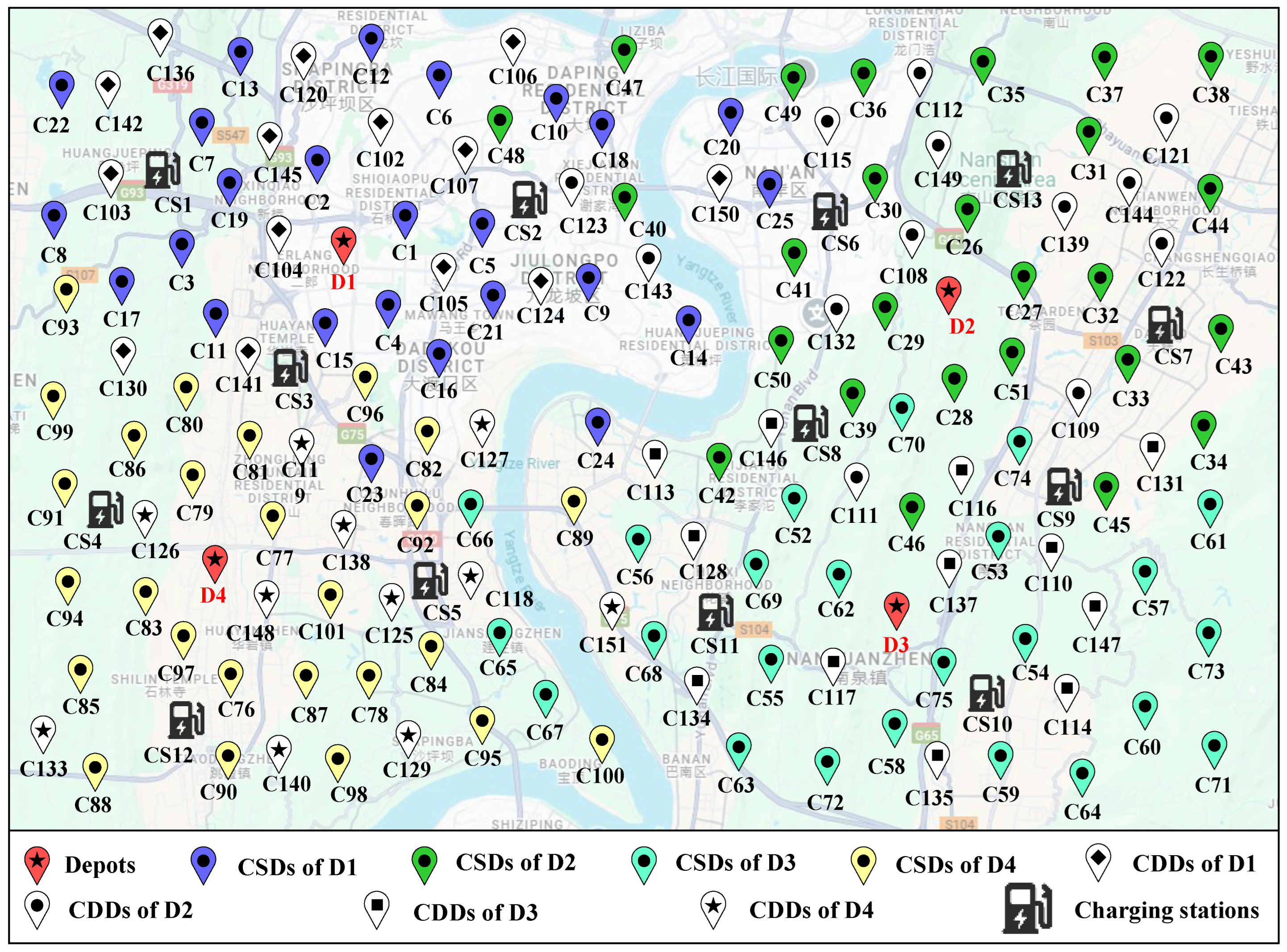
| Depots | CSDs | Charging Stations |
|---|---|---|
| D1 | C1-C25 | CS1, CS2, CS3 |
| D2 | C26-C51 | CS6, CS7, CS8, CS13 |
| D3 | C52-C75 | CS9, CS10, CS11 |
| D4 | C76-C101 | CS4, CS5, CS12 |
| Parameters | Definition | Value |
|---|---|---|
| Arc-specific coefficient of electric vehicle | 0.11 | |
| Arc-specific coefficient of electric truck | 0.13 | |
| Vehicle-specific coefficient of electric vehicle | 0.78 | |
| Vehicle-specific coefficient of electric truck | 0.97 | |
| Weight of electric truck t, (unit: kg) | 1500 | |
| Weight of electric vehicle v, (unit: kg) | 3800 | |
| Windward area of electric vehicle (unit: m2) | 2.41 | |
| Acceleration of electric vehicle (unit: m/s2) | 0 | |
| Gravity constant (unit: m/s2) | 9.81 | |
| Road inclination angle from node i to node j, | 0 | |
| Air density (unit: kg/m3) | 1.2041 | |
| Air drag coefficient | 0.48 | |
| Rolling resistance coefficient | 0.01 | |
| Drive train efficiency of electric vehicle | 0.89 | |
| Price per electricity unit (unit: USD/kW·h) | 2 | |
| Charging rate of electric vehicle v, (unit: kw·h/h) | 30 | |
| Operating cost per charging station (unit: USD) | 70 | |
| Penalty cost per time unit of earliness | 5 | |
| Penalty cost per time unit of delay | 10 | |
| Rental cost of electric truck | 100 | |
| Rental cost of electric vehicle | 150 | |
| I | Insertion cost for each dynamic demand | 25 |
| Load capacity of electric truck t, (unit: kg) | 210 | |
| Load capacity of electric vehicle v, (unit: kg) | 1000 | |
| Battery capacity of electric vehicle (unit: kw·h) | 70 | |
| Fixed cost of depot k, | 200 | |
| max_iteration | Maximum number of iterations | 200 |
| pop_size | Population size | 100 |
| pc | Crossover probability | 0.8 |
| ps | Selection probability | 0.7 |
| pm | Mutation probability | 0.15 |
| Scenario | pc | ps | pm | ||||||
|---|---|---|---|---|---|---|---|---|---|
| Value | ATOC (USD) | SD | Value | ATOC (USD) | SD | Value | ATOC (USD) | SD | |
| 1 | 0.05 | 10,175 | 14 | 0.05 | 10,120 | 13 | 0.01 | 10,205 | 2 |
| 2 | 0.1 | 10,157 | 18 | 0.1 | 10,153 | 19 | 0.02 | 10,158 | 3 |
| 3 | 0.15 | 10,199 | 17 | 0.15 | 10,169 | 14 | 0.04 | 10,132 | 2 |
| 4 | 0.2 | 10,191 | 12 | 0.2 | 10,169 | 9 | 0.06 | 10,144 | 4 |
| 5 | 0.25 | 10,186 | 9 | 0.25 | 10,145 | 7 | 0.08 | 10,124 | 4 |
| 6 | 0.3 | 10,201 | 7 | 0.3 | 10,131 | 6 | 0.1 | 10,139 | 3 |
| 7 | 0.35 | 10,155 | 7 | 0.35 | 10,157 | 6 | 0.15 | 10,120 | 2 |
| 8 | 0.4 | 10,197 | 8 | 0.4 | 10,141 | 7 | 0.2 | 10,131 | 5 |
| 9 | 0.45 | 10,179 | 6 | 0.45 | 10,131 | 6 | 0.25 | 10,136 | 7 |
| 10 | 0.5 | 10,126 | 5 | 0.5 | 10,199 | 4 | 0.3 | 10,130 | 6 |
| 11 | 0.55 | 10,191 | 4 | 0.55 | 10,195 | 5 | 0.35 | 10,143 | 8 |
| 12 | 0.6 | 10,166 | 5 | 0.6 | 10,120 | 8 | 0.4 | 10,218 | 14 |
| 13 | 0.65 | 10,082 | 5 | 0.65 | 10,149 | 5 | 0.45 | 10,206 | 13 |
| 14 | 0.7 | 10,117 | 3 | 0.7 | 10,120 | 3 | 0.5 | 10,174 | 12 |
| 15 | 0.75 | 10,085 | 4 | 0.75 | 10,131 | 5 | 0.55 | 10,288 | 16 |
| 16 | 0.8 | 10,120 | 1 | 0.8 | 10,194 | 4 | 0.6 | 10,196 | 16 |
| 17 | 0.85 | 10,134 | 2 | 0.85 | 10,114 | 4 | 0.65 | 10,254 | 19 |
| 18 | 0.9 | 10,127 | 2 | 0.9 | 10,125 | 3 | 0.7 | 10,218 | 16 |
| 19 | 0.95 | 10,128 | 2 | 0.95 | 10,137 | 4 | 0.75 | 10,275 | 15 |
| 20 | 1 | 10,146 | 16 | 1 | 10,197 | 6 | 0.8 | 10,322 | 21 |
| Customers | C20 | C23 | C24 | C25 | C40 | C42 | C45 | C46 | C47 | C48 | C65 | C66 | C67 | C70 | C74 | C80 | C89 | C93 | C96 |
|---|---|---|---|---|---|---|---|---|---|---|---|---|---|---|---|---|---|---|---|
| Initial depot | D1 | D1 | D1 | D1 | D2 | D2 | D2 | D2 | D2 | D2 | D3 | D3 | D3 | D3 | D3 | D4 | D4 | D4 | D4 |
| Final depot | D2 | D4 | D3 | D2 | D1 | D3 | D3 | D3 | D1 | D1 | D4 | D4 | D4 | D2 | D2 | D1 | D3 | D1 | D1 |
| Case | Depot | FOC (USD) | CTC (USD) | EDC (USD) | PC (USD) | IC (USD) | RC (USD) | TOC (USD) | NCS | NEV | NET |
|---|---|---|---|---|---|---|---|---|---|---|---|
| Initial | D1 | 410 | 0 | 1885 | 248 | 0 | 600 | 3143 | 3 | 6 | 0 |
| D2 | 480 | 0 | 2512 | 273 | 0 | 500 | 3765 | 4 | 5 | 0 | |
| D3 | 410 | 0 | 3047 | 308 | 0 | 600 | 4365 | 3 | 6 | 0 | |
| D4 | 410 | 0 | 2083 | 254 | 0 | 700 | 3447 | 3 | 7 | 0 | |
| Total | 1710 | 0 | 9527 | 1083 | 0 | 2400 | 14,720 | 13 | 24 | 0 | |
| Optimized | D1 | 340 | 187 | 1069 | 84 | 400 | 350 | 2430 | 2 | 2 | 1 |
| D2 | 340 | 166 | 1306 | 82 | 350 | 450 | 2694 | 2 | 3 | 1 | |
| D3 | 410 | 218 | 1422 | 90 | 175 | 350 | 2665 | 3 | 2 | 1 | |
| D4 | 340 | 180 | 1046 | 90 | 325 | 350 | 2331 | 2 | 2 | 1 | |
| Total | 1430 | 751 | 4843 | 346 | 1250 | 1500 | 10,120 | 9 | 9 | 4 |
| Starting Depots | Service Period | Routes | Final Depot | EVs |
|---|---|---|---|---|
| D1 | (1,14) | D1→C7→C13→C136*→C142*→C22→CS1→C103*→C8→C19→D1 | D1 | EV1 |
| (1,14) | D1→C2→C12→C6→C106*→C47→C10→C18→CS2→C48→C107*→C1→D1 | D1 | EV2 | |
| (1,14) | D1→C102*→C120*→C145*→D1 | D1 | EV1 | |
| (15,24) | D1→C4→C16→C21→C124*→C9→C14→C143*→C40→C123*→CS2→C5→C105*→D1 | D1 | EV2 | |
| (15,24) | D1→C15→C96→C81→C119*→C77→D4 | D4 | EV1 | |
| (15,24) | D1→C104*→C3→C17→C93→C130*→C80→C141*→C11→D1 | D1 | EV1 | |
| D2 | (1,14) | D2→C29→C132*→C50→C41→C25→C150*→C20→CS6→C30→C108*→D2 | D2 | EV3 |
| (1,14) | D2→C27→C32→C122*→C44→C121*→C38→C37→C31→CS13→C144*→C139*→D2 | D2 | EV4 | |
| (1,14) | D2→C51→C109*→C33→C43→C34→C131*→CS9→C74→C28→D2 | D2 | EV5 | |
| (15,24) | D2→C26→C149*→C115*→C49→C36→C112*→C35→CS13→D2 | D2 | EV3 | |
| (15,24) | D2→C39→C70→C146*→C111*→D3 | D3 | EV4 | |
| D3 | (1,14) | D3→C137*→C53→C46→C116*→CS9→C45→C61→C57→C110*→D3 | D3 | EV6 |
| (1,14) | D3→C54→C147*→C73→C71→C60→C64→C114*→CS10→C75→D3 | D3 | EV7 | |
| (15,24) | D3→C117*→C58→C59→C135*→C72→C63→C55→D3 | D3 | EV4 | |
| (15,24) | D3→C62→C52→C42→C89→C56→D3 | D3 | EV8 | |
| D4 | (1,14) | D4→C138*→C92→C66→C118*→C151*→CS11→C68→C134*→D3 | D3 | EV8 |
| (1,14) | D4→C97→C85→C133*→C88→CS12→C90→C140*→C98→C87→C76→D4 | D4 | EV9 | |
| (15,24) | D4→C23→C82→C127*→C24→C113*→C128*→CS11→C69→D3 | D3 | EV9 | |
| (15,24) | D4→C79→C86→C99→C91→C94→C83→C126*→D4 | D4 | EV7 | |
| (15,24) | D4→C148*→C78→C129*→C95→C100→C67→C65→CS5→C84→C125*→C101→D4 | D4 | EV6 |
| Case | TOC (USD) | EC (kWh) | EDC (USD) | PC (USD) | IC (USD) | RC (USD) | FOC (USD) | NEV | NET | NCS |
|---|---|---|---|---|---|---|---|---|---|---|
| Case 1 | 14,720 | 4763 | 9527 | 1083 | 0 | 2400 | 1710 | 24 | 0 | 13 |
| Case 2 | 12,769 | 3622 | 7245 | 764 | 1250 | 1800 | 1710 | 18 | 0 | 13 |
| Case 3 | 10,120 | 2421 | 4843 | 346 | 1250 | 1500 | 1430 | 9 | 4 | 9 |
| Mode | FOC (USD) | CTC (USD) | EDC (USD) | PC (USD) | IC (USD) | RC (USD) | TOC (USD) | NEV | NET | NCS |
|---|---|---|---|---|---|---|---|---|---|---|
| Mode 1 | 1710 | 0 | 9527 | 1083 | 0 | 2400 | 14,720 | 24 | 0 | 13 |
| Mode 2 | 1430 | 751 | 6514 | 437 | 1250 | 1800 | 12,182 | 12 | 4 | 9 |
| Mode 3 | 1500 | 751 | 6810 | 461 | 1250 | 2000 | 12,772 | 14 | 4 | 10 |
| Mode 4 | 1430 | 751 | 4843 | 346 | 1250 | 1500 | 10,120 | 9 | 4 | 9 |
Disclaimer/Publisher’s Note: The statements, opinions and data contained in all publications are solely those of the individual author(s) and contributor(s) and not of MDPI and/or the editor(s). MDPI and/or the editor(s) disclaim responsibility for any injury to people or property resulting from any ideas, methods, instructions or products referred to in the content. |
© 2025 by the authors. Licensee MDPI, Basel, Switzerland. This article is an open access article distributed under the terms and conditions of the Creative Commons Attribution (CC BY) license (https://creativecommons.org/licenses/by/4.0/).
Share and Cite
Wang, Y.; Chen, C.; Wei, Y.; Wei, Y.; Wang, H. Collaboration and Resource Sharing for the Multi-Depot Electric Vehicle Routing Problem with Time Windows and Dynamic Customer Demands. Sustainability 2025, 17, 2700. https://doi.org/10.3390/su17062700
Wang Y, Chen C, Wei Y, Wei Y, Wang H. Collaboration and Resource Sharing for the Multi-Depot Electric Vehicle Routing Problem with Time Windows and Dynamic Customer Demands. Sustainability. 2025; 17(6):2700. https://doi.org/10.3390/su17062700
Chicago/Turabian StyleWang, Yong, Can Chen, Yuanhan Wei, Yuanfan Wei, and Haizhong Wang. 2025. "Collaboration and Resource Sharing for the Multi-Depot Electric Vehicle Routing Problem with Time Windows and Dynamic Customer Demands" Sustainability 17, no. 6: 2700. https://doi.org/10.3390/su17062700
APA StyleWang, Y., Chen, C., Wei, Y., Wei, Y., & Wang, H. (2025). Collaboration and Resource Sharing for the Multi-Depot Electric Vehicle Routing Problem with Time Windows and Dynamic Customer Demands. Sustainability, 17(6), 2700. https://doi.org/10.3390/su17062700