Determinants of Design with Multilayer Perceptron Neural Networks: A Comparison with Logistic Regression

Abstract

This research focuses on harnessing artificial neural networks (ANNs) to enhance the design of steel structures. The design process encompasses various stages, including defining the building’s geometry, estimating loads, selecting an appropriate structural system, sizing components, and creating detailed plans. Optimizing the weight of these structures is vital for reducing costs, improving efficiency, and minimizing environmental impact. This study specifically investigates multilayer perceptron (MLP) neural networks to optimize steel structure design. It evaluates different ANN configurations with varying numbers of hidden layers and neurons to find the most effective arrangement. Additionally, the performance of MLP networks is compared to that of logistic regression. The results demonstrate that MLP networks deliver superior accuracy in optimizing the design of steel structures compared to logistic regression. The process of designing steel structures at an early stage can reduce the consumption of energy and raw materials before the production of the structures themselves begins. This is important from an economic point of view because some costs can be reduced during the design process. When designing steel structures, it is also possible to take into account changing conditions, such as the growing share of renewable energy sources in the total energy balance in many countries.

1. Introduction

The application of steel structures in building construction is widespread due to their numerous advantages, including strength, versatility, and ease of construction. Steel structures are commonly used in a wide range of buildings, such as bridges, skyscrapers, stadiums, warehouses, and industrial plants. In particular, skyscrapers often utilize composite steel–concrete structures, primarily to meet the rigorous fire safety requirements but also to provide the necessary bearing capacity for these high-rise, heavy-load buildings. The combination of steel and concrete in such structures offers the ideal balance of fire resistance, structural integrity, and load-bearing efficiency, ensuring both safety and performance in the face of the demanding conditions that skyscrapers must withstand [1]. However, despite the many advantages of steel structures, there are also some inherent disadvantages, especially when compared to concrete structures. One of the main drawbacks of steel is its vulnerability to high temperatures, which can cause a significant loss of strength during a fire. This necessitates additional fireproofing measures such as intumescent coatings or concrete encasement, which can increase both the initial cost of construction and long-term maintenance. Additionally, steel structures are more susceptible to corrosion over time, particularly in harsh environmental conditions, requiring ongoing treatment and protection to prevent deterioration. Concrete, in contrast, offers better inherent fire resistance and is generally more durable, which may reduce the need for extensive fireproofing and maintenance over the lifespan of the structure. Furthermore, concrete has higher compressive strength, making it a more suitable material for certain heavy-load applications, whereas steel is typically used for its strength-to-weight ratio and flexibility.

Steel structures are valued for their high strength-to-weight ratio, enabling efficient material use and resilience against heavy loads and harsh conditions. They also offer design versatility, allowing for diverse architectural forms. The design and construction process involves multiple steps [2]. First, the building geometry is designed, considering factors like function and occupancy. Gravity and lateral loads are then calculated to choose and size the structural system. Detailed drawings are prepared, and quality control is established. Steel components are fabricated in a workshop and transported to the construction site for assembly using cranes, bolts, and welds, adhering to safety protocols [3].

Optimizing the weight of steel structures is vital for cost reduction, improved transportation and fabrication efficiency, and reduced environmental impact. Engineers can achieve this by using efficient design principles and structural systems like trusses or space frames to distribute loads and minimize steel usage [4]. By analyzing structural requirements and using innovative design approaches, excess steel can be eliminated. High-strength steels and finite element analysis (FEA) help reduce steel usage while maintaining structural integrity, considering cost, availability, and fabrication factors [5].

Composite materials like steel–concrete structures reduce steel usage while maintaining strength. Modular construction techniques improve manufacturing precision, minimize waste, and speed up project completion. Value engineering evaluates design alternatives for cost-effective weight optimization. Effective collaboration among architects, engineers, and contractors is crucial [6]. Involving all stakeholders early helps identify weight reduction strategies. Weight optimization must prioritize structural integrity and safety, ensuring compliance with load and code requirements. By applying efficient design principles, selecting materials carefully, using advanced analysis techniques, employing composite materials, modular construction, value engineering, and fostering collaboration, engineers can optimize the weight of steel structures. This leads to cost savings, improved construction efficiency, reduced environmental impact, and enhanced structural performance [7]. Building Information Modeling (BIM) plays a crucial role in enhancing the efficiency and effectiveness of the design and construction process. By providing a digital representation of the physical and functional characteristics of a structure, BIM allows for better coordination between all project stakeholders, including architects, engineers, and contractors. This collaboration facilitates the identification and implementation of weight reduction strategies early in the design phase. BIM also enables real-time data sharing and updates, which helps minimize errors and conflicts, leading to improved construction precision and reduced waste. Additionally, by integrating BIM with advanced optimization techniques, such as the use of composite materials, modular construction, and value engineering, engineers can make more informed decisions that result in cost savings, reduced environmental impact, and enhanced structural performance. The ability to visualize and simulate the entire lifecycle of a project in a virtual environment further aids in meeting safety standards, ensuring compliance with load requirements, and optimizing the weight of steel structures.

To optimize skeletal structures with discrete design variables, Ref. [8] modeled the improved arithmetic optimization algorithm (IAOA), a version of the arithmetic optimization algorithm (AOA). The IAOA addresses the regular AOA’s issues of poor exploration and premature convergence by requiring fewer algorithm-specific parameters and enhancing exploration and exploitation capabilities. Its effectiveness is proven through three benchmark structural optimization problems, showing better performance than standard AOA and other techniques. Ref. [8] discusses the use of ANNs to optimize the design of reinforced concrete columns with H-shaped steel sections, improving accuracy and reducing effort, cost, and CO₂ emissions [9,10,11,12,13].

Ref. [14] simulated a method for optimizing the design of steel frame structures with plate shear walls that combines modified dolphin echolocation (DE) with bat optimization approaches. The goal is to minimize the structure’s weight while meeting design requirements. The algorithm selects optimal beam and column sections from a list by analyzing multiple wall designs per span. Results show that the modified DE algorithm is superior to the bat technique for medium- and high-rise structures, while both methods aid in optimizing low-rise building designs. The Enhanced Crystal Structure Algorithm (ECryStAl), which optimizes gable frameworks with tapering members, was modeled by the authors of [15]. ECryStAl includes enhancements like grade-D crystal selection, dynamic crystal inclusion, and a reduced search range to optimize gable frame design. When compared to four other meta-heuristic methods, ECryStAl consistently achieves more optimal, lighter designs for gable frames with tapered members. To reduce material consumption and guarantee occupant comfort in tall buildings experiencing wind-induced vibrations, Refs. [16,17,18,19,20,21] conducted a bi-objective integrated design framework that makes use of dynamic vibration absorbers (DVAs). The framework optimizes DVA tuning to minimize floor acceleration and structural sizing optimization for minimum-weight design. The outcomes show notable decreases in the amount of steel used and embodied carbon emissions, providing a novel strategy for high-rise structures that use less material [22,23,24,25,26,27].

The two-material truss topology optimization algorithm for lowering a structure’s global warming potential (GWP) is presented by the authors of [28]. The algorithm determines each truss element’s cross-sectional area and material composition, optimizing for various objectives and constraints like GWP minimization and stress constraints. Its effectiveness in reducing embodied carbon in structural design is demonstrated using glue-laminated timber and steel in 2D and 3D truss designs. Ref. [29] explores innovative energy solutions for buildings by integrating waste streams and alternative sources like human power and animal body heat into sustainable architecture. Ref. [30] uses AI algorithms to optimize the mix design for Steel Fibre Reinforced Concrete (SFRC), achieving high accuracy in predicting compressive and flexural strength, and providing optimal mix solutions [31,32,33].

Recent research in steel structure optimization has focused on improving material efficiency, reducing costs, and minimizing environmental impact. Several computational methods and design strategies have been explored to enhance the performance and sustainability of steel structures. Finite Element Analysis (FEA) and Artificial Neural Networks (ANNs) are among the most widely used tools, enabling precise predictions and optimization of structural behavior while reducing material waste. Moreover, optimization algorithms, such as the Arithmetic Optimization Algorithm (AOA) and Genetic Algorithms (GA), have been applied to optimize steel structure designs. These algorithms aim to minimize material usage while ensuring structural integrity and safety. In addition to computational methods, high-strength steels, composite materials, and modular construction techniques are increasingly utilized to achieve lightweight designs and improved efficiency. The use of multi-objective optimization frameworks, which balance multiple performance criteria, has also gained attention. These approaches focus on optimizing not only the weight and cost of steel structures but also their environmental impact. For instance, the integration of dynamic vibration absorbers (DVAs) in high-rise buildings has shown the potential to reduce steel consumption while improving comfort and safety. Furthermore, there has been significant progress in the development of innovative hybrid approaches, such as the Enhanced Crystal Structure Algorithm (ECryStAl) and hybrid algorithms combining dolphin echolocation and bat optimization techniques. These methods have been particularly effective in optimizing complex structural systems like gable frames and plate shear wall structures. Overall, the current state of research highlights the continuous evolution of techniques aimed at achieving more sustainable, cost-effective, and efficient designs in steel structure optimization. However, challenges remain in balancing structural safety, material efficiency, and environmental impact, requiring ongoing collaboration among engineers, architects, and contractors to develop innovative solutions.

The structure of the rest of this paper is as follows: The technique is presented in Section 2, the results are discussed and analyzed in detail in Section 3, and the conclusion section contains the final thoughts.

2. Methodology

Neural networks, in terms of structural analysis and hardware implementation, have been continuously advancing in terms of quantity, quality, and capability. Various techniques of neural computing are still emerging and evolving. The concept of neural networks draws inspiration from the expectations placed on these networks and their similarities to real biological networks [29]. The exploration of neural networks began when scientists recognized the brain as a dynamic system with a parallel and highly parallel processing structure, which is fundamentally different from conventional processors. The structure of the brain consists of a vast network of neurons that communicate with each other through electrical and chemical signals. Neurons are the fundamental building blocks of the nervous system and can be found throughout the brain, spinal cord, and peripheral nervous system [30]. Neurons in the brain vary in size and shape depending on their location and function, contributing to cognitive abilities like perception, memory, and decision-making. Neurons are connected through synapses, allowing signals to transmit and form complex neural activity patterns. Artificial Neural Networks (ANNs) are inspired by the brain’s structure and aim to replicate its information-processing capabilities for tasks like pattern recognition and decision making. ANNs consist of input, output, and hidden layers, with interconnected nodes that enable learning from complex data, making them a key component of machine learning [34].

ANNs use weights to define connection strengths, which are initially set randomly and then adjusted via optimization methods like gradient descent. They require large, diverse datasets for effective training, as biased data can degrade performance, and overfitting can hinder generalization. The training process involves forward propagation (calculating outputs through weighted sums and activation functions) and backward propagation (adjusting weights based on errors). Regularization techniques like early stopping and dropout help avoid overfitting. Due to their complexity, ANNs are hard to interpret, motivating research into methods for improving their explainability [35]. Convolutional Neural Networks (CNNs), specialized for visual data, consist of convolutional, pooling, and fully connected layers. These networks detect patterns at multiple levels, making them effective for tasks like image classification and object detection. Their hierarchical structure allows them to generalize well to unseen data and handle variations in scale, rotation, and translation [36]. Recurrent Neural Networks (RNNs) excel in processing sequential data, capturing temporal dependencies with internal memory. LSTM cells, which help address the vanishing gradient problem, are often used to model long-term dependencies in tasks such as language processing and time-series forecasting [37]. Proper initialization of parameters is critical in multi-layer perceptrons. Random initialization is common, but poor choices can slow convergence or lead to local minima. Correct initialization improves training efficiency and prevents stagnation [38]. One statistical model used for binary classification tasks is logistic regression. This kind of regression analysis uses a categorical dependent variable that reflects two possible outcomes, usually denoted by the numbers 0 and 1. Estimating the likelihood that a dependent variable will fall into a specific category based on one or more independent variables is the aim of logistic regression.

The logistic function, sometimes referred to as the sigmoid function, is used in logistic regression to model the dependent variable. Any real integer can be converted to a value between 0 and 1 using the sigmoid function. This makes it possible for us to interpret the logistic regression’s result as a probability [39]. The logistic function is defined as:

$$f(x)={\displaystyle \frac{1}{1+e^{-x}}}$$

(1)

where x is the linear predictor, which is a function of the independent variables [40]. The linear predictor is usually written as:

$$x={\beta }_0+{\beta }_1{x}_1+{\beta }_2{x}_2+\dots +{\beta }_n{x}_n$$

(2)

where the independent variables are $x_1$, $x_2$, …, $x_n$, the intercept is ${\beta }_0$, and the coefficients are ${\beta }_1$, ${\beta }_2$, …, ${\beta }_n$. Each independent variable’s impact on the dependent variable’s log odds is shown by the coefficients.

The log odds of the dependent variable and the independent variables are assumed to have a linear relationship by the logistic regression model. The natural logarithm of the odds ratio is the log odds, sometimes referred to as the logit. The possibility of the event happening in relation to the likelihood that it will not happen is represented by the odds ratio. The odds ratio can be transformed into a linear connection that can be studied using conventional regression approaches by taking its logarithm. The definition of log odds is:

$$\log ({\displaystyle \frac{p}{1-p}})$$

(3)

where $p$ is the probability of the dependent variable being 1. The log odds are equal to the linear predictor, so we can write [41]:

$$\log ({\displaystyle \frac{p}{1-p}})={\beta }_0+{\beta }_1{x}_1+{\beta }_2{x}_2+\dots +{\beta }_n{x}_n$$

(4)

One popular method for estimating the parameters of the logistic regression model is the maximal likelihood estimation (MLE) technique. The maximum likelihood of observing the provided data is what the MLE approach looks for when determining parameter values. The product of the probabilities of each observation, given the parameter values, is the likelihood function. The likelihood function’s natural logarithm makes up the easier-to-work-with log-likelihood function. For logistic regression, the log-likelihood function is [42,43]:

$$\mathcal{l}(\beta )={\displaystyle {\sum }_{i=1}^N}[y_i\mathrm{l}\mathrm{o}\mathrm{g}({\displaystyle \frac{1}{1+e^{-x_i\beta }}})+(1-y_i)\mathrm{l}\mathrm{o}\mathrm{g}({\displaystyle \frac{e^{-x_i\beta }}{1+e^{-x_i\beta }}})]$$

(5)

where N is the number of observations, y_i is the dependent variable for the ith observation, x_i is the vector of independent variables for the ith observation, and β is the vector of coefficients. Finding the values of β that result in the largest possible log-likelihood function is the first step in the MLE approach. Usually, an iterative optimization approach like gradient descent is used for this. The logistic regression model can be trained and then used to analyze new data to provide predictions. Based on the values of the independent variables, the model determines the likelihood that the dependent variable will fall into the positive class (such as 1). The probabilities can then be translated into binary forecasts by setting a threshold. A statistical metric for evaluating the direction and strength of a linear relationship between two variables is the correlation coefficient (r). The formula below is used to compute it:

$$r={\displaystyle \frac{n(\sum xy)-(\sum x)(\sum y)}{\sqrt{[n\sum x^2-(\sum x{)}^2\left]\right[n\sum y^2-(\sum y{)}^2]}}}$$

(6)

The individual data points from the two variables are represented by $x_i$ and $y_i$ in this formula. Summation is indicated by the $\mathsf{\Sigma }$ sign, which means that every data point should have the formula applied to it.

The covariance between the two variables, which quantifies how they vary jointly, is computed using the formula’s numerator. Normalizing the covariance, the denominator is the product of the standard deviations of the $x$ and $y$ variables.

Following calculation, the correlation coefficient’s value can be understood as follows:

• r = 1: A complete positive correlation exists, indicating a proportionate increase in one variable for every unit increase in the other.
• A perfect negative correlation, or r = −1, means that when one variable rises, the other falls proportionately.
• r = 0: The variables’ association is not linear.

It is crucial to remember that the correlation coefficient may not take non-linear relationships between variables into account and can only represent linear interactions. Furthermore, a high correlation between two variables does not always imply that one variable causes the other to change. This is known as the concept of causation denial.

Mean Absolute Error is referred to as MAE. A regression or forecasting problem is a statistical metric that is used to calculate the average size of errors or deviations between expected and actual values.

The formula for calculating MAE is as follows:

$$MAE=\left({\displaystyle \frac{1}{n}}\right)\mathsf{\Sigma }\left|y_i-{\hat{y}}_i\right|$$

(7)

where:

• $y_i$ represents the actual (true) value.
• ${\hat{y}}_i$ represents the predicted value.
• $\mathsf{\Sigma }$ represents the summation symbol, indicating that the formula should be applied to each data point.
• $n$ represents the total number of data points.

The mean absolute error (MAE) computes the absolute deviation between each expected and actual number, adds up all of the deviations, and finally finds the average. It gives the average absolute difference between the values that were anticipated and those that were observed. When assessing the performance of regression and machine learning models, MAE is frequently employed. Without taking into account the direction of the mistakes, it shows the average magnitude of errors in the anticipated values. Better model performance is indicated by a lower MAE, which denotes fewer variances between actual values and forecasts.

Root Mean Square Error is referred to as RMSE. A regression or forecasting problem is a statistical metric that is used to calculate the average size of errors or deviations between expected and actual values. When greater errors have a more noticeable effect on the evaluation, RMSE is especially helpful. The following formula can be used to calculate RMSE:

$$RMSE=\surd \left(\mathsf{\Sigma }\right(y_{i}i-{\hat{y}}_{i}i)2/n)$$

(8)

where:

• $y_i$ represents the actual (true) value.
• ${\hat{y}}_i$ represents the predicted value.
• $\mathsf{\Sigma }$ represents the summation symbol, indicating that the formula should be applied to each data point.
• $n$ represents the total number of data points.

RMSE computes the square root of the result by first calculating the squared difference between each predicted and actual value, adding up those squared differences, and determining the average. Taking into account both the direction and size of the deviations, the RMSE gives an estimate of the average magnitude of the mistakes. It shows the spread or dispersion of the mistakes and is a representation of the residuals’ standard deviation. Better model performance is shown by a lower RMSE since it denotes smaller discrepancies between actual values and forecasts.

ANN-Based Feature Transformation: Suppose the ANN transforms the input features X into a new set of features Z, where Z = f_ANN(X). The ANN consists of weights W, biases B, and activation functions, with the transformation defined as:

$$\mathit{zj}=\tanh ({\displaystyle \sum _{i=1}^n}\mathit{wij}.\mathit{xi}+\mathit{Bj})\hspace{1em}\hspace{1em}\forall j\in \{1,\dots ,m\}$$

(9)

where tanh is the hyperbolic tangent activation function for the hidden layer, and mm is the number of neurons in the hidden layer.

Finally, it should be noted that in addition to the algorithms considered above, algorithms like whale methods [44], fuzzy-based approaches [45], and other heuristics and conventional algorithms [46] can be utilized in steel structure optimization.

3. Results and Discussions

3.1. Multilayer Perceptron Architecture

A multilayer perceptron (MLP) neural network is employed for the task at hand. The coefficients for the training method are determined through extensive study and are utilized to effectively halt the training process. To enhance the network’s ability to generalize, cross-validation techniques are also applied. The dataset is divided into three categories: training, evaluation, and testing. Various evaluation metrics are used to assess the accuracy and performance of the MLP neural networks. In this study, an MLP with a single hidden layer is primarily utilized. Upon completion of the training, the weight values are stored, making the network ready for deployment. Each MLP model incorporates either one or two hidden layers, with the hyperbolic tangent function serving as the activation function for the hidden layers, while the output layer employs the sigmoid function.

Given that the number of neurons in the hidden layer significantly impacts the network’s behavior, a comprehensive study was conducted to evaluate performance across different neuron configurations. In the initial model, the error metrics of the MLP network with one hidden layer were analyzed across the evaluation, training, and testing datasets. All networks demonstrated reasonably acceptable performance, leading to the selection of networks with 34 and 104 neurons in the hidden layer due to their superior performance. These four networks were further evaluated against the evaluation and testing datasets, each containing 14 samples. Ultimately, the network with 104 neurons in the hidden layer was chosen as the optimal structure for the MLP model. It exhibited the best correlation coefficients in both the evaluation and training datasets, as well as lower MAE and RMSE values in the evaluation and testing datasets. Despite having a higher maximum error in the evaluation dataset compared to the other three networks, its overall performance justifies its selection. The source of the dataset was Kaggle (Kaggle.com accessed on 25 February 2025).

Figure 1 illustrates the relationship between the RMSE values and the number of epochs for the train, test, and validation datasets. The x-axis represents the number of epochs, which denotes the iterations of the learning process applied to the training dataset, while the y-axis displays the RMSE values, indicating the model’s prediction accuracy compared to actual outcomes. A lower RMSE score signifies a better fit for the model.

The blue train line indicates the RMSE for the training dataset. As the number of epochs increases, the RMSE value gradually decreases, suggesting that the model is enhancing its accuracy and reducing prediction errors as it learns from the training data. The red test line represents the RMSE for the test dataset, which also starts at a higher value and decreases with more epochs. The close proximity of the train and test lines implies that the model performs well across both datasets, with minimal discrepancies.

The green validation line illustrates the RMSE for the validation dataset, which is primarily used to fine-tune the model and mitigate overfitting. Although the validation line also decreases with the number of epochs, it remains slightly higher than the train and test lines, indicating that the model’s performance on the validation dataset is somewhat inferior. This could suggest potential overfitting or underfitting issues. Overfitting occurs when the model becomes too tailored to the training data, while underfitting arises when the model is overly simplistic and fails to capture the data’s underlying patterns.

3.2. Impact of Hidden Neuron Count in Validation (Single Hidden Layer)

The number of hidden neurons plays a crucial role in the performance of a neural network during validation. Figure 2 illustrates how different configurations of hidden neurons affect performance, evaluated through three key metrics: R, RMSE, and MAE. The R value indicates the strength and direction of the linear relationship between predicted and observed values, with a range from −1 to 1. Meanwhile, RMSE and MAE assess the average magnitude of prediction errors, where lower values signify a better fit and reduced variation. The analysis reveals that the neural network with 20 hidden neurons achieves optimal performance, characterized by the highest R value, as well as the lowest RMSE and MAE. In contrast, the network with 30 hidden neurons demonstrates the poorest validation results, marked by the lowest R, alongside the highest RMSE and MAE.

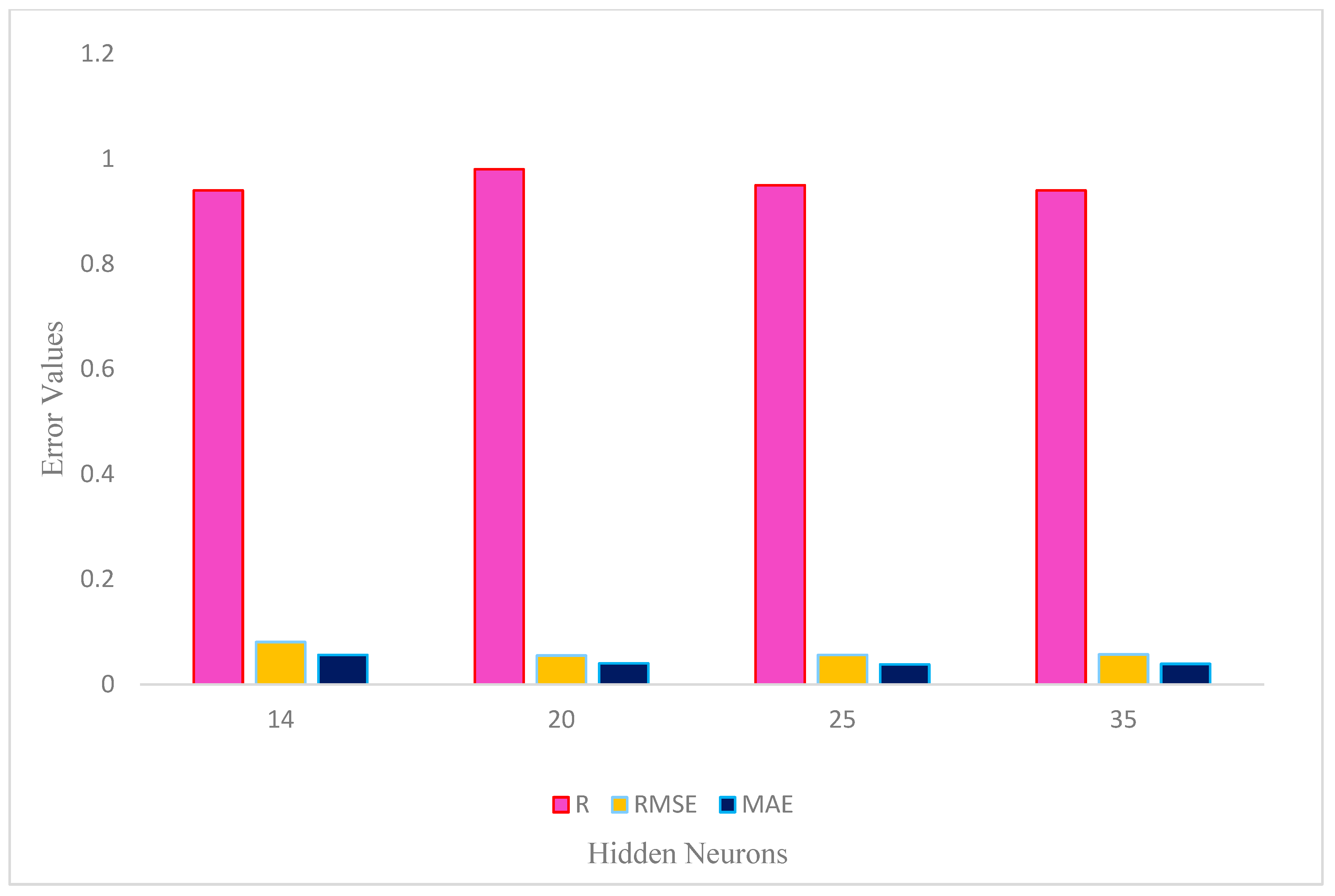
3.3. Impact of Hidden Neuron Count in Training (Single Hidden Layer)

Figure 3 illustrates the performance results of a neural network trained with varying numbers of hidden neurons in a single hidden layer. The evaluation metrics employed are R, RMSE, and MAE. Among the configurations tested, the neural network with 20 hidden neurons delivered the best performance, achieving an impressive R value of 0.98, which indicates a strong linear relationship between the predicted and observed values. Furthermore, it recorded the lowest RMSE of 0.055 and the lowest MAE of 0.04, highlighting its superior accuracy and reduced prediction variation compared to other models. Neural networks with 14, 25, and 35 hidden neurons also performed commendably, with R values of 0.94, 0.95, and 0.94, respectively. These configurations demonstrated similar RMSE and MAE values, reflecting comparable prediction accuracy. Overall, the neural network with 20 hidden neurons stands out for its exceptional training performance, marking it as the most effective configuration among those evaluated.

3.4. Impact of Hidden Neuron Count in Testing (Single Hidden Layer)

For the testing phase, the neural network with 14 hidden neurons achieved an R value of 0.92, indicating a relatively strong linear relationship between the predicted and observed values. It had an RMSE of 0.086 and an MAE of 0.08, suggesting a moderate average magnitude of prediction errors. The neural network with 20 hidden neurons performed slightly better, with an R value of 0.93. It had an RMSE of 0.081 and an MAE of 0.058, indicating improved accuracy and less variation compared to the configuration with 14 hidden neurons. Similarly, the neural networks with 25 and 35 hidden neurons exhibited R values of 0.91 and 0.88, respectively (Figure 4). They had similar RMSE and MAE values, indicating comparable performance in terms of prediction accuracy.

3.5. Influence of Hidden Neuron Count in Validation (Two Hidden Layers)

Figure 5 presents the validation results of a neural network with different configurations of hidden layers. The neural network with 30 neurons in both layers achieved the highest performance, exhibiting a strong linear relationship (R = 0.99) and the lowest RMSE and MAE values. The configurations with 25 neurons in both layers also performed well, while the configurations with 14 neurons or a combination of 14 and 20 neurons showed lower performance with weaker linear relationships and higher prediction errors. Overall, the neural network with 30 neurons in both layers demonstrated the best performance during the validation phase.

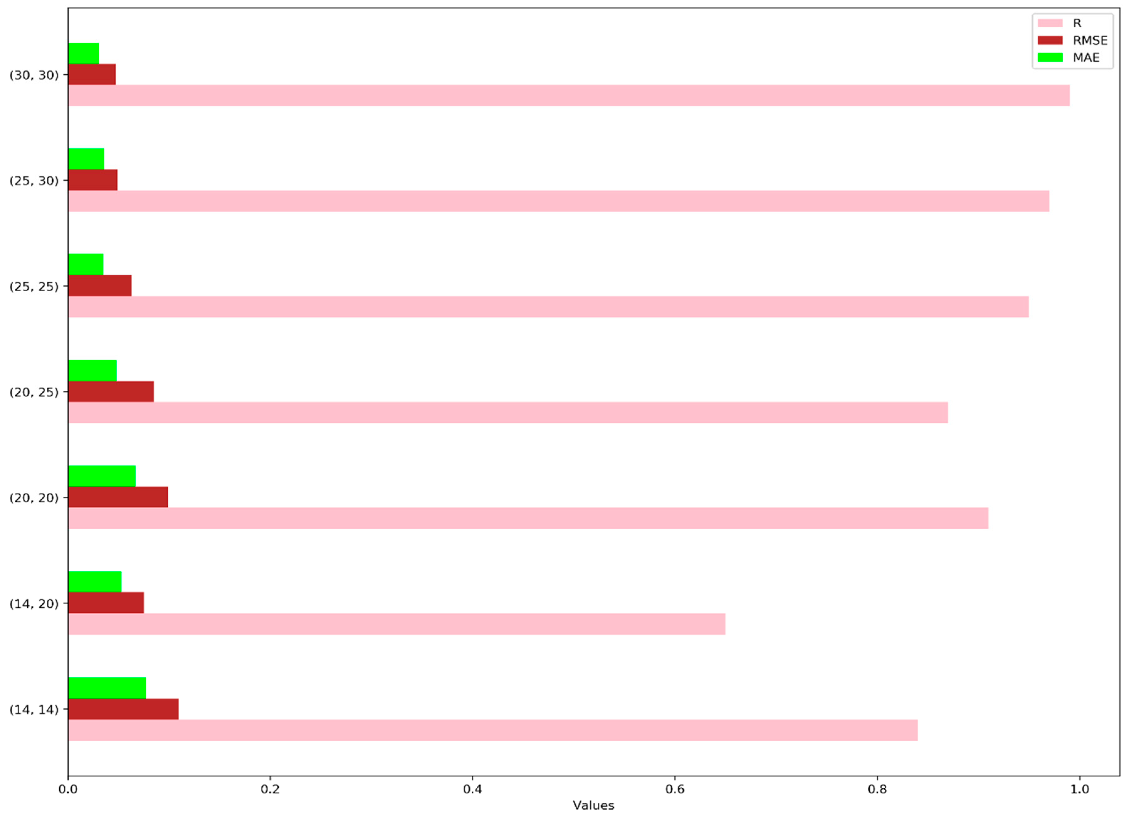
Figure 6 presents different configurations of hidden layers in a neural network along with their corresponding evaluation metrics. These configurations are specifically used for training the model. The evaluation metrics include the R, RMSE, and MAE. Upon analyzing the results, it becomes evident that increasing the number of hidden neurons in both layers leads to improvements in the evaluation metrics. As we progress from the first row to the last row, the R increases from 0.8 to 0.95. This increase indicates a stronger linear relationship between the predicted and actual values during the training process. Furthermore, as the number of hidden neurons increases, both the RMSE and MAE values decrease. These decreasing values suggest that the model’s predictions align more closely with the actual training data, indicating improved accuracy. These observations underscore the significance of the neural network’s architecture, particularly the number of hidden neurons, in shaping the model’s performance during the training phase. By incorporating a larger number of hidden neurons, the model becomes more adept at capturing intricate patterns within the training data, thereby enhancing its predictive accuracy.

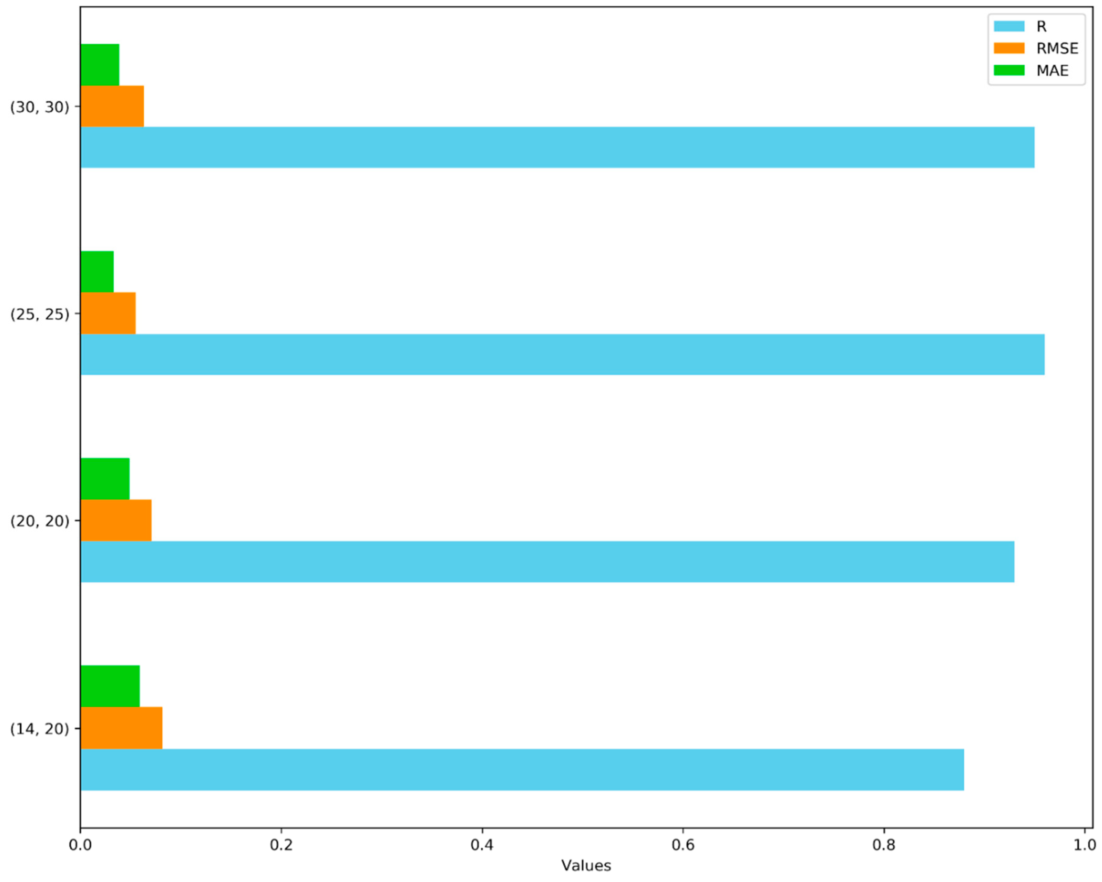
3.6. Influence of Hidden Neuron Count in Testing (Two Hidden Layers)

Figure 7 that the highest values for all three metrics occur when the neural network has hidden layers with 30 neurons each. This configuration results in a highly accurate prediction model for the observed data. Conversely, the lowest values for all three metrics are observed when the neural network has hidden layers with 14 and 20 neurons. This suggests that the prediction model is less accurate for observations within this range. The intermediate values for the metrics are seen when the neural network has hidden layers with 20 and 25 neurons or 25 and 30 neurons. These ranges indicate that the prediction model has moderate accuracy for observations within these ranges.

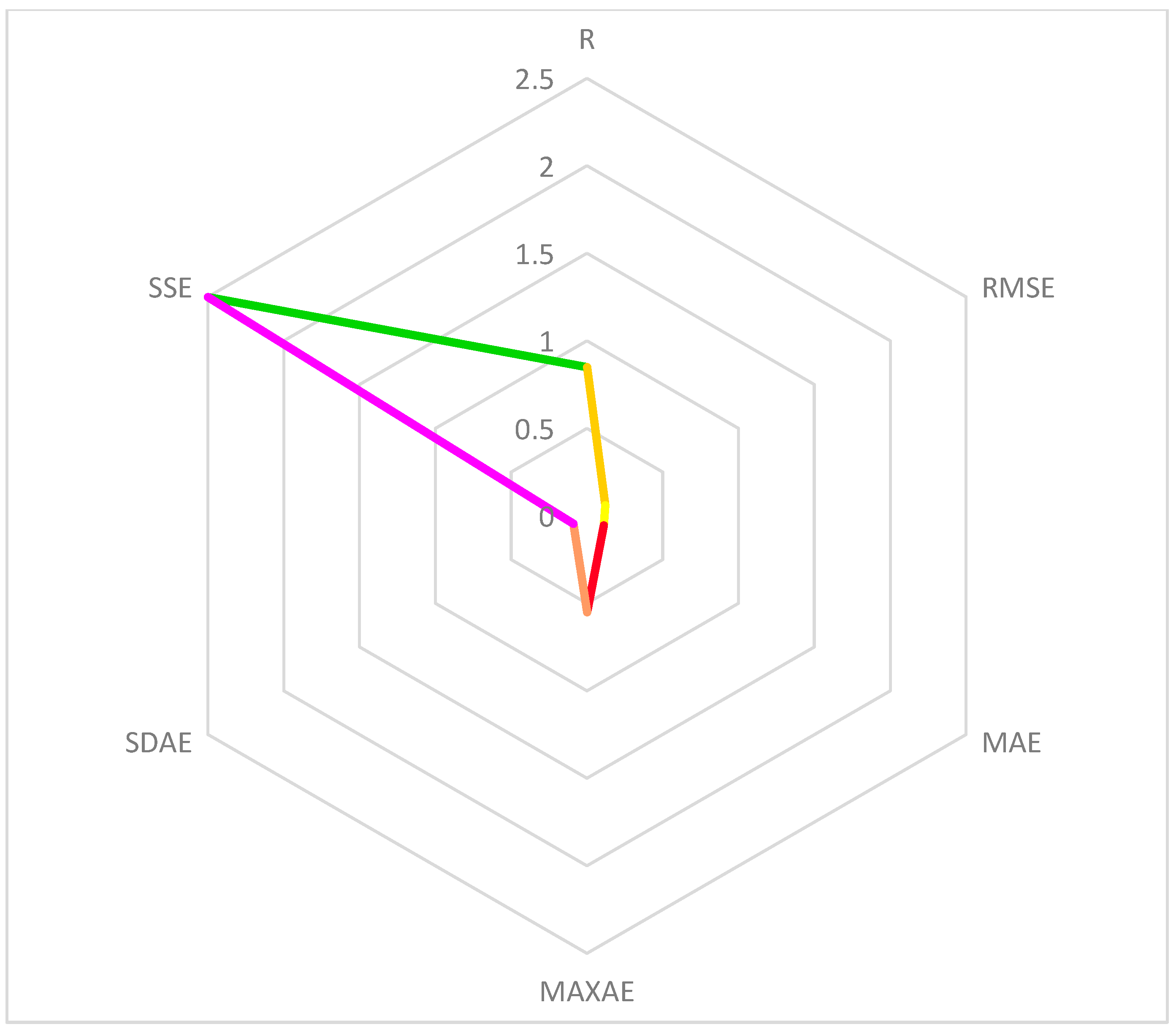
3.7. Logistic Regression Method Performance

In the logistic regression method, the following results were obtained. The logistic regression model accounts for 85% of the variance in the dependent variable, according to the coefficient of determination (R-squared), which is 0.85. The average magnitude of the prediction errors is indicated by the RMSE value of 0.12. A lower RMSE suggests that the model is performing better. The average absolute difference between the expected and actual values is represented by the MAE value, which is 0.11. A lower MAE indicates that the model is more accurate. Out of all the forecasts, the MAXAE value of 0.55 shows the highest absolute error. The greatest difference between the expected and actual values is shown by this. The average standard deviation of the prediction errors is indicated by the SDAE number, which is 0.09. Less error variability is indicated by a lower SDAE. The sum of the squared deviations between the actual and anticipated values is represented by the SSE value, which is 2.5. A model that fits the data better overall has a lower SSE. These findings offer an assessment of the logistic regression model’s efficacy and precision in forecasting the binary outcomes. The effectiveness of the logistic regression approach is demonstrated in Figure 8.

3.8. Logistic Regression Performance in Comparison with MLP

The Multilayer Perceptron method demonstrated better accuracy and performance compared to the logistic regression method. The MLP model showed superior performance in terms of predictive accuracy and capability to capture complex relationships in the data. This is evidenced by its higher coefficient of determination and lower error metrics such as RMSE, MAE, MAXAE, SDAE, and SSE. The MLP’s ability to model non-linear relationships and its flexibility in capturing intricate patterns in the data contribute to its improved performance compared to logistic regression, which assumes a linear relationship between the predictors and the outcome variable.

The results from our study clearly indicate that the Multilayer Perceptron (MLP) neural network outperforms logistic regression in the context of optimizing the design of steel structures. Specifically, Figure 9 illustrates that the accuracy of the MLP method is approximately 2 percent higher than that of logistic regression when predicting binary outcomes. This superior performance can be attributed to the inherent capabilities of MLPs. Unlike logistic regression, which is a linear model, MLPs are capable of capturing complex, non-linear relationships in the data due to their multiple layers and activation functions. This allows MLPs to better model the intricate dependencies and interactions that may exist in the design parameters of steel structures, leading to more accurate predictions. Therefore, the evidence provided in Figure 9, along with the theoretical understanding of the models, supports the claim that MLP achieves higher accuracy compared to logistic regression for this particular application.

Factors such as building geometry and loads play an essential role in influencing the design and optimization of steel structures. The geometry of the building determines the overall shape and layout, which in turn impacts how loads are distributed and transferred throughout the structure. Different shapes and configurations can lead to variations in stress and strain, which affects the performance, stability, and safety of the structure. For example, intricate or irregular shapes might cause stress concentrations, leading to potential weak points, whereas more straightforward designs might allow for better load distribution and overall stability.

In addition to geometry, the types and magnitudes of loads acting on the structure are critical. Gravity loads include the weight of the building itself, its contents, and occupants. These loads are constant and must be accurately calculated to ensure the structure can support its weight. Lateral loads, such as those from wind, earthquakes, and snow, can vary significantly based on location, climate, and usage. These loads can introduce dynamic forces that require the structure to have flexibility and resilience to prevent damage or failure. Wind loads can exert pressure that may cause swaying or bending, while seismic loads from earthquakes can create complex vibrational forces that necessitate robust joint connections and ductility in the structural components. Accurate estimation and consideration of these loads are essential to ensure that the structure can withstand various forces without compromising its integrity. This involves detailed load calculations, simulations, and the use of safety factors to account for uncertainties and variabilities. By focusing on these factors, engineers can optimize the design for cost efficiency, safety, and environmental impact. Effective load management ensures the use of materials is both efficient and sustainable, reducing excess weight and the associated costs.

Moreover, incorporating these considerations early in the design process can lead to innovative solutions such as the use of high-strength materials, modular construction techniques, and advanced analysis tools like finite element analysis (FEA). These strategies not only enhance the structure’s performance but also improve its adaptability to changing conditions, such as the increasing integration of renewable energy sources and evolving building codes. Ultimately, by carefully analyzing and addressing the influences of building geometry and loads, engineers can design steel structures that are not only structurally sound but also cost-effective, energy-efficient, and environmentally friendly, leading to more effective and resilient steel structures that meet modern standards and expectations.

4. Conclusions

This study explored the application of ANNs, specifically MLP models, in optimizing the design of steel structures. Steel structures are widely used in the construction industry due to their high strength-to-weight ratio, adaptability, and durability under various loading and environmental conditions. The design and construction process involves several critical steps, including defining structural geometry, evaluating loads, selecting an appropriate structural system, sizing components, and generating detailed construction plans. The findings of this research highlight the effectiveness of ANN-based models in improving the design process by enhancing environmental sustainability, increasing productivity, and achieving cost savings. The study compared different ANN configurations and found that optimizing the number of hidden layers and neurons significantly influences the accuracy of the predictive model. MLP models demonstrated superior performance compared to logistic regression, achieving higher predictive accuracy and lower error metrics (R = 0.93, RMSE = 0.081, MAE = 0.058 for 20 neurons in the hidden layer). The results indicate that MLP networks can efficiently capture complex, non-linear relationships in structural design optimization, leading to more precise and efficient designs. By leveraging ANN-based techniques, material consumption can be minimized, reducing waste and promoting sustainable construction practices that lower the carbon footprint of building projects. Additionally, the use of ANN models streamlines the design process by providing optimal solutions more quickly, thereby reducing the time and resources required for iterative design modifications. The cost-effectiveness of optimized designs further contributes to efficient resource utilization, ultimately lowering overall project expenses. While this study demonstrates the potential of ANN-based optimization in steel structure design, several areas warrant further exploration to enhance the applicability and effectiveness of these models:

• Advanced Machine Learning Techniques: Future research could incorporate more sophisticated deep learning models, such as CNNs and RNNs, to improve predictive accuracy. Hybrid models integrating ANNs with evolutionary algorithms, reinforcement learning, or genetic algorithms could provide more robust optimization solutions.
• Real-World Validation and Case Studies: While the current study focuses on computational modeling, future work could involve real-world case studies to validate the effectiveness of ANN-based optimization in practical construction projects. Implementing these models in live engineering applications and comparing their performance with traditional design methods will further strengthen their credibility.
• Multi-Objective Optimization: The optimization framework could be expanded to consider multiple objectives beyond weight reduction, such as structural resilience, lifecycle cost analysis, and sustainability metrics. Multi-objective evolutionary algorithms (MOEAs) combined with ANN models could provide more balanced design solutions.
• Adaptation to Dynamic and Uncertain Conditions: The construction industry is subject to changing material costs, evolving design standards, and environmental uncertainties. Future research should explore probabilistic modeling and uncertainty quantification techniques to enhance the robustness of ANN-based design recommendations.
• Integration with BIM: A key advancement would be the integration of ANN-based optimization models with BIM, enabling an automated, data-driven approach to structural design. This integration would facilitate collaboration among engineers, architects, and project managers, streamlining the design process and improving project efficiency.
• Automated Design Recommendations and Expert Systems: Further research could explore the development of AI-driven expert systems that provide automated design recommendations for steel structures based on real-time data inputs. These systems could assist engineers in making informed decisions while adhering to industry standards and regulations.