Demand Response Strategies for Electric Vehicle Charging and Discharging Behavior Based on Road–Electric Grid Interaction and User Psychology

Abstract

With the rapid increase in electric vehicle (EV) ownership, the uncertainty of EV charging demand has become a significant concern, especially in distributed photovoltaic (PV) power distribution networks (DNs) with high penetration rates. This growing demand presents challenges in meeting the needs of EV owners and grid charging/discharging stations (GCDSs), jeopardizing the stability, efficiency, reliability, and sustainability of the DNs. To address these challenges, this study introduces innovative models, the anchoring effect, and regret theory for EV demand response (DR) decision-making, focusing on dual-sided demand management for GCDSs and EVs. The proposed model leverages the light spectrum optimizer–convolutional neural network to predict PV output and utilizes Monte Carlo simulation to estimate EV charging load, ensuring precise PV output prediction and effective EV distribution. To optimize DR decisions for EVs, this study employs time-of-use guidance optimization through a logistic–sine hybrid chaotic–hippopotamus optimizer (LSC-HO). By integrating the anchoring effect and regret theory model with LSC-HO, this approach enhances satisfaction levels for GCDSs by balancing DR, enhancing voltage quality within the DNs. Simulations on a modified IEEE-33 system confirm the efficacy of the proposed approach, validating the efficiency of the optimal scheduling methods and enhancing the stable operation, efficiency, reliability, and sustainability of the DNs.

1. Introduction

1.1. Background

With the escalation of environmental and resource challenges, there is a worldwide agreement on the necessity to reshape the energy framework and encourage the adoption of renewable energy sources. The efficient and sustainable use of energy is crucial and recognized as a key strategy to address current energy issues [1,2,3]. In this context, photovoltaic (PV) systems and electric vehicles (EVs) are being more commonly employed in distribution networks (DNs) as efficient solutions [4,5]. The integration of large-scale EVs and PV systems into DNs introduces complexities to the existing energy structure, operational procedures, and dispatch strategies of DNs. Consequently, the optimization of EV scheduling and PV forecasting within DNs has emerged as a key research focus [6] and aims to enhance the efficiency, reliability, and sustainability of DNs. Previous study efforts seek to advance the transition towards a greener and more resilient energy system, fostering greater integration of renewable energy sources and promoting sustainable energy practices on a global scale.

1.2. Related Literature

The output of a photovoltaic system is inherently characterized by high levels of stochasticity and volatility. The accurate prediction of PV power plays a crucial role in ensuring the safe and cost-effective operation of high-penetration renewable power systems. This predictive technology forms the cornerstone for effectively integrating PV generation into the grid and optimizing the scheduling of EV charging and discharging behavior. Machine learning algorithms have attracted considerable attention in the prediction of PV output, prompting researchers to compare different algorithms to determine the most appropriate predictive model for PV systems [7]. Kumar Ganti P proposed a method that combines the sparrow search algorithm and gradient-boosting decision tree to enhance the efficiency of PV output prediction [8]. Wu S. combined the complementary ensemble empirical mode decomposition with the adaptive noise decomposition method with a hybrid neural network for PV output prediction [9]. Abou Houran M. proposed a composite model that integrates long short-term memory (LSTM) and swarm intelligence optimization algorithms to improve the accuracy of short-term offshore PV output prediction [10]. Ren X. proposed the quad kernel–convolutional neural network (CNN) model and applied it to PV output prediction [11]. Wang L. proposed a prediction method based on ensemble empirical mode decomposition to improve LSTM models for PV output prediction [12]. This study creatively applies the light spectrum optimizer (LSO) to optimize CNN hyperparameters, thereby improving the accuracy, resilience, and efficiency of PV prediction.

With the increasing number of EVs, the planning and management of charging infrastructure have become crucial. To achieve efficient load forecasting, Mahmoudi E. proposed a model merging the travel trajectories of the EV’s daily trips to forecast spatial–temporal urban charging power demand [13]. Yin W. proposed an integrated prediction model that enhances the accuracy of EV charging through short-term load forecasting [14]. Liu K. proposed a stochastic EV equilibrium-based method for forecasting EV charging loads [15]. Shen H. proposed a hybrid deterministic–stochastic method for forecasting EV charging loads [16]. Lu J. proposed a real-time interactive multi-source information-based system for forecasting EV charging loads, integrating deep learning frameworks, and speed–flow models [17]. Therefore, this study thoroughly examines the EV load forecasting methods proposed in the mentioned research and utilizes the concept of trip chains to depict the spatial–temporal paths of EVs. By taking into account the shortest paths and spatial locations of both DNs and the road network, this study forecasts the spatial–temporal charging loads of EVs, demonstrating the spatial–temporal linkage among DNs, the road network, and EVs.

Research has concentrated on developing innovative approaches for EV charging coordination and scheduling to optimize the spatial–temporal distribution of EV charging loads. Lin R. proposed a linear quadratic mean field game theory with a major player to optimize the scheduling management of parking lots and formulate decentralized charging control strategies for multiple EVs [18]. Zhao Z. investigated the EV charging scheduling issue for public charging stations by employing a two-level hierarchical charging scheduling method [19]. Zhou K. and Liu L. proposed coordinated charging scheduling methods for EVs in microgrids to shift load demand from peak to valley periods [20,21]. The scheduling considered in these studies can effectively decrease EV charging costs. Aghajan-Eshkevari S. provided a comprehensive and updated review of the control structures of EVs in charging stations, objectives of EV management in power systems, and optimization methodologies for charge and discharge management of EVs in energy systems [22]. Wu H. proposed a dynamic personalized charging navigation model based on an improved Dijkstra algorithm [23]. Phipps K. emphasized the importance of efficient smart charging applications in meeting EV mobility needs and risk preferences [24]. Wu F. and Zhang K. introduced methods for analyzing the uncertain adjustability of charging stations under multi-attribute group decision-making of EVs [25,26]. Some of these studies only considered the scheduling of individual grid charging/discharging stations (GCDSs), and some did not take into account the spatial–temporal coupling of EVs. Therefore, in this study, EV scheduling not only considers the spatial–temporal coupling of EVs but also incorporates coordination among all grid charging/discharging stations (GCDSs). Taking the subjective decision-making preferences of EVs as the primary factor, an EV decision-making model is developed to decide on participation in the scheduling process, with the goal of maximizing EV owners’ satisfaction.

Uncoordinated charging of large-scale EVs can strain the grid due to limited charging facilities and inadequate power supply at GCDSs. Efficient scheduling of EV charging is crucial for optimizing operations, reducing costs, and ensuring DNs stability. Liu J., Qureshi U., and Wu J. proposed optimal charging scheduling methods based on response to time-of-use (TOU) [27,28,29]. Obeid H., Qureshi U., and Kandpal B. also proposed methods using TOU to incentivize user behavior at charging stations toward actions that achieve the station operator’s objectives [30,31,32]; the TOU considered in these studies can effectively improve charging schedule. Feng J. proposed a coordinated charging and discharging strategy that integrates EVs and energy storage systems to maintain a balance between supply and demand [33]. Sifakis N.K. proposed an innovative operation scheduling and control virtual prosumer method for spatially distributed large-scale prosumers of Plug-in EVs and renewable energy sources [34]. Jiao F. also proposed a power coordination model to obtain the schedule plans of the main grid; the charging station allocation model is designed to determine the charging power for EVs [35]. These studies treat EVs as virtual energy storage for scheduling, and the results demonstrate the effectiveness of this strategy. Therefore, in this paper, a method is proposed that utilizes TOU to incentivize EVs to participate in demand response, establish an EV charging margin model, and efficiently schedule the EVs that respond to the demand.

1.3. Novelty

This study introduces the PV prediction model based on the LSO-CNN algorithm and the EV charging load prediction model based on Monte Carlo to acquire PV output and EV charging load. To improve the effectiveness of demand response and enhance EV owners’ satisfaction with participation, this study presents an anchoring effect charging-demand demand response (CDDR) decision-making model and a regret theory non-charging-demand demand response (NDDR) decision-making model based on subjective and objective factors of charging demand EVs (CDEVs) and non-charging demand EVs (NDEVs). To improve the voltage quality of GCDSs and increase revenue, the EVs charging margin model and voltage floating threshold band were proposed. Finally, a logistic-sine hybrid chaotic–hippopotamus optimizer (LSC-HO) with TOU is utilized to determine the charging strategies for CDEVs and NDEVs, aiming at achieving optimal overall satisfaction for EVs and GCDSs. This study improves the sustainable utilization of EV flexibility resources, promoting wider adoption of EVs, while simultaneously reducing environmental impact, enhancing EV owners’ satisfaction, and enhancing the efficiency, reliability, and sustainability of DNs.

The main contributions are as follows:

• Propose a novel CNN prediction model based on the LSO to improve PV prediction accuracy;
• Construct an EV spatial–temporal model driving model in the road network, and propose Monte Carlo to simulate the charging load distribution of EVs, to efficiently predict EV distribution;
• Propose an anchoring effect and regret theory decision model to consider the charging scheduling of CDEVs and NDEVs with the influence of subjective and objective factors to tackle the stochastic nature of EV charging loads and enhance EV owners’ satisfaction;
• Propose the EV charging margin model and voltage floating threshold band to improve the voltage quality of charging stations and increase revenue to effectively address errors, effectively enhancing the efficiency, reliability, and sustainability of DNs.
• Propose LSC-HO to guide EVs for charging and discharging behaviors by TOU and obtain the scheduled spatial–temporal charging and discharging loads of CDEVs and NDEVs to improve the sustainable utilization and scheduling efficiency of EVs and flexibility resources.

1.4. Organization

This study is organized as follows: Section 2 utilizes the LSO-CNN for PV prediction. Section 3 applies Monte Carlo simulation for spatial–temporal load prediction of EVs. Section 4 proposes anchoring effect and regret theory decision-making models. Section 5 presents the EVs charging margin model and voltage floating threshold band. Section 6 presents the LSO for the optimal scheduling of EVs-GCDSs. Section 7 performs simulations and analyzes the results. Finally, Section 8 shows the conclusion.

2. PV Output Prediction Method

In this study, we seek to advance the transition towards a greener energy system, fostering a greater integration of renewable energy sources. Therefore, we conduct PV output prediction to better utilize solar energy. Advances in CNN research have improved the precision of neural networks in PV output prediction [36,37]. The LSO is distinguished by its adaptive fine-tuning of search space resolution and velocity, allowing for the rapid and accurate identification of optimal solutions, making it a powerful optimization tool [38,39]. This study introduces an innovative prediction methodology that utilizes CNN for short-term PV forecasting, incorporating historical data as input. Additionally, the LSO optimization is employed to screen and optimize the hyperparameters of CNN, ensuring enhanced prediction accuracy.

2.1. CNN

The CNN is a type of neural network specifically designed to handle data with a known grid-like topology. For example, time series data can be viewed as a one-dimensional grid sampled at regular time intervals, while image data can be seen as a two-dimensional grid composed of pixels. In computation, the network primarily utilizes a mathematical operation known as convolution. This study used the same basic CNN architecture as in our previous research [40].

2.2. LSO

The LSO inspiration is the light dispersions with different angles while passing through rain droplets, causing the meteorological phenomenon of the colorful rainbow spectrum. After the initialization, the normal vector of inner refraction $\overrightarrow{x_{\mathit{nA}}}$, inner reflection $\overrightarrow{x_{\mathit{nB}}}$, and outer refraction $\overrightarrow{x_{\mathit{nC}}}$ are calculated as follows:

$$\overrightarrow{x_{\mathit{nA}}}={\displaystyle \frac{\overrightarrow{x_{t_1}^r}}{\mathit{norm}(\overrightarrow{x_{t_1}^r})}}$$

(1)

$$\overrightarrow{x_{\mathit{nB}}}={\displaystyle \frac{\overrightarrow{x_{t_1}^p}}{\mathit{norm}(\overrightarrow{x_{t_1}})}}$$

(2)

$$\overrightarrow{x_{\mathit{nC}}}={\displaystyle \frac{\overrightarrow{x^{*}}}{\mathit{norm}(\overrightarrow{x^{*}})}}$$

(3)

$$\mathit{norm}\left(\overrightarrow{x}\right)=\sqrt{\sum _{j=0}^{d_1}{x}_m^2}$$

(4)

where $\overrightarrow{x_{t_1}^r}$ is a randomly selected solution from the current population at iteration $t_1$, $\overrightarrow{x_t^p}$ is the current solution at iteration $t_1$, $\overrightarrow{x^{*}}$ is the global best solution ever founded, and $\mathit{norm}\left(\overrightarrow{x}\right)$ indicates the normalized value of a vector. $d_1$ stands for the number of dimensions in an optimization problem. $\overrightarrow{x}$ is the input vector to the norm function to normalize it. $x_m$ is the $m$-th dimension in the input vector $\overrightarrow{x}$.

Then, the vectors of inner and outer refracted and reflected light rays are calculated as follows:

$$\overrightarrow{x_{L1} }={\displaystyle \frac{1}{k^r}}[\overrightarrow{x_{L0}}-\overrightarrow{x_{\mathit{nA}}}(\overrightarrow{x_{\mathit{nA}}}\overrightarrow{x_{L0}})]-x_{\mathit{nA}}{\left|1 - {\displaystyle \frac{1}{{(k^r)}^2}}+{\displaystyle \frac{1}{(k^r{)}^2}}(\overrightarrow{x_{\mathit{nA}}}\overrightarrow{x_{L0}}{)}^2\right|}^{{\displaystyle \frac{1}{2}}}$$

(5)

$$\overrightarrow{x_{L2}}=\overrightarrow{x_{L1}}-2\overrightarrow{x_{\mathit{nB}}}(\overrightarrow{x_{L1}}\overrightarrow{x_{\mathit{nB}}})$$

(6)

$$\overrightarrow{x_{L3}}=k^r[\overrightarrow{x_{L2}}-\overrightarrow{x_{\mathit{nC}}}(\overrightarrow{x_{\mathit{nC}}}\overrightarrow{x_{L2}})]+\overrightarrow{x_{\mathit{nC}}}{\left|1-(k^r{)}^2+(k^r{)}^2(\overrightarrow{x_{\mathit{nC}}}\overrightarrow{x_{L2}}{)}^2\right|}^{{\displaystyle \frac{1}{2}}}$$

(7)

where $\overrightarrow{x_{L1}}$, $\overrightarrow{x_{L2}}$, and $\overrightarrow{x_{L3}}$ are the inner refracted, inner reflected, and outer refracted light rays, respectively. $k^r$ stands for the refractive index. $\overrightarrow{x_{L0}}$ is the incident light ray.

After the calculation of the rays’ directions, calculate the candidate solutions according to the value of a randomly generated probability between 0 and 1, $p$ and $q$, then the new candidate solution will be calculated as follows:

$$\overrightarrow{x_{t_1+1} }=\left\{\begin{array}{c}\overrightarrow{x_{t_1} }+ϵR{V}_1^{n}GI(\overrightarrow{x_{L1}}-\overrightarrow{x_{L3}})(\overrightarrow{x_{n1}}-\overrightarrow{x_{n2}}),p\le q\\ \overrightarrow{x_{t_1}}+ϵR{V}_2^{n}GI(\overrightarrow{x_{L2}}-\overrightarrow{x_{L3}})(\overrightarrow{x_{n3}}-\overrightarrow{x_{n4}}),p>q\end{array}\right.$$

(8)

where $\overrightarrow{x_{t_1+1}}$ is the newly generated candidate solution, and $\overrightarrow{x_{t_1}}$ is the current candidate solution at iteration $t_1$. $n1$, $n2$, $n3$, and $n4$ are indices of four solutions selected randomly from the current population. $R{V}_1^n$ and $R{V}_2^n$ are vectors of uniform random numbers that are generated between [0, 1]. $ϵ$ is a scaling factor, and GI is an adaptive control factor based on the inverse incomplete gamma function.

2.3. LSO-CNN

This study leverages LSO-optimized hyperparameters, specifically the initial learning rate and mini-batch size of the CNN, to greatly enhance the efficiency of the CNN. Normalization is applied to handle the variability in data distribution and variable sizes across CNN layers, preventing detrimental learning performance due to discrepancies in weight coefficients.

The flowchart of the LSO-CNN is depicted in Figure 1. PV prediction is conducted using the LSO-CNN through the following steps.

Step 1:

Input the historical data;

Step 2:

Establish the basic structure of the CNN;

Step 3:

Set the parameters of the LSO algorithm;

Step 4:

Initialize the location of the refracted light rays;

Step 5:

Calculate the vectors of the inner and outer refracted and reflected light rays;

Step 6:

Take hyperparameters into the CNN, prediction PV output to obtain the loss, accuracy;

Step 7:

Repeat Steps 4–6 and update the calculation of the rays’ directions in Equation (8) until the current iteration reaches the maximum iteration;

Step 8:

Output the optimal prediction.

3. EV Load Prediction Method

To support the reduction in air pollution and promote sustainable transportation efforts related to EVs, as well as to understand the charging behavior of EVs and the sustainable utilization of EVs’ flexibility resources, in this study, we utilize trip chains and Monte Carlo simulation to model the charging behavior of EVs for more effective sustainable utilization.

3.1. Trip Chain

The trip chain describes the process in which residents depart from home, go through a series of activities, and ultimately return home. This process includes a wealth of information such as spatial, temporal, activity types, and modes of transportation. The trip chain consists of two parts: mobile trajectory points and stationary trajectory points. Mobile trajectory points represent the movement of travelers in space, while stationary trajectory points represent the activities of travelers at a specific location [41,42]. In this study, EV trips are divided into morning trips and evening trips, this paper defines the study zones as residential, working, and recreational zones. It is assumed that the residential zone serves as the starting node for day trips, with the destination being either the working zone or the recreational zone. The probability density of initial departure time, parking time, initial departure node, destination node, and initial SOC are the same as in our previous study [40].

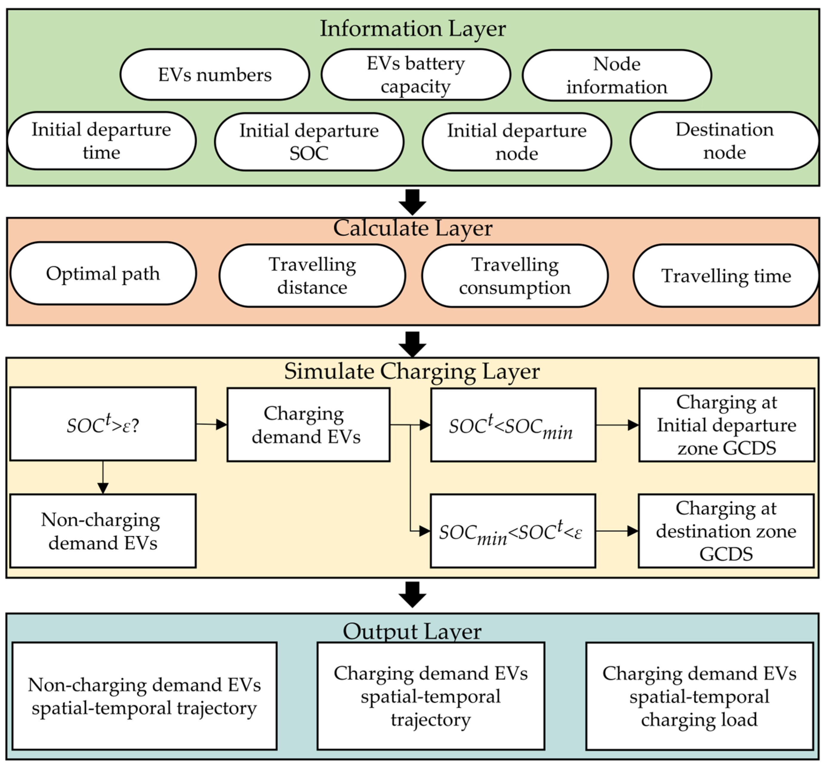
3.2. Monte Carlo Flowchart

The Monte Carlo flowchart is shown in Figure 2.

Step 1:

Input the number of EVs, EV battery capacity, and the node information;

Step 2:

Simulate a single EV’s initial departure time, initial departure SOC, initial departure node, and destination node;

Step 3:

Calculate a single EV’s optimal path, traveling distance, traveling time, and traveling consumption;

Step 4:

Judge whether the EV is charged. If so, update spatial–temporal trajectories; if not, continue the trip until completion;

Step 5:

Update the initial trip chain of each EV;

Step 6:

Repeat Steps 2–5 for the next EV until all EVs are simulated;

Step 7:

Output the NDEV and CDEV spatial–temporal trajectories and CDEV spatial–temporal charging load.

4. EV Demand Response Decision Models and Functions

To improve the sustainable utilization of EVs’ flexibility resources and enhance EV owners’ satisfaction, this study classifies EVs into CDEVs and NDEVs and devises specific demand response decision models and scheduling strategies for CDDR and NDDR. These customized approaches are designed to enhance EV owners’ satisfaction with their charging needs.

4.1. Charging Demand EV Decision Models and Function

4.1.1. Anchoring Effect Decision Model

The anchoring effect, also referred to as the anchoring bias, describes the tendency for individuals in uncertain situations to rely heavily on an initial value, leading to a deviation from the true or objective assessment [43,44,45]. In this study, when EVs engage in CDDR, factors such as TOU, range anxiety, and parking duration act as anchors influencing their decision-making process. Different anchor values have varied impacts on EV owners’ satisfaction to participate in demand response (DR). The anchoring effect utilizes the concepts of a high anchor and low anchor to measure EV owners’ satisfaction towards DR. A high anchor indicates that EVs satisfy a greater impact from DR decisions compared to not participating, while a low anchor suggests lower satisfaction from DR decisions. These anchor values influence EV owners’ satisfaction to participate in DR, with a high anchor typically resulting in higher satisfaction compared to a low anchor.

This study considers EV charging cost, parking overtime charge, and mileage anxiety as EV owners’ satisfaction anchor in DR, then the EV owners’ satisfaction anchor will be calculated as follows:

$${\mathit{Anchor}}_{\mathrm{cc}}={\displaystyle \frac{{\int }_t^{t+T_{\mathit{ch}}^n}{\mathit{Ep}}_{\mathit{ch},\mathit{or}}^t{\eta }_{\mathit{ch}}{P}_{\mathit{ch}}^{t,n}\Delta t}{{\int }_t^{t+T_{\mathit{ch}}^n}{\mathit{Ep}}_{\mathit{ch},\mathit{DR}}^t{\eta }_{\mathit{ch}}{P}_{\mathit{ch}}^{t,n}\Delta t}}$$

(9)

$${\mathit{Anchor}}_{\mathit{poc}}={\displaystyle \frac{P_{\mathit{poc}}\Delta \left(t_{\mathit{dep}}^n-T_{\mathit{ch}}^n\right)}{P_{\mathit{poc},\mathit{DR}}\Delta \left(t_{\mathit{dep}}^n-T_{\mathit{ch}}^n\right)}}$$

(10)

$${\mathit{Anchor}}_{\mathit{ma}}={\displaystyle \frac{e^{\left(a\left(E^i\right)\left(1-\frac{{\mathit{SOC}}_{\mathit{or}}}{{\mathit{SOC}}_{\mathit{chain}}}\right)\right)}+\beta }{e^{\left(a\left(E^i\right)\left(1-\frac{{\mathit{SOC}}_{\mathit{DR}}}{{\mathit{SOC}}_{\mathit{chain}}}\right)\right)}+\beta }}$$

(11)

where ${\mathit{Anchor}}_{\mathit{cc}}$, ${\mathit{Anchor}}_{\mathit{poc}}$, and ${\mathit{Anchor}}_{\mathit{ma}}$ are the satisfaction anchor of charging cost, parking overtime charge, and mileage anxiety, respectively. ${\mathit{Ep}}_{\mathit{ch},\mathit{or}}^t$ and ${\mathit{Ep}}_{\mathit{ch},\mathit{DR}}^t$ are the origin and DR charging price. $T_{\mathit{ch}}^n$ is the total charging time of EVs $n$, ${\eta }_{\mathit{ch}}$ is the charging efficiency, and $P_{\mathit{ch}}^{t,n}$ is the charging power of EVs $n$ at time $t$. $P_{\mathit{poc}}$ and $P_{\mathit{poc},\mathit{DR}}$ are the origin and DR parking overtime price, and $t_{\mathit{dep}}^n$ is the departure time of EVs $n$. a and $\beta$ are the coefficients of mileage anxiety, $E^i$ is the energy consumption of the EV, and ${\mathit{SOC}}_{\mathit{chain}}$ is the SOC of traveling consumption. ${\mathit{SOC}}_{\mathit{or}}$ and ${\mathit{SOC}}_{\mathit{DR}}$ are the origin and DR SOC.

4.1.2. CDEVs Objective Function

The overall decision satisfaction function of the anchoring effect is as follows:

$$a\left({\mathit{SOC}}^t,T_{\mathit{ch}}^n,{\mathit{Ep}}_{\mathit{ch}}^t\right)={\omega }_{\mathit{AE}}{\mathit{Anchor}}_{\mathit{cc}}+{\delta }_{\mathit{AE}}{\mathit{Anchor}}_{\mathit{poc}}+{\gamma }_{\mathit{AE}}{\mathit{Anchor}}_{\mathit{ma}}$$

(12)

where ${\omega }_{\mathit{AE}}$, ${\delta }_{\mathit{AE}}$, and ${\gamma }_{\mathit{AE}}$ are the weight of anchor of charging cost, parking overtime charge, and mileage anxiety, respectively. ${\mathit{SOC}}^t$ is the SOC at time $t$.

And the subject is as follows:

$$\mathrm{A}\left({\mathit{SOC}}^t,T_{\mathit{ch}}^n,{\mathit{Ep}}_{\mathit{ch}}^t\right)<\mathsf{\chi }$$

(13)

where $\mathsf{\chi }$ is the maximum decision satisfaction function of the anchoring effect.

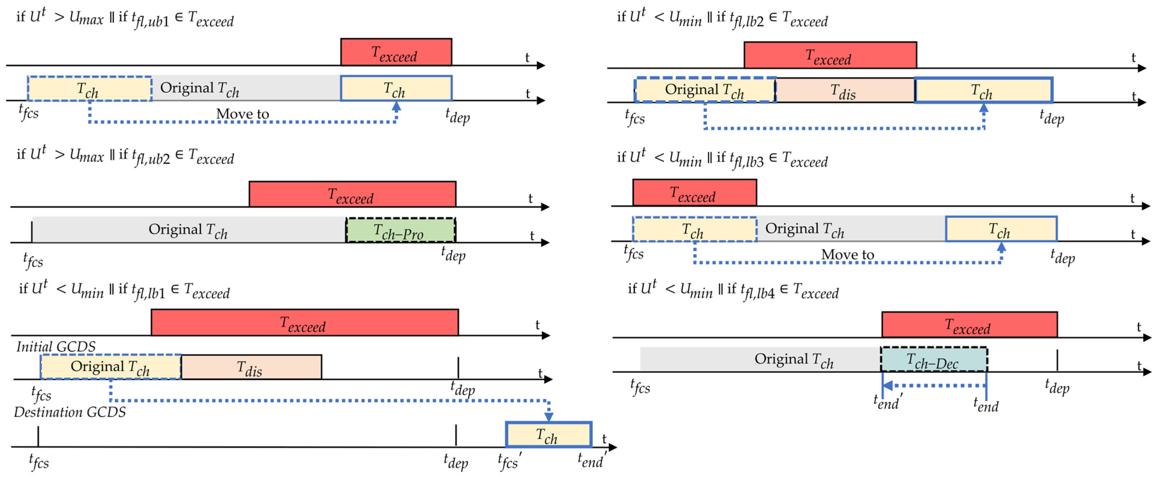
The CDDR flowchart is shown in Algorithm A1 in Appendix A and Figure 3. In this study, six scheduling methods were implemented. If the voltage exceeds the upper limit, consideration is given to transferring the charging time of CDEVs that meet the satisfaction criteria and other conditions within constraints or extending it appropriately. If the voltage falls below the lower limit, consideration is given to transferring the charging time and location, time adjustment, or appropriate shortening of CDEVs that meet the satisfaction criteria and other conditions within constraints. The sequence of judgment for these satisfaction criteria and other conditions within constraints is sequential, with the next scheduling method being assessed only if the previous one fails to meet the criteria. For specific implementation details, please refer to Algorithm A1.

4.2. Non-Charging Demand EVs Decision Models and Function

4.2.1. Regret Theory Decision Model

Regret theory pertains to the psychological state of regret that individuals commonly encounter during the decision-making process [46,47,48]. In this study, when EVs are involved in NDDR, factors such as the ease of engaging in DR, the benefits of charging or discharging, and concerns about mileage anxiety influence their decision-making process. Various levels of regret values have diverse effects on EV owners’ satisfaction in participating in DR. Regret theory evaluates EV owners’ satisfaction in engaging in DR based on high and low regret values. Specifically, a high regret value indicates that EVs experience greater regret for participating in DR decisions than for abstaining, while a low regret value suggests that EVs feel less regret for participating in DR decisions than for not participating. Throughout the process of making DR decisions, different levels of regret values impact EV owners’ satisfaction in engaging in DR in varying ways. Higher regret values typically lead to reduced satisfaction in participating in DR compared to lower regret values.

In this study, EVs’ convenience of DR, charging or discharging benefits, and mileage anxiety are considered as regret values in DR. The regret value for EVs in this context will be calculated as follows:

$$F_{\mathit{conv}}={\omega }_1{\displaystyle \frac{W_{\mathit{fcs}}}{V^{K,t}}}+{\omega }_2{W}_{\mathit{fcs}}{E}^i$$

(14)

$$F_{\mathit{ben}}=\left\{\begin{array}{c}{\omega }_3{\int }_t^{t+T_{\mathit{ch}}^n}{\mathit{Ep}}_{\mathit{ch},\mathit{DR}}^t{\eta }_{\mathit{ch}}{P}_{\mathit{ch}}^{t,n}\Delta t\\ {\omega }_4({\int }_t^{t+T_{\mathit{dis}}^n}{E}_{\mathit{loss}}(\Delta {\mathit{SOC}}_{\mathit{dis}})-{\mathit{Ep}}_{\mathit{ch},\mathit{DR}}^t{P}_{\mathit{dis}}^{t,n}{\displaystyle \frac{\Delta t}{{\eta }_{\mathit{dis}}}})\end{array}\right.$$

(15)

$$F_{\mathit{ma}}={\displaystyle \frac{1}{1+e^{a_1\left(1-\frac{{\mathit{SOC}}^t}{{\mathit{SOC}}_{\mathit{chain}}}\right)+{\beta }_1}}}$$

(16)

where $F_{\mathit{cov}}$, $F_{\mathit{ben}}$, and $F_{\mathit{ma}}$ are the regret value of the convenience of DR, charging or discharging benefits, and mileage anxiety, respectively. ${\omega }_1$, ${\omega }_2$, ${\omega }_3$, and ${\omega }_4$ are the coefficients of the EVs’ convenience of DR and charging or discharging benefits. $W_{\mathit{fcs}}$ is the distance to DR, $V^{K,t}$ is the driving speed of EVs, ${\eta }_{\mathit{dis}}$ is the discharging efficiency, and $P_{\mathit{dis}}^{t,n}$ is the discharging power of EVs $n$ at time $t$. $E_{\mathit{loss}}(·)$ is the calculation of battery charge–discharge loss, $\Delta {\mathit{SOC}}_{\mathit{dis}}$ is discharging SOC of EVs. $a_1$ and ${\beta }_1$ are the coefficients of mileage anxiety.

4.2.2. NDEVs Objective Function

The overall decision satisfaction function of the regret theory is as follows:

$$R\left({\mathit{SOC}}^t,T_{\mathit{ch}}^n,{\mathit{Ep}}_{\mathit{ch}}^t\right)=\ln \left(1+e^{{\xi }_{\mathit{cov}}\left(F_{\mathit{cov}}\right)}\right)+\ln \left(1+e^{{\xi }_{\mathit{ben}}\left(F_{\mathit{ben}}\right)}\right)+\ln \left(1+e^{{\xi }_{\mathit{ma}}\left(F_{\mathit{ma}}\right)}\right)$$

(17)

where ${\xi }_{\mathit{cov}}$, ${\xi }_{\mathit{ben}}$, and ${\xi }_{\mathit{ma}}$ are the weight of the regret value of the convenience of DR, charging or discharging benefits, and mileage anxiety, respectively.

And the subject is as follows:

$$R\left({\mathit{SOC}}^t,T_{\mathit{ch}}^n,{\mathit{Ep}}_{\mathit{ch}}^t\right)<\mathsf{\psi }$$

(18)

where $\mathsf{\psi }$ is the maximum decision satisfaction function of the regret value.

The NDDR flowchart is shown in Algorithm A2. In this study, two scheduling methods were established. If the voltage exceeds the upper limit, consideration is given to the charging behavior of NDEVs that meet the satisfaction criteria and other conditions within constraints. If the voltage falls below the lower limit, consideration is given to the discharging behavior of NDEVs that meet the satisfaction criteria and other conditions within constraints. For specific implementation details, please refer to Algorithm A2.

5. GCDS Scheduling Models and Function

The aim is to improve the sustainable utilization of EVs’ flexibility resources and enhance the efficiency, reliability, and sustainability of DNs. Considering that some EVs have charging periods shorter than their parking time at charging stations, there is a potential for enhancing the initial charging time optimization for EVs within the CDDR framework. Consequently, refining the initial charging times for individual EVs in relation to GCDSs can enhance voltage fluctuation rates, voltage exceeding rates, and GCDS revenue. Therefore, we have developed an EV charging margin model based on EV arrival and departure times at a GCDS. Additionally, we have established a voltage floating threshold band for optimal global EVs DR to escape errors.

5.1. EV Charging Margin Model

This study established an EV charging margin model, which is determined according to the arrival and departure times of EVs at the GCDS. The model is as follows:

$$t_{\mathit{ch}}^n\in \left\{\begin{array}{c}\left(\max \left\{t_{\mathit{arr}}^n,t_{\mathit{exceedub},\mathit{start}}\right\},\min \left\{t_{\mathit{exceedub},\mathit{end}},t_{\mathit{dep}}^n\right\}\right), \mathrm{if} U^t>U_{\mathit{max}}\\ \left(t_{\mathit{arr}}^n,t_{\mathit{exceedlb},\mathit{start}}\right)\mathrm{or}\left(t_{\mathit{exceedlb},\mathit{end}},t_{\mathit{dep}}^n\right), \mathrm{if} U^t<U_{\mathit{min}}\end{array}\right.$$

(19)

where $t_{\mathit{ch}}^n$, $t_{\mathit{arr}}^n$, and $t_{\mathit{dep}}^n$ are the initial charging time, arrival time, and departure time of EVs $n$, respectively. $t_{\mathit{exceedub},\mathit{start}}$, $t_{\mathit{exceedub},\mathit{end}}$, $t_{\mathit{exceedlb},\mathit{start}}$, and $t_{\mathit{exceedlb},\mathit{end}}$ are the starting and ending times of voltage exceeding the upper limit, as well as the starting and ending times of voltage falling below the lower limit, respectively.

5.2. Voltage Floating Threshold Band

Due to guidance, EVs have time lag and response latency, there are also prediction errors in the forecasts. In this study, a voltage threshold band is proposed to predict the voltage at the time $F_t+1$ to advance the CDDR and NDDR scheduling. The main advantages of establishing the voltage threshold band include enhancing the accuracy of predicting voltage changes and optimizing the scheduling arrangements for GCDSs and departures, thereby improving grid stability and charging efficiency. FTB (floating threshold band) utilizes real-time voltage fluctuations to predict the width of FTB of the following interval as follows:

$$U_{\mathit{FTB},\mathit{ub}}^{F_t+1}=U_{\mathit{FTB},\mathit{ub}}-{\Delta U}^{F_t+1}$$

(20)

$$U_{\mathit{FTB},\mathit{lb}}^{F_t+1}=U_{\mathit{FTB},\mathit{lb}}+{\Delta U}^{F_t+1}$$

(21)

where $U_{\mathit{FTB},\mathit{ub}}$ and $U_{\mathit{FTB},\mathit{lb}}$ are the original upper and lower limits, respectively. ${\Delta U}^{F_t+1}$ is the floating margin of FTB at time $F_t+1$.

The floating margin ${\Delta U}^{F_t+1}$ is predicted by sampling spots $t_s$, $t_s\in \left[0,1,2\dots \left(F_t-t+1\right)\right]$, between $t$ and $F_t$ as follows.

$${\Delta U}^{F_t+1}=\max \left\{\left|U^{F_t-t_s}-U^{F_t-t_s-1}\right|\right\}$$

(22)

5.3. GCDS Objective Function

In order to ensure the voltage quality and revenue of the GCDS, utilize voltage fluctuation rates, voltage exceeding rates, and DR costs as the objective functions for GCDS scheduling. The GCDS objective satisfaction functions are as follows:

$$\min \{f_{\mathit{GCDS}}={\theta }_{\mathit{Fr}}\mathit{Fr}+{\theta }_{\mathit{Or}}\mathit{Or}+{\theta }_{\mathit{Re}}\mathit{Re}\}$$

(23)

where $\mathit{Fr}$, $\mathit{Or}$, and $\mathit{Re}$ are the voltage fluctuation rates, voltage exceeding rates, and the revenue of GCDS, respectively. ${\theta }_{\mathit{Fr}}$, ${\theta }_{\mathit{Or}}$, and ${\theta }_{\mathit{Re}}$ are the coefficients of the voltage fluctuation rates, voltage exceeding rates, and the revenue of the GCDS, respectively.

The voltage fluctuation rate is a crucial indicator for assessing voltage stability, as it reflects the magnitude of voltage changes over a period of time. The voltage fluctuation rate functions are as follows:

$$\mathit{Fr}={\displaystyle \frac{\sum _{t=1}^T\frac{\left|U^t-\stackrel{-}{U}\right|}{\stackrel{-}{U}}}{T}}$$

(24)

$$\stackrel{-}{U}={\displaystyle \frac{\sum _{t=1}^T{U}^t}{T}}$$

(25)

where $\stackrel{-}{U}$ is the average value of $U^t$, and $T$ is the total sampling times. $t$ is the sampling spot.

The voltage exceeding rate is also a significant indicator for evaluating voltage stability, as it reflects the number of times the voltage exceeds limits over a period of time. The voltage exceeding rates functions are as follows:

$$\mathit{Or}={\displaystyle \frac{\sum _{t=1}^T{N}_u^t}{T}}$$

(26)

$$N_u^t=\left\{\begin{array}{c}1,U^t<U_{\mathit{min}}\\ 1,U^t>U_{\mathit{max}}\\ 0,U_{\mathit{min}} {<U}^t<U_{\mathit{max}}\end{array}\right.$$

(27)

where $N_u^t$ is to judge whether the node voltage exceeds the limit at time $t$.

The DR costs of GCDS functions are as follows:

$$\mathit{Re}={\int }_{t=1}^T\left({\mathit{Ep}}_{\mathit{ch},\mathit{DR}}^t\right)P_{\mathit{dis}}^t\Delta t/{\eta }_{\mathit{dis}}-\left({\mathit{Ep}}_{\mathit{ch},\mathit{DR}}^t-{\mathit{Ep}}_{\mathit{ch},\mathrm{gc}}^t\right){\eta }_{\mathit{ch}}{P}_{\mathit{ch},\mathit{DR}}^t\Delta t$$

(28)

where ${\mathit{Ep}}_{\mathit{ch},\mathrm{gc}}^t$ is the GCDS cost of electricity procurement.

6. Optimization Algorithms

In this study, tariff and EVs’ initial charging time are utilized as covariates to guide the charging behavior of EVs and optimize the bilateral objective functions of GCDSs and EVs by LSC-HO. HO with fewer parameters, a simple structure, high efficiency, and being easy to understand, is capable of dealing with the multi-peak problem and is superior to the other intelligent algorithms with its faster convergence speed and stronger exploitability.

6.1. HO

The HO is conceived by drawing inspiration from the inherent behaviors observed in hippopotamuses, showcasing an innovative approach in metaheuristic methodology [49,50,51]. The HO is conceptually defined using a trinary-phase model that incorporates their position updating in rivers or ponds, defensive strategies against predators, and evasion methods, which are mathematically formulated.

The initialization process of the HO algorithm involves random initialization, where the initial solutions are randomly generated. The equation for this is as follows:

$$H^{\mathrm{i},\mathrm{j}}=H_{\mathit{min}}^{\mathrm{j}}+r_1(H_{\mathit{max}}^{\mathrm{j}}-H_{\mathit{min}}^{\mathrm{j}})$$

(29)

where $H^{i,j}$ represents the position of the ith candidate solution, $r_1$ is a random number in the range of 0 to 1, and $H_{\mathit{min}}^{\mathrm{j}}$ and $H_{\mathit{max}}^{\mathrm{j}}$ denote the lower and upper bounds of the jth decision variable, respectively.

In the optimization process of this study, exploration is divided into two stages. Exploration Stage 1: updating the hippos positions in the river or pond: Hippos tend to gather closely together, and the dominant hippos are determined iteratively based on the objective function values. The position formula for the male hippos in the group is

$$H_M^{i,j}=H^{i,j}+r_2(D_{\mathit{hippo}}-I_1{H}^{i,j})$$

(30)

where $H_M^{i,j}$ is represents male hippopotamus position, $D_{\mathit{hippo}}$ denotes the dominant hippopotamus position (the hippopotamus that has the best cost in the current iteration), $r_2$ is a random number in the range of 0 to 1, and $I_1$ is an integer between 1 and 2.

When a juvenile hippo has moved away from its mother, the position update formula for both male and female hippos, or for juvenile hippos within the group, is:

$$H_{\mathit{FM}}^{i,j}=\left\{\begin{array}{c}{H}^{i,j}+r_5(D_{\mathit{hippo}}-I_2{\mathit{MG}}^i),T_1>0.6\\ H^{i,j}, \mathrm{else}\end{array}\right.$$

(31)

where $H_{\mathit{FM}}^{i,j}$ is represents female or juvenile hippopotamus position, $r_5$ is a random number in the range of 0 to 1, ${\mathit{MG}}^i$ represents the average value of a randomly selected subset of hippopotamuses, $T_1$ denotes the selection probability, and $I_2$ is an integer between 1 and 2.

Exploration Stage 2: hippo defense against predators: When hippos are attacked by predators or other creatures encroach on their territory, they will trigger a defensive response, using their terrifying jaws to produce sounds that intimidate and repel the attackers. The location where predators or other creatures encroach upon the hippo’s territory is

$$H^{i,j,2}=\left\{\begin{array}{c}\overrightarrow{\mathit{RL}}⨁{\mathit{Predator}}_j+({\displaystyle \frac{b}{c-\mathit{dcos}(2\pi g)}})({\displaystyle \frac{1}{D}}),F_{{\mathit{Predator}}_j}<F_i\\ \overrightarrow{\mathit{RL}}⨁{\mathit{Predator}}_j+({\displaystyle \frac{b}{c-\mathit{dcos}(2\pi g)}})({\displaystyle \frac{1}{2D+r_9}}),F_{{\mathit{Predator}}_j}\ge F_i\end{array}\right.$$

(32)

where $H^{i,j,2}$ is the location where predators or other creatures encroach upon the hippo’s territory, $\overrightarrow{\mathit{RL}}$ is a random vector with a Lévy distribution used to describe the sudden change in the predator’s position when attacking the hippo, ${\mathit{Predator}}_j$ is the position of the predator in the search space, $\mathrm{D}=\left|{\mathit{Predator}}_j-H^{i,j}\right|$ is the distance from the i-th hippo to the predator, $b$, $c$, $d,$ and $g$ are all uniformly distributed random numbers but with different value ranges: $b$ ranges from [2, 4], $c$ ranges from [1, 1.5], $d$ ranges from [2, 3], and $g$ ranges from [2, 4], $r_9$ is a random number in the range of −1 to 1, $F_{{\mathit{Predator}}_j}$ is the factor influencing the hippo’s defensive behavior to protect itself from predator attacks, and $F_i$ is the objective function value.

Development Stage 3: hippos escaping predators: When warnings are ineffective, solitary, sick, and juvenile hippos are particularly vulnerable to predator attacks. Hippos seek to move away from the predator’s area and search for the nearest safe location. The safe position they search for is

$$H^{i,j,3}=H_{\mathit{min}}^{\mathrm{j}}+r_{10}\left[{\displaystyle \frac{H_{\mathit{min}}^{\mathrm{j}}}{t_H}}+r_{11}({\displaystyle \frac{H_{\mathit{max}}^{\mathrm{j}}}{t_H}}-{\displaystyle \frac{H_{\mathit{min}}^{\mathrm{j}}}{t_H}})\right]$$

(33)

where $H^{i,j,3}$ is the hippo’s position as it searches for the nearest safe location, $r_{10}$ is a random number in the range of 0 to 1, $r_{11}$ is a random number that follows a normal distribution, and $t_H$ is the current iteration number.

6.2. LSC-HO

Although the HO algorithm outperforms other algorithms in terms of performance, its random initialization results in significant fluctuations during the optimization process. Moreover, if these issues are not addressed in the hippo position update phase, it can easily lead to unstable optimization results with large deviations and a tendency to get stuck in local optima. To address this, this paper introduces Based on LSC [52,53] in the initialization phase of the HO algorithm to ensure a more uniform distribution of the initial population.

In this paper, a hybrid chaotic mapping that combines the logistic map and the sine map is introduced in the stage of generating the initial population. Replace Equation (29) with Equation (34), the mathematical descriptions of the LSC map is

$$H^{i+1,j}=\mu H^{i,j}(1-{\mathrm{H}}^{\mathrm{i},\mathrm{j}})+(4-\mu )\sin (\pi H^{i,j})/4$$

(34)

where $H^{i+1,j}$ is the solution of the population particle, and $\mu$ is the chaotic multiplier.

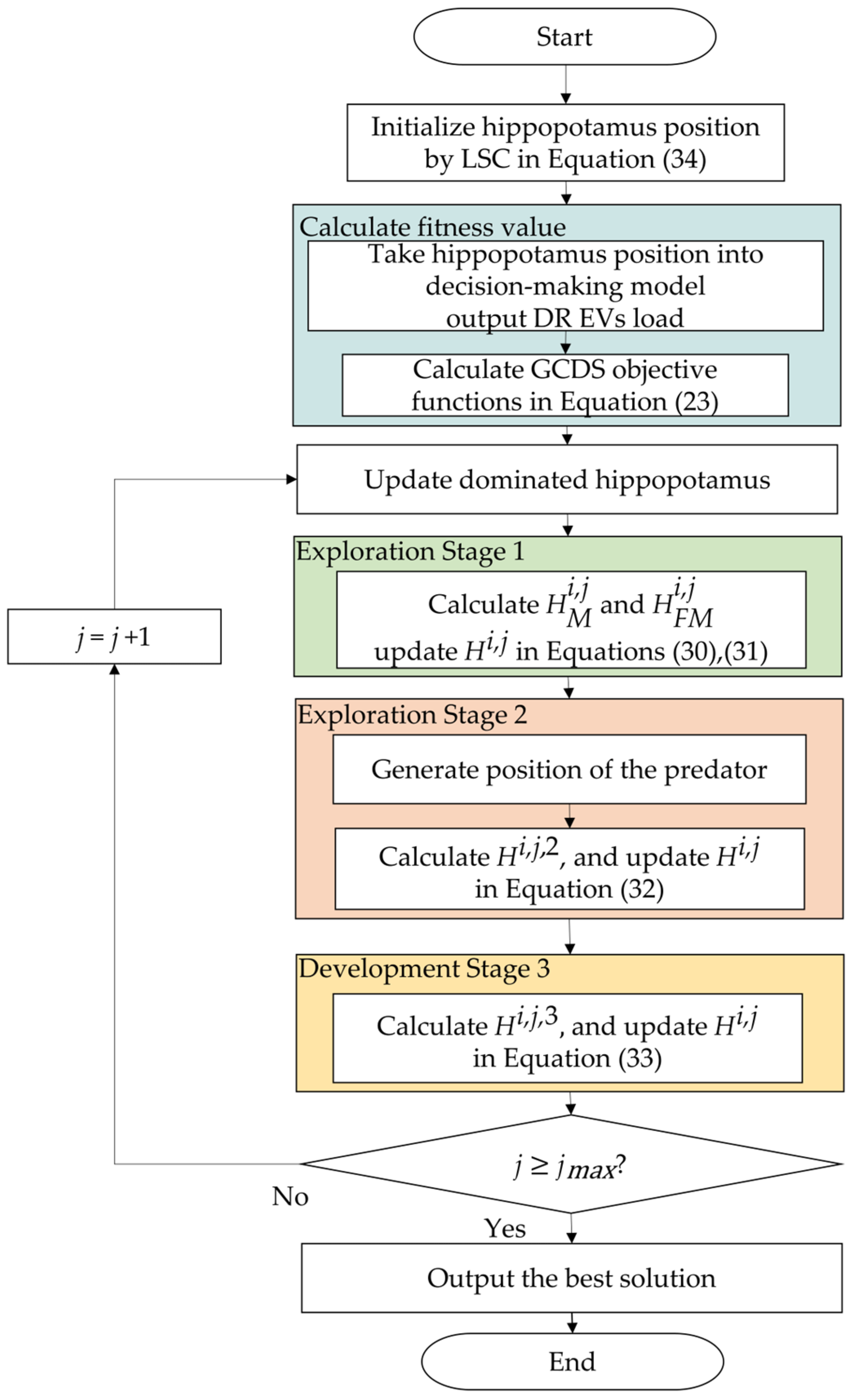
The LSC-HO flowchart is shown in Figure 4.

Step 1:

Set the LSO parameters, the maximum number, iterations, and the upper and lower limits;

Step 2:

Initialize the hippopotamus positions by LSC, output each hippopotamus, and calculate the initial value of the objective function;

Step 3:

Input the hippopotamus (tariffs), simulate the EVs DR charging/discharging load in that hippopotamus position, and calculate the value of the objective function;

Step 4:

According to the function value, update the hippopotamus position by Exploration stage 1, Exploration stage 2, and Development stage 3;

Step 5:

Determine whether the abort condition is reached or not, and if not, repeat Steps 3–4;

Step 6:

Output the best solution.

7. Results

7.1. Simulate System

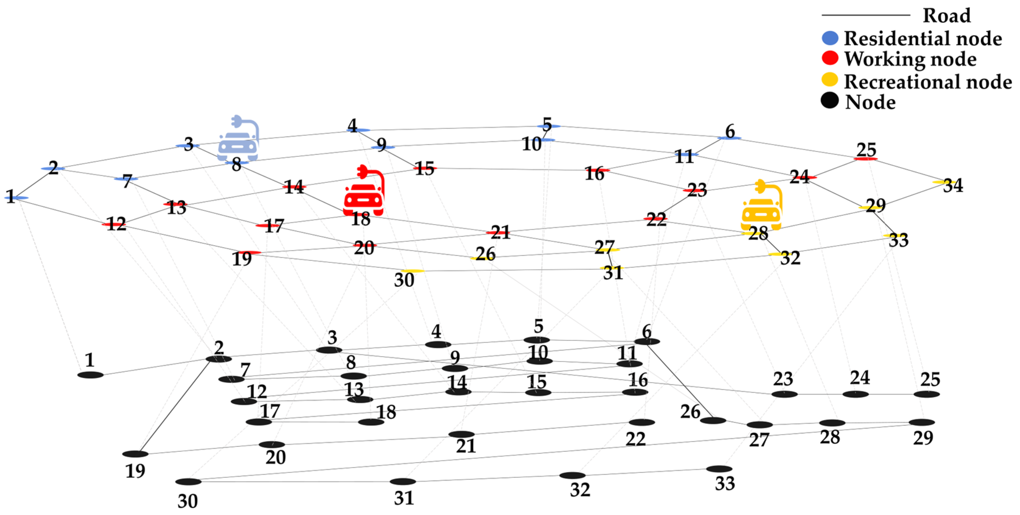
This study integrated a road network consisting of 34 nodes with an IEEE-33 distribution system. The coupling of these two networks allows us to analyze the interactions and dependencies between EVs traveling on the road network and their impact on the electric grid. The 34th node in the road network is a road network auxiliary node, which does not have electrical information, hence it is not shown in the IEEE-33. Figure 5 illustrates the modified IEEE-33 distribution system, where nodes 1–11 belong to the residential zone, nodes 12–25 belong to working zones, and nodes 26–34 belong to recreational zones.

7.2. Case Settings

This study considers the weekday scenario, which is dominated by the commuting chain, the number of total EVs is set to be 11,000. The proportion of EVs is set to be 7000 in the commuting chain, 2000 in the recreational chain for morning trips, and 2000 in the recreational chain for afternoon trips.

• The parameters are set as follows based on the statistics from [15,16,40,41,42]:
• ${\mu }_{t_{\mathit{id}}}$ is 10 and ${\sigma }_{t_{\mathit{id}}}$ is 2.0 in morning trip; ${\mu }_{t_{\mathit{id}}}$ is 16 and ${\sigma }_{t_{\mathit{id}}}$ is 1.8 in afternoon trip;
• ${\mu }_{T_{\mathit{pa}}}$, ${\sigma }_{T_{\mathit{pa}}}$, and ${\xi }_{T_{\mathit{pa}}}$ are set to be 360, 50, and 0.65 for parking time in the working zone, respectively; ${\mu }_{T_{\mathit{pa}}}$, ${\sigma }_{T_{\mathit{pa}}}$, and ${\xi }_{T_{\mathit{pa}}}$ are set to be 70, 45, and 0.65 for parking time in the recreational zone;
• ${\mu }_{{\mathit{SOC}}_{\mathit{id}}}$ is set to be 0.455, and ${\sigma }_{{\mathit{SOC}}_{\mathit{id}}}$ is set to be 0.1 for initial departure SOC;
• The weather is set to sunny;
• The EV charging power is 70 kW, and the EV battery capacity is 47.7 kWh. The charging and discharging efficiency are both 0.9.

The simulation interval is set to 1 min. The tariff-optimization interval is set to 60 min. The simulation duration is 24 h of a whole day. The upper and lower limits of SOC are set to be 0.9 and 0.1, respectively. The mileage anxiety threshold $\epsilon$ is set to be 0.25.

Table 1. Simulation cases.

Case	CDDR Scheduling	NDDR Scheduling	GCDS Scheduling	FTB Scheduling
Case 1
Case 2	√	√
Case 3	√	√	√
Case 4	√	√	√	√

gives the cases to verify the proposed method in this study.

This article did not use any commercial materials, and all simulations were conducted using Matlab R2022b software, made in MathWorks, manufactured by MathWorks, located in Natick, MA, USA.

7.3. Analysis of Algorithms

7.3.1. The Result of PV Output Prediction

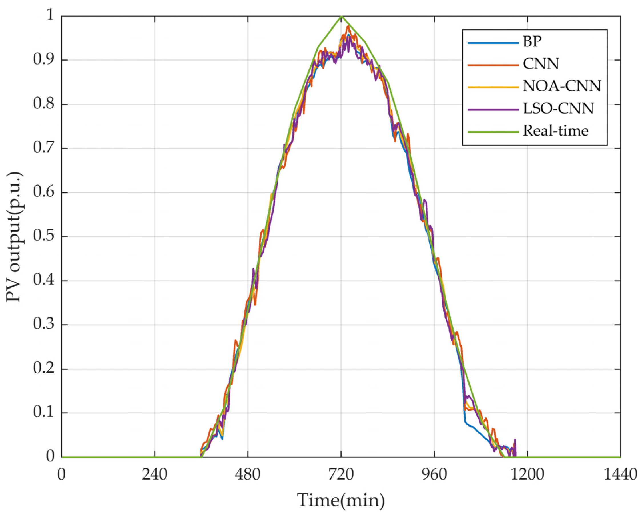
Figure 6 illustrates the comparison of PV output using the backpropagation neural network (BP), CNN, Nutcracker Optimization Algorithm (NOA)-CNN, and LSO-CNN. Based on their distinct characteristics and performance in the existing literature [7,8,9,10], the BPNN was selected as a benchmark due to its established effectiveness in PV output prediction tasks. The CNN, as the original algorithm, serves as a reference point for comparison with the improved versions. The NOA-CNN model was chosen for comparison with the LSO-CNN in the improved base on the original CNN. Finally, the LSO-CNN model represents a novel approach that integrates the LSO algorithm with the CNN for improved prediction accuracy. This comparative analysis provides a comprehensive overview of the performance of these models in predicting PV output, the inclusion of these diverse models allows for a thorough evaluation of the proposed approach against established and enhanced methods.

The population size for both the NOA and LSO is set to 50, with 200 iterations. The maximum number of epochs for the BPNN, CNN, NOA, and LSO are all set to 300. The results indicate that the RMSE of the LSO-CNN, as proposed in this study, is 39.2% lower than the BPNN, 24% lower than the original CNN, and 10.2% lower than the NOA-CNN. Therefore, the LSO-CNN has significantly enhanced the prediction accuracy of PV output.

7.3.2. Comparison of Optimization Algorithms

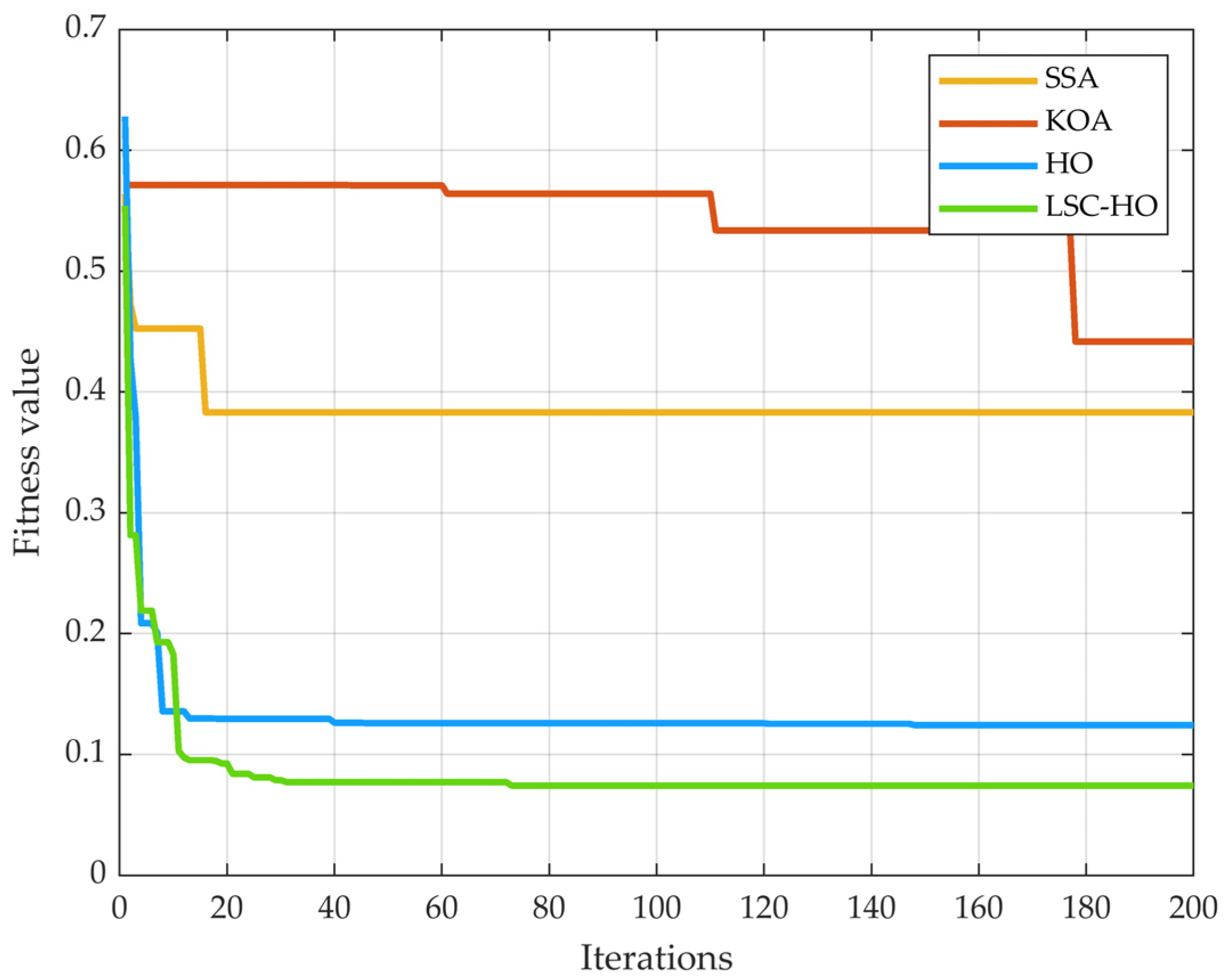
Figure 7 depicts the comparison of fitness convergence curves of the salp swarm algorithm (SSA), Kepler optimization algorithm (KOA), HO, and LSC-HO in tariff optimization. The algorithms were all operated on an Inte(R) Core (TM) i5-13500H 2.60 GHz CPU Thunderbot 911x made in Qingdao, China. The swarm size of each algorithm was set to 50, and the number of iterations was 200. The optimization completed time of LSC-HO was 54,042 s, that of the HO was 53,517 s, that of the SSA was 58746s, and that of the KOA was 46,967 s; at the same time, it can be seen in Figure 6 that the convergence accuracy of LSC-HO is better than that of HO 10.2%, SSA 68.3%, and KOA 73.4%. Therefore, LSC-HO is the comprehensively optimal algorithm.

7.4. Comparison of Case

7.4.1. Comparison of Charging/Discharging Distribution

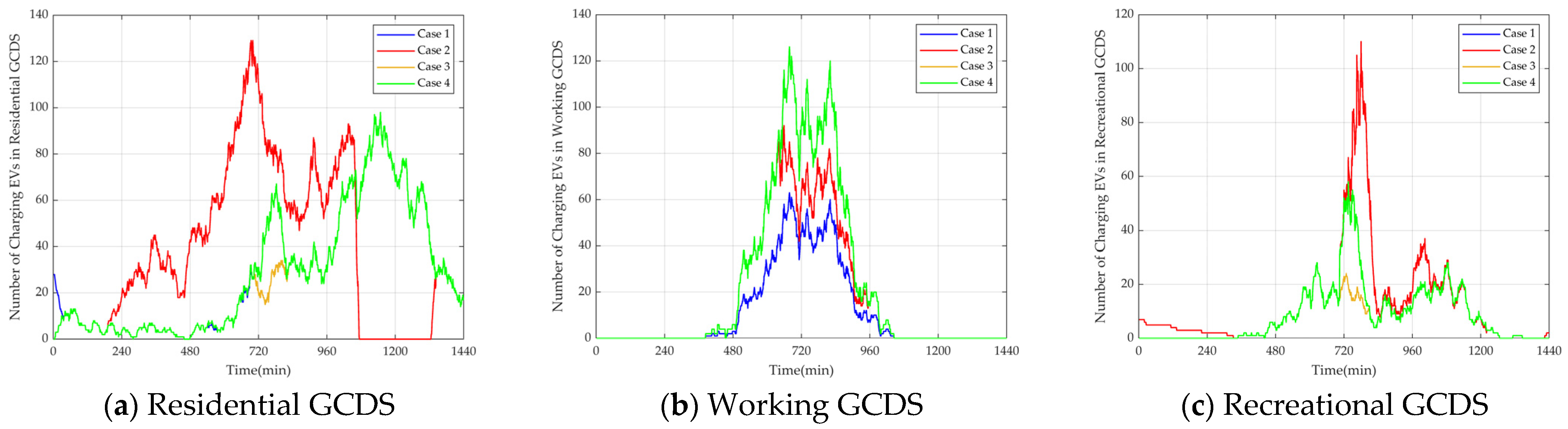
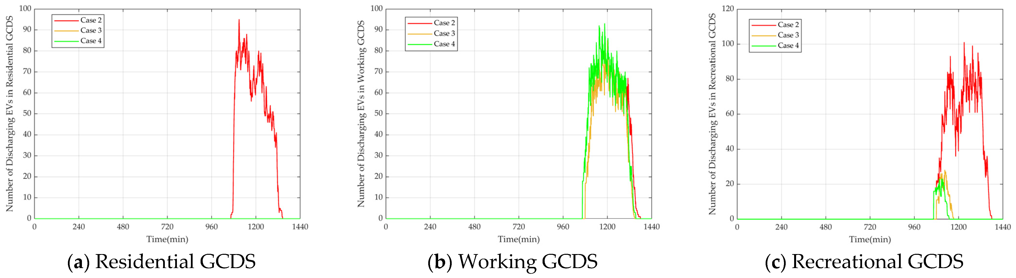
Figure 8 and Figure 9 depict the distribution of charging and discharging EVs. As shown in Figure 8a, Case 2 demonstrates a significant increase in the number of people charging during the daytime compared to Case 1, in order to balance PV output, while there is a notable decrease in the number of people charging during the 1000–1300 min period to avoid peak electricity usage. Case 3 and Case 4 do not have as good of scheduling abilities as Case 2. Figure 8b reveals that Case 4 and Case 3 have the highest number of people charging during the daytime, followed by Case 2, and Case 1 has the lowest number. The trend in Figure 8c is roughly similar to that in Figure 8a. Figure 9a shows that there are no discharging EVs at residential GCDS for Case 3 and Case 4, as charging EVs occupy the spots at the same time, preventing discharging EVs from participating. Figure 9b clearly indicates that Case 4 has more scheduled EVs than Case 3, but Case 2 has the most EVs and the longest final discharge time. Figure 9c shows that Case 3 and Case 4 only have a small number of discharging EVs. Therefore, by observing the overall distribution of charging and discharging EVs, it can be seen that Cases 2, 3, and 4 have significantly improved compared to Case 1, resulting in a more balanced distribution of charging and discharging EVs at the GCDS and enhancing the utilization rate of the GCDSs.

7.4.2. Comparison of Charging Cost and Discharging Profit

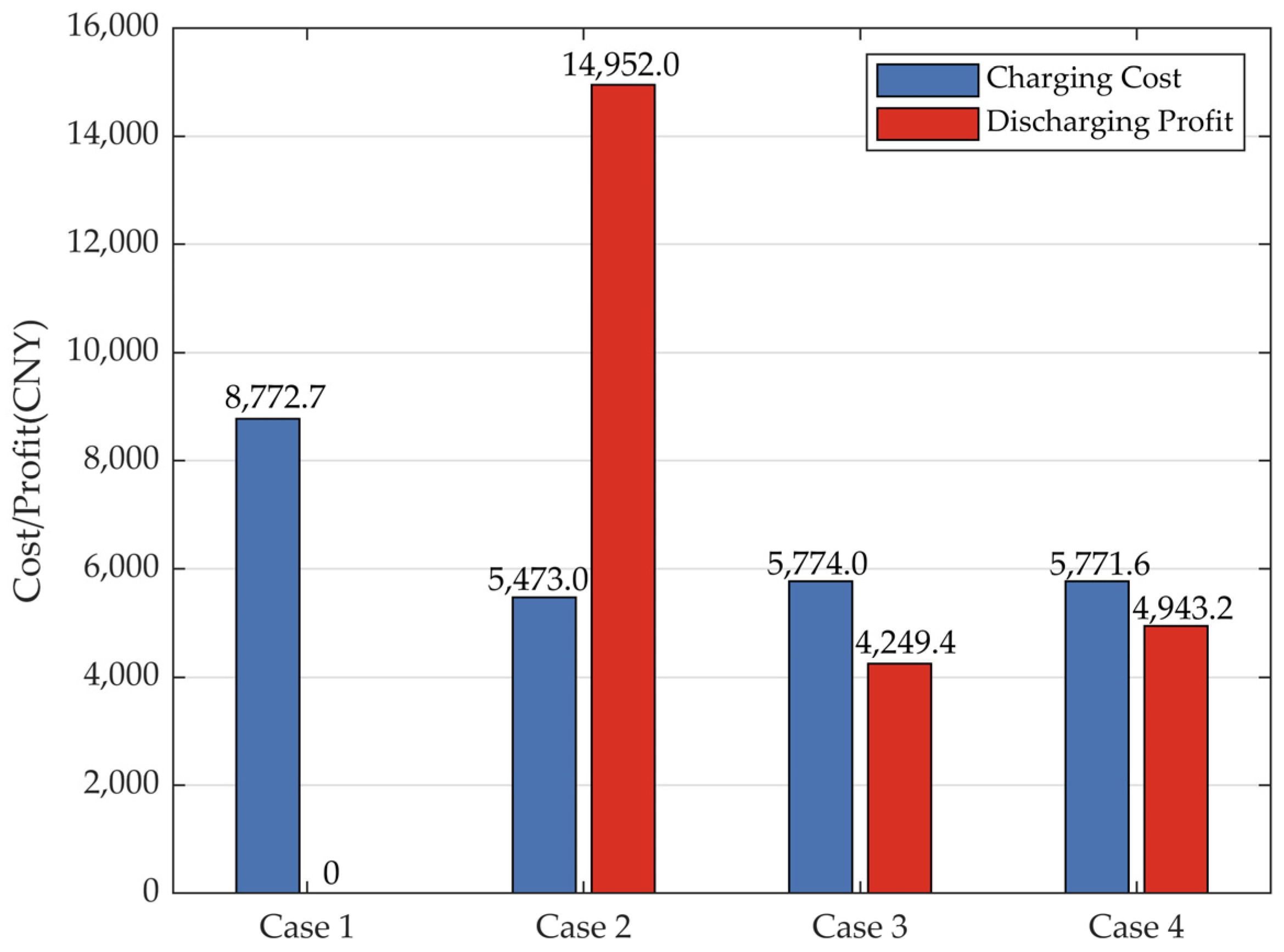
Figure 10 depicts the cost and profit of charging and discharging EVs. In Case 1, due to the absence of a scheduling strategy, there are only charging costs for EVs, totaling 8772.7 CNY, and no discharging EVs. In Cases 2, 3, and 4, the charging profit is calculated as the difference between the charging expenses in Case 1 and the charging costs in Cases 2, 3, and 4, respectively, while the discharging profit directly corresponds to the fees earned from discharging.

By comparing the charging costs across Cases 1, 2, 3, and 4, the results reveal that Case 1 has the highest charging prices, resulting in the highest charging costs for EVs. Case 2 shows the lowest charging prices, with a decrease of 37.6% compared to Case 1, followed by Case 3 with a 34.1% decrease, and Case 4 with a 34.2% decrease.

Furthermore, the analysis of discharging profits in Cases 2, 3, and 4 indicates that Case 2 has the highest discharging profit, suggesting a larger number of discharging EVs compared to the other scenarios. Conversely, Case 3 has the lowest discharging profit.

Overall, the comparison highlights the significant improvement in the scheduling strategy compared to uncoordinated charging. From the perspective of enhancing the efficiency, reliability, and sustainability of GCDSs, the objective is to maximize charging revenues and minimize discharging costs. Therefore, while Case 2 shows the highest discharging profit, it may not represent the optimal strategy. Instead, Cases 3 and 4 demonstrate a more optimal approach to achieving the objectives of enhancing the efficiency, reliability, and sustainability of GCDS.

7.4.3. Comparison of Voltage Quality

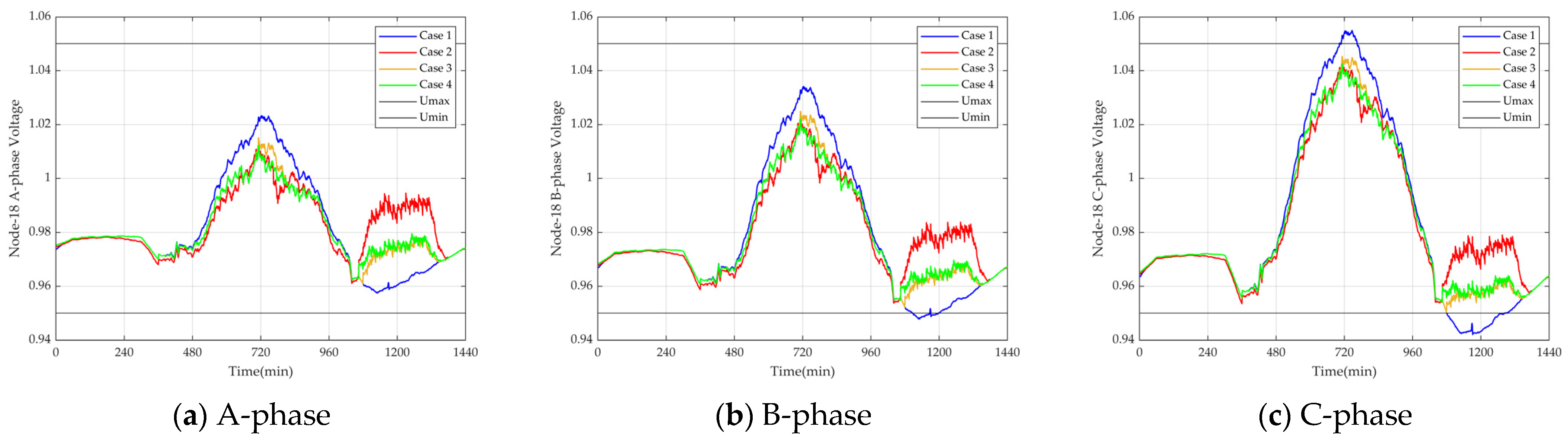
Figure 11 depicts the voltage of node 18 in each case.

Table 2. The voltage quality of each case.

	Case 1	Case 2	Case 3	Case 4
Voltage Exceeding Rate (p.u.)	0.1833	0	0	0
Voltage Fluctuation Rate (p.u.)	0.0294	0.0222	0.0248	0.0241

depicts voltage quality in each case. Node 18 is the terminal node with the worst power quality; therefore, the voltage situation at node 18 is presented. By comparing the three phases, it is evident that C-phase has the lowest voltage. It can be clearly seen from Figure 11c that in Case 1, there are instances of voltage exceeding both the upper and lower limits. Table 2 also shows that Case 1 has the highest voltage exceeding rate and voltage fluctuation rate. Cases 2, 3, and 4, through scheduling strategies, have significantly improved the voltage quality, preventing any voltage violations. Among them, Case 2 has the best voltage regulation capability which decreases the voltage fluctuation rate by 24.5%, followed by Case 4 which decreases the voltage fluctuation rate by 18.1%, and then Case 3 which decreases the voltage fluctuation rate by 15.6%. Taking into account both the GCDS and the EV side, despite Case 2 having higher power quality, its high discharging profit could result in the GCDS operating at a loss. Therefore, overall, Case 3 and Case 4 are currently the optimal strategies.

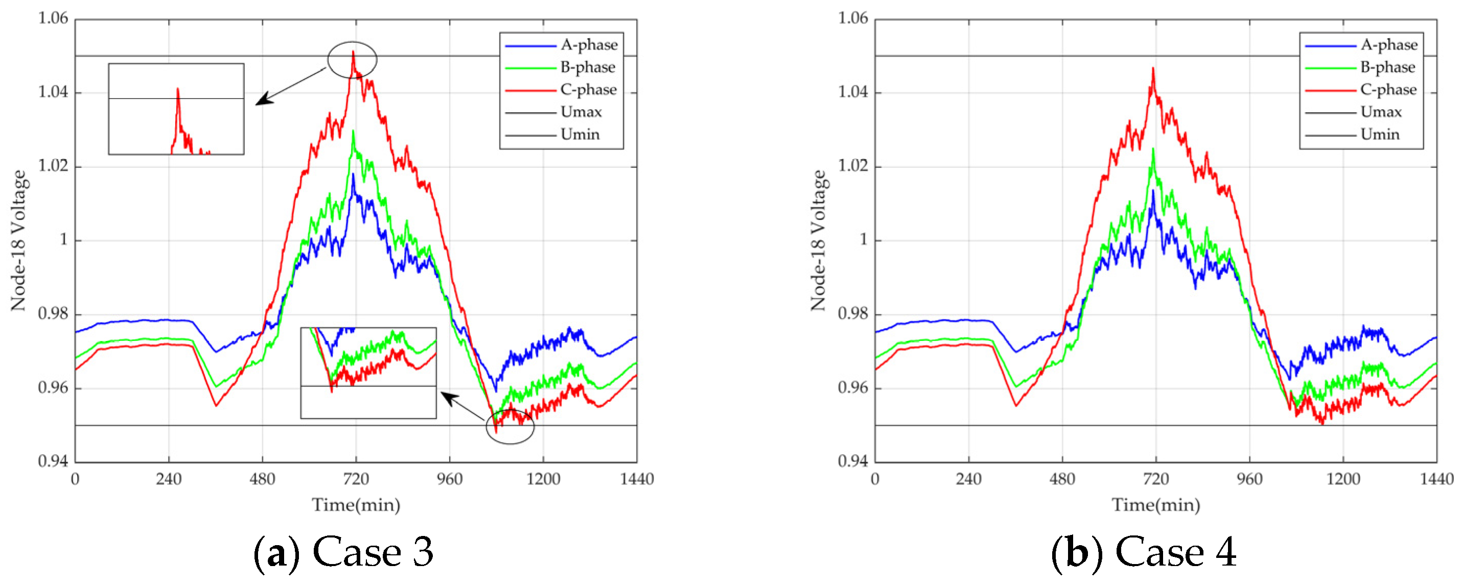
7.4.4. Incorporate Comprehensive Error

Figure 12 depicts the voltage quality incorporating comprehensive error. In this study, consider the PV forecasting error, EV forecasting error, as well as the scheduling errors of CDDR and NDDR, including defaults, timeouts, etc. By incorporating these errors into the updates, it can be observed that Case 3 experiences short-term voltage exceeding due to the absence of a threshold band. On the other hand, Case 4, aided by the FTB, effectively addresses these errors, ensuring no voltage exceedances occur.

Therefore, overall, Case 4 emerges as the optimal scheduling approach. It demonstrates the effectiveness of the anchoring effect CDDR and regret theory NDDR decision-making model proposed in this paper, which ensures EV profits. Furthermore, it also demonstrates the effectiveness of the EV charging margin and FTB model, which ensures GCDS voltage quality and revenue and equips this strategy to handle various forecasting and operational errors.

7.4.5. Finalized Case Comparison

Table 3. The finalized comparison with Case 1.

Case Compares with Case 1	Charging Costs (Yuan)	Discharging Profits (Yuan)	Voltage Exceeding Rate (p.u.)	Voltage Fluctuation Rate (p.u.)
Case 2	−3299.7	+14,952.0	−18.33	−0.72
Case 3	−2998.7	+4249.4	−18.33	−0.98
Case 4	−3001.1	+4349.2	−18.33	−0.91

presents the results of each case compared to Case 1. In terms of reducing charging costs, Case 2 shows the most significant decrease as shown in Table 3, demonstrating the effectiveness of the approach in reducing charging costs. From the perspective of increasing EV discharging profits, Case 2 exhibits the most substantial increase.

Regarding the reduction in voltage exceeding rate, none of the scenarios (Case 2, Case 3, or Case 4) experienced voltage exceeding, confirming the effectiveness of their methods in reducing voltage exceeding. Case 3 demonstrates the most significant reduction in voltage fluctuation, further validating the effectiveness of its approach in reducing voltage fluctuations. Considering the impact of errors, Case 4 performs the best. Despite a brief voltage violation in Case 3, this also demonstrates the effectiveness of the approach in addressing such occurrences.

In summary, from an EV perspective, Case 2 is a relatively excellent choice. However, for the satisfaction of both the EV and the GCDS, Case 3 and Case 4 are more favorable. Given the potential occurrence of various errors, it is essential to consider this factor. Case 4 can effectively handle these errors, making the method in Case 4 the optimal choice. Therefore, by comprehensively considering the anchoring effect CDDR and regret theory NDDR decision-making model, the EVs charging margin model, and the FTB model, it can improve the satisfaction of both EVs and GCDSs.

8. Conclusions

The rapid growth of EVs, GCDSs, and related infrastructure has made it challenging to sustainably utilize EV charging loads and flexible resources. This randomness presents challenges to the reliability and sustainability of distribution networks, highlighting the need to develop efficient charging and discharging scheduling strategies in electric vehicle dispatch research. To tackle the sustainable utilization of EV and flexibility resources, the proposed model utilizes the LSO-CNN to predict the PV output and employs Monte Carlo simulation to estimate the charging load of EVs, ensuring accurate PV output prediction and efficient EV distribution. To tackle the stochastic nature of EV charging loads and enhance EV owners’ satisfaction, we propose the anchoring effect CDDR and regret theory NDDR decision-making models, which take into account the satisfaction of EVs. Then, to enhance the efficiency, reliability, and sustainability of DNs, we propose the EV charging margin model and FTB model to solve the optimal satisfaction of both EV and GCDSs with the LSC-HO.

In this paper, the LSO-CNN prediction algorithm is proposed, which shows a significant improvement in PV prediction accuracy, and the prediction RMSE is 39.2% lower than the BPNN, 24% lower than the original CNN, and 10.2% lower than the NOA-CNN, thus ensuring accurate PV output prediction to tackle the sustainable utilization of PV.

The anchoring effect CDDR and regret theory NDDR decision-making model, the EVs charging margin model, and the FTB model proposed in this paper improve the satisfaction of both EVs and GFCSs. In terms of EVs, which decreased by 34.2% in charging cost and increased by 4943.2 CNY in discharging profit, we effectively addressed the stochastic nature of EV charging loads and enhanced EV owners’ satisfaction. In terms of GCDSs, which decreased in voltage fluctuation rate by 18.1%, we prevented voltage exceeding and effectively addressed errors, effectively enhancing the efficiency, reliability, and sustainability of DNs.

The LSC-HO optimization algorithm has the advantage of faster convergence; the results verify that the final convergence fitness value is the smallest, and the convergence accuracy of LSC-HO is better than that of HO 10.2%, SSA 68.3%, and KOA 73.4%, thereby improving the sustainable utilization and scheduling efficiency of EVs and flexibility resources.

This study offers DR strategies to optimize the utilization of charging infrastructure and improve EV charging plans. It aims to address the evolving needs of the public for EV charging facilities. The research outcomes not only provide insights for businesses but also offer decision-making guidance for policymakers. Governments and urban planners can leverage these findings to enhance the stability, safety, and compatibility of GCDSs during deployment.

In addition, further work needs to be carried out. Firstly, enhancing the accuracy of predicting the spatial distribution of EVs by utilizing spatiotemporal coupling factors needs to be completed. Secondly, proposing a more precise grid–road network coupling model to improve scheduling accuracy and applicability should be performed. Lastly, evaluating the effectiveness of scheduling strategies in large-scale systems or interconnected regional systems needs to be conducted. These tasks are currently ongoing as part of our research.

References

- Hu, R.; Cai, T.; Xu, W. Exploring the Technology Changes of New Energy Vehicles in China: Evolution and Trends. Comput. Ind. Eng. 2024, 191, 110178. [Google Scholar] [CrossRef]
- Chen, X.H.; Tee, K.; Elnahass, M.; Ahmed, R. Assessing the Environmental Impacts of Renewable Energy Sources: A Case Study on Air Pollution and Carbon Emissions in China. J. Environ. Manag. 2023, 345, 118525. [Google Scholar] [CrossRef] [PubMed]
- National Energy Administration. The National Energy Administration Convened the National Renewable Energy Development and Construction Scheduling Meeting for September 2024. Available online: https://www.nea.gov.cn/2024-10/09/c_1310786347.htm (accessed on 9 October 2024).
- Huang, W.; Wang, J.; Wang, J.; Zhou, M.; Cao, J.; Cai, L. Capacity Optimization of PV and Battery Storage for EVCS with Multi-Venues Charging Behavior Difference towards Economic Targets. Energy 2024, 313, 133833. [Google Scholar] [CrossRef]
- Rehman, A.U.; Ullah, Z.; Shafiq, A.; Hasanien, H.M.; Luo, P.; Badshah, F. Load Management, Energy Economics, and Environmental Protection Nexus Considering PV-Based EV Charging Stations. Energy 2023, 281, 128332. [Google Scholar] [CrossRef]
- Sun, F.; Diao, R.; Zhou, B.; Lan, T.; Mao, T.; Su, S.; Cheng, H.; Meng, D.; Lu, S. Prediction-Based EV-PV Coordination Strategy for Charging Stations Using Reinforcement Learning. IEEE Trans. Ind. Appl. 2024, 60, 910–919. [Google Scholar] [CrossRef]
- Scott, C.; Ahsan, M.; Albarbar, A. Machine Learning for Forecasting a Photovoltaic (PV) Generation System. Energy 2023, 278, 127807. [Google Scholar] [CrossRef]
- Kumar Ganti, P.; Naik, H.; Kanungo Barada, M. Environmental Impact Analysis and Enhancement of Factors Affecting the Photovoltaic (PV) Energy Utilization in Mining Industry by Sparrow Search Optimization Based Gradient Boosting Decision Tree Approach. Energy 2022, 244, 122561. [Google Scholar] [CrossRef]
- Wu, S.; Guo, H.; Zhang, X.; Wang, F. Short-Term Photovoltaic Power Prediction Based on CEEMDAN and Hybrid Neural Networks. IEEE J. Photovolt. 2024, 14, 960–969. [Google Scholar] [CrossRef]
- Abou Houran, M.; Salman Bukhari, S.M.; Zafar, M.H.; Mansoor, M.; Chen, W. COA-CNN-LSTM: Coati Optimization Algorithm-Based Hybrid Deep Learning Model for PV/Wind Power Forecasting in Smart Grid Applications. Appl. Energy 2023, 349, 121638. [Google Scholar] [CrossRef]
- Ren, X.; Zhang, F.; Zhu, H.; Liu, Y. Quad-Kernel Deep Convolutional Neural Network for Intra-Hour Photovoltaic Power Forecasting. Appl. Energy 2022, 323, 119682. [Google Scholar] [CrossRef]
- Wang, L.; Mao, M.; Xie, J.; Liao, Z.; Zhang, H.; Li, H. Accurate Solar PV Power Prediction Interval Method Based on Frequency-Domain Decomposition and LSTM Model. Energy 2023, 262, 125592. [Google Scholar] [CrossRef]
- Mahmoudi, E.; dos Santos Barros, T.A.; Filho, E.R. Forecasting Urban Electric Vehicle Charging Power Demand Based on Travel Trajectory Simulation in the Realistic Urban Street Network. Energy Rep. 2024, 11, 4254–4276. [Google Scholar] [CrossRef]
- Yin, W.; Ji, J. Research on EV Charging Load Forecasting and Orderly Charging Scheduling Based on Model Fusion. Energy 2024, 290, 130126. [Google Scholar] [CrossRef]
- Liu, K.; Liu, Y. Stochastic User Equilibrium Based Spatial-Temporal Distribution Prediction of Electric Vehicle Charging Load. Appl. Energy 2023, 339, 120943. [Google Scholar] [CrossRef]
- Shen, H.; Wang, Z.; Zhou, X.; Lamantia, M.; Yang, K.; Chen, P.; Wang, J. Electric Vehicle Velocity and Energy Consumption Predictions Using Transformer and Markov-Chain Monte Carlo. IEEE Trans. Transp. Electrif. 2022, 8, 3836–3847. [Google Scholar] [CrossRef]
- Lu, J.; Yin, W.; Wang, P.; Ji, J. EV Charging Load Forecasting and Optimal Scheduling Based on Travel Characteristics. Energy 2024, 311, 133389. [Google Scholar] [CrossRef]
- Lin, R.; Xu, Z.; Huang, X.; Gao, J.; Chen, H.; Shen, T. Optimal Scheduling Management of the Parking Lot and Decentralized Charging of Electric Vehicles Based on Mean Field Game. Appl. Energy 2022, 328, 120198. [Google Scholar] [CrossRef]
- Zhao, Z.; Lee, C.K.M.; Ren, J. A Two-Level Charging Scheduling Method for Public Electric Vehicle Charging Stations Considering Heterogeneous Demand and Nonlinear Charging Profile. Appl. Energy 2024, 355, 122278. [Google Scholar] [CrossRef]
- Zhou, K.; Cheng, L.; Wen, L.; Lu, X.; Ding, T. A Coordinated Charging Scheduling Method for Electric Vehicles Considering Different Charging Demands. Energy 2020, 213, 118882. [Google Scholar] [CrossRef]
- Liu, L.; Zhou, K. Electric Vehicle Charging Scheduling Considering Urgent Demand under Different Charging Modes. Energy 2022, 249, 123714. [Google Scholar] [CrossRef]
- Aghajan-Eshkevari, S.; Azad, S.; Nazari-Heris, M.; Ameli, M.T.; Asadi, S. Charging and Discharging of Electric Vehicles in Power Systems: An Updated and Detailed Review of Methods, Control Structures, Objectives, and Optimization Methodologies. Sustainability 2022, 14, 2137. [Google Scholar] [CrossRef]
- Wu, H.; Lan, X.; He, Y.; Wu, A.Y.; Ding, M. Orderly Charging of Electric Vehicles: A Two-Stage Spatial-Temporal Scheduling Method Based on User-Personalized Navigation. Appl. Energy 2025, 378, 124800. [Google Scholar] [CrossRef]
- Phipps, K.; Schwenk, K.; Briegel, B.; Mikut, R.; Hagenmeyer, V. Customized Uncertainty Quantification of Parking Duration Predictions for EV Smart Charging. IEEE Internet Things J. 2023, 10, 20649–20661. [Google Scholar] [CrossRef]
- Wu, F.; Yang, J.; Li, B.; Crisostomi, E.; Rafiq, H.; Rashed, G.I. Uncertain Scheduling Potential of Charging Stations under Multi-Attribute Uncertain Charging Decisions of Electric Vehicles. Appl. Energy 2024, 374, 124036. [Google Scholar] [CrossRef]
- Zhang, K.; Xu, Y.; Sun, H. Bilevel Optimal Coordination of Active Distribution Network and Charging Stations Considering EV Drivers’ Willingness. Appl. Energy 2024, 360, 122790. [Google Scholar] [CrossRef]
- Liu, J.; Lin, G.; Huang, S.; Zhou, Y.; Li, Y.; Rehtanz, C. Optimal EV Charging Scheduling by Considering the Limited Number of Chargers. IEEE Trans. Transp. Electrif. 2021, 7, 1112–1122. [Google Scholar] [CrossRef]
- Qureshi, U.; Ghosh, A.; Panigrahi, B.K. Menu-Based Pricing for Electric Vehicle Charging in a Mobile Charging Service for Maximizing Charging Station’s Profit and Social Welfare: A Stackelberg Game. IEEE Trans. Ind. Appl. 2024, 1–10. [Google Scholar] [CrossRef]
- Wu, J.; Su, H.; Meng, J.; Lin, M. Electric Vehicle Charging Scheduling Considering Infrastructure Constraints. Energy 2023, 278, 127806. [Google Scholar] [CrossRef]
- Obeid, H.; Ozturk, A.T.; Zeng, W.; Moura, S.J. Learning and Optimizing Charging Behavior at PEV Charging Stations: Randomized Pricing Experiments, and Joint Power and Price Optimization. Appl. Energy 2023, 351, 121862. [Google Scholar] [CrossRef]
- Qureshi, U.; Ghosh, A.; Panigrahi, B.K. Multiobjective Pareto-Optimal Intelligent Electric Vehicle Charging Schedule in a Commercial Charging Station: A Stochastic Convex Optimization Approach. IEEE Trans. Ind. Inform. 2024, 20, 12620–12632. [Google Scholar] [CrossRef]
- Kandpal, B.; Pareek, P.; Verma, A. A Robust Day-Ahead Scheduling Strategy for EV Charging Stations in Unbalanced Distribution Grid. Energy 2022, 249, 123737. [Google Scholar] [CrossRef]
- Feng, J.; Ran, L.; Wang, Z.; Zhang, M. Optimal Energy Scheduling of Virtual Power Plant Integrating Electric Vehicles and Energy Storage Systems under Uncertainty. Energy 2024, 309, 132988. [Google Scholar] [CrossRef]
- Sifakis, N.K.; Kanellos, F.D. Real-Time Multi-Agent Based Power Management of Virtually Integrated Microgrids Comprising Prosumers of Plug-in Electric Vehicles and Renewable Energy Sources. IEEE Access 2024, 12, 161842–161865. [Google Scholar] [CrossRef]
- Jiao, F.; Zou, Y.; Zhang, X.; Zhang, B. Online Optimal Dispatch Based on Combined Robust and Stochastic Model Predictive Control for a Microgrid Including EV Charging Station. Energy 2022, 247, 123220. [Google Scholar] [CrossRef]
- Gaboitaolelwe, J.; Zungeru, A.M.; Yahya, A.; Lebekwe, C.K.; Vinod, D.N.; Salau, A.O. Machine Learning Based Solar Photovoltaic Power Forecasting: A Review and Comparison. IEEE Access 2023, 11, 40820–40845. [Google Scholar] [CrossRef]
- Suresh, V.; Janik, P.; Rezmer, J.; Leonowicz, Z. Forecasting Solar PV Output Using Convolutional Neural Networks with a Sliding Window Algorithm. Energies 2020, 13, 723. [Google Scholar] [CrossRef]
- Abdel-Basset, M.; Mohamed, R.; Sallam, K.M.; Chakrabortty, R.K. Light Spectrum Optimizer: A Novel Physics-Inspired Metaheuristic Optimization Algorithm. Mathematics 2022, 10, 3466. [Google Scholar] [CrossRef]
- Deng, Z.; Wang, H.; Liu, H.; Chen, Q.; Zhang, J. Degradation Prediction of Proton Exchange Membrane Fuel Cell Using a Novel Neuron-Fuzzy Model Based on Light Spectrum Optimizer. Renew. Energy 2024, 234, 121192. [Google Scholar] [CrossRef]
- Yan, Q.; Gao, Y.; Xing, L.; Xu, B.; Li, Y.; Chen, W. Optimal Scheduling for Increased Satisfaction of Both Electric Vehicle Users and Grid Fast-Charging Stations by SOR&KANO and MVO in PV-Connected Distribution Network. Energies 2024, 17, 3413. [Google Scholar] [CrossRef]
- Mirzahossein, M.; Mashhadloo, M. Modeling the Effect of Autonomous Vehicles (AVs) on the Accessibility of the Transportation Network. Sci. Rep. 2024, 14, 9292. [Google Scholar] [CrossRef]
- The People’s Government of Henan Province. Implementation Plan for Accelerating the Development of New Energy Vehicles in Henan Province. Available online: https://www.henan.gov.cn/2022/05-19/2451587.html (accessed on 19 May 2022).
- Liu, Y.; Tian, J.; Yu, N. Emergency Supplies Prepositioning via a Government-Led Supply Chain with a Loss-Averse Supplier with Anchoring. Comput. Ind. Eng. 2023, 182, 109362. [Google Scholar] [CrossRef]
- Seo, Y.-D.; Cho, Y.-S. Point of Interest Recommendations Based on the Anchoring Effect in Location-Based Social Network Services. Expert Syst. Appl. 2021, 164, 114018. [Google Scholar] [CrossRef]
- Wang, P. Pricing Innovation: The Anchoring Effect in Patent Valuation. Technovation 2024, 136, 103070. [Google Scholar] [CrossRef]
- Pan, X.-H.; Wang, Y.-M.; He, S.-F. A New Regret Theory-Based Risk Decision-Making Method for Renewable Energy Investment under Uncertain Environment. Comput. Ind. Eng. 2022, 170, 108319. [Google Scholar] [CrossRef]
- Wang, Y.-M.; Jia, X.; Song, H.-H.; Martínez, L. Improving Consistency Based on Regret Theory: A Multi-Attribute Group Decision Making Method with Linguistic Distribution Assessments. Expert. Syst. Appl. 2023, 221, 119748. [Google Scholar] [CrossRef]
- Li, F.; Du, X.; Li, H.; Huang, X.; Fei, X. Study on Household Investment Decision of Household Photovoltaic Project Promotion-Based on Inclusive Finance Perspective. J. Clean. Prod. 2024, 482, 144185. [Google Scholar] [CrossRef]
- Amiri, M.H.; Mehrabi Hashjin, N.; Montazeri, M.; Mirjalili, S.; Khodadadi, N. Hippopotamus Optimization Algorithm: A Novel Nature-Inspired Optimization Algorithm. Sci. Rep. 2024, 14, 5032. [Google Scholar] [CrossRef]
- Maurya, P.; Tiwari, P.; Pratap, A. Application of the Hippopotamus Optimization Algorithm for Distribution Network Reconfiguration with Distributed Generation Considering Different Load Models for Enhancement of Power System Performance. Electr. Eng. 2024. [Google Scholar] [CrossRef]
- Abdelaziz, M.A.; Ali, A.A.; Swief, R.A.; Elazab, R. Optimizing Energy-Efficient Grid Performance: Integrating Electric Vehicles, DSTATCOM, and Renewable Sources Using the Hippopotamus Optimization Algorithm. Sci. Rep. 2024, 14, 28974. [Google Scholar] [CrossRef]
- Demir, F.B.; Tuncer, T.; Kocamaz, A.F. A Chaotic Optimization Method Based on Logistic-Sine Map for Numerical Function Optimization. Neural Comput. Appl. 2020, 32, 14227–14239. [Google Scholar] [CrossRef]
- Wang, M.; Wang, X.; Wang, C.; Zhou, S.; Xia, Z.; Li, Q. Color Image Encryption Based on 2D Enhanced Hyperchaotic Logistic-Sine Map and Two-Way Josephus Traversing. Digit. Signal Process. 2023, 132, 103818. [Google Scholar] [CrossRef]