Abstract
Driven by climate change and rapid urbanization, pluvial flooding is increasingly endangering urban environments, prompting the widespread use of coupled hydrological–hydrodynamic models that enable more accurate urban flood simulations and enhanced pluvial flood forecasting. The simulation method for urban river flooding caused by heavy rainfall has garnered growing attention. However, existing studies primarily concentrate on prediction using hydrodynamic models or machine learning models, and there remains a dearth of a comprehensive prediction framework that couples both models to simulate the temporal evolution of river flood changes. This research proposes a novel framework for simulating urban pluvial river flooding by integrating physically based models with deep learning approaches. The sample set is enhanced through data augmentation and Generative Adversarial Networks, and scheduling control signals are incorporated into the encoder–decoder architecture to enable urban pluvial river flooding forecasting. The results demonstrate strong model performance, provided that the model’s structural complexity is aligned with the available training data. After incorporating scheduling information, the simulated water level process exhibits a “double-peak” pattern, where the first peak is noticeably lower than that under non-scheduling conditions. The current research introduces an innovative method for simulating and analyzing large-scale urban flooding, offering valuable perspectives for urban planning and flood mitigation strategies.
1. Introduction
Climate change has the potential to induce extreme rainfall events and continually shifting precipitation patterns, exerting profound impacts on natural hydrological processes [1,2]. The constantly changing climate and ever-increasing urbanization have made flooding the most challenging issue faced by cities; these changes can lead to increased occurrences of urban flooding disasters, with adverse implications for existing urban infrastructure [3,4,5,6,7]. On 21 July 2012, extreme rainfall in Beijing resulted in the collapse of 10,660 houses, causing an economic loss of 1.83 billion US dollars [8]. On 20 July 2021, Zhengzhou city experienced an extreme rainfall event with a maximum hourly precipitation of 201.9 mm, leading to significant casualties and economic losses [9]. On 8 August 2015, Typhoon “Soudelor” made landfall in Fuzhou, resulting in prolonged heavy rainfall that caused severe damage to the economy and transportation infrastructure. It was the largest rainfall event in the history of Fuzhou city [10].
Urban flooding results from both natural events and human activities [11,12]. Urban areas are nested within larger-scale watersheds, where flood processes are subject to the dual influence of natural and anthropogenic factors [13,14]. Intensive urbanization in densely populated regions leads to an evolving impermeable surface pattern and expanding urban land cover over the years. Inadequate drainage capacity and insufficient maintenance of drainage infrastructure collectively alter the hydrodynamic characteristics of urban areas [15]. Coupled with the limited capacity of drainage systems to effectively handle short-term or continuous rainfall, these factors serve as significant drivers of urban flooding [16,17]. Frequent urban flooding disasters directly or indirectly lead to a range of societal losses, encompassing human and economic dimensions [18,19]. These losses notably include damage to public utility infrastructure, loss of household assets, and reductions in revenue within the industrial and transportation sectors [20]. Urban infrastructure’s flood control and drainage measures constitute essential technical means for addressing the latent threat posed by extreme rainfall-induced flood disasters. This multifaceted hydraulic engineering encompasses pipeline networks, reservoirs, embankments, retention basins, pumping stations, and other components, efficiently regulating river and lake water levels, while optimizing water discharge pathways and volumes. Consequently, these measures play a pivotal role in mitigating flood disasters triggered by heavy rainfall events.
Urban flood models play a pivotal role in aiding users to gain insight into, assess, and predict flood scenarios and their repercussions. Effectively conducting flood modeling, particularly within highly urbanized flood-prone regions, presents a challenge in the careful selection of models that align with environmental prerequisites [21]. Traditionally, the use of hydrologic models and the use of hydraulic models have been relatively independent. Hydrologic models are designed to address larger-scale dynamic water cycles, while hydraulic models are suited for fine-scale simulations at smaller spatial resolutions. Nevertheless, recent research, primarily in the domain of modeling intricate multi-physical processes associated with urban flooding, has frequently incorporated the integration of these two modeling methods [22]. A one-dimensional hydrodynamic model has been developed to simulate dynamic drainage processes in hydraulic elements such as pipelines, channels, and other hydrological components with fixed flow directions [23]. Two-dimensional hydrodynamic models are commonly employed to simulate depth and horizontal velocity distribution processes on urban surfaces, rivers, and lakes [24]. Hydrodynamic–hydrological coupling models seamlessly link early-stage rainfall and runoff processes with river and urban drainage network flow simulations. These models also allow for appropriate simplifications of certain complex physical processes. For instance, in cases where there is a significant disparity in spatial scales, such as open-channel flow with varying directions, simplified one-dimensional hydraulic models can be employed as alternatives. This integrated and systematic modeling approach provides a more realistic representation of the complete flood cascade, capturing the interactions between surface runoff, river flow, and urban drainage systems. The approach of combining hydrological and hydrodynamic models has strong interpretability, but it often requires high-resolution foundational data and substantial computational resources, making it widely used in urban flood modeling [10,16].
Although the traditional physics-based models have been the cornerstone of flood simulation for decades, they often face limitations in handling the complexity and nonlinearity of urban hydrological processes. Urban flood modeling involves complex, nonlinear hydraulic and physical processes. Recent research on urban flood simulation has witnessed a transformative shift with the adoption of machine learning and deep learning techniques [25,26,27,28]. Compared to physics-based numerical models, data-driven methods provide a powerful and flexible modeling approach, utilizing extensive datasets to enhance the accuracy and adaptability of flood prediction. Importantly, these data-driven methods do not rely on the nonlinear dynamic processes of multiple subsystems within urban flooding [29]. Machine learning and deep learning techniques excel at capturing complex hidden patterns within the rainfall–runoff relationship, offering efficient and accurate predictions for intricate urban drainage systems [30,31,32]. A wide range of data types is extensively utilized for modeling urban pluvial flooding. Intelligent algorithms are employed to generate flood simulation datasets, which encompass various types of data, broadly categorized into structured and unstructured data components [33]. Specifically, monitored meteorological and rainfall data exhibit structured one-dimensional characteristics, while geographical data, such as terrain and land use, possess structured spatial features, which are used to determine the underlying urban surface structure [34,35,36]. Recently, logistic regression [37,38], artificial neural networks [39,40], support vector machines [41,42], and random forests [43,44] have been extensively employed in urban flood risk assessment. As the sample size increases and the complexity of the problem grows, deep neural networks can automatically learn feature representations layer by layer, and extract abstract and advanced features from raw data [34,45,46]. The combination of physically based models and data-driven models plays a pivotal role, particularly when utilizing deep learning architectures like convolutional neural networks and recurrent neural networks. These deep learning frameworks provide the flexibility to enhance the structure of flood prediction models, thereby elevating simulation accuracy.
Consequently, this research aims to propose a framework for fusing a mechanism-driven model and data-driven model for accurately making regional multistep-ahead urban network flood forecasts. The key innovations of this research include the following:
- (a)
- A dataset suitable for deep learning simulations was generated based on a physically based model, and data augmentation was implemented using Generative Adversarial Networks (GANs).
- (b)
- Various deep learning models applicable to urban pluvial river flooding were developed based on an encoder–decoder framework. The performance of these models and the impact of model parameters were evaluated, with the relationship between data volume and model complexity explored.
- (c)
- The capture of scheduling signals in urban pluvial river flooding was achieved, fitting the nonlinear effects of water engineering scheduling signals.
2. Methodology
2.1. Procedural Modeling
We have developed an analytical framework known as Deep-River, and the framework continues to employ an object-oriented programming approach, enabling an “end-to-end” analysis of the model. The framework accomplishes four primary functions: (1) Hydro–hydraulic coupling: We establish a hydro–hydraulic coupled model based on factors influencing riverine floods, constructing datasets that include data on rainfall, upstream catchment runoff, reservoir discharge, and river water level processes. (2) Feature representation: Effective feature embedding and encoding significantly impact model performance. We employ a one-hot encoding pattern for rainfall and upstream catchment features. (3) Data augmentation module: Leveraging GAN models, we implement data augmentation to address deficiencies in hydrological data. This enables the model to learn more hidden patterns. (4) Encoder–decoder architecture: We design a multi-layer bidirectional recurrent neural network based on an encoder–decoder architecture to capture the time dependency of water levels. (5) Attention mechanism: The introduction of a self-attention mechanism extends the model’s ability to extract temporal features. The workflow of this study is shown in Figure 1.

Figure 1.
Study workflow.
2.2. Physically Based Model (PBM)
During intense urban rainfall events, evaporation and interception can be reasonably simplified, while infiltration remains the primary water loss mechanism within hydrologic response units. For the river flooding process, in accordance with the Saint-Venant equations originally proposed by French scientist B. Saint-Venant in 1871, we employ Equations (1) and (2) to depict the dynamics of unsteady flow within urban river channels. These equations provide a description of the dynamic wave used in the Deep-River model for the simulation of channel network conveyance.
where B (m) represents the cross-sectional width; Z (m) stands for water level; t (s) denotes time; Q (m3/s) signifies the average flow rate; x (m) represents the longitudinal distance along the channel’s main axis; A (m2) denotes the cross-sectional area of flow; h (m) stands for water depth; g (m/s2) represents the acceleration due to gravity; and S0 and Sf represent the slope and friction term.
2.3. Data-Driven Model (DDM)
2.3.1. Bidirectional Stacked LSTM (BS-LSTM)
Incorporating a multi-layer nested encoder–decoder architecture and introducing an attention mechanism, we constructed a river water level prediction model. The forget gate, by amalgamating input information with the previous time step’s (t − 1) hidden state, calculates the amount of information retained from the previous time step to the current time step t, as represented by the following formula:
where represents the forget gate vector; σ denotes the sigmoid activation function; Wf signifies the parameter matrix; is the hidden state; represents the input information at time step t; and stands for the bias term.
The input gate determines the amount of information from the current time step that is retained in the cell state, and is calculated as follows:
where represents the input vector; denotes the parameter matrix; is the hidden state; and stands for the bias term.
When updating the cell state, it is also necessary to calculate the update vector :
where represents the hyperbolic tangent function, and is the parameter matrix.
The current time step’s memory state is denoted as follows:
where represents the state from the previous time step.
The output gate controls the information from the current cell state that is output to the current hidden layer:
The state vector is given by the following:
The model’s hidden layer state at time step t accumulates information from , , …, , and . At each time step, when new information is input, the state vector is updated. The original LSTM captures time features in a unidirectional manner, whereby the information at the current time step is only dependent on the preceding time steps (, , …), and not on the subsequent ones (, , …).
Specifically, a distinct and robust correlation exists between two consecutive time steps. Consequently, a bidirectional LSTM model (B-LSTM) was meticulously crafted to more effectively investigate the bidirectional connections within the data and capture essential hydrological characteristics [47]. When it comes to capturing information at time step , the bidirectional connectivity mode makes full use of both preceding and subsequent information. The structural representation of the bidirectional recurrent neural network model can be found in Figure 2.
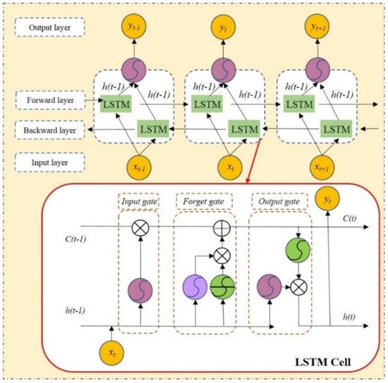
Figure 2.
Deep bidirectional recurrent neural network model.
2.3.2. Encoder–Decoder Structure with Attention Mechanism (EDA-LSTM)
Introducing the encoder–decoder architecture divides the model’s learning process into two stages: encoding and decoding. During the encoding stage, input signals are extracted into an abstract vector, denoted as . In the second stage, this deep vector is mapped to the output signal. This structure enables modeling after a thorough understanding of input semantic features, thereby preserving the continuity of semantics effectively. By incorporating the attention mechanism into the encoder–decoder framework, at each time step, the relevance between the vector and all input time steps in the encoding section is calculated. This allows the model to focus on locally important information and enhance its capacity to capture contextual nuances.
The attention mechanism enables the model, at each time step during the decoding stage, to dynamically select the most relevant portions of the input sequence. It allocates different weights to different parts of the input sequence, to reflect each position’s contribution to the current decoding process. These weights are then normalized to create a context vector, which is combined with the current decoder state to generate the output. This mechanism allows the model to adaptively focus on different parts of the input sequence, enhancing its ability to produce contextually informed outputs.
The context vector can abstract the relationship between the current decoder state and all the encoder states, which is computed as follows:
where and are parameter matrices; and are the transformed vectors of the encoder state and decoder state , where i = 1, 2, …, m − 1, m; α is the relevance measure between and ; is the context vector—here, the subscripts in the formula are in accordance with the Einstein summation convention; represents hidden layer parameters; tanh is the hyperbolic tangent function; and is the bias term.
2.4. One-Dimensional Data Augmentation
Utilizing Generative Adversarial Networks (GANs), we implemented data augmentation for sample data. GANs transform classification problems into generative problems, relying on a loss function that involves both a Generator (G) and a Discriminator (D). This approach is grounded in adversarial learning, where two competing networks capture latent distribution features in sequences, and generate one-dimensional rainfall sequences to augment the dataset, corresponding to driving factors and responses. Figure 3 presents the structure of the GANs.

Figure 3.
Structure of Generative Adversarial Network.
Through competitive adversarial learning, G learns pattern features in the data to generate sequences matching the desired conditions. Specifically, G receives a certain form of input, learns the data distribution from training data, generates target data in the expected form, and feeds the newly generated sequences into D. Simultaneously, D receives both real data and G’s output data, conducts pattern matching on the sequences, and validates the generated sequences using specific criteria. By learning the difference between the distribution of real data and generated data, D enhances its accuracy in checking the target data generated by G. During the training process, G and D are trained alternately, continuously optimizing model parameters through gradient descent.
The loss function employed in GANs is as follows:
where L represents the loss function, denotes the real data distribution, and represents random noise.
2.5. Capture of Water Engineering Scheduling Signals
WEJC regulates river water levels by adjusting the discharge from reservoirs, embankments, or sluice gates in response to the system’s real-time conditions. It involves altering the degree of opening of reservoirs or sluice gates to manage and control water levels and flows in the channels. WEJC consists of two components: the configuration of scheduling schemes and the computation of flow rates for various hydraulic structures. This study constructs two distinct scheduling strategies based on the PBM. Strategy A employs fixed rule-based control (FRC), wherein scheduling curves for water engineering are pre-established before rainfall events. These predetermined curves guide the operation of water engineering systems during intense rainstorms. Conversely, Strategy B adopts dynamic rule-based control (DRC), which adjusts in response to changing conditions within the water system. The scheduling rules are formulated based on the prevailing water system and the inflow rates. DRC adapts to variables in the water system, offering a more optimized real-time control approach. Figure 4 presents the basic process of scheduling.
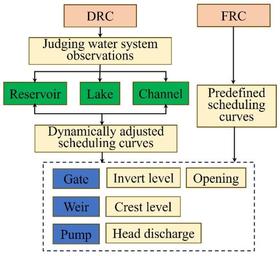
Figure 4.
The basic process of scheduling.
The WEJC system comprises multiple scheduling rules, consisting of scheduling conditions and operations. Scheduling conditions are expressed through conditional expressions. Prior to computing the scheduling rules, multiple scheduling rules are dynamically compiled into executable code using the specified computation mode and program interface. In practice, the gates and weirs serving as outflow control on storage tanks or ponds come in different forms, and we adopt a vertical gate and thin-walled weir. Control of the variable sluice gate is achieved by adjusting the opening height. Flow calculations utilize the thin-plate rectangular weir model when the upstream depth is below the opening height. However, when there is a submerged sluice gate upstream, the flow rate is determined by taking the lesser value between the calculations obtained from the weir equation and the following orifice equations.
The control of variable weirs is achieved by adjusting the weir crest elevation. There are two flow conditions based on the flow over weirs. Free discharge occurs when the downstream depth is below the crest level, and the downstream depth does not affect the upstream discharge. The free outfall discharge (m3/s) is calculated as follows:
The drowned discharge occurs when the downstream depth affects the upstream depth and the discharge, and the downstream depth affects the upstream depth and the discharge. The drowned outfall discharge (m3/s) is calculated as follows:
where is the discharge coefficient; (m/s2) is the acceleration due to gravity; (m) is the width of the weir; and (m) is the upstream depth with respect to the crest.
2.6. Evaluation Metrics
This study adopts the mean absolute error (MAE), the mean squared error (MSE), the mean squared log error (MSLE), and the root mean square error (RMSE) to evaluate the forecast results, and uses a grid map to show the error distribution of the forecast results.
where represents the true value of the sample, is the predicted value of the sample, refers to the index of the sample, is the total number of samples, and ε is a small positive number.
3. Study Area and Materials
3.1. Case Study
Taking the city of Fuzhou’s main urban area as a case study, in recent years, this region has faced the imminent threat of recurrent rainstorm and flood disasters due to rapid urbanization and meteorological factors. The main urban area boasts an extensive network of 42 rivers, with a combined length of 99.3 km and an average river network density exceeding 3 km per square kilometer. The Jin’an River, stretching approximately 6.7 km, serves as the pivotal drainage conduit for the northern sector of the city, seamlessly connecting the upstream mountainous regions with the downstream outer river. During periods of heavy rain and flooding, the Jin’an River shoulders the vital responsibilities of water accumulation, flood regulation, and hydraulic management within the urban area. Consequently, the monitoring and prediction of water levels at key sections of the Jin’an River hold paramount significance for flood prevention efforts in the region [48]. The Jin’an River is an urban landscape river characterized by a stable daily water level ranging from 4 m to 4.5 m, attributed to the presence of water conservation infrastructure.
In the northern mountainous regions of Fuzhou’s main urban zone, four reservoirs and one artificial lake (Guoxi Reservoir, Bayi Reservoir, Douding Reservoir, Jingshan Lake, and Yangting Reservoir) are strategically positioned from west to east. These aquatic reservoirs play a pivotal role within the overall hydrological system. Figure 5 provides a comprehensive overview of the aquatic network in the northern urban area. Furthermore, in this study, two representative water level monitoring stations were selected along the Jin’an River between Qinting Lake and the Guangminggang region. These stations are designated as the Wusi Station (WS) and the Guangminggang Station (GMG). The Bayi Reservoir is located upstream of the study area, and is designed based on the 50-year flood standard. The flood control capacity is 1.11 million m3, with a normal water level of 48.2 m and a flood limit water level of 46.0 m. The spillway is an open-type broad-crested weir with a weir crest elevation of 43.9 m. The Bayi Reservoir plays an effective role in regulating water flow during extreme rainstorms, reducing the risk of flood disasters in the downstream areas [10,48].
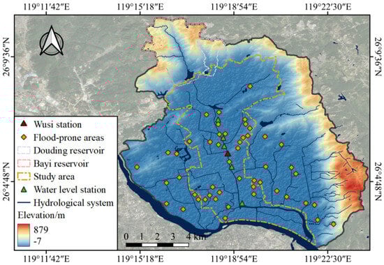
Figure 5.
Study area description.
3.2. Materials
3.2.1. Data Preprocessing
In our previous research [10,48], a model was constructed based on the mechanistic modeling approach described in Section 2.2, and its parameters were calibrated using observed hydrological data (Figure 6). The modeling data usually influence the simulation of hydrodynamic models. Thus, to identify the target points that accurately characterize the hidden feature information, these points must match more closely with the actual research situation.
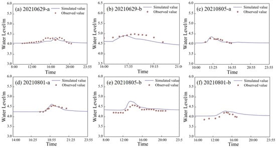
Figure 6.
Calibration and validation periods of PBM: (a) Calibration period (20210629) of junction of Fengban and Jin’an River. (b) Calibration period (20210629) of junction of Qinting Lake and Jin’an River. (c) Calibration period (20210805) of junction of Wusi zone and Jin’an River. (d) Calibration period (20210801) of Jin’an and Dongjiao River. (e) Validation period (20210805) of junction of Qinting Lake and Jin’an River. (f) Validation period (20210801) of junction of Jin’an and Guangming River.
3.2.2. Construction of DDM Dataset
We focused on simulating reservoir operations using data from two selected reservoirs. Specifically, we utilized daily data encompassing inflow, outflow, and storage records to develop a DDM, linking the PBM. We employed five distinct types of rainfalls, including designed rainfall, observed event-based rainfall, typical event-based rainfall, classical rainfall event, and synthesized rainfall data. In the Deep-River model, we synergistically integrated physically based and data-driven approaches. The mechanistic-driven model provided us with a sample dataset, aiding the data-driven model in acquiring additional prior knowledge. To enhance the representativeness of the dataset, we further expanded it using a Generative Adversarial Network (GAN) model, revealing latent rainfall characteristics. Table 1 provides basic information on the five driving rainfall datasets.

Table 1.
Information on different driving rainfall datasets.
Rainfall serves as the crucial dataset driving the model, enabling the generation of datasets encompassing rainfall, reservoir inflow, and dynamic fluctuations in river water levels, using a combination of rainfall data and physically based models. Figure 7 presents four typical rainfall sequences from OER and SER. The datasets from DER, OER, TER, CER, and SER have different time scales and resolutions, and may contain some missing data. Before building the deep learning model, we performed data imputation during the preprocessing stage using Lagrange interpolation, and unified the data from different sources to a consistent time step of 10 min [51].
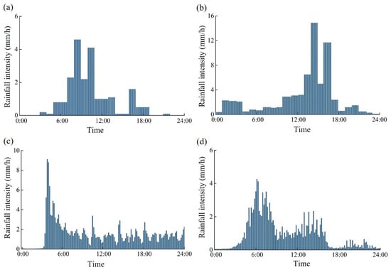
Figure 7.
Typical rainfall sequence: (a) Sample 1 from OER; (b) Sample 2 from OER; (c) Sample 1 from SER; (d) Sample 2 from SER.
Utilizing rainfall data, along with the outflow from Bayi Reservoir and Douding Reservoir and the outlet water level of Qinting Lake, we conducted water level predictions for both the mid-section and downstream section of Jin’an River. The explanatory variables, encompassing rainfall, outflow, and water level, among others, possess varying units of measurement. To ensure a stable and convergent training process, we standardized all feature data across samples first.
3.2.3. Hydraulic Scheduling Modes
This paper presents two scheduling modes: single-point scheduling (SPS) and multi-point joint scheduling (MPS). SPS refers to the regulation of individual hydraulic projects at a single location, which, in practice, can be controlled by a system composed of multiple basic hydraulic units. MPS refers to the coordinated scheduling of hydraulic systems at different locations. The combined scheduling of hydraulic projects at multiple spatial locations is not equivalent to a linear superposition of individual location-based hydraulic scheduling. Based on the inflow from the upstream catchment, and river and lake safety water levels, as well as empirical scheduling rules, joint scheduling rules for the Bayi reservoir, Qinting lake, and Jingdian lake were designed. The real-time control strategy is outlined in Table 2. Additionally, we adopted a non-scheduling control (NSC) as the baseline. This baseline scheme does not actively regulate hydraulic engineering facilities, but instead relies on natural hydrological processes to manage water flow.
Table 2.
Model structure of BSA--LSTM.
Individual rules were established for three water projects to adapt to specific complex water system conditions: (1) The Bayi reservoir plays a crucial role in the flood control system of the study area. Specifically, in anticipation of sudden heavy rainfall, the pre-gate water level is lowered, and each orifice of the middle orifice gate is opened by 0.3 m, starting from an initial elevation of 44.0 m. The outflow from the reservoir is controlled by four adjustable gates and one non-adjustable weir, with the gate openings dynamically adjusted based on the reservoir’s water level. Each gate has a base elevation of 44.0 m, a width of 6.5 m, a discharge coefficient of 0.72, and a normal opening height of 4.8 m. (2) Qinting lake receives runoff from the surrounding urban areas and upstream river inflow, with outflow controlled by five adjustable weirs. The weir crest has a height of 4.5 m and a width of 8 m, with a discharge coefficient of 0.85. During real-time control, the outflow is adjusted by changing the weir crest elevation. (3) Jingdian lake is equipped with two inlet gates and one outlet gate. The inlet gates (#1 and #2) are used to provide storage functionality for Jingdian lake and collect runoff from the upstream watershed under specific conditions. When there is a decreasing trend in the water levels of Qinting lake or the Jiefang river, the outlet gate (#3) is opened, with the maximum discharge controlled to be within 20 m3/s.
4. Results and Discussion
4.1. Model Performance of Deep-River
Using the BSA-LSTM architecture, as presented in Table 2, we conducted water level forecasting for both stations WS and GMG along the Jin’an River. The BSA-LSTM model configuration consists of one input layer, two LSTM layers, one self-attention layer, and one fully connected layer. The input layer has a dimension of 145 × 4, with each LSTM layer containing 50 output units, while the self-attention layer is equipped with 50 output units, and the fully connected layer comprises 145 output units. The model training leverages the Adam optimization algorithm for backpropagation, with a learning rate of 0.001. We opted for a batch size of 30 for each round of model training, taking into account two pivotal considerations:
Employing a batch size allows for efficient loading of data into memory, enabling parallel processing using GPU resources, thereby circumventing the resource-intensive nature of serial computation. Choosing an appropriate batch size (BS) is crucial for ensuring the convergence of gradient-based optimization algorithms. A batch size that is too small may introduce fluctuations in model accuracy, whereas an excessively large BS may lead to the model becoming trapped in local optima. Therefore, the selection of a BS of 30 strikes a harmonious balance between computational efficiency and effective model convergence.
The variation in model errors for the WS station and GMG station water level prediction model during the training and validation periods is illustrated in Figure 8. After 500 training iterations employing the gradient descent algorithm, the model’s metrics exhibited a decreasing trend. At this stage, the model reached a reasonable level of convergence. While certain metrics, such as RMSE, might have still had potential for further reduction on the training dataset, they had already stabilized on the validation dataset. It is worth noting that excessively high metrics on the training dataset could indicate overfitting. In the test dataset, the model achieved the following performance metrics: the MSE was 0.001, the MAE was 0.012, the MSLE was 0.0007, and the RMSE was 0.033. Employing the gradient descent algorithm over 500 training iterations, the model’s metrics exhibited a fluctuating descent pattern. Throughout the iterative process, the reduction in loss for both the validation and training phases closely corresponded. In the test dataset, the model achieved the following performance metrics: the MSE was 0.001, the MAE was 0.014, the MSLE was 0.0006, and the RMSE was 0.031.
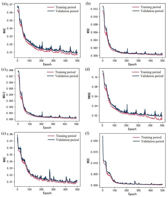
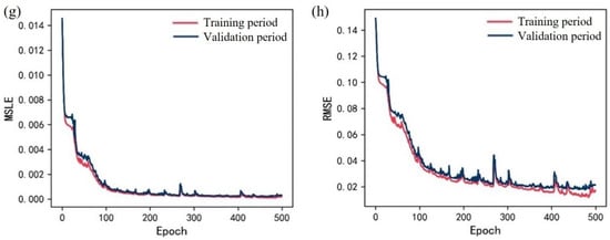
Figure 8.
Error change during training period and validation period: (a) MAE of WS; (b) MSE of WS; (c) MSLE of WS; (d) RMSE of WS; (e) MAE of GMG; (f) MSE of GMG; (g) MSLE of GMG; (h) RMSE of GMG.
4.2. Uncertainty Analysis of Model Hyperparameters
Models inherently possess a degree of uncertainty, arising from various sources, such as the model’s intrinsic components (including model parameters, structure, and algorithms), external data, and observational errors, among others [49,50]. Based on the model developed in Section 4.1, we conducted an analysis of the sensitivity of the model’s performance to key model parameters.
4.2.1. Hidden Layer Number
The hidden layer number (HLN) indicates the quantity of nodes employed to represent the hidden state within the model. Specifically, within the model, the current state is conveyed to the previous time step through forward connections. The parameter HLN is employed to signify the quantity of nodes used for retaining and storing past states. Figure 9 graphically illustrates the impact of the parameter HLN on four evaluation metrics (MAE, MSE, MSLE, and RMSE) when varied across a range from 10 to 150.

Figure 9.
Response of model performance to HLN: (a) MAE; (b) MSE; (c) MSLE; (d) RMSE.
Observations reveal that alterations in all four metrics exhibit a consistent pattern. Overall, the model’s performance optimizes at a local maximum when the HLN is set to either 80 or 130. The model’s performance demonstrates a rapid ascent as the HLN escalates from 10 to 80. Nevertheless, when the HLN is fixed at 110, the model’s performance experiences a substantial dip. Furthermore, when the HLN exceeds 120, the model’s performance registers a swift recovery. The graph plainly illustrates that a small number of hidden layers or a setting of 110 adversely impacts model performance. This implies that an insufficient number of hidden layers results in incomplete retention or retrieval of information from the time steps preceding the current one, consequently causing a decrease in model performance. Nevertheless, a mere increase in the HLN does not consistently enhance simulation performance, and may even induce localized fluctuations in performance.
4.2.2. Batch Size
The batch size (BS) parameter determines how many samples are processed in parallel during each training round, and is closely tied to the dataset’s size. Selecting a value of BS that is too large can increase the risk of getting stuck in local optima during the backpropagation process. Conversely, if the BS is too small, it introduces greater randomness in each training round, making it challenging for the gradient descent algorithm to effectively update model weights in the steepest direction, which can hinder convergence towards the optimal solution. Considering the dataset’s size, we conducted experiments to assess how the model’s performance reacts to varying BSs, ranging from 5 to 60.
Figure 10 provides an overview of the model’s performance metrics (MAE, MSE, MSLE, RMSE) as the BS changes on the testing dataset. These metrics exhibit consistent trends across the different BS values. Notably, when the parameter BS is set to 45, all four metrics reach their maximum values, indicating relatively poor model performance at this point. In practice, as the BS increases, there is an overall trend of diminishing model performance, although distinct fluctuations in model performance are observed within specific ranges. In general, a smaller BS parameter, typically below 25, tends to yield better model performance.
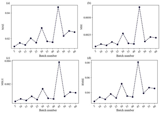
Figure 10.
Response of model performance to BS: (a) MAE; (b) MSE; (c) MSLE; (d) RMSE.
4.2.3. Learning Rate
The weights and bias of the network are updated based on the chain rule of loss differentiation under a given learning rate (LR) parameter. When the LR is too large, the weights and bias update rapidly, but the model may struggle to converge to the global optimum. Conversely, with an excessively small LR, the model learns slowly, and is susceptible to getting trapped in local optima [52].
Figure 11 illustrates the changes in the model’s four evaluation metrics (MAE, MSE, MSLE, RMSE) as the LR varies between 0.001 and 0.18. It is observed that the MAE, MSE, and RMSE exhibit consistent trends, while the MSLE shows slight differences when the LR exceeds 0.14. The results indicate that when the LR is less than 0.1, the four evaluation metrics are relatively low, indicating better model performance. Furthermore, within this range of LR values, the model performance remains relatively stable. However, when the LR exceeds 0.15, significant oscillations in model performance become apparent.
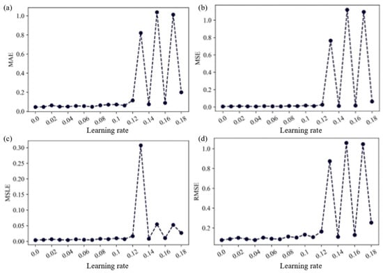
Figure 11.
Response of model performance to LR: (a) MAE; (b) MSE; (c) MSLE; (d) RMSE.
4.3. Uncertainty Analysis of Model Structures
4.3.1. Comparison of Model Structures
The Deep-River framework introduces uncertainty into the model performance, due to variations in model structures. This study compares five distinct models within the Deep-River framework: (1) Bi-LSTM (B-LSTM); (2) Bi-Stack-LSTM (BS-LSTM); (3) Attention-LSTM (A-LSTM); (4) ED-LSTM; and (5) ED-Attention-LSTM (EDA-LSTM). Detailed network architectures and parameter counts for these five models are provided in Table 3. The B-LSTM model exhibits an output dimension of 145 × 1, and necessitates separate model configurations for simulating the water levels at station WS and station GMG. BS-LSTM enhances the B-LSTM model by introducing two bidirectional LSTM layers, increasing the model complexity and enabling the extraction of features abstracted by shallow networks using deeper networks. A-LSTM incorporates self-attention mechanisms into the model. ED-LSTM adopts an encoder–decoder architecture, thoroughly extracting input features and dynamically forecasting the water level at the target station. EDA-LSTM builds upon the ED-LSTM model by introducing attention mechanisms, calculating the relevance of input features to the decoder at each time step, thereby reinforcing the integration of locally relevant information during the decoding process.
Table 3.
Comparison of different model architectures.
4.3.2. Evaluation of Model Performances
The selection of hyperparameters and solvers directly impacts the model performance. To ensure a fair comparison among these five different architectural models, specific parameters were standardized. The HLN was set to 30, the activation function was chosen as Adam, and the LR was set to 0.001. Prior to model training, the dataset underwent random partitioning into training, validation, and test sets in a predefined ratio (30% for testing, 70% for training, and 30% for validation). Random dataset splits can introduce variability in results. To mitigate the influence of this randomness on metric evaluation, each scenario was independently tested 10 times. The average values from these ten trials were computed as the evaluation results. All four metrics were computed on the test set, which provides a better gauge of the model’s generalization ability compared to the training and validation sets.
Table 4 presents the performance evaluation metrics for water level simulation at station WS, and Table 5 displays the evaluation metrics for water level simulation at station GMG. It is evident that BS-LSTM performs the best, followed by B-LSTM and A-LSTM, with ED-LSTM and EDA-LSTM demonstrating relatively weak performance. In fact, all models achieve reasonably good simulation results. However, the superior performance of B-LSTM, BS-LSTM, and A-LSTM can be attributed, in part, to the fact that these three models have only one-dimensional output vectors, while the latter two models have two-dimensional output vectors. The first three models require separate modeling for the two stations, preventing weight parameter sharing between them, and making their learning of input features dependent on input time steps. In contrast, the models based on the encoder–decoder architecture have stronger capabilities in semantic understanding and output. Furthermore, when comparing the results of the first three models, it becomes evident that there is an upper limit to model complexity, and increasing the number of network layers can enhance model performance to a certain extent. In practice, it is advisable to choose the specific model architecture based on the dataset characteristics.
Table 4.
Simulation results of model at station WS.
Table 5.
Simulation results of model at station GMG.
4.4. Capturing Flooding Response for Regional Controls
4.4.1. Joint Scheduling Analysis Based on DRC
Based on DRC, we compared the downstream river water levels under three different scheduling control drivers: SPS, MPS, and SCS (Figure 12). In section a, the water levels were 7.760 m, 8.018 m, and 8.393 m for SPS, MPS, and SCS, respectively. The maximum water level under MPS was 0.633 m higher than that under SCS. In section b, the water levels were 5.993 m, 6.007 m, and 6.223 m, with a peak water level difference of 0.23 m between MPS and SCS. Regarding flow rates, section a exhibited discharge values of 210.339 m3/s, 239.551 m3/s, and 274.014 m3/s for SPS, MPS, and SCS, respectively. Similarly, in section b, the flow rates were 291.836 m3/s, 303.661 m3/s, and 353.861 m3/s. By comparing the simulation results across different scenarios, it is evident that the upstream river responds more significantly to MPS, while SPS demonstrates an intermediate effect between MPS and SCS.
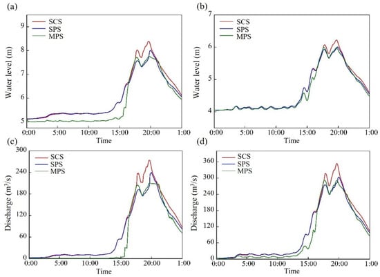
Figure 12.
Water levels and discharges under three scheduling modes: (a) water level in section a; (b) water level in section b; (c) discharge in section a; (d) discharge in section b.
4.4.2. Regional Control Signals Capturing Based on FRC
The parameter space of flood systems typically has a high dimensionality, and the optimal parameters found within the solution space are influenced by the driving conditions. We captured the scheduling information under designed storm events based on fixed rule-based control (FRC) and three different rainfall peak coefficients (0.2, 0.398, and 0.8). With the introduction of joint scheduling measures, the flood peak regulation effect on river water levels became evident. The original single-peak water level curve transformed into a double-peak pattern (Figure 13). Before the flood arrived, the sluice gates were opened to release water and create storage capacity, ensuring maximum retention when the flood peak occurred. Specifically, for Storage Bayi, the initial opening height of five sluice gates was set to 8 m, and three hours after the rainfall peak, the gate height was adjusted to 4.5 m. Meanwhile, for Storage Qinting, the crest height of the downstream weir was initially set to 3 m, and was later adjusted to 5 m three hours after the rainfall peak. Under a 100-year storm return period, the following relationships hold for the MPS and SCS modes at a given time:
where represents the water level under SCS; t is time; and is a small value. As shown in Figure 13, the water level at the monitoring site reaches its peak around 10:10, with a maximum value of approximately 6.14 m under SCS. When MPS is introduced, the peak water level decreases to around 5.84 m. During the subsequent period, the water level remains relatively low. The retained floodwater forms a local maximum at approximately 16:30, but this peak is significantly lower than the previous one.
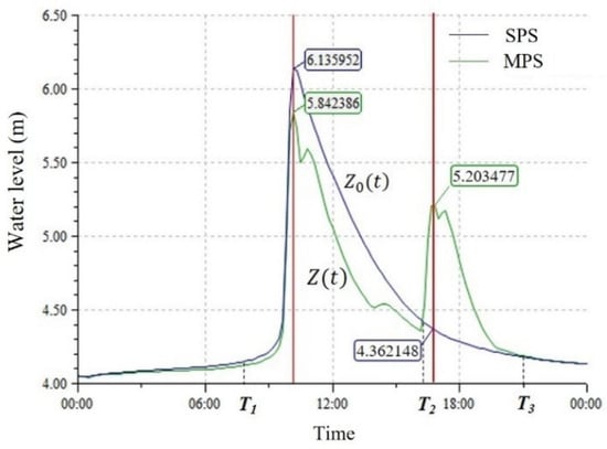
Figure 13.
Dispatching condition analysis.
Based on the A-LSTM architecture, a dual-layer temporal feature extraction module was introduced. The dataset was split into 60% for training, 20% for validation, and 20% for testing. The model converged rapidly within the first 50 epochs, after which changes became minimal, indicating that the evaluation metrics had stabilized. Since all four metrics approached zero, the model could be considered fully converged. When evaluated on the test set, the model achieved the following performance metrics: an MAE of 0.0039, an MSE of 6.03 × 10⁻⁵, an MSLE of 3.79 × 10⁻⁵, and an RMSE of 0.0078.
Figure 14 presents the simulation results after incorporating scheduling information, showing Sample 13 and Sample 32 from the test set. The simulated values for Sample 13 closely match the observed values, with a maximum simulated water level of 5.28 m and a maximum observed water level of 5.20 m. The largest deviation occurs between 10:30 and 13:00, while the two curves remain largely consistent at other times. Similarly, for Sample 32, the simulated values align well with the observations, with a maximum simulated water level of 5.15 m and a maximum observed water level of 5.19 m. The most significant deviation is observed between 11:00 and 16:30, while the water levels remain consistent during other periods. After encoding the scheduling information, the water level process exhibits a “double-peak” pattern, with the first peak significantly lower compared to the peak under non-scheduling conditions. The A-LSTM model effectively captures the overall trend of flood wave propagation, but its ability to extract features of local variations with large fluctuations is relatively weaker. This limitation is partly due to the scale of the dataset and the insufficiency of information. With the introduction of scheduling rules, external influences such as water engineering regulation cause localized fluctuations at the WS station. The limited number of data samples and training epochs restrict the model’s ability to fully learn and generalize local response characteristics over specific time intervals.
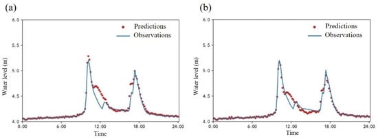
Figure 14.
Simulation results of introducing scheduling information: (a) Sample 13; (b) Sample 32.
4.5. Discussion
4.5.1. Advantages of Integrating Physically Based Models and Data-Driven Models
The PBM provides a reliable explanation for hydrodynamic processes and flood behavior based on physical laws. Its advantage lies in the ability to quantify and analyze each sub-process within the complex flood process [53]. However, such models, which rely on hydrological and hydrodynamic mechanisms, require high-precision terrain and underlying surface data, resulting in high computational costs, especially in the field of two-dimensional inundation processes involving high-resolution simulations [10]. Despite being based on physical mechanisms, the solution process is still a significant simplification of real-world problems, which makes these models less effective and reliable when applied to urban-scale studies, where human activities have a profound impact, compared to small-scale studies [15,16]. In complex urban systems, uncertainty in monitoring, data, and other aspects makes it difficult for hydrological and hydrodynamic models to capture the intricate nonlinear interactions in the system, particularly when fine-scale terrain, infrastructure, and human activities are involved [54]. The DDM performs efficiently in modeling complex relationships and patterns in larger datasets. It can identify subtle interactions that may be difficult to manually encode, making it a powerful tool in flood prediction. However, purely data-driven models often lack physical interpretability and depend heavily on the availability and accuracy of the dataset. This may limit their reliability, especially when applied to scenarios with sparse or unrepresentative data, particularly in extreme conditions [55].
The hybrid method proposed in this paper combines the interpretability of the PBM with the pattern recognition capabilities of the DDM. The PBM provides simulation datasets for pluvial flooding, which greatly supplements the sample features required for deep learning. In urban water management, the focus is often not on the entire process of feature evolution, but rather on specific features at specific locations. This hybrid simulation method also offers a means for performing end-to-end nonlinear simulations, based on an encoder–decoder architecture and attention mechanisms, creating a simulation framework with strong generalization ability. Moreover, combining these two methods can significantly improve computational efficiency during the application phase. Although large sample sizes may result in considerable computational resource consumption during the deep learning model training process, this training is typically separate from the application phase. Once training is completed, meaning the loss function has been iteratively satisfied, the trained model can be used to predict unknown scenarios. This deep learning model, with good scalability, has minimal time consumption during the prediction process, making it suitable for real-time flood forecasting and decision-making in urban environments.
This study provides urban planners with a robust tool for improving flood risk assessments and management. The inclusion of scheduling control signals allows planners to optimize flood control measures, such as drainage and pumps. Additionally, the framework can help to identify vulnerable areas and design resilient infrastructure, while its predictive capabilities support real-time flood forecasting and better resource allocation.
4.5.2. Limitations and Future Work
This study proposes a framework that combines physically based models with deep learning approaches. To supplement and enhance the dataset, we use multiple synthetic data for data augmentation, increasing the diversity and quantity of training samples, which improves the model’s generalization capability. The framework considers the impact of scheduling control signals on flood dynamics and incorporates them into the model. The inclusion of scheduling information results in a “double-peak” pattern in the water level process, indicating that scheduling has a significant influence on the temporal evolution of floods. However, there are certain limitations to this study. The quality of generated data means that they may not fully replace real observational data, and due to the limited availability of measured data, the model needs further training with more diverse data samples to better match the model complexity with the training data. While scheduling control signals show some influence in the simulation, the current model’s scheduling data are based on specific scenarios, and there is a lack of in-depth research on diverse scheduling strategies and complex real-world scheduling mechanisms. Accurately capturing scheduling control signals in different cities and conditions remains an unresolved issue. Although the current approach performs well in flood simulation for specific regions or cities, its generalizability needs further validation. Moreover, different cities have varying geographical features, climate conditions, and urban layouts, which may require further adjustments and optimization of the model based on specific circumstances.
Future research will introduce more complex scheduling strategies based on richer sample data and greater feature diversity to enhance the model’s adaptability and practical utility. Additionally, future studies could expand the applicability of this framework to explore flood simulation in different climatic and urban environments, while integrating remote sensing monitoring and big data analysis to further improve the intelligence and accuracy of flood early warning systems.
5. Conclusions
We have developed an analytical framework known as Deep-River, and the framework continues to employ an object-oriented programming approach, enabling an “end-to-end” analysis of the model. The framework accomplishes four primary functions:
- (1)
- The Deep-River framework was developed based on the evolution characteristics of urban river flooding. The framework integrates multiple models, including B-LSTM, BS-LSTM, A-LSTM, ED-LSTM, and EDA-LSTM. The model performances at stations WS and GMG demonstrate a good fit of the Deep-River framework.
- (2)
- Model uncertainty stems from the parameters and structure. Optimal performance occurs at 80 or 130 hidden layers, with too few layers causing information loss, and too many leading to fluctuations. A batch size below 25 yields better results, while learning rates above 0.15 cause instability. BS-LSTM performs best, followed by B-LSTM and A-LSTM, due to their 1D output vectors, unlike ED-LSTM and EDA-LSTM, which allow weight sharing across stations. Increasing network depth within limits improves performance, with ED-LSTM and EDA-LSTM excelling in multi-station water level prediction.
- (3)
- Based on the A-LSTM architecture, a self-attention mechanism was introduced to capture the evolution characteristics of river flooding under scheduling influences. The results indicate that the dual-layer self-attention LSTM model exhibits strong adaptability. With scheduling information encoding, the simulated water level process shows a “double-peak” pattern, with the first peak significantly lower than that under non-scheduling conditions. The model effectively extracts global flood wave evolution trends, though its ability to capture local variations with large fluctuations is relatively weak.
The Deep-River framework offers practical support for urban pluvial river flooding forecasting, flood management, and urban planning.
Author Contributions
Conceptualization, C.Y., Z.X. and W.L.; Methodology, C.Y.; Software, X.S.; Validation, Z.X. and X.S.; Formal analysis, W.L. and X.L.; Investigation, Z.X., W.L., X.L. and X.S.; Resources, W.L. and X.L.; Data curation, W.L.; Writing—original draft, C.Y.; Writing—review & editing, C.Y., Z.X. and X.S.; Visualization, C.Y.; Supervision, Z.X. and X.L.; Project administration, C.Y.; Funding acquisition, C.Y. All authors have read and agreed to the published version of the manuscript.
Funding
This study was supported by the National Natural Science Foundation of China (52409005), the China Postdoctoral Science Foundation (2024M750224), and the National Natural Science Foundation of China (52239003).
Institutional Review Board Statement
Not applicable.
Informed Consent Statement
Not applicable.
Data Availability Statement
The original contributions presented in the study are included in the article, further inquiries can be directed to the corresponding author.
Conflicts of Interest
The authors declare no conflict of interest.
References
- Rubinato, M.; Nichols, A.; Peng, Y.; Zhang, J.M.; Lashford, C.; Cai, Y.P.; Lin, P.Z.; Tait, S. Urban and river flooding: Comparison of flood risk management approaches in the UK and China and an assessment of future knowledge needs. Water Sci. Eng. 2019, 12, 274–283. [Google Scholar] [CrossRef]
- Qi, M.; Huang, H.; Liu, L.; Chen, X. Spatial heterogeneity of controlling factors’ impact on urban pluvial flooding in Cincinnati, US. Appl. Geogr. 2020, 125, 102362. [Google Scholar] [CrossRef]
- Balistrocchi, M.; Grossi, G. Predicting the impact of climate change on urban drainage systems in northwestern Italy by a copula-based approach. J. Hydrol. Reg. Stud. 2020, 28, 100670. [Google Scholar] [CrossRef]
- Dash, P.; Punia, M. Governance and disaster: Analysis of land use policy with reference to Uttarakhand flood 2013, India. Int. J. Disaster Risk Reduct. 2019, 36, 101090. [Google Scholar] [CrossRef]
- Xu, T.; Li, K.; Engel, B.A.; Jia, H.; Leng, L.; Sun, Z.; Shaw, L.Y. Optimal adaptation pathway for sustainable low impact development planning under deep uncertainty of climate change: A greedy strategy. J. Environ. Manag. 2019, 248, 109280. [Google Scholar] [CrossRef]
- Kind, J.; Wouter Botzen, W.J.; Aerts, J.C. Accounting for risk aversion, income distribution and social welfare in cost-benefit analysis for flood risk management. Wiley Interdiscip. Rev. Clim. Change 2017, 8, e446. [Google Scholar] [CrossRef]
- Yin, J.; Yu, D.; Yin, Z.; Liu, M.; He, Q. Evaluating the impact and risk of pluvial flash flood on intra-urban road network: A case study in the city center of Shanghai, China. J. Hydrol. 2016, 537, 138–145. [Google Scholar] [CrossRef]
- Meng, Z.; Yao, D. Damage survey, radar, and environment analyses on the first-ever documented tornado in Beijing during the heavy rainfall event of 21 July 2012. Weather Forecast. 2014, 29, 702–724. [Google Scholar] [CrossRef]
- Huang, X.; Liu, G.; Liu, S.; Fan, Y.; Ma, J.; Fan, Z. Study on numerical simulation method of extreme rain flood risk in plain river network cities. China Flood Drought Manag. 2023, 33, 21–27,33. (In Chinese) [Google Scholar]
- Ye, C.; Xu, Z.; Lei, X.; Liao, W.; Ding, X.; Liang, Y. Assessment of urban flood risk based on data-driven models: A case study in Fuzhou City, China. Int. J. Disaster Risk Reduct. 2022, 82, 103318. [Google Scholar] [CrossRef]
- Berndtsson, R.; Becker, P.; Persson, A.; Aspegren, H.; Haghighatafshar, S.; Jönsson, K.; Larsson, R.; Mobini, S.; Mottaghi, M.; Nilsson, J.; et al. Drivers of changing urban flood risk: A framework for action. J. Environ. Manag. 2019, 240, 47–56. [Google Scholar] [CrossRef] [PubMed]
- Miller, J.D.; Hutchins, M. The impacts of urbanisation and climate change on urban flooding and urban water quality: A review of the evidence concerning the United Kingdom. J. Hydrol. Reg. Stud. 2017, 12, 345–362. [Google Scholar] [CrossRef]
- Qin, D.; Lu, C.; Liu, J.; Wang, H.; Wang, J.; Li, H.; Chu, J.; Chen, G. Theoretical framework of dualistic nature–social water cycle. Chin. Sci. Bull. 2014, 59, 810–820. [Google Scholar] [CrossRef]
- Zhang, S.; Fan, W.; Yi, Y.; Zhao, Y.; Liu, J. Evaluation method for regional water cycle health based on nature-society water cycle theory. J. Hydrol. 2017, 551, 352–364. [Google Scholar] [CrossRef]
- Liu, J.; Shao, W.; Xiang, C.; Mei, C.; Li, Z. Uncertainties of urban flood modeling: Influence of parameters for different underlying surfaces. Environ. Res. 2020, 182, 108929. [Google Scholar] [CrossRef]
- Ye, C.; Liao, W.; Xu, Z.; Li, X.; Shu, X. An enhanced framework for simulating urban pluvial flooding: Integrating nested watersheds and urban areas with spatial heterogeneity. J. Hydrol. 2025, 654, 132875. [Google Scholar] [CrossRef]
- Chen, Y.; Wang, C.; Yang, Q.; Lei, X.; Wang, H.; Jiang, S.; Wang, Z. Model predictive control and rainfall Uncertainties: Performance and risk analysis for drainage systems. J. Hydrol. 2024, 630, 130779. [Google Scholar] [CrossRef]
- Cao, W.; Zhou, Y.; Güneralp, B.; Li, X.; Zhao, K.; Zhang, H. Increasing global urban exposure to flooding: An analysis of long-term annual dynamics. Sci. Total Environ. 2022, 817, 153012. [Google Scholar] [CrossRef]
- Lin, T.; Liu, X.; Song, J.; Zhang, G.; Jia, Y.; Tu, Z.; Zheng, Z.; Liu, C. Urban waterlogging risk assessment based on internet open data: A case study in China. Habitat Int. 2018, 71, 88–96. [Google Scholar] [CrossRef]
- Konami, T.; Koga, H.; Kawatsura, A. Role of pre-disaster discussions on preparedness on consensus-making of integrated flood management (IFM) after a flood disaster, based on a case in the Abukuma River Basin, Fukushima, Japan. Int. J. Disaster Risk Reduct. 2021, 53, 102012. [Google Scholar] [CrossRef]
- Qi, W.; Ma, C.; Xu, H.; Chen, Z.; Zhao, K.; Han, H. A review on applications of urban flood models in flood mitigation strategies. Nat. Hazards 2021, 108, 31–62. [Google Scholar] [CrossRef]
- Salvadore, E.; Bronders, J.; Batelaan, O. Hydrological modelling of urbanized catchments: A review and future directions. J. Hydrol. 2015, 529, 62–81. [Google Scholar] [CrossRef]
- Mark, O.; Weesakul, S.; Apirumanekul, C.; Aroonnet, S.B.; Djordjević, S. Potential and limitations of 1D modelling of urban flooding. J. Hydrol. 2004, 299, 284–299. [Google Scholar] [CrossRef]
- Ferraro, D.; Costabile, P.; Costanzo, C.; Petaccia, G.; Macchione, F. A spectral analysis approach for the a priori generation of computational grids in the 2-D hydrodynamic-based runoff simulations at a basin scale. J. Hydrol. 2020, 582, 124508. [Google Scholar] [CrossRef]
- Hou, J.; Zhou, N.; Chen, G.; Huang, M.; Bai, G. Rapid forecasting of urban flood inundation using multiple machine learning models. Nat. Hazards 2021, 108, 2335–2356. [Google Scholar] [CrossRef]
- Eini, M.; Kaboli, H.S.; Rashidian, M.; Hedayat, H. Hazard and vulnerability in urban flood risk mapping: Machine learning techniques and considering the role of urban districts. Int. J. Disaster Risk Reduct. 2020, 50, 101687. [Google Scholar] [CrossRef]
- Zhao, G.; Pang, B.; Xu, Z.; Peng, D.; Xu, L. Assessment of urban flood susceptibility using semi-supervised machine learning model. Sci. Total Environ. 2019, 659, 940–949. [Google Scholar] [CrossRef]
- Situ, Z.; Zhong, Q.; Zhang, J.; Teng, S.; Ge, X.; Zhou, Q.; Zhao, Z. Attention-based deep learning framework for urban flood damage and risk assessment with improved flood prediction and land use segmentation. Int. J. Disaster Risk Reduct. 2025, 116, 105165. [Google Scholar] [CrossRef]
- Chen, C.; Jiang, J.; Liao, Z.; Zhou, Y.; Wang, H.; Pei, Q. A short-term flood prediction based on spatial deep learning network: A case study for Xi County, China. J. Hydrol. 2020, 607, 127535. [Google Scholar] [CrossRef]
- Zhu, S.; Wei, J.; Zhang, H.; Xu, Y.; Qin, H. Spatiotemporal deep learning rainfall-runoff forecasting combined with remote sensing precipitation products in large scale basins. J. Hydrol. 2023, 616, 128727. [Google Scholar] [CrossRef]
- Moon, H.; Yoon, S.; Moon, Y. Urban flood forecasting using a hybrid modeling approach based on a deep learning technique. J. Hydroinformatics 2023, 25, 593–610. [Google Scholar] [CrossRef]
- Chen, Z.; Lin, H.; Shen, G. TreeLSTM: A spatiotemporal machine learning model for rainfall-runoff estimation. J. Hydrol. Reg. Stud. 2023, 48, 101474. [Google Scholar] [CrossRef]
- Kim, H.I.; Han, K.Y. Urban flood prediction using deep neural network with data augmentation. Water 2020, 12, 899. [Google Scholar] [CrossRef]
- Guo, Z.; Leitao, J.P.; Simões, N.E.; Moosavi, V. Data-driven flood emulation: Speeding up urban flood predictions by deep convolutional neural networks. J. Flood Risk Manag. 2021, 14, e12684. [Google Scholar] [CrossRef]
- Darabi, H.; Choubin, B.; Rahmati, O.; Haghighi, A.T.; Pradhan, B.; Kløve, B. Urban flood risk mapping using the GARP and QUEST models: A comparative study of machine learning techniques. J. Hydrol. 2019, 569, 142–154. [Google Scholar] [CrossRef]
- Lin, L.; Tang, C.; Liang, Q.; Wu, Z.; Wang, X.; Zhao, S. Rapid urban flood risk mapping for data-scarce environments using social sensing and region-stable deep neural network. J. Hydrol. 2023, 617, 128758. [Google Scholar] [CrossRef]
- Mohamadiazar, N.; Ebrahimian, A.; Hosseiny, H. Integrating deep learning, satellite image processing, and spatial-temporal analysis for urban flood prediction. J. Hydrol. 2024, 639, 131508. [Google Scholar] [CrossRef]
- Feng, B.; Wang, J.; Zhang, Y.; Hall, B.; Zeng, C. Urban flood hazard mapping using a hydraulic–GIS combined model. Nat. Hazards 2020, 100, 1089–1104. [Google Scholar] [CrossRef]
- Wu, Z.; Ma, B.; Wang, H.; Hu, C.; Lv, H.; Zhang, X. Identification of sensitive parameters of urban flood model based on artificial neural network. Water Resour. Manag. 2021, 35, 2115–2128. [Google Scholar] [CrossRef]
- Berkhahn, S.; Fuchs, L.; Neuweiler, I. An ensemble neural network model for real-time prediction of urban floods. J. Hydrol. 2019, 575, 743–754. [Google Scholar] [CrossRef]
- Bermúdez, M.; Cea, L.; Puertas, J. A rapid flood inundation model for hazard mapping based on least squares support vector machine regression. J. Flood Risk Manag. 2019, 12, e12522. [Google Scholar] [CrossRef]
- Yan, J.; Jin, J.; Chen, F.; Yu, G.; Yin, H.; Wang, W. Urban flash flood forecast using support vector machine and numerical simulation. J. Hydroinformatics 2018, 20, 221–231. [Google Scholar] [CrossRef]
- Sadler, J.M.; Goodall, J.L.; Morsy, M.M.; Spencer, K. Modeling urban coastal flood severity from crowd-sourced flood reports using Poisson regression and Random Forest. J. Hydrol. 2018, 559, 43–55. [Google Scholar] [CrossRef]
- Lin, J.; He, X.; Lu, S.; Liu, D.; He, P. Investigating the influence of three-dimensional building configuration on urban pluvial flooding using random forest algorithm. Environ. Res. 2021, 196, 110438. [Google Scholar] [CrossRef]
- Wu, Z.; Zhou, Y.; Wang, H.; Jiang, Z. Depth prediction of urban flood under different rainfall return periods based on deep learning and data warehouse. Sci. Total Environ. 2020, 716, 137077. [Google Scholar] [CrossRef]
- Yang, F.; Ding, W.; Zhao, J.; Song, L.; Yang, D.; Li, X. Rapid urban flood inundation forecasting using a physics-informed deep learning approach. J. Hydrol. 2024, 643, 131998. [Google Scholar] [CrossRef]
- Le, X.H.; Nguyen, D.H.; Jung, S.; Yeon, M.; Lee, G. Comparison of deep learning techniques for river streamflow forecasting. IEEE Access 2021, 9, 71805–71820. [Google Scholar] [CrossRef]
- Ye, C.; Xu, Z.; Lei, X.; Zhang, R.; Chu, Q.; Li, P.; Ban, C. Assessment of the impact of urban water system scheduling on urban flooding by using coupled hydrological and hydrodynamic model in Fuzhou City, China. J. Environ. Manag. 2022, 321, 115935. [Google Scholar] [CrossRef]
- Gupta, A.; Govindaraju, R.S. Propagation of structural uncertainty in watershed hydrologic models. J. Hydrol. 2019, 575, 66–81. [Google Scholar] [CrossRef]
- Knoben, W.J.; Freer, J.E.; Peel, M.C.; Fowler, K.J.A.; Woods, R.A. A brief analysis of conceptual model structure uncertainty using 36 models and 559 catchments. Water Resour. Res. 2020, 56, e2019WR025975. [Google Scholar] [CrossRef]
- Chenlei, Y.E.; Zongxue, X.U.; Weihong, L.I.A.O.; Xinyi, S.H.U.; Ruting, L.I.A.O. Urban pluvial flooding process: Semi-distributed tank model and river flood simulation. J. Beijing Norm. Univ. Nat. Sci. 2024, 60, 667–680. [Google Scholar]
- Yang, S.; Yang, D.; Chen, J.; Zhao, B. Real-time reservoir operation using recurrent neural networks and inflow forecast from a distributed hydrological model. J. Hydrol. 2019, 579, 124229. [Google Scholar] [CrossRef]
- Liang, Y.; Liao, W.; Zhang, Z.; Li, H.; Wang, H. Using a multiphysics coupling-oriented flood modelling approach to assess urban flooding under various regulation scenarios combined with rainstorms and tidal effects. J. Hydrol. 2024, 645, 132189. [Google Scholar] [CrossRef]
- Huang, H.; Lei, X.; Liao, W.; Liu, D.; Wang, H. A hydrodynamic-machine learning coupled (HMC) model of real-time urban flood in a seasonal river basin using mechanism-assisted temporal cross-correlation (MTC) for space decoupling. J. Hydrol. 2023, 624, 129826. [Google Scholar] [CrossRef]
- Rasool, U.; Yin, X.; Xu, Z.; Rasool, M.A.; Hussain, M.; Siddique, J.; Hai, N.T. Quantifying pluvial flood simulation in ungauged urban area; A case study of 2022 unprecedented pluvial flood in Karachi, Pakistan. J. Hydrol. 2025, 655, 132905. [Google Scholar] [CrossRef]
Disclaimer/Publisher’s Note: The statements, opinions and data contained in all publications are solely those of the individual author(s) and contributor(s) and not of MDPI and/or the editor(s). MDPI and/or the editor(s) disclaim responsibility for any injury to people or property resulting from any ideas, methods, instructions or products referred to in the content. |
© 2025 by the authors. Licensee MDPI, Basel, Switzerland. This article is an open access article distributed under the terms and conditions of the Creative Commons Attribution (CC BY) license (https://creativecommons.org/licenses/by/4.0/).