Geographically Weighted Nonlinear Regression for Cost-Effective Policies to Enhance Bus Ridership

Abstract

This paper introduces a new geographically weighted nonlinear regression (GWNR) model to predict bus boarding more accurately. The proposed model, based on empirical data from selected bus routes in Chennai city, India, simultaneously accounts for spatial variations and non-linear relationships. The proposed GWNR model improves boarding forecast accuracy by increasing R² by 18.5% and reducing MAE by 15% compared to linear models. The results are used to identify best-fitting non-linear transformations for key variables such as bus and train station density, scheduled headway, and occupancy, thereby providing deeper insights and better interpretability. Unlike existing aggregate models, bus consideration probability is identified as a key predictor of bus boarding, thus reflecting non-users’ behavior. Without this effect, the influences of nearby bus and train stations show counterintuitive trends. Upon incorporating consideration probability, the presence of a single nearby train station increases bus boarding by improving accessibility, whereas multiple stations nearby reduce it due to competition effects. Finally, an illustrative policy application demonstrates the ability of the model to identify priority locations where scheduled headway changes are needed and to determine the optimal magnitude of adjustments. Such a targeted policy intervention is found to be twice as effective in increasing the ridership gain index compared to uniform area-wide policies.

1. Introduction

The motorized transportation system significantly contributes to global oil consumption (64%), energy usage (27%), and CO₂ emissions (23%) [1]. This, in turn, prompts cities worldwide to prioritize mass transit for sustainable mobility, particularly amidst intensifying climate change concerns. Developing nations are turning to public bus transit due to its greater affordability, ease of implementation, and energy efficiency. Nonetheless, despite initiatives to promote bus travel, globally declining bus demand is impeding these moves towards sustainable development goals in transport [2,3]. Traditional demand forecasting models are designed to predict demand and identify key influencing factors so that transit agencies can implement policies to maximize ridership. However, these models often have potential deficiencies in adequately analyzing critical factors, which lead to underestimated demand projections, inaccurate assessments of factor influence, or an unrealistic representation of the relationship between transit demand and its determinants. As a result, transit agencies struggle to implement effective policies that can enable them to achieve maximum ridership. Therefore, to address this challenge, a comprehensive analysis of bus demand using advanced modeling techniques is crucial for developing targeted interventions that can reverse this declining trend and guide cities to increase bus ridership as a step toward sustainability.

Boarding is a key transit aggregate demand indicator, alongside alighting, ridership, and footfall. It offers an understanding of where passengers enter the transit system, that can inform decisions regarding service planning, scheduling, improving amenities, and providing first-mile services at high-demand locations. Current bus boarding models have two main shortcomings that can cause over or underestimation of demand: (i) they often assume a normal distribution [4], and (ii) focus only on the linear effects of influencing factors on the boarding [5]. To address these issues, some studies explored nonlinear relationships, primarily based on log-linear or log-log transformation. However, these models may not be appropriate in all cases. For instance, the log-linear model assumes the marginal effect to be proportional to the response variable (boarding), whereas the elasticity remains constant for each independent variable (influencing factor) in the log-log model. Furthermore, the literature lacks a comprehensive understanding of nonlinearity due to the independent variables. For instance, the time gap between bus runs could potentially have a nonlinear effect on boarding. Very small gaps may lead to fewer passengers boarding per run, while long gaps may prompt passengers to consider alternative modes due to prolonged waiting times. The existing literature identifies the primary factors influencing bus boarding. However, it does not adequately address an important research question about the nature and suitability of alternative nonlinear functional forms that can realistically and practically explain bus boarding outcomes. To advance the current knowledge, this study proposes accounting for non-normality by transforming the response variable scale and capturing the nonlinearity in the covariates by adopting a wider range of nonlinear functions such as power, polynomial, log, and spline.

Current transit demand models solely rely on transit users’ data. They neglect how the behavior or perception of passengers who do not consider the bus as a viable option affects bus boarding. This negligence may introduce self-selection bias into the model, and lead to over or underestimation of key factors. Factors contributing to low consideration (the process of deciding to include a mode in an individual’s choice set) of buses may involve users’ poor perceptions of accessibility, service quality, and several other factors [6,7]. Therefore, the second research issue of interest is to investigate whether and to what extent an individual’s propensity to consider bus transit in his/her choice set affects the relationship between other influencing factors and bus boarding.

The impact of influencing factors on transit demand may vary across geographic areas, depending on unique land use, built environment, and transportation system characteristics. Spatial models such as spatial lag, spatial error, spatial Durbin, and geographically weighted regression (GWR) analyze this spatial variability [8,9]. When other spatial models mostly use global coefficients with spatially lagged terms, GWR employs locally varying coefficients to help in customizing policies based on the specific needs of different locations. However, the GWR literature often assumes a normal distribution for response variables and linear functional forms for influencing factors. This approach could not only potentially misrepresent transit demand data but also fail to identify the quantum of improvements needed in influencing factors to enhance the response variable. As a result, traditional GWR can prioritize locations but is unable to quantify the necessary improvements adequately. Hence, this paper explores how much ridership gains can be obtained from interventions using a nonlinear GWR model compared to those achieved with a traditional GWR model. Furthermore, past GWR studies often simplify real-world impediments by utilizing Euclidean distance for geographical weights and neglecting physical barriers [9]. However, some studies reported that results using Euclidean and network distance metrics are almost similar, possibly due to a lack of significant physical barriers [10,11]. Despite this, network distance is a widely accepted approach for capturing spatial heterogeneity.

In response to the above limitations in practical advancements, this paper aims to accomplish the following objectives:

(i)

To investigate the effect of non-normality and nonlinearity in key factors influencing bus transit boarding.

(ii)

To examine the impact of including non-bus users’ behavior on the responsiveness of other key influencing factors for bus boarding.

(iii)

To illustrate the effectiveness of interventions derived from the nonlinear GWR model by identifying intervention locations and the quantum of improvement required to enhance bus ridership.

This paper develops a geographically weighted nonlinear regression (GWNR) model to predict bus boarding using aggregate data from electronic ticketing machines (ETM) on specific bus routes in Chennai, India. This model applies square root transformation for boarding and nonlinear functions (polynomial, power, etc.) for different influencing factors. The weight matrix is calculated using pedestrian and driving network distances derived from OpenStreetMap to assess the neighborhood influence on coefficient estimation. To predict bus consideration probability, a binary logit model is developed using disaggregated household survey data from Chennai. Finally, the predicted consideration probability is incorporated into the boarding model as an instrumental variable.

In contrast to existing models that captured either nonlinearity or geographical variation alone, this study introduces a novel GWNR model for bus boarding, which accounts for nonlinearity together with spatial variation simultaneously for enhancing prediction accuracy, understanding behavioral relationships, and informing policy implications. Specifically, this paper presents three novelties: (a) a square root transformation of the response variable is applied to represent the empirical distribution of data, (b) nonlinear functions of explanatory factors are employed to explore the realistic intricacies of their influences, and (c) bus consideration probability is utilized to account for possible self-selection in bus boarding data. The proposed model provides detailed area-specific insights into the effects of station, route, run, land-use characteristics, and consideration propensity on bus boarding. Finally, the proposed GWNR guides targeted policy interventions that are nearly twice as effective as those obtained from traditional GWR. The findings will empower transit operators to make effective decisions about bus boarding, ultimately contributing to more sustainable and efficient transportation systems.

The rest of the paper is structured as follows: Section 2 briefs the literature review. Section 3 details the study area and data characteristics. Section 4 discusses the methodological development. Section 5 and Section 6 present the results, discussion, and practical applications. Section 7 concludes with key findings and contributions.

2. Literature Review

This section briefly overviews the relevant literature on bus boarding models, examining the effect of non-normality, nonlinearity of influencing factors, consideration probability, and spatial heterogeneity.

2.1. Non-Normality and Nonlinear Influencing Factors in Bus Boarding Models

The literature suggests that assuming a normal distribution may not adequately predict bus boarding. Various methodologies, such as log-log regression [4,5,12], generalized linear multilevel negative binomial model [13], and log sum regression [14], were employed to address this issue. However, these studies were primarily conducted based on the stop or route-level boardings measured over annual, daily, or hourly periods, possibly due to challenges associated with finer-resolution datasets. Hence, currently, there is a research gap in exploring how to handle non-normality at a fine-grained resolution (run level) of boarding data.

Existing models explored how stop and route characteristics, service characteristics, transit facilities, and land use primarily influenced bus aggregate demand. Stop and route level variables, such as bus route coverage and number of stops, were found to positively influence passenger miles and boarding after log transformation [4,14]. However, factors like upstream overlaps with interacting routes led to competition and negatively affected boarding [5,13]. Regarding service characteristics, headway showed either a linear or logarithmic negative effect on boarding or passenger miles, respectively [4,15]. Additionally, Deepa et al. (2022) captured the diminishing benefit of increasing bus frequency on bus boarding through a piecewise linear model [14]. Log-transformed bus supply enhanced passenger miles, while log-transformed fare and accidents reduced it [4]. For transit facilities, more bus stops increased boarding either linearly [15] or logarithmically [13], whereas more metro stations linearly decreased it [15]. In terms of land use, residential areas exerted a linear positive influence on morning bus boarding, but public service and commercial floor areas had a linear or logarithmic negative impact [14,15]. Alam et al. (2018) showed that log-transformed population demographics, such as neighborhoods with colleges and low-income immigrant populations, positively influenced passenger miles of travel [4]. Thus, the literature shows that influential factors may have a nonlinear impact on bus boarding. Even though log transformation was extensively used to explore such nonlinearity, the other potential nonlinear functions, such as logistic, power transformation, and polynomial functions, remained largely unexplored.

2.2. Inclusion of Consideration Probability into Bus Boarding Model

As the existing bus boarding models focus only on aggregate data of transit users, there is a lack of understanding of how individual inclinations towards considering bus transit can shape bus boarding patterns. Neglecting non-transit users’ behavior can lead to a biased estimation of aggregate demand, and over or underestimate the influence of primary factors on aggregate demand. In simpler terms, commuters who have not used bus transit for a while (a month, three months, or six months), are presumed to not consider bus in their choice set. They might be reluctant to consider buses due to concerns about poor accessibility, lack of information, or poor service [6,7,16]. By improving these factors, the probability of considering buses could increase, and subsequently lead to more commuters actually getting on buses. Hence, further research is needed to explore not only the direct impact of bus consideration probability on bus boarding but also the effect of bus consideration probability on the responsiveness of other variables.

2.3. Advanced Demand Forecasting Models Addressing Spatial Variability

Recent advancements in demand forecasting have introduced deep learning, Bayesian models, and ensemble methods, which provide strong predictive performance. Deep learning techniques, such as long short-term memory (LSTM) networks, capture complex temporal patterns in transportation demand [17]. Bayesian models, like Bayesian model averaging (BMA), incorporate probabilistic approaches to handle uncertainty and enhance forecast accuracy [18]. Ensemble methods further improve reliability by combining multiple models for robust predictions [19]. Despite their predictive strength, spatial models are preferred in this study due to their ability to explicitly capture spatial dependencies and heterogeneity in transit data, which help to understand the unobserved influence of factors such as land use, built environment, and transportation system characteristics on transit demand that global or non-spatial models may overlook.

Commonly used spatial models include spatial lag or autoregressive (SAR) model, spatial error (SEM) model, spatial Durbin model (SDM), and geographically weighted regression (GWR) [9]. Each model captures different aspects of spatial relationships. SAR model captures the influence of direct neighbors; SEM captures exogenous interactions through error terms, whereas SDM permits spatial state dependence between dependent and independent variables. In contrast, GWR captures spatial heterogeneity across observations by allowing coefficients to vary locally. By mapping spatial variation in localized coefficient estimates of different explanatory factors, GWR helps decision-makers to implement location-specific policy actions, unlike SAR, SEM, and SDM, which assume uniform coefficients across space with spatially lag term.

However, GWR is computationally demanding, which makes it challenging to apply it to large datasets. Consequently, GWR was found to be primarily utilized to study spatial heterogeneity in factors affecting rail transit demand, rather than to forecast bus boarding. This is likely because bus networks and datasets are larger and more complex than those of rail systems. Shakespeare and Srinivasan (2024) found that factors influencing transit demand, such as transit frequency, the percentage of Hispanic residents, and rent burden, vary significantly across neighborhoods [20]. They employed hierarchical linear regression models to analyze these relationships but did not explore neighborhood contributions using methods like GWR.

GWR could provide more precise insights into spatial variations to better understand how different factors influence transit ridership in different areas. For example, Ma et al. (2018) showed that the presence of bus stops significantly increase transit ridership in large residential, business, and hub areas beyond the fourth ring road in Beijing, China, with some high-demand areas extending beyond the fifth ring road in business clusters. Residential buildings also influence ridership, with higher values in suburban areas near subway lines (where buses facilitate transfers) and in downtown areas (where people commute short distances) [21]. Wang et al. (2022) demonstrated that in Xi’an, China, suburban stations with higher population density and commercial facilities experienced increased ridership, while stations in the northeast with low land-use density benefited from strong bus connections [22]. Chen et al. (2019) observed in Nanjing, China, that metro ridership is higher near parks and plazas, with more people alighting in the morning. They also highlighted that residential, business, and workplace areas have a strong impact on ridership, especially in the CBD where commercial and office developments increase metro use [23]. Tu et al. (2018) emphasized that metro accessibility is crucial for metro usage in densely populated urban areas, but bus accessibility plays a key role in suburban ridership in Shenzhen, China [24]. Hence, these factors influence transit demand differently based on geographic and infrastructural context. However, using linear functional forms for all these influential factors limits these studies in determining the optimal number of facilities needed to maximize transit usage, particularly for bus ridership.

2.4. Gaps in the Earlier Literature

Table 1. Summary of research gaps in the earlier literature.

Author	Case Study	Transit	Transit Demand Dimension	Resolution (Level) 2	Transformation in Variable 3		Disaggregate Effect 4	Spatial Variation
					Dependent	Independent
Chakour and Eluru (2016) [15]	Canada	Bus	Boarding, Alighting	Hourly stop	× 1	×	×	×
Alam et al. (2018) [4]	U.S.	Bus	Passenger miles/MSA population	Annually MSA	Log	Log	×	×
Ma et al. (2018) [21]	China	Transit	Boarding	Hourly TAZ	×	×	×	Yes
Tu et al. (2018) [24]	China	Metro	Boarding, Alighting	Hourly station	×	×	×	Yes
Chen et al. (2019) [23]	China	Bus, Metro	Ridership	Hourly station	×	×	×	Yes
Diab et al. (2020) [5]	Canada	Bus	Boarding	Annually route	Log	Log	×	×
Cui et al. (2022) [12]	Oregon	Bus	Boarding	Daily stop	Log	Log	×	×
Deepa et al. (2022) [14]	India	Bus	Boarding	Daily fare-stage cluster	Log	Log, Piecewise linear	×	×
Dong (2022) [13]	U.S.	Bus	Boarding	Daily stop-route	×	Log	×	×
Wang et al. (2022) [22]	China	Rail	Inflow, Outflow	Hourly station	×	×	×	Yes
Shakespeare and Srinivasan (2024) [20]	U.S.	Transit	Ridership	Annually census block	×	×	×	Partially Yes

¹ The symbol ‘×’ denotes that the aspect was not considered in the literature. ² Existing studies did not include run-level demand as a resolution level. ³ Log transformation was overused, with limited exploration of other transformations. ⁴ No disaggregate effect was captured in prior studies.

summarizes the gaps identified in the earlier literature. Although some global models attempt to capture the nonlinear relationships between bus boarding and its influencing factors, they often rely heavily on log transformation, which can be restrictive. Moreover, these global models apply uniform coefficients across regions, and cannot estimate the location-specific importance of influencing factors. Previous GWR studies offer insights into which factors are crucial in specific locations. However, they cannot assess the quantum of improvement needed in these factors adequately to enhance ridership due to the linearity assumption. To effectively enhance ridership through targeted policies, it is not sufficient to identify areas for improvement but also essential to determine the required magnitude of these improvements. Furthermore, even though past models focus on boarding data at the stop or route level across various timeframes, they do not thoroughly investigate boarding at the run level, likely due to complexities arising from finer resolution datasets. Additionally, current models for aggregated bus transit demand may exhibit self-selection bias, as they only focus on data from current bus users, overlooking the impact of incorporating bus consideration probability on the sensitivity of other variables. In light of these literature gaps, a more robust approach is necessary that can provide realistic and effective insights into bus boarding models. This approach should simultaneously account for nonlinearity and spatial variations, while also accounting for both the bus users’ and non-users’ behavior.

3. Study Area and Data Characteristics

3.1. Study Area

This paper combines both aggregate and disaggregate data to analyze bus boarding on selected routes from Chennai City, the capital of Tamil Nadu, and India’s fourth-largest urban agglomeration. Chennai is chosen as the study area (Figure 1b) for being a metropolitan city with a diverse population and a well-connected mass transit system, including a fleet of about 3500 buses operated by Metropolitan Transport Corporation Ltd. (MTC), Chennai, India’s one of the oldest suburban railways, and a newly constructed metro network with two routes and 32 stations. Despite these transit options, Chennai has over 5 million private vehicles and the highest number of two-wheelers across different states in the country [25]. Consequently, an efficient bus transit system is crucial to address the city’s growing demand and promote sustainable urban mobility.

Four MTC bus routes (M70, 519, D70, M1) were selected, spanning 39 bus stages (groups of stops with uniform fares) in this study based on their geographic coverage, linking urban, suburban, and peri-urban regions (Figure 1). These routes serve major transit hubs like Broadway, CMBT bus terminus, and key attractions such as T Nagar, Broadway, Saidapet, and Egmore. The sample routes’ average daily ridership (4816) closely matches the overall average (4789) across all 691 MTC routes operating in Chennai city [26]. Thus, these four routes are considered representative of all MTC routes. A bus stop is defined as a designated location where passengers board or alight from a bus, whereas a bus stage comprises a sequence of consecutive stops that fall within a uniform fare zone. Since electronic ticketing machines (ETMs) issue tickets at the stage level rather than for individual stops, this study is conducted at the stage level to align with the ETM fare system and passenger boarding data.

3.2. Description of Aggregate Data

Electronic ticketing machine (ETM) data for weekdays from 6 a.m. to 10 p.m. from the four selected MTC bus routes are used to develop the bus boarding model at the run-stage level. ETMs issue tickets based on stages (groups of stops with uniform fares), and the records are used to derive passenger boarding and alighting counts at each stage during each run. Additional details recorded include the date, trip start time, service type, route, and trip direction. MTC offers three different bus services in Chennai: ordinary (cheapest), deluxe (most expensive and comfortable), and express.

Figure 1c illustrates the spatial variation in average daily boardings and the number of bus stations within a 500 m buffer for each stage along bus routes. Bus stages are classified as low (yellow, <33rd percentile), medium (red, 33rd–67th percentile), and high (blue, >67th percentile) based on both boarding and bus stop density values. Each bus stage location is represented by a circular marker for boarding classification and a square marker for bus stop density classification.

Urban areas have a higher average boarding level (blue) compared to medium (red) in suburban and lower (yellow) boardings in peri-urban areas. Suburban and peri-urban areas generally have fewer bus stops than urban areas, although this trend cannot be generalized everywhere. For instance, urban stages like Thirumanga and Concorde have lower boarding despite having many bus stops. Conversely, peri-urban stages like Kelambakkam and Thirupporur experience medium to high boarding despite having few bus stops. Hence, this spatial variation highlights the need for a spatial model to capture the effect of unobserved factors and neighborhoods affecting bus boarding patterns.

Boarding per run per stage is the dependent variable considered in this study. Independent variables, such as stage characteristics (SC), run characteristics (RNC), service type (ST), trip direction (TD), day of the week (DW), and time window of one hour (TW), are derived from the ETM data. Under route characteristics (RTC), observed headway is computed from ETM data, while deviation between bus and driving route distance and scheduled headway are obtained from Google Maps and the MTC website, respectively. Land-use characteristics (LC) are extracted from OpenStreetMaps.

Table 2. Descriptive statistics of the aggregate data.

Variable Definition				Continuous Variable		Categorical Variable
				Mean	Std. Dev	Relative Frequency
Dependent Variable: Boarding per run (i.e., per stage per route per direction)			original scale	3.35	5.95
			square root scale	1.23	1.36
Independent Variables
Stage (SC)	The starting stage of a route					6.27%
	The ending stage of a route					6.29%
	The intermediate stage of a route (base)					87.44%
	Stage Index = Position Number of Current Stage /Total Number of Stages			0.53	0.29
Route (RTC)	Deviation between bus and driving route distance for each O-D pair of routes (in km)			5.48	2.33
	In the current time window (in minutes)	(Scheduled headway) current route direction		8.61	2.6
		Stage-level bus inter-arrival times		10.25	12.11
		(Deviation between scheduled and observed headway) current route direction		2.37	3.26
Run (RNC)	Previous stage occupancy = (cumulative boarding − cumulative alighting) up to the previous stage per run			19.88	14.11
	Previous trip occupancy = (Cumulative boarding − cumulative alighting) at the current stage per run during the previous trip			20.55	14.85
	Missing values for previous trip occupancy					2.52%
Service type (ST)	Ordinary					5.34%
	Deluxe					71.15%
	Express (Base)					23.51%
Trip Direction (TD)	Towards central urban area					51.31%
	Away from the central urban area (Base)					48.69%
Land use (LC)	Number of bus stations within 500 m buffer			5.17	3.61
	Number of train and subway stations within 500 m buffer			0.28	0.55
	Number of educational institutes within 500 m buffer			13.58	12.74
	Number of government offices within 500 m buffer			3.5	4.84
	Sparse land-use area					33.68%
	Neither sparse nor dense land-use area					29.23%
	Dense land-use area					37.09%
	Land-use variable is missing					9.82%

provides descriptive statistics for all variables.

3.3. Description of Disaggregate Data

Disaggregate data collected from a face-to-face household survey of 803 work commuters in Chennai show that the average age is 35 years in the sample. The average monthly household income is INR 28,000, and the sample comprises 82% male workers. These demographics align with other Chennai studies [27,28]. The survey captures commuting modes and respondent characteristics over a three-month period. Individuals who used the bus for work commutes at least once in the last three months are assumed to consider the bus. Approximately 53% of commuters considered buses in this sample. The independent variables used in this study are categorized into four groups, as detailed in

Table 3. Distribution of the disaggregate data.

	Variable	Category	Relative Frequency
Accessibility	Footpath condition	Difficult to use	55%
		Somewhat easy to use	27%
		Easy to use	12%
		Missing	6%
	Road intersections near bus stops	Easy and safe to cross	32%
		Difficult and unsafe to cross	68%
	Local and collector street density near home (in %)	≤30%	6%
		31–50%	53%
		51–70%	41%
Network Integration and Information	Direct bus available from home to workplace	Yes	60%
		No	40%
	Total walking time for transferring buses from home to work (in minutes)	2	6%
		3.5	7%
		8.5	5%
		10	8%
		Missing	72%
	Train access time from home (in minutes)	≤10	67%
		11–30	28%
		31–60	3%
		60–105	1%
		105–120	1%
	Information provision about bus routes	Accurate	49%
		Inaccurate	51%
	Information provision about bus timing	Accurate	42%
		Inaccurate	58%
Transit Service Characteristics	Security for women inside bus	Low	22%
		Medium	32%
		High	14%
		Missing	32%
	Reliability of reaching on time by bus	Low	31%
		Medium	22%
		High	15%
		Missing	32%
	Crowd inside bus for bus line-haul distance ≤ 5 km	Comfortable space for seating and movement	3%
		Some crowding, but manageable	16%
		Limited space, crowded conditions	45%
		Missing	37%
Personal and Work Characteristics	Age	17–25 years	21%
		26–40 years	54%
		41–60 years	23%
		61–85 years	2%
	Gender	Male	82%
		Female	18%
	Monthly household income before taxes	≤INR 20,000	58%
		INR 20,001–INR 40,000	25%
		INR 40,001–INR 60,000	7%
		INR 60,001–INR 80,000	5%
		>INR 80,000	5%
	Come home from the workplace to have lunch	Yes	11%
		No	89%
	Commute at unusual times (very early or late)	Yes	28%
		No	72%
	Home to work trip distance (in km)	≤5 km	26%
		5–10 km	28%
		10–15 km	20%
		15–20 km	13%
		>20 km	13%

. Most of the variables within accessibility (ACC), network integration and information (NII), transit service characteristics (TSC), and personal and work characteristics (PWC) are collected using a Likert scale. Local and collector street density near the respondents’ homes is determined by the ratio of the area of these streets within a 1 km buffer to the total road area within the buffer region, sourced from OpenStreetMap data. Additionally, access time by walking to the nearest train station is calculated using Google Maps. Table 3 presents the relative frequency of each categorical variable. A bus consideration model is developed using all independent variables from Table 3. This predicted consideration probability is then used as an instrumental variable in the bus boarding model.

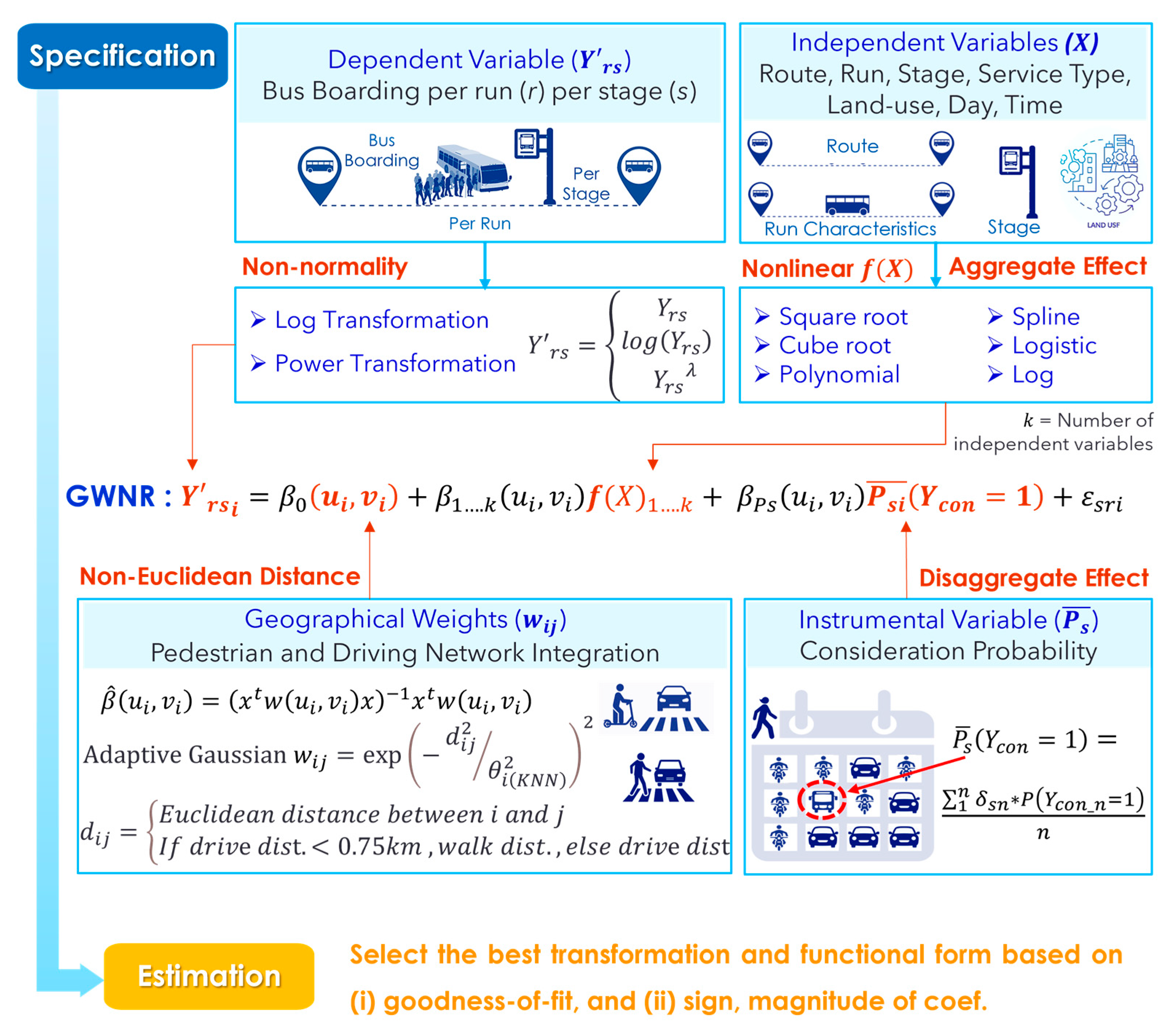
4. Methodology and Model Formulation

The proposed model formulation involves the following steps (Figure 2): (i) transforming boarding data for normality, (ii) applying nonlinear forms of key influencing factors, (iii) incorporating consideration probability, and (iv) deriving mode-specific spatial impedance metrics.

4.1. Transformation of the Response Variable for Normality

The response variable ($Y_{rs}$) in this paper is boarding per run (r) per stage (s). Logarithmic transformation is commonly used in the literature [4,12,14]. Therefore, $Y_{rs}$ is transformed using both logarithmic and power functions, with the optimal power parameter determined through the Box-Cox transformation, to evaluate the empirical distribution of the data (Equation (1)). Equation (2) presents the boarding model, where ${\beta }_0$ is the intercept, ${\beta }_1$ to ${\beta }_8$ are coefficients of the influencing factors (X) listed in Table 2, and ${\epsilon }_{sr}$ is the error term with a zero mean. The best model is determined by goodness-of-fit metrics such as adjusted R² and mean absolute error (MAE), and also the significance, signs, and magnitude of key influencing factors’ coefficients (β).

$${Y^{\prime }}_{rs}=\left\{\begin{array}{c}{Y}_{rs},inoriginalscaleusedinOLSasBenchmark\\ \mathit{log}\left(Y_{rs}\right),forlogtransformation(Box-Coxwith\lambda =0)\\ {Y_{rs}}^{\lambda },forpowertransformation(Box-Coxwith\lambda \ne 0)\end{array}\right.$$

(1)

$${Y^{\prime }}_{rs}={\beta }_0+{\beta }_1{SC}_s+{\beta }_2{RTC}_{rt}+{{\beta }_{3}RNC}_r+{\beta }_4{LC}_s+{{\beta }_{5}ST}_r+{{\beta }_{6}TD}_r+{{\beta }_{7}DW}_r+{{\beta }_{8}TW}_r+{\epsilon }_{sr}$$

(2)

4.2. Nonlinear Functional Forms for the Influencing Factors

Nonlinear transformations such as log, logistic, square root, cube root, spline, and polynomial are applied to the key influencing factors (X) with continuous variables, as defined in Table 2. These transformations are used to capture the practical complexity of the relationship between $Y_{rs}$ and its key influencing factors. The model’s adjusted R², MAE, and ${Y^{\prime }}_{sr}$ versus βx plot are used to determine the most appropriate function, denoted by f in Equation (3). The final transformation is selected to ensure the best predictive accuracy with easy interpretability and practical decision-making for transit operators by reflecting the real-world relationship between bus boardings per run per stage and its influencing factors.

$${Y^{\prime }}_{rs}={\beta }_0+{\beta }_1{f_1(SC}_s)+{\beta }_2{f_2(RTC}_{rt})+{{\beta }_3{f}_3(RNC}_r)+{\beta }_4{f_4(LC}_s)+{{\beta }_{5}ST}_r+{{\beta }_{6}TD}_r+{{\beta }_{7}DW}_r+{{\beta }_{8}TW}_r+{\epsilon }_{sr}$$

(3)

4.3. Inclusion of Bus Consideration Probability

A global binary logit model predicts the probability of bus consideration ($Y_{con\_n}$) for nth individual (Equation (4)). The utility of bus consideration ($U_{con\_n}$) comprises a systematic component $V_{con\_n}$ and random component ${ϵ}_{con\_n}$ (Equation (5)). $V_{con\_n}$ is explained by four sets of variables defined in Section 3 (Table 3), and γ denotes the set of coefficient vectors.

$$Y_{con\_n}=\left\{\begin{array}{c}1,ifbusisconsidered\\ 0,otherwise\end{array}\right.$$

(4)

$$U_{con\_n}=V_{con\_n}+{ϵ}_{con\_n}={\mathsf{\gamma }}_0+{\mathsf{\gamma }}_1{ACC}_n+{\mathsf{\gamma }}_2{NII}_n+{\mathsf{\gamma }}_3{TSC}_n+{\mathsf{\gamma }}_4{PWC}_n+{ϵ}_{con\_n}$$

(5)

The corresponding log-likelihood to estimate γ:

$$LL=\sum _1^n{Y}_{con\_n}\ast \log P\left(Y_{con\_n}=1\right)+(1-Y_{con\_n})\ast \log P\left(Y_{con\_n}=0\right)$$

(6)

Disaggregate consideration probability is used as an instrumental variable in the boarding model to overcome self-selection bias and capture the effect of all individuals’ perceptions and behaviors regardless of bus usage (Equation (7)). This instrumental variable ($\overline{P_s}$) is the average of predicted bus consideration probabilities only among those individuals who consider buses within a 500 m buffer around their home or work locations.

$$\overline{P_s}\left(Y_{con}=1\right)={\displaystyle \frac{\sum _1^n{\delta }_{sn}\ast P\left(Y_{con\_n}=1\right)}{n}}$$

(7)

where ${\delta }_{sn}=\left\{\begin{array}{c}1,ifindividualnbelongsto500\mathrm{m}bufferofbusstages\\ 0,otherwise\end{array}\right.$.

4.4. Mode and Distance-Specific Spatial Impedance Metric

Global regression models cannot effectively capture spatial variation because they assign uniform coefficients across the entire study area. In contrast, the GWR model addresses this limitation by computing geographical weights ($w_{ij})$ from neighboring data points to estimate coefficients for the $k^{\mathrm{t}\mathrm{h}}$ independent variable of a reference data point i at location $\left(u_i,v_i\right)$ (Equation (8)). In this way, GWR addresses spatial heterogeneity and autocorrelation. In the proposed GWNR, the best transformation of the dependent variable (${{Y^{\prime }}_{rs}}_i)$ (log vs. power) is used with the independent variables listed in Table 2 along with the average predicted bus consideration probability ($\overline{P_s}$).

$$\begin{array}{cc}\hfill {{Y^{\prime }}_{rs}}_i={\beta }_0\left(u_i,v_i\right)& +{\beta }_1{\left(u_i,v_i\right)f_1(SC}_{si})+{\beta }_2\left(u_i,v_i\right){f_2(RTC}_{rti})+{{\beta }_3\left(u_i,v_i\right)f_3(RNC}_{ri})+{\beta }_4{\left(u_i,v_i\right)f_4(LC}_{si})\hfill \\ \hfill & +{{\beta }_5\left(u_i,v_i\right)ST}_{ri}+{{\beta }_6\left(u_i,v_i\right)TD}_{ri}+{{\beta }_7\left(u_i,v_i\right)DW}_{ri}+{{\beta }_8\left(u_i,v_i\right)TW}_{ri}+{\beta }_9\left(u_i,v_i\right)\overline{P_{si}}\left(Y_{con}=1\right)\hfill \\ \hfill & +{\epsilon }_{sri}\hfill \end{array}$$

(8)

Calibration of this model involves optimizing the bandwidth, i.e., determining the extent of neighbor contributions to the estimation of the ith data point. Weights follow the distance–decay concept, and kernel functions quantify the contribution of neighboring data points to coefficient estimation. This allows for a local calibration of the regression model by moving the regression point spatially. The matrix $\widehat{\beta }\left(u_i,v_i\right)$ estimates the GWR parameter at location $\left(u_i,v_i\right)$ (Equation (9)).

$$\widehat{\beta }\left(u_i,v_i\right)={\left(x^{t}w\left(u_i,v_i\right)x\right)}^{-1}{x}^{t}w\left(u_i,v_i\right)$$

(9)

Four kernel functions namely fixed Gaussian, fixed bi-square, adaptive Gaussian, and adaptive bi-square, are commonly used for differential weighting. The adaptive kernel adjusts its bandwidth size ${\theta }_{i\left(KNN\right)}$ based on data point density, using the $K^{\mathrm{t}\mathrm{h}}$ nearest neighbor distance, while the fixed kernel maintains a constant bandwidth regardless of data density. The bi-square function employs a clear cut-off for neighboring contributions, whereas Gaussian function considers contributions from all neighbors with a diminishing effect based on distance. In the bandwidth selection process, neighboring data points are chosen based on the distance-decay concept within a defined range. If all data points are included, the model behaves like a global model. Conversely, if too few data points are included, the estimation may not converge properly. In this study, bandwidth selection is based on the cross-validation minimization technique, which identifies the lowest prediction error. Among the kernels tested, the adaptive Gaussian performed the best, and its adaptability has also been noted in previous studies [29].

$$\mathrm{A}\mathrm{d}\mathrm{a}\mathrm{p}\mathrm{t}\mathrm{i}\mathrm{v}\mathrm{e}\mathrm{G}\mathrm{a}\mathrm{u}\mathrm{s}\mathrm{s}\mathrm{i}\mathrm{a}\mathrm{n}=\mathrm{e}\mathrm{x}\mathrm{p}{\left(-{\displaystyle \raisebox{1ex}{$d_{\mathit{ij}}^2$}\!\left/ \!\raisebox{-1ex}{${\theta }_{i\left(\mathit{KNN}\right)}^2$}\right.}\right)}^2$$

(10)

Traditional GWR often uses Euclidean distance for geographical weights in regression models, which may oversimplify real-world impediments and neglect physical barriers [9]. Although some studies use metrics such as Minkowski, Manhattan, or shortest path distances [23,30], these often overlook actual geographic distances and mode feasibility for accessing bus stops. Walking may be more practical for shorter distances than driving, and pedestrian network distance may differ from driving network distance. Therefore, neighborhood contributions to estimation can also vary based on mode feasibility. In the proposed GWNR framework, the distance $\left(d_{ij}\right)$ between data points i and j (Equation (10)) is assessed as network distance based on mode feasibility to offer a more realistic representation of spatial heterogeneity and autocorrelation. The household survey in Chennai revealed that the 75th percentile access distance from home to bus stop for pedestrians is 0.75 km. Therefore, for distances under 0.75 km, the pedestrian network (local and collector streets) is used, while the driving network is applied for longer distances (Equation (11)). The weight contributed by neighbors in the estimation of reference points varies based on this mode-specific distance matrix.

$$d_{ij}=\left\{\begin{array}{c}\mathrm{Euclidean}\mathrm{distance}\mathrm{between}i\mathrm{and}j\\ \mathrm{If}\mathrm{driving}\mathrm{distance}<0.75\mathrm{km},\mathrm{walking}\mathrm{distance},\mathrm{else}\mathrm{driving}\mathrm{distance}\mathrm{between}i\mathrm{and}j\end{array}\right.$$

(11)

4.5. Model Execution

A runtime analysis was conducted to evaluate the computational feasibility of the GWNR model, as shown in Figure 3. The model was tested on a system with an Intel Core i7 (2.92 GHz, x64), 16 GB RAM, running Windows 11, using Python 3.9.13. The results show that runtime increases with dataset size but remains within practical limits even for large data sets and offline applications. With a multi-threaded setup using 16 threads, the model’s total runtime increased with dataset size: approximately 10 min for 5000 observations, 40 min for 15,000, 100 min for 25,000, and 300 min for 35,000 observations. The computational load increases primarily due to localized parameter estimation. However, the ‘SearchGWRParameter’ function facilitates parallel processing techniques using multi-threading and optimizes bandwidth, which significantly reduces computation time. Thus, even if GWNR is computationally intensive, it remains a feasible approach for larger transit networks with appropriate optimizations.

The above-discussed advancements in GWNR methodology are summarized in Figure 2. These advancements can enhance the responsiveness of the proposed boarding model to both aggregate and disaggregate characteristics and jointly address nonlinearity and spatial heterogeneity. The subsequent section explores the results and inferences drawn from this model.

5. Results and Discussion

5.1. Effect of Non-Normality of Boarding

Logarithmic and power transformations of bus boarding per run per stage were tested to evaluate empirical distribution and model fit. The Box-Cox transformation identified an optimal exponent (λ) of 0.494, which was rounded to 0.5 (square root) for ease of back-transformation. Among the tested transformations, the square root ($\sqrt{Y_{rs}}$) provided the best model fit, ensuring residual normality and achieving the highest adjusted R² (0.57), lowest MAE (2.22), and RMSE (3.32). This outperformed both the original scale $Y_{rs}$ (adjusted R² = 0.54, MAE = 2.31, RMSE = 3.40) and the logarithmic scale $log\left(Y_{rs}\right)$ (adjusted R² = 0.35, MAE = 3.61, RMSE = 4.20). Additionally, Q-Q plots and density plots of $\sqrt{Y_{rs}}$ confirm improved residual normality, with closer alignment to theoretical quantiles and more symmetrical density curves, validating this choice of transformation ($\sqrt{Y_{rs}}$) as the most suitable.

Figure 4 compares the normality and goodness-of-fit of six OLS global models in original versus square root scale, using Q-Q plots and density plots of standardized residuals. The Q-Q plots show how closely the standardized residuals follow a theoretical normal distribution, with better fits indicated by the yellow points/line closer to the red dashed line. The overlaid blue density curves on the histograms illustrate the standardized residuals’ distribution, with a bell-shaped curve indicating normality.

The plots indicate that models using the square root transformation of the response variable $Y_{rs}$ (bus boardings per run per stage) generally produce residuals that follow a normal distribution much more closely when compared to models using the original $Y_{rs}$. This is evident from improved alignment with theoretical quantiles and more symmetrical density curves in the bottom row plots. Specifically, the nonlinear model employing $\sqrt{Y_{rs}}$ (Figure 4f) achieves the highest adjusted R² (0.59), lowest MAE (2.16), and RMSE (3.23), indicating the best fit and most accurate predictions among all OLS global models.

The adjusted R² improved by 9.3% in the proposed nonlinear OLS model (0.59 in Figure 4f) from the traditional OLS model (0.54 in Figure 4a), indicating a substantially better fit. This shows that transforming the response variable, applying nonlinear functional forms, and including consideration probability as an instrumental variable can significantly improve model performance and normality of residuals with more robust statistical inferences.

From a behavioral perspective, further analysis reveals that the deviation between scheduled and observed headways ${(SCH\text{\_}HW-OBS\text{\_}HW)}_{sameroute}$ becomes significant at a 90% confidence level after applying a square root transformation to $Y_{rs}$, unlike the original scale (

Table 4. Summary of key global model results and effects of transformations.

Variables	Functional Form	Linear x with Original y		Linear x with √y		Nonlinear x with √y		Nonlinear x and Consideration with √y
		Coef	t Value	Coef	t Value	Coef	t Value	Coef	t Value
Route Characteristics
Scheduled headway with respect to the current route direction at a stage for the current time window (in minutes) 1	Cubic	−0.04	−4.14	−0.02	−6.25	9.84	6.76	12.82	8.91
						−1.14	−6.65	−1.51	−8.90
						0.04	6.51	0.06	8.83
Deviation between scheduled and observed headway with respect to the current route direction at a stage (in minutes) 2	Cubic	0.01	1.02	0.01	2.95	0.0002	0.01	0.002	0.14
						0.01	1.44	0.00	1.32
						−0.001	−2.23	−0.001	−2.12
Land-use Characteristics (within 500 m buffer)
Number of bus stations 3	Quadratic	−0.06	−6.26	−0.01	−5.92	−0.04	−3.73	0.03	3.41
						0.001	2.05	−0.004	−7.09
Number of train stations 3	Quadratic	0.77	13.84	0.24	16.05	0.24	5.09	0.51	10.78
						0.00	−0.19	−0.18	−7.19
Consideration Probability (within 500 m buffer)
Average of aggregated bus consideration probability for the people who considered bus 4	Linear							0.70	22.59
Missing values for bus consideration probability	Binary							0.73	26.71

¹ Coefficients show nonlinearity. ² Coefficient has a significant t value after applying the √y transformation. ³ Coefficients become intuitive after incorporating ‘Consideration Probability’. ⁴ Coefficient shows a positive effect of bus consideration probability on bus boarding.

). Additionally, applying nonlinear functional forms to explanatory variables and incorporating consideration probability makes the influence of some key explanatory variables, such as the number of bus stops and train stations, more logical and practically relevant, as discussed in the following Section 5.2. The key results from all models presented in Figure 5 are summarized in Table 4. To improve clarity and highlight significant improvements after transformation, the summary table presents only the most influential coefficients along with their interpretations. This summary table provides a clearer insight into the key relationships identified in the model, and the full numerical details are available in the Appendix A (

Table A1. Results from bus boarding models.

Variables	Functional Form	Linear x with Original y		Linear x with √y		Nonlinear x with √y		Nonlinear x and Consideration with √y		Euclidean GWR—Linear x with Original y		Non-Euclidean GWR—Non-Linear x and Consideration with √y
		Coef	Std Err	Coef	Std Err	Coef	Std Err	Coef	Std Err	Mean	Std Dev	Mean	Std Dev
Intercept		3.09	0.23	1.50	0.06	−24.19	3.80	−32.20	3.76	2.13	3.59	−15.84	34.22
Stage Characteristics
The starting stage of a route	Binary	11.29	0.13	2.30	0.03	2.16	0.05	2.00	0.05	12.06	1.88	1.20	0.71
The ending stage of a route		−0.91	0.12	−0.40	0.03	0.32	0.05	0.27	0.05	−2.00	2.40	−0.58	1.13
The intermediate stage of a route (base)
Stage Index = Position Number of Current Stage /Total Number of Stages	Cubic	−2.85	0.10	−1.08	0.03	−5.57	0.40	−6.51	0.40	−2.74	1.52	−12.08	3.80
						11.55	0.83	13.01	0.82			23.26	9.51
						−8.11	0.51	−8.75	0.51			−14.67	6.26
Route Characteristics
Deviation between bus and driving route distance (in km)	Quadratic	−0.11	0.01	−0.02	0.004	−0.05	0.03	−0.04	0.03	−0.29	0.30	−0.20	0.37
						0.01	0.002	0.005	0.00			0.02	0.01
Scheduled headway with respect to the current route direction at a stage for the current time window (in minutes)	Cubic	−0.04	0.01	−0.02	0.003	9.84	1.46	12.82	1.44	0.09	0.36	6.43	12.51
						−1.14	0.17	−1.51	0.17			−0.75	1.45
						0.04	0.01	0.06	0.01			0.03	0.05
Stage-level bus inter-arrival times for the current time window (in minutes)	Linear	0.01	0.003	0.004	0.001	0.002	0.001	0.002	0.001	0.01	0.004	0.004	0.002
Deviation between scheduled and observed headway with respect to the current route direction at a stage (in minutes)	Cubic	0.01	0.01	0.01	0.002	0.0002	0.01	0.002	0.01	0.03	0.003	0.04	0.004
						0.01	0.004	0.00	0.004			0.01	0.001
						−0.001	0.0001	−0.001	0.0001			−0.001	0.0001
Run Characteristics
Previous stage occupancy = (Cumulative boarding − cumulative alighting) up to the previous stage per run	Cubic	0.01	0.003	0.01	0.001	0.01	0.004	0.01	0.004	0.02	0.01	0.03	0.01
						−0.00005	0.001	−0.0001	0.001			−0.001	0.001
						−0.0000004	0.000	−0.000001	0.000			0.000003	0.000
Previous trip occupancy = (Cumulative boarding − cumulative alighting) at the current stage per run during the previous trip	Cubic	0.04	0.002	0.01	0.001	0.02	0.003	0.02	0.003	0.03	0.01	0.01	0.004
						−0.0003	0.0001	−0.0004	0.0001			0.0004	0.0001
						0.000003	0.0000	0.000003	0.0000			−0.000004	0.0000
Missing values for previous trip occupancy	Binary	0.57	0.17	0.11	0.04	0.20	0.05	0.23	0.05	1.29	0.40	0.13	0.28
Service Type
Ordinary	Binary	1.25	0.14	0.31	0.04	0.13	0.05	0.13	0.04	1.20	0.61	0.16	0.04
Deluxe		−1.60	0.07	−0.35	0.02	−0.38	0.02	−0.37	0.02	−1.61	0.56	−0.32	0.09
Express (Base)
Trip Direction (Away from central urban area: Base)
Towards central urban area	Binary	−0.01	0.05	0.01	0.01	0.08	0.02	0.08	0.02	0.26	1.15	0.34	0.37
Land-use Characteristics (within 500 m buffer)
Number of bus stations	Quadratic	−0.06	0.01	−0.01	0.002	−0.04	0.01	0.03	0.01	−0.13	0.10	0.03	0.16
						0.001	0.001	−0.004	0.001			−0.003	0.01
Number of train stations	Quadratic	0.77	0.06	0.24	0.02	0.24	0.05	0.51	0.05	1.31	0.84	0.72	6.69
						0.00	0.02	−0.18	0.03			−0.56	6.85
Number of educational institutes	Square root	0.09	0.004	0.01	0.001	0.15	0.01	0.13	0.01	0.15	0.12	0.24	0.12
Number of government offices	Cubic	−0.07	0.01	−0.02	0.002	−0.13	0.01	−0.09	0.01	−0.38	0.61	−0.21	0.48
						0.01	0.00	0.01	0.001			0.20	0.44
						−0.0004	0.00	−0.0004	0.00004			−0.01	0.03
Sparse land-use area	Binary	0.26	0.12	−0.23	0.03	−0.20	0.03	−0.18	0.03	0.35	1.81	−0.12	0.69
Neither sparse nor dense land-use area		0.73	0.09	0.09	0.02	0.10	0.02	0.09	0.02	1.19	1.46	0.38	0.48
Dense land-use area (base)
Land-use variable is missing		−0.25	0.16	−0.34	0.04	−0.26	0.05	0.07	0.06	−0.29	1.74	0.57	0.93
Day of Week
Monday (0/1)	Binary	−0.09	0.07	0.00	0.02	−0.01	0.02	−0.01	0.02	−0.33	0.08	−0.06	0.01
Tuesday (0/1)		0.12	0.07	0.04	0.02	0.03	0.02	0.03	0.02	0.31	0.05	0.08	0.01
Wednesday (0/1)		−0.09	0.07	−0.01	0.02	−0.03	0.02	−0.03	0.02	−0.24	0.04	−0.07	0.01
Thursday (0/1)		−0.02	0.07	0.02	0.02	0.02	0.02	0.02	0.02	−0.05	0.23	0.08	0.01
Friday (Base)
Time Window
6 a.m.–7 a.m. (Base)
7 a.m.–8 a.m.	Binary	0.74	0.12	0.17	0.03	0.18	0.03	0.15	0.03	0.83	0.46	0.21	0.11
8 a.m.–9 a.m.		1.38	0.14	0.27	0.04	0.30	0.04	0.27	0.04	1.27	0.61	0.30	0.11
9 a.m.–10 a.m.		0.96	0.14	0.15	0.04	0.18	0.04	0.15	0.04	1.08	0.41	0.21	0.10
10 a.m.–11 a.m.		0.49	0.13	0.07	0.03	0.08	0.03	0.06	0.03	0.70	0.29	0.14	0.06
11 a.m.–12 p.m.		0.26	0.13	0.05	0.03	0.03	0.03	0.02	0.03	0.52	0.23	0.11	0.07
12 p.m.–1 p.m.		0.37	0.13	0.08	0.03	0.08	0.03	0.07	0.03	1.23	0.46	0.27	0.11
1 p.m.–2 p.m.		0.20	0.13	0.03	0.03	0.04	0.03	0.03	0.03	0.68	0.12	0.15	0.02
2 p.m.–3 p.m.		0.04	0.13	0.01	0.03	0.002	0.03	−0.001	0.03	0.17	0.43	0.10	0.00
3 p.m.–4 p.m.		0.17	0.13	0.05	0.03	0.06	0.03	0.05	0.03	0.84	0.31	0.18	0.04
4 p.m.–5 p.m.		1.00	0.13	0.27	0.03	0.29	0.03	0.27	0.03	1.08	0.35	0.32	0.08
5 p.m.–6 p.m.		1.45	0.15	0.33	0.04	0.36	0.04	0.33	0.04	1.38	0.44	0.38	0.09
6 p.m.–7 p.m.		1.47	0.15	0.32	0.04	0.35	0.04	0.32	0.04	1.39	0.44	0.35	0.09
7 p.m.–8 p.m.		0.76	0.16	0.11	0.04	0.15	0.04	0.12	0.04	0.89	0.33	0.23	0.07
8 p.m.–9 p.m.		0.44	0.17	−0.01	0.05	0.04	0.05	0.02	0.04	0.80	0.25	0.19	0.11
9 p.m.–10 p.m.		0.57	0.18	0.00	0.05	0.06	0.05	0.06	0.05	1.27	1.17	0.12	0.30
Consideration Probability (within 500 m buffer)
Average of aggregated bus consideration probability for people who considered buses	Linear							0.70	0.03			0.40	1.41
Missing values	Binary							0.73	0.03			0.62	0.94

(Italics and small font) Insignificant variables at 95% two-tail confidence level

).

5.2. Effect of Nonlinear Influencing Factors on Bus Boarding

Various nonlinear transformations were tested to find the best fit for key continuous independent variables, including logarithmic, logistic, square root, cubic root, quadratic, cubic, and spline functions, as summarized in

Table A2. Comparative analysis of nonlinear transformations selection for model performance evaluation.

Variable	Log		Logistic		Square Root		Cube Root		Quadratic		Cubic		Spline		Final Transformation *	Reason
	Adj R2	MAE	Adj R2	MAE	Adj R2	MAE	Adj R2	MAE	Adj R2	MAE	Adj R2	MAE	Adj R2	MAE
Stage index	0.566	2.225	0.566	2.223	0.565	2.226	0.565	2.228	0.567	2.215	0.571	2.201	0.571	2.201	Cubic	Best fit, simple, easy interpretation, optimal value
Route distance deviation (bus - drive)	0.566	2.221	0.567	2.220	0.566	2.222	0.566	2.221	0.567	2.221	0.568	2.219	0.567	2.219	Quadratic	Highest Adj R², lowest MAE
Scheduled headway	0.563	2.227	0.568	2.217	0.563	2.226	0.568	2.218	0.568	2.218	0.569	2.216	0.569	2.216	Cubic	Best fit, simple, easy interpretation, optimal value
(Schd-Obs.) headway	0.565	2.224	0.565	2.224	0.563	2.226	0.565	2.225	0.566	2.223	0.566	2.222	0.565	2.225	Cubic	Highest Adj R², lowest MAE
Last stage occupancy	0.565	2.226	0.567	2.229	0.563	2.227	0.565	2.225	0.565	2.225	0.565	2.225	0.565	2.225	Cubic	No improvement over others, but consistent
Last trip occupancy	0.562	2.227	0.555	2.246	0.564	2.225	0.565	2.225	0.566	2.223	0.566	2.222	0.565	2.224	Cubic	Highest Adj R², lowest MAE
Bus station	0.565	2.224	0.564	2.225	0.565	2.224	0.565	2.224	0.565	2.225	Insignificant		0.566	2.220	Quadratic	Highest Adj R², lowest MAE
Train station	0.565	2.225	0.565	2.225	0.565	2.225	0.565	2.226	0.565	2.225	Insignificant		0.565	2.225	Quadratic	Highest Adj R², lowest MAE
School	0.559	2.231	0.552	2.241	0.563	2.226	0.560	2.229	Insignificant		Insignificant		Insignificant		Square root	Highest Adj R², lowest MAE
Govt. office	0.566	2.220	0.569	2.215	0.566	2.222	0.567	2.220	0.564	2.223	0.570	2.214	0.565	2.223	Cubic	Highest Adj R², lowest MAE

* The bold red digits indicate the highest Adj R² and lowest MAE for each variable transformation.

in the Appendix A. The final transformation for each variable was selected primarily based on adjusted R² and MAE, ensuring logical reasoning and practical decision-making for transit operators also played a role in choosing transformations that accurately represent the relationship between bus boardings per run per stage and its influencing factors.

For example, although both the cubic and spline transformations provided the best fit, the cubic transformation was chosen instead of the spline function for scheduled headway. The cubic function provided a better fit with a simpler mathematical form, making interpretation easier. Spline functions can introduce unnecessary complexity because they allow for sudden shifts in the relationship between variables. The cubic transformation avoids this issue by ensuring smooth and continuous behavior. The cubic function also allows transit agencies to find optimal values by setting the second derivative to zero. This helps to identify points where changes in headway have the greatest impact on boardings.

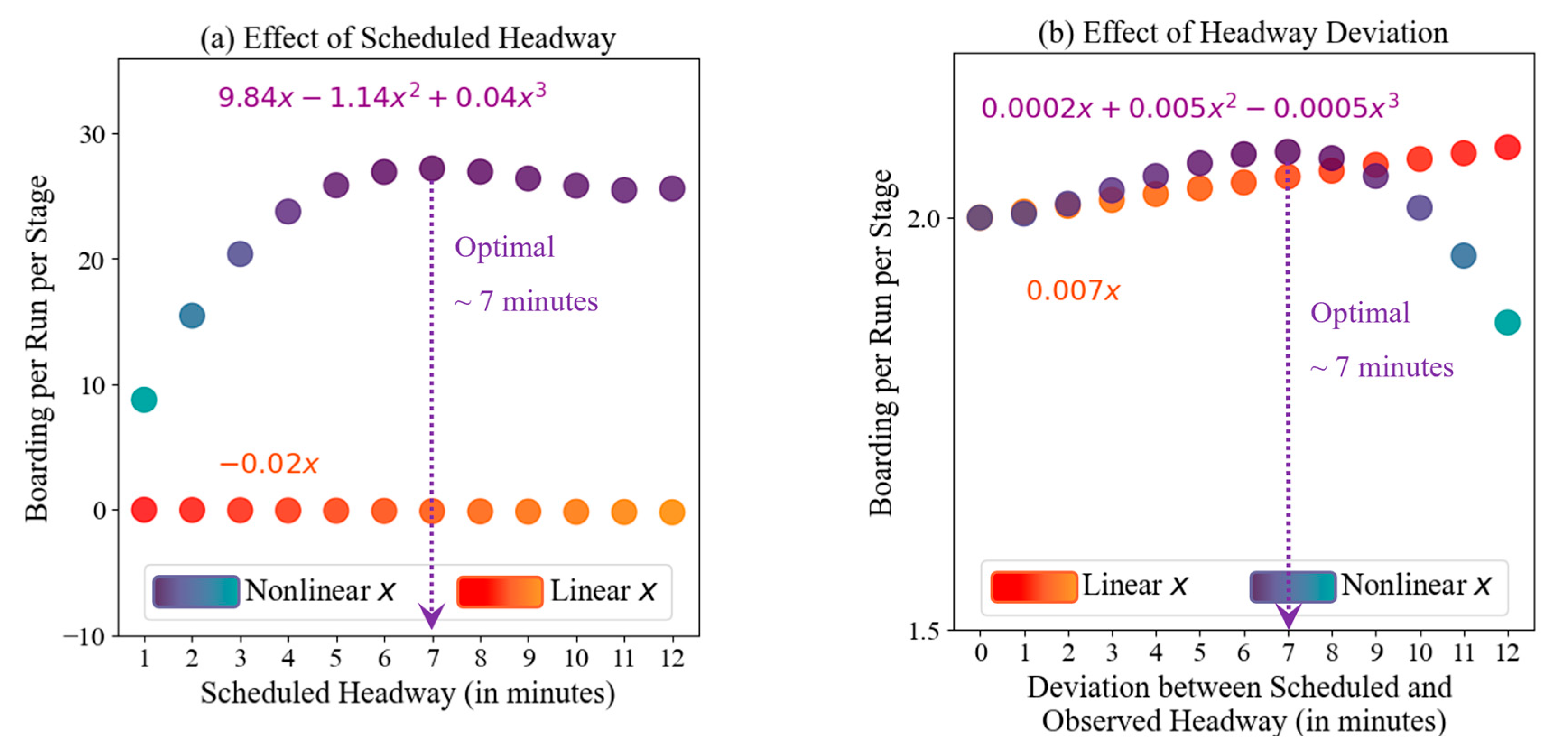
5.2.1. Nonlinear Effect of Scheduled Headway on Boarding

In Figure 5a, the linear function of scheduled headway $\left({SC{H}_{HW}}_{sameroute}\right)$ shows a negative impact on boarding per run per stage. The dark red dot indicates higher boarding values, and a yellowish-red dot indicates lower values, suggesting an impractical continuous increase in boarding as more buses arrive. In reality, with more buses, passengers tend to be distributed themselves more evenly across routes or services to avoid overcrowding, while too few buses can increase waiting times and potential mode shifts. Conversely, the cubic polynomial function provides a more realistic interpretation, showing an initial increase in boarding per run per stage (greenish-purple to dark purple dots in Figure 5a) with increased headway up to an optimal 7 min. Beyond this point, boarding declines for the given dataset. This pattern aligns with past studies by Alam et al. (2018) and Deepa et al. (2022), who found negative effects of bus headway on boarding or passenger miles, and a decrease in boarding benefits at high-frequency levels [4,14]. However, this study’s proposed cubic polynomial function finds an optimal scheduled headway of 7 min at the run level, which is not highlighted in past studies.

5.2.2. Nonlinear Effect of Headway Deviation on Boarding

When buses arrive earlier than scheduled, i.e., observed headway is shorter than scheduled headway ${(SCH\_HW-OBS\_HW)}_{sameroute}$, it can be beneficial up to a point. Early arrivals can accommodate passengers who missed the previous bus or arrived ahead of schedule. However, if buses arrive too early, boarding per run per stage may decrease due to fewer waiting passengers. In Figure 5b, the red dots represent the linear function, which misleadingly indicates a positive effect on boarding. In contrast, the polynomial function shows that an early arrival of up to 7 min (Figure 5b) can increase boarding (dark purple). Beyond this limit, a sharp decline in boarding occurs (greenish purple) for the given dataset. Thus, the cubic polynomial function is more practical as it identifies the optimal headway to enhance boarding.

5.3. Effect of Bus Consideration Probability on Bus Boarding

A binary logit bus consideration model with an AICc of 1012 and a ρ² of 0.13 is developed, with coefficients presented in

Table A3. Results obtained from the bus consideration model.

Variables	Global Binary Logit Model Coef. (Std. Error)
Intercept	0.13 (0.54)
Accessibility
Usability of footpath: Medium or high (1/0)	0.53 (0.17)
Usability of footpath: Missing (1/0)	0.54 (0.35)
Walking and crossing roads for buses are difficult and unsafe (1/0)	0.09 (0.19)
Small road density near home (in %)	−0.01 (0.01)
Network Integration
Direct bus is available to work (1/0)	1.08 (0.22)
Total walking time for transfers (in minutes)	0.02 (0.05)
Total walking time for transfers (in minutes) missing	−0.96 (0.35)
Access time to the nearest train station (in minutes)	0.01 (0.01)
Accurate information about bus routes is good (1/0)	0.39 (0.22)
Accurate information about bus timing is good (1/0)	0.53 (0.18)
Transit line haul service characteristics
Low security for women in bus (1/0)	−0.36 (0.21)
Low security for women in bus is missing (1/0)	0.50 (0.54)
Reliability of reaching on time by bus: Medium or high (1/0)	0.14 (0.17)
Crowd in bus is high or medium for bus line-haul distance ≤ 5 km (1/0)	−0.49 (0.23)
Crowd in bus is missing (1/0)	−0.63 (0.55)
Personal and work characteristics
Young Male (1/0)	0.32 (0.22)
Monthly household income before taxes is more than INR 20,000 (1/0)	−0.49 (0.17)
Come home for lunch (1/0)	−0.69 (0.26)
Travel at odd times (1/0)	0.17 (0.18)
Home to work Trip distance (in km) more than 15 km to 20 km (1/0)	0.19 (0.24)
Home to work Trip distance (in km) beyond 20 km (1/0)	0.70 (0.26)

in the Appendix A. A detailed interpretation of these coefficients is provided by Roy et al. (2024) [7]. In the square root nonlinear bus boarding model, the average predicted consideration probability from the binary logit model (within each stage’s 500 m buffer) is used as an instrumental variable. Its significant positive coefficient (0.70) indicates a beneficial impact on bus boarding (Table 4). This highlights the self-selection bias in the boarding model developed without this instrumental variable. Another notable difference between the models with (purple dots) and without (red dots) consideration probability is the relationship between land-use factors and boarding (Figure 6). The coefficients of the following two factors behave differently under each approach.

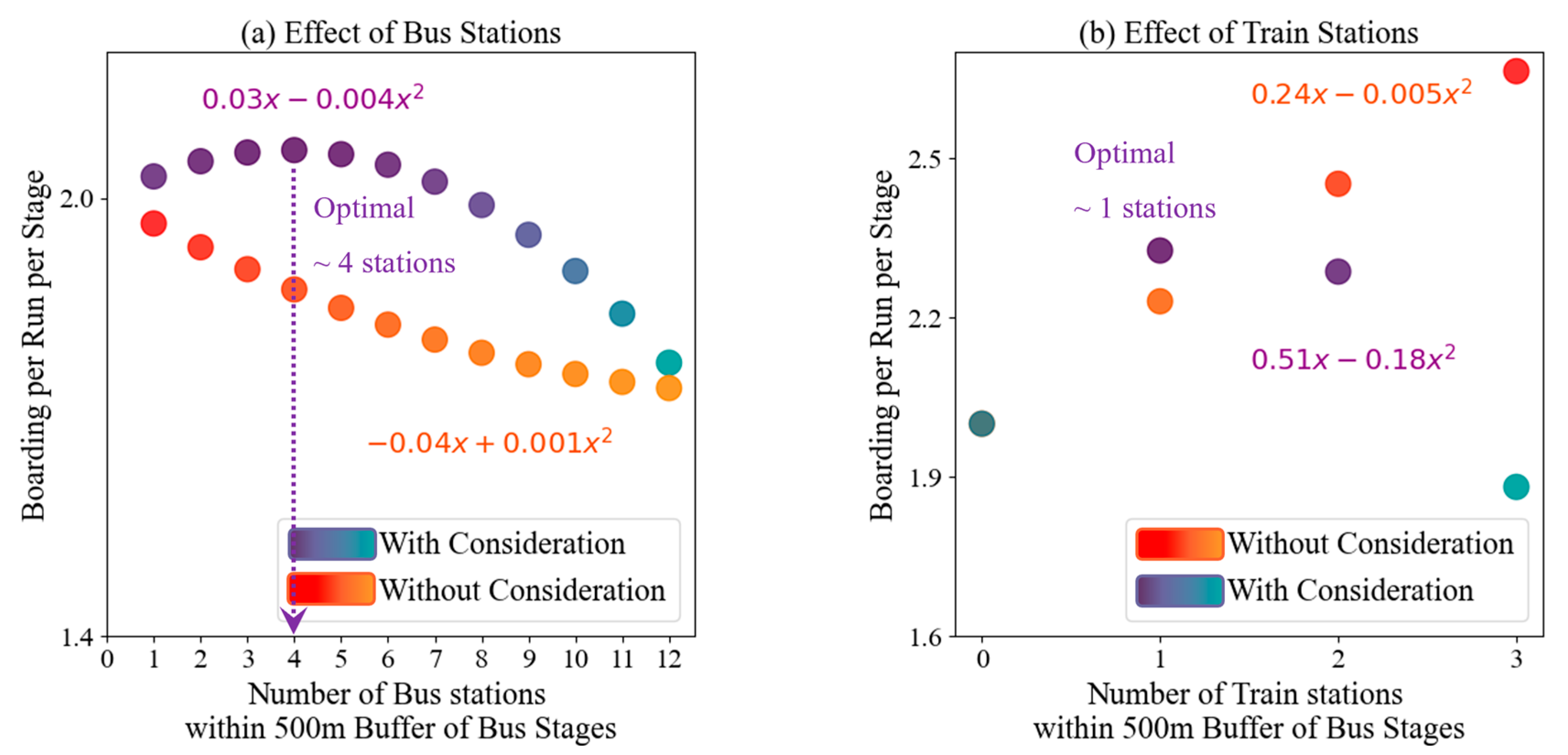
5.3.1. Effect of Bus Station Count Within a Buffer Area

Bus boarding per run per stage is expected to increase with the count of bus stations (${BS}_s$) upto a certain limit, after which passengers disperse to other nearby stops to avoid overcrowding. However, the boarding model without consideration probability produces an unrealistic decreasing trend. In contrast, the model incorporating consideration probability shows an increase in boarding (dark purple) with up to four bus stations within a 500 m buffer of a stage (Figure 6a), after which boarding declines (greenish purple). Previous research found a positive effect of the bus stops within a buffer on stop-route level hourly or daily boarding [13,22]. However, the proposed model stands out by focusing on run-stage level boarding results, showing different passenger distribution patterns beyond a certain number of bus stops.

5.3.2. Effect of Train Station Count Within a Buffer Area

Train stations within a 500 m buffer (${TS}_s)$ can either complement or compete with bus services. Rayaprolu and Levinson (2024) found that in Sydney, Australia, trains complement bus services by improving network connectivity, with well-planned transfers enhancing accessibility and reducing travel times [31]. On the other hand, Pei and Wang (2024) stated that in Harbin, China, rail transit competes strongly with conventional buses, attracting more passengers and causing bus ridership to decline. This is because trains have a larger capacity, higher speed, and are not affected by traffic congestion, making them a more convenient choice for many commuters [32]. Therefore, this relationship could be location-specific and is unpredictable beforehand. Despite this variability, there should be an optimal number of train stations to ensure complementarity. The model, without consideration of probability, suggests that bus boarding continuously increases with more train stations, which is illogical (yellowish to dark red dots in Figure 6b). Conversely, the model incorporating probability demonstrates that having one train station within the buffer enhances boarding (dark purple), by acting as a transfer point or increasing accessibility. Beyond this, additional train stations may compete with bus services (greenish purple), as rail systems are generally more reliable in terms of travel time.

The above observations highlight the importance of incorporating consideration probability in boarding models. The consideration-inclusive model more accurately reflects passenger behavior, suggesting optimal numbers of nearby bus and train stations to maximize boardings. Beyond these points, additional stations become less effective or reduce boardings due to passenger dispersion and increased competition from other transit modes.

Incorporating the square root transformation of boarding, nonlinear functional forms of influencing factors, and consideration probability as an instrumental variable makes the bus boarding OLS model statistically robust and behaviorally insightful. Thus, these features are also integrated into the GWR model for a better local behavioral perspective, as discussed below.

5.4. Local Effect of Influential Factors on Bus Boarding in GWR

Unlike past studies, the proposed model incorporates both pedestrian and driving networks to determine the distance metric in GWR. Specifically, a threshold of 0.75 km is used to select the network used to access bus stops. For distances under 0.75 km, the pedestrian network is used, while for longer distances, the driving network is applied. Despite the weight variation in neighbors’ contributions, the GWR model with Euclidean distance and the mode-specific network distance model produce nearly equivalent results due to the minimal difference between Euclidean and network distances in the study area. Similar findings are also reported by Guo and Bhat (2007) and Schirmer et al. (2014) [10,11]. Nevertheless, since using network distance is generally correct practice to better reflect real-world spatial heterogeneity compared to Euclidean distance, this study uses mode-specific network distance.

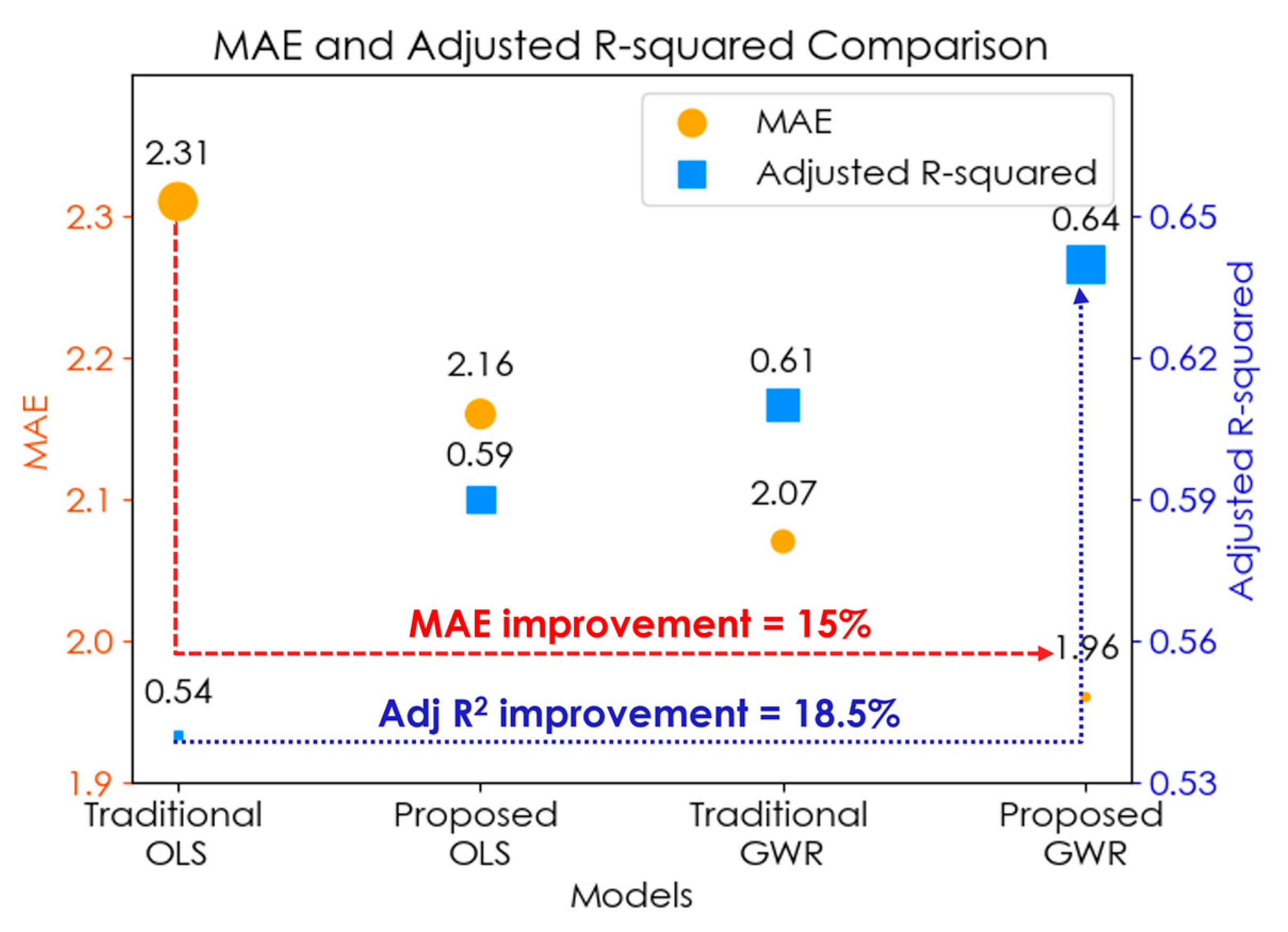
The proposed GWR model ($\sqrt{Y_{rs}}$ with nonlinear x, probability consideration, and mode-specific network distance) substantially improves goodness-of-fit compared to traditional OLS, proposed nonlinear OLS ($\sqrt{Y_{rs}}$ with nonlinear x and probability consideration), and traditional GWR (Figure 7). MAE values (shown as red dots) decrease from 2.31 in traditional OLS to 1.96 in the proposed GWR, indicating a 15% improvement. Adjusted R² (shown as blue squares) increases from 0.54 in traditional OLS to 0.64 in the proposed GWR, reflecting an 18.5% enhancement.

Effect of Influential Factors on Bus Boarding

Table 4 presents the results of all the developed OLS and GWR bus boarding models, incorporating both linear and nonlinear functional forms. Among these, the proposed GWR model, i.e., non-Euclidean GWR—nonlinear x and consideration with $\sqrt{Y_{rs}}$—shows superior goodness-of-fit compared to the other models in this study. The coefficients of influential variables derived from this model are analyzed to examine their impact on bus boarding per run per stage along bus routes in Chennai, India. Figure 8, Figure 9, Figure 10 and Figure 11 represent key influencing variables’ normalized coefficients (β), which indicate the strength of each variable’s effect, scaled from 0 to 1 based on their minimum and maximum values with a 90% confidence level (|t-values| ≥ 1.64). These β values are shown in different colors on spatial maps using QGIS: yellow for weak effects (0–0.25), green for moderate effects (0.26–0.50), sky blue for strong effects (0.51–0.75), and royal blue for very strong effects (0.76–1). Linear or binary influential variables exhibit positive or negative effects, seen in the green and red striped areas in Figure 9 and Figure 11. This behavior is typically observed in traditional GWR models. However, nonlinear influential variables have not been explored in past GWR studies. In this paper, Figure 8 and Figure 10 illustrate that the effects of these variables on bus boarding are not straightforwardly positive or negative. Instead, they have optimal values in a particular range, beyond which their effects change. These optimal values can vary by location. Even if the optimal values are the same across locations, their impact on boarding can vary across different places; in some places, the impact is high, while in others, it is not as significant.

Among stage characteristics, the starting stage positively impacts boarding, while the ending stage negatively influences, as expected. The cubic polynomial form of the stage index indicates higher boarding at stages near transit hubs or major trip production points and lower boarding at stages with fewer production points, which is intuitive. Thus, the ‘optimal’ stage index can guide strategic planning for station amenities to maximize boarding levels.

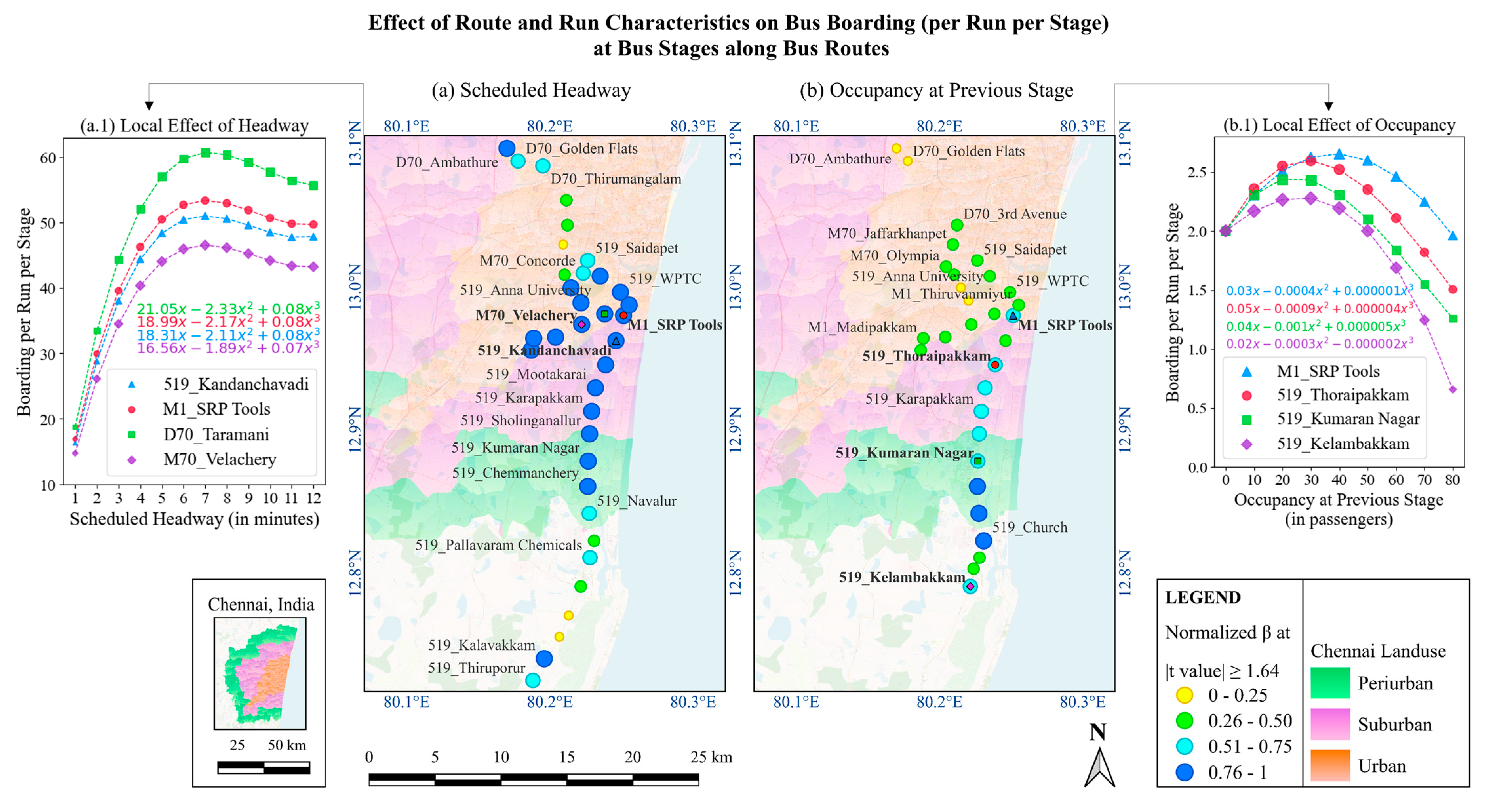
Route characteristics, such as the deviation between bus and driving route distances affect boarding, but not always negatively as the linear model shows. High deviation can enhance boarding when routes traverse dense land use or major attractions. A quadratic function better explains these scenarios. Figure 8a shows that nonlinearity in scheduled headway reveals excessively frequent bus arrivals lead to sparse passenger boarding per run per stage, while overly infrequent arrivals result in prolonged waiting times. Polynomial functions identify an optimal headway that balances these extremes. Bus stages farther from the CBD, with higher β values (royal blue), are more affected by bus frequency due to reliance on buses in the absence of rail services. Figure 8(a.1) shows boarding peaks at a headway of 6 to 7 min at some stages (Kandanchavadi, SRP Tools, Taramani, and Velachery) along routes 519, M1, D70, and M70, respectively. However, suburban stages like Kandanchavadi and SRP Tools experience a higher boarding increase with headway compared to stages closer to the CBD.

Run characteristics, such as high occupancy at the previous stage and trip influence boarding positively in a linear model, may not always hold. People may choose different transport modes or wait for the next bus depending on their schedules, flexibility, and level of comfort. The polynomial function captures these practical interpretations better than the linear ones. Figure 8b shows stronger effects of occupancy at the previous stage on bus boarding in peri-urban and suburban areas (royal and sky blue). In Figure 8(b.1), SRP Tools on route M1 near the CBD shows peak boarding with previous stage occupancy of around 40 passengers. However, stages farther from the CBD, like Thoraipakkam, Kumaran Nagar, and Kelambakkam on route 519, show similar patterns with lower optimal values of 20 to 30 passengers, indicating peri-urban and suburban areas are more sensitive to overcrowding due to longer commutes to the CBD.

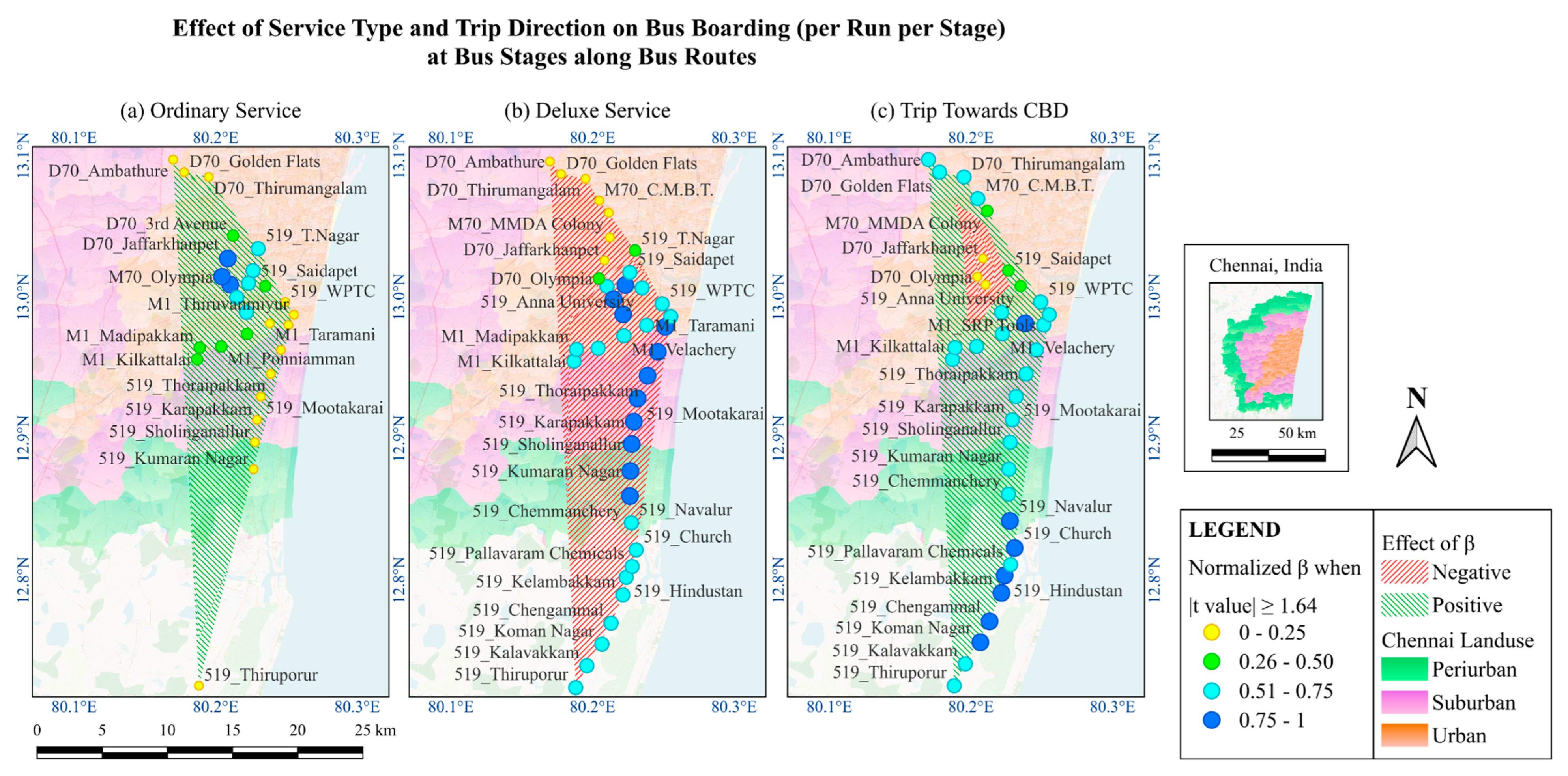
Cost sensitivity among bus passengers is evident as the cheapest ordinary bus service experiences the highest boarding levels, while the most expensive deluxe service has the least boarding. The express bus service boardings fall between these extremes. Figure 9a shows that ordinary bus services positively impact (green-striped areas) boarding everywhere, especially in CBD areas (royal and sky blue). Conversely, Figure 9b indicates that deluxe bus services have a stronger negative effect (red-striped) than ordinary services, particularly in suburban and urban areas. This trend suggests that passengers in these regions are more cost-sensitive and less inclined to choose premium services. Figure 9c shows that trips toward the CBD strongly increase boarding in peri-urban and suburban areas, as the CBD is a major destination with a high concentration of employment, commercial activities, and amenities.

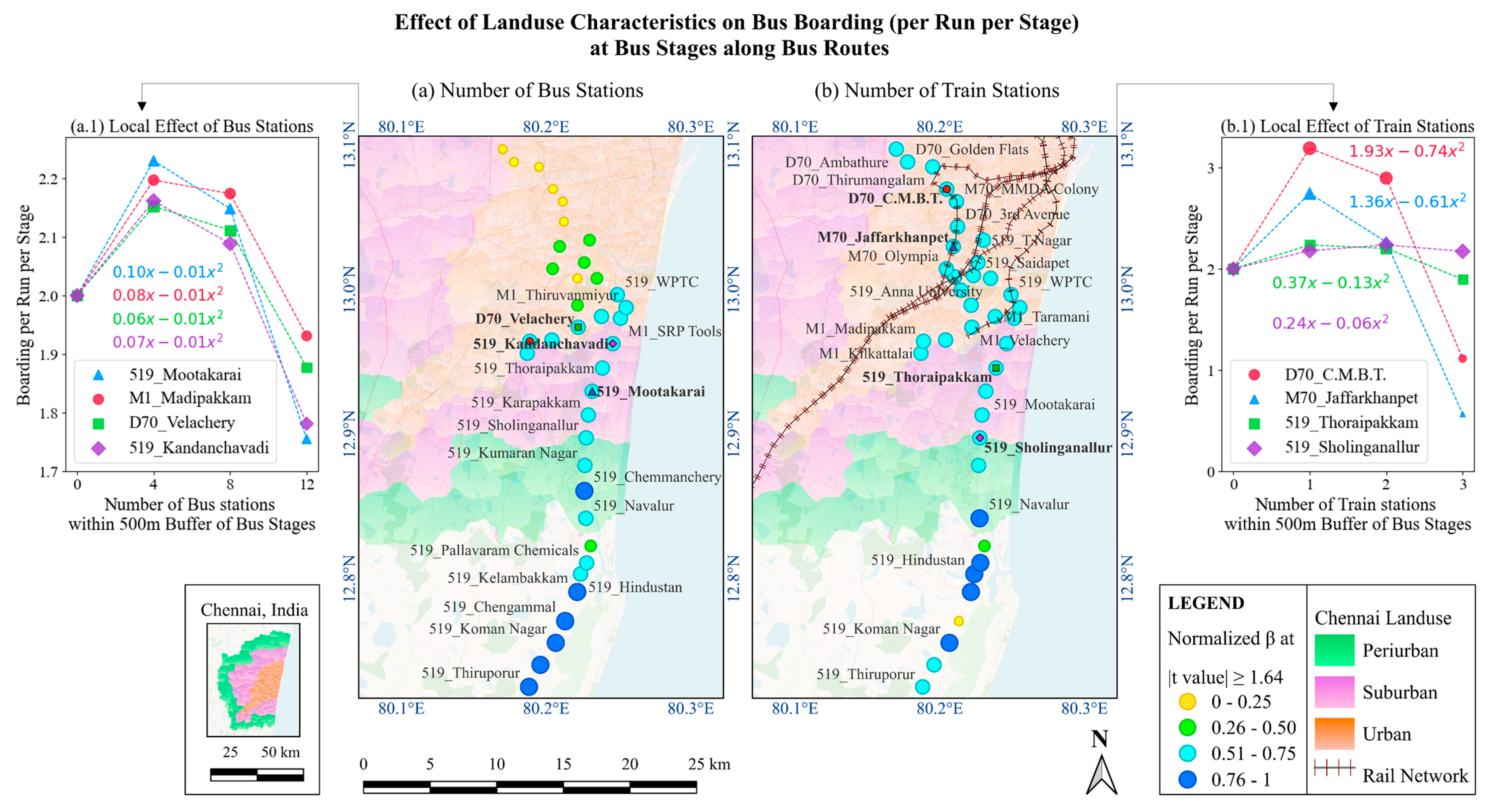
Figure 10a shows a strong local nonlinear effect of bus stations within 500 m on boarding in suburban and peri-urban areas that especially rely on buses. The plots in Figure 10(a.1) indicate that having too many nearby bus stops may not significantly increase boarding per run per stage, as passengers distribute themselves to avoid overcrowding, with boarding maximizing at up to four bus stations. Figure 10(b.1) shows that too many nearby train stations may reduce bus boardings due to competition, but up to one train station within 500 m can increase boardings due to integrated transport networks.

Regarding land use, sparse areas negatively affect boarding, whereas denser areas have a positive effect (Figure 11a,b). These effects are more pronounced in peri-urban areas, where land use is relatively sparser than the CBD.

Consideration probability consistently shows a strong positive effect on bus boarding across most locations (Figure 11c). This indicates that stages with higher consideration probabilities experience more bus boarding, likely due to increased public awareness and preference for these stages. This highlights the importance of taking into account both bus users’ and non-users’ behavior in the bus boarding prediction.

Among these selected routes, Wednesdays show the most significant negative impact on boarding compared to Fridays, possibly due to increased trips anticipated before the weekend. The peak hours from 7–9 a.m. and 4–8 p.m. have the highest positive effect on boarding.

6. Practical Applications

As discussed in Section 5.4, the proposed GWNR model can prioritize intervention locations with higher coefficients and identify the quantum of improvements needed to enhance bus ridership using polynomial functions. It finds facility requirements in prioritized locations with suboptimal facilities, which provides targeted policy guidance. In contrast, the proposed nonlinear OLS can determine the necessary improvements without prioritizing locations, while traditional GWR can prioritize locations but cannot identify the needed improvements; traditional OLS can do neither. This section compares the ridership gains from interventions aimed at improving bus scheduled headway using the nonlinear OLS and GWNR models to those achieved with traditional models.

Here, ridership refers to the total number of passengers boarding across all stages of a bus run. The policy intervention process is simulated by improving the scheduled headway of sample bus stages using the following mathematical calculations.

(a) Traditional OLS Model: In this model, the linear functional form of scheduled headway can find an extreme solution (maximum or minimum) within budget constraints based on the coefficient’s sign. However, it cannot determine the exact optimal headway value or prioritize improvement locations to maximize ridership. Moreover, regardless of location, it consistently shows a negative coefficient, which suggests increased bus boarding per run per stage with continuous reductions in scheduled headway, whereas, in practice, continuous reductions in headway can lead to frequent empty bus runs, causing significant losses for transit operators. Therefore, this policy analysis sets the headway reduction threshold at the 85th percentile of scheduled headways (i.e., 10 min per hour) in the study dataset. This 10-min headway may not provide the maximum benefit, but since the model does not provide any optimal value, this value is chosen within the range of feasible options. Fourteen out of 55 bus stages along sample bus routes have headways exceeding this threshold (shown in green dots in Figure 12a), and headways at these stages are subsequently improved by a 2-min reduction to meet the threshold limit.

(b) Traditional GWR Model: This model uses a linear functional form for scheduled headway and generates different coefficient values across locations. It also cannot find an optimal value but can prioritize improvement locations based on higher coefficient values, which indicates a stronger influence of scheduled headway on bus boardings at those locations. Similar to traditional OLS, in this model as well the headway reduction threshold is set at the 85th percentile of scheduled headways (i.e., 10 min per hour) in the study dataset. Thirteen bus stages along sample bus routes have headways exceeding this threshold (highlighted as green dots in Figure 12b), and headways at these stages are subsequently decreased by 2 min in priority order to meet the threshold limit.

(c) Proposed Nonlinear OLS Model: This model employs a cubic polynomial functional form of scheduled headway to find an optimal value providing maximum benefit. However, since it generates consistent coefficients across all locations, it cannot prioritize improvement locations to maximize ridership. Regardless of location, it identifies an optimal scheduled headway of 7 min per hour. If headway is reduced below this threshold, it leads to frequent empty bus runs, resulting in significant losses for transit operators. Conversely, increasing headway above 7 min creates prolonged passenger waiting times and can lead to mode shifts to alternative travel modes, also causing losses for bus transit operators. Therefore, the headway reduction threshold is set at 7 min per hour. Forty-two out of 55 bus stages along sample bus routes have headways exceeding this threshold, and headways at these stages are subsequently improved by reducing them by 2, 3, and 5 min (shown as green, blue, and red dots, respectively, in Figure 12c) to meet the threshold limit.

(d) Proposed GWNR Model: This model uses a cubic polynomial functional form of scheduled headway to find an optimal value and generates different coefficient values across locations, allowing it to prioritize improvement locations based on higher coefficients. Therefore, the headway reduction threshold is set at this optimal value. Locations with a very strong influence on scheduled headway (normalized β > 0.75) are prioritized for improvement. Fifteen priority bus stages along sample bus routes have headways exceeding their location-specific threshold, and headways at these stages are improved by reducing them by 2, 3, and 5 min (shown as green, blue, and red dots, respectively, in Figure 12d). This model provides a location-specific quantum of improvements, such as reducing the scheduled headway at ‘Taramani’ by 2 min for route M1 but by 5 min for route M70.

Bus boardings per run per stage are calculated using all four models, i.e., traditional OLS, traditional GWR, proposed OLS, and proposed GWR, with their respective improved headway values and original coefficients. Then, ridership per run is calculated, followed by the average ridership per hour per day. Similarly, the frequency of bus service is calculated from the scheduled headway before and after improvement for each model to determine how many buses are needed per hour per day. The bus frequency improvement ratio is calculated as follows:

$$BusFrequencyImprovementRatio={\displaystyle \frac{Totalincreaseinbusrunsperdayafterimprovement}{Totalbusrunsperdaybeforeimprovement}}$$

(12)

The bus ridership improvement ratio is calculated as:

$$BusRidershipImprovementRatio={\displaystyle \frac{Totalincreaseinridershipperdayafterimprovement}{Totalridershipperdaybeforeimprovement}}$$

(13)

Finally, the ridership gain index is calculated as:

$$RidershipGainIndex={\displaystyle \frac{BusRidershipImprovementRatio}{BusFrequencyImprovementRatio}}$$

(14)

Table 5. Ridership gain from traditional and proposed models.

Model		Bus Ridership Improvement Ratio	Bus Frequency Improvement Ratio	Ridership Gain Index
Traditional Models	OLS	0.005	0.034	0.147
	GWR	0.007	0.034	0.206
Proposed Nonlinear Models	OLS	1.022	0.295	3.464
	GWR	0.446	0.073	6.110

demonstrates the superior performance of the proposed GWNR model compared to both traditional models and the proposed OLS model. When traditional OLS and GWR models produce low ridership gain indices (0.147 and 0.206, respectively), the proposed models show substantial enhancements. The proposed OLS model achieves a notable ridership gain index of 3.552, while the proposed GWNR model achieves almost twice that, at 6.110. Hence, targeted interventions obtained from the proposed GWNR become twice as effective compared to those from traditional regression for maximizing bus ridership gains. In this study, the effectiveness of service planning policies is measured using the Ridership Gain Index, which evaluates how efficiently service enhancements translate into increased ridership. Transit agencies can utilize GWNR predictions to adjust bus schedules, improving service efficiency and promoting greater public transit usage, ultimately contributing to sustainable urban mobility.

Nonetheless, implementing these recommendations in real-world transit operations is not a standalone action. Adjusting scheduled headways for specific routes requires a holistic approach that accounts for multiple interdependent factors. For instance, operational constraints such as depot capacities, driver shift regulations, and fleet availability can limit how much a schedule can be altered without disrupting the overall system’s service reliability. Additionally, interactions between different routes play a crucial role because some routes may act as complements (facilitating seamless transfers) or competitors (serving overlapping demand), which may lead to passenger demand fluctuations. Given these complexities, transit agencies must assess the broader network-wide impacts before implementing service changes. Future research can explore scenario-based feedback mechanisms or simulation-driven approaches to understand the comprehensive effects of adjustments across the entire transit network in real-world applications.

7. Conclusions

This paper evaluates the role of nonlinearity and spatial heterogeneity in bus boarding in terms of prediction accuracy, behavioral relationships, and policy implications. A novel geographically weighted nonlinear regression (GWNR) model is developed to predict bus boardings at the run-stage level. This proposed model integrates aggregate ETM data from four MTC bus routes with disaggregate household survey data in Chennai to effectively capture both the bus users’ and non-bus users’ behavior. The proposed GWNR model improves the adjusted R-square by 18.5% and the mean absolute error by 15% compared to global linear regression.

This paper addresses all the research questions raised in the introduction section. First, it explores how appropriate functional forms of influencing factors can explain their relationship with bus boarding. A square root transformation ensures normality in the boarding data distribution. Contrary to many studies, this paper applies diverse nonlinear functions (e.g., power, polynomial, log, logistic, spline), among which the polynomial function provides the best fit and realistically depicts the relationship between most of the key influencing factors and bus boarding per run per stage. Linear models unrealistically suggest passenger boarding keeps increasing with more buses, whereas the proposed nonlinear model uses a cubic polynomial function to find an optimal 7-min headway for maximizing boarding along these sample routes. This creates a realistic balance, as more buses distribute passengers evenly to avoid overcrowding, while too few buses increase waiting times and cause people to switch to other travel modes. Such realistic behavioral insights are drawn from the nonlinear functional forms, and the optimal values help evaluate the quantum of improvements needed to enhance bus demand.

To address self-selection bias, the model includes bus consideration probability, predicted from a logit model with disaggregated household survey data, as an instrumental variable. This variable captures non-bus users’ behavior and examines how an individual’s consideration propensity affects the relationship between other factors and bus boarding. Incorporating this probability alters the relationship between land-use factors and boarding, presenting a more realistic pattern: boarding increases with more bus stations initially but declines due to passenger dispersion, while one train station enhances boarding, with additional stations creating competition.

Unlike prior research on GWR, this paper utilizes a mode-specific network distance metric to better represent neighborhood effects, providing area-specific insights into how station, route, run, land-use characteristics, and consideration propensity affect bus boarding. For instance, headways affect stages farther from the CBD due to reliance on bus service in the absence of rail. Previous stage occupancy influences boarding in peri-urban and suburban areas, where commutes to the CBD are longer. The number of nearby bus and train stations affects boarding, especially in suburban or peri-urban areas. Consideration probability consistently enhances boarding everywhere, highlighting the importance of perceived service reliability and convenience.

Finally, this paper compares ridership gains from policy interventions using the proposed GWNR model to those from traditional OLS and GWR, as well as nonlinear OLS models. The GWNR model prioritizes high-coefficient locations for interventions and optimizes the quantum of improvements using polynomial functions in suboptimal areas, providing targeted policy guidance to maximize ridership. Traditional OLS and GWR models achieve low ridership gain indices of 0.147 and 0.206, respectively. In contrast, the proposed nonlinear OLS model reaches a gain index of 3.552, and the GWNR model achieves an impressive 6.110, making interventions nearly twice as effective compared to traditional and global nonlinear methods. This enhanced effectiveness supports sustainability by maximizing ridership through targeted interventions, which can promote more efficient and resilient public transport systems.

Moreover, the proposed GWNR model is transferable to other cities according to its variable specifications, which account for transit infrastructure, land-use characteristics, service supply measures, and sociodemographic factors. The number of bus and train stations within a 500 m buffer of each stage represents transit infrastructure or transit stop density. The number of educational institutes and government offices within the same buffer captures land-use characteristics. Additionally, binary variables indicating whether the density of points of interest within a 500 m buffer is sparse or dense help differentiate low-density and high-density areas. Furthermore, scheduled headway for a specific route and stage-level bus inter-arrival times reflects service supply measures. The average bus consideration probability within a 500 m buffer of the current stage accounts for sociodemographic variations such as age, gender, income, and trip distance, as well as user perceptions of public transportation, including reliability, crowding, security, and usability of pedestrian infrastructure. Thus, given this structure, the GWNR model can be transferred to other cities by adjusting these variable values based on local conditions. However, due to spatial heterogeneity, some localized adjustments in bandwidth selection and calibration may be necessary to account for city-specific variations. Future research can further explore the model’s adaptability by applying it to develop a multi-city demand model with distinct transit characteristics. This would allow for validation of its generalizability using more direct measures, such as population density, employment accessibility, and other relevant factors across diverse urban contexts.

Furthermore, the proposed GWNR model can offer extensive applications across various fields by providing a valuable decision-making tool for realistic spatial analysis of demand, incorporating both aggregate and disaggregate characteristics. Beyond transportation, this model can significantly contribute to urban planning and retail. In urban planning, it can guide infrastructure development by identifying regions with high population growth and demand for amenities and providing targeted investment guidance in housing, schools, and public facilities. In retail, it can help in selecting store locations and designing marketing strategies by analyzing consumer behavior and identifying high-demand zones. Hence, the versatility of this model supports targeted and data-driven interventions across diverse sectors.

References

- Mead, L. Still Only One Earth: Lessons from 50 Years of UN Sustainable Development Policy. In The Road to Sustainable Transport Key Messages and Recommendations; International Institute for Sustainable Development: Winnipeg, MB, Canada, 2021. [Google Scholar]
- Erhardt, G.; Mucci, R.; Cooper, D.; Sana, B.; Chen, M.; Castiglione, J. Do Transportation Network Companies Increase or Decrease Transit Ridership? Empirical Evidence from San Francisco. Transportation 2021, 49, 313–342. [Google Scholar] [CrossRef]
- Bakar, M.; Norhisham, S.; Katman, H.; Fai, C.; Azlan, N.; Samsudin, N. Service Quality of Bus Performance in Asia: A Systematic Literature Review and Conceptual Framework. Sustainability 2022, 14, 7998. [Google Scholar] [CrossRef]
- Alam, B.M.; Nixon, H.; Zhang, Q. Factors Affecting Travel Demand by Bus: An Empirical Analysis at U.S. Metropolitan Statistical Area Level. Transp. Res. Rec. 2018, 2672, 817–826. [Google Scholar] [CrossRef]
- Diab, E.; DeWeese, J.; Chaloux, N.; El-Geneidy, A. Adjusting the Service? Understanding the Factors Affecting Bus Ridership Over Time at the Route Level in Montréal, Canada. Transportation 2021, 48, 2765–2786. [Google Scholar] [CrossRef]
- Ambi Ramakrishnan, G.; Srinivasan, K.K.; Pynda, S.P. Joint Models for Consideration of Public Transit and Mode Choice for Work Commute. Transp. Dev. Econ. 2020, 6, 12. [Google Scholar] [CrossRef]
- Roy, P.; Srinivasan, K.K.; Ramakrishnan, G.A. Why Don’t More Commuters Consider Buses for Their Work Trip?—A Geographically Weighted Segmented Logistic Regression Modelling Approach. Appl. Spat. Anal. 2024, 17, 1043–1079. [Google Scholar] [CrossRef]
- Rahman, M.; Yasmin, S.; Faghih-Imani, A.; Eluru, N. Examining the Bus Ridership Demand: Application of Spatio-Temporal Panel Models. J. Adv. Transp. 2021, 2021, 1–10. [Google Scholar] [CrossRef]
- Saputro, D.R.S.; Muhsinin, R.Y.; Widyaningsih, P.; Sulistyaningsih. Spatial Autoregressive with a Spatial Autoregressive Error Term Model and Its Parameter Estimation with Two-Stage Generalized Spatial Least Square Procedure. J. Phys. Conf. Ser. 2019, 1217, 012104. [Google Scholar] [CrossRef]
- Guo, J.Y.; Bhat, C.R. Operationalizing the Concept of Neighborhood: Application to Residential Location Choice Analysis. J. Transp. Geogr. 2007, 15, 31–45. [Google Scholar] [CrossRef]
- Schirmer, P.M.; van Eggermond, M.A.B.; Axhausen, K.W. The Role of Location in Residential Location Choice Models: A Review of Literature. J. Transp. Land Use 2014, 7, 3–21. [Google Scholar] [CrossRef]
- Cui, B.; DeWeese, J.; Wu, H.; King, D.A.; Levinson, D.; El-Geneidy, A. All Ridership Is Local: Accessibility, Competition, and Stop-Level Determinants of Daily Bus Boardings in Portland, Oregon. J. Transp. Geogr. 2022, 99, 103294. [Google Scholar] [CrossRef]
- Dong, X. Investigating Changes in Longitudinal Associations between Declining Bus Ridership, Bus Service, and Neighborhood Characteristics. J. Public Transp. 2022, 24, 100011. [Google Scholar] [CrossRef]
- Deepa, L.; Rawoof Pinjari, A.; Krishna Nirmale, S.; Srinivasan, K.K.; Rambha, T. A Direct Demand Model for Bus Transit Ridership in Bengaluru, India. Transp. Res. Part A Policy Pract. 2022, 163, 126–147. [Google Scholar] [CrossRef]
- Chakour, V.; Eluru, N. Examining the Influence of Stop Level Infrastructure and Built Environment on Bus Ridership in Montreal. J. Transp. Geogr. 2016, 51, 205–217. [Google Scholar] [CrossRef]
- Outwater, M.; Sana, B.; Ferdous, N.; Woodford, B.; Lobb, J. Characteristics of Premium Transit Services That Affect Choice of Mode; The National Academies Press: Washington, DC, USA, 2014. [Google Scholar]
- Mamede, F.P.; da Silva, R.F.; de Brito Junior, I.; Yoshizaki, H.T.Y.; Hino, C.M.; Cugnasca, C.E. Deep Learning and Statistical Models for Forecasting Transportation Demand: A Case Study of Multiple Distribution Centers. Logistics 2023, 7, 86. [Google Scholar] [CrossRef]
- Seyedan, M.; Mafakheri, F.; Wang, C. Cluster-Based Demand Forecasting Using Bayesian Model Averaging: An Ensemble Learning Approach. Decis. Anal. J. 2022, 3, 100033. [Google Scholar] [CrossRef]
- Wu, H.; Levinson, D. The Ensemble Approach to Forecasting: A Review and Synthesis. Transp. Res. Part C Emerg. Technol. 2021, 132, 103357. [Google Scholar] [CrossRef]
- Shakespeare, R.M.; Srinivasan, S. Demographic and Built Environment Predictors of Public Transportation Retention and Work-from-Home Changes in Small- to Medium-Sized Massachusetts Cities, 2011–2021. Sustainability 2024, 16, 8620. [Google Scholar] [CrossRef]
- Ma, X.; Zhang, J.; Ding, C.; Wang, Y. A Geographically and Temporally Weighted Regression Model to Explore the Spatiotemporal Influence of Built Environment on Transit Ridership. Comput. Environ. Urban Syst. 2018, 70, 113–124. [Google Scholar] [CrossRef]
- Wang, J.; Zhang, N.; Peng, H.; Huang, Y.; Zhang, Y. Spatiotemporal Heterogeneity Analysis of Influence Factor on Urban Rail Transit Station Ridership. J. Transp. Eng. Part A Syst. 2022, 148, 04021115. [Google Scholar] [CrossRef]
- Chen, E.; Ye, Z.; Wang, C.; Zhang, W. Discovering the Spatio-Temporal Impacts of Built Environment on Metro Ridership Using Smart Card Data. Cities 2019, 95, 102359. [Google Scholar] [CrossRef]
- Tu, W.; Cao, R.; Yue, Y.; Zhou, B.; Li, Q.; Li, Q. Spatial Variations in Urban Public Ridership Derived from GPS Trajectories and Smart Card Data. J. Transp. Geogr. 2018, 69, 45–57. [Google Scholar] [CrossRef]
- Government of Tamil Nadu; Department of Economics and Statistics. Statistical Hand Book 2019; Department of Economics and Statistics (DoES): Teynampet, India, 2019. [Google Scholar]
- Suresh, M. Metropolitan Transport Corporation (Chennai) Limited. 2024. Available online: https://mtcbus.tn.gov.in/Home/performance (accessed on 1 February 2025).
- Devaraj, A.; Ambi Ramakrishnan, G.; Nair, G.S.; Srinivasan, K.K.; Bhat, C.R.; Pinjari, A.R.; Ramadurai, G.; Pendyala, R.M. Joint Model of Application-Based Ride Hailing Adoption, Intensity of Use, and Intermediate Public Transport Consideration among Workers in Chennai City. Transp. Res. Rec. 2020, 2674, 152–164. [Google Scholar] [CrossRef]
- Selvakumar, M.; Abishek Reddy, M.; Sathish, V.; Venkatesh, R. Potential Influence of Metro on Bus: A Case Study. J. Inst. Eng. (India) Ser. A 2018, 99, 379–384. [Google Scholar] [CrossRef]
- Fotheringham, A.S.; Brunsdon, C.; Charlton, M.; O’Sullivan, D. Geographically Weighted Regression: The Analysis of Spatially Varying Relationships. Geogr. Anal. 2003, 35, 272–275. [Google Scholar]
- Gao, F.; Yang, L.; Han, C.; Tang, J.; Li, Z. A Network-Distance-Based Geographically Weighted Regression Model to Examine Spatiotemporal Effects of Station-Level Built Environments on Metro Ridership. J. Transp. Geogr. 2022, 105, 103472. [Google Scholar] [CrossRef]
- Rayaprolu, H.; Levinson, D. Transit Modal Complementarity: Measuring the Access Provided by Transfers. Transportation 2024, 1–20. [Google Scholar] [CrossRef]
- Pei, Y.; Wang, W. Analysis of Multi-Modal Public Transit Competing Relationships and Evolutionary Mechanisms in Cities in Cold Regions. Appl. Sci. 2024, 14, 2702. [Google Scholar] [CrossRef]
Figure 1.
(a) Location of the study area, Chennai, in India; (b) Chennai city map; (c) Spatial variation in average daily bus boarding and number of bus stations in the study dataset.
Figure 2.
Methodology of the GWNR model.
Figure 3.
Bandwidth search and model runtime in GWNR for different dataset sizes.
Figure 4.
QQ plot of residuals1 for OLS and square root transformed models. 1 The red dashed line represents the theoretical normal distribution, and the yellow line/points show the observed residuals. The blue density curve illustrates the residual distribution, and the blue bars represent the histogram of standardized residuals.
Figure 5.
Effect of (a) scheduled headway and (b) headway deviation on bus boarding.
Figure 6.
Effect of (a) bus and (b) train station count within a 500 m buffer on bus boarding.
Figure 7.
Performance measures of OLS models versus GWR models.
Figure 8.
Effect of route and run characteristics on bus boarding.
Figure 9.
Effect of service type and trip direction on bus boarding.
Figure 10.
Effect of the number of bus and train stations on bus boarding.
Figure 11.
Effect of land use and bus consideration probability on bus boarding.
Figure 12.
Location and quantum of headway improvements based on OLS and GWR.