Article

Environmental Dependence and Economic Vulnerability in Rural Nepal

by
Resham Thapa-Parajuli
*,
Sanjeev Nhemhafuki
*,
Bipin Khadka
and
Roja Pradhananga
Central Department of Economics, Tribhuvan University, Kirtipur 44618, Nepal
*
Authors to whom correspondence should be addressed.
Sustainability 2025, 17(6), 2434; https://doi.org/10.3390/su17062434
Submission received: 5 February 2025 / Revised: 14 February 2025 / Accepted: 22 February 2025 / Published: 10 March 2025

Abstract

This article examines the relationship between environmental income dependence and household vulnerability in rural settings. Using household-level livelihood data from the Poverty Environment Network (PEN) dataset of Nepal, we construct a household vulnerability index and analyze its relationship with environmental dependence, measured as the share of environmental income in total income, while controlling for other variables. The findings reveal that higher environmental dependence significantly increases household vulnerability. In contrast, household debt helps mitigate vulnerability by providing financial support and enabling productive investments. However, high dependency ratios and exposure to shocks exacerbate vulnerability by limiting income generation and destabilizing livelihoods. Policy measures such as promoting economic diversification and social safety net programs could reduce environmental dependence and mitigate household vulnerability in rural Nepal. Furthermore, providing timely access to credit during hardships and addressing unforeseen shocks could enhance household resilience.

1. Introduction

Despite the declining trend in rural populations [1], 43.5% of the global population still resides in rural areas [2]. Projections suggest that by 2050, only 32% of the world’s population will remain in rural areas [3], with many of these populations facing heightened vulnerability [4]. Notably, 80% of those living in extreme poverty are found in rural regions [5]. Moreover, rural communities are increasingly exposed to environmental crises, socio-economic challenges, and technological changes [1,6], all of which significantly affect their livelihoods. As a result, rural households are becoming increasingly dependent on the natural environment for their survival. This growing reliance on natural resources poses a serious threat to the livelihoods of impoverished rural populations [7]. In this context, income derived from natural resources, such as forests and other ecosystems, plays a crucial role in sustaining rural livelihoods [8].
The rural population is increasingly falling into poverty, making it more challenging to address the precarious conditions of those left behind [9]. This situation has contributed to increased migration from rural areas to urban centres globally [10]. Environmental, political, and economic factors also drive this rural-to-urban migration [11], with poorer segments of the population being added to urban infrastructures. Urban areas often “win” the race for resource allocation, leaving rural populations disadvantaged. As a result, urban poverty is steadily increasing, and in some cases, migrants are unfairly blamed for exacerbating urban poverty [12]. The imbalance in the distribution of resources and opportunities between rural and urban areas, combined with the mismanagement of rural resources, is a major contributing factor. Consequently, rural poverty fuels heightened competition for urban resources, further intensifying their scarcity [13].
Against this backdrop, it becomes imperative to investigate rural areas, their inhabitants, and their means of livelihood to develop a more comprehensive understanding of rural economies. In these areas, residents predominantly rely on their surrounding environment, with natural resources playing a pivotal role in sustaining their livelihoods [14]. Income from natural resources serves as a crucial safety net during periods when other livelihood activities are insufficient, supporting immediate consumption needs and potentially offering a pathway out of poverty [15]. However, this reliance on the environment can also increase household vulnerability, as ecological, institutional, and household-level factors, often beyond the control of rural households, can influence their access to natural income. Therefore, understanding the degree to which rural households depend on environmental income is essential.
While the literature identifies various factors influencing the livelihood strategies of rural households across countries, there remains a significant gap in understanding the specific link between environmental dependence and household vulnerability in rural Nepal. For example, Angelsen et al. [8] examines the determinants of household income among 8000 households in 24 developing nations, considering factors such as household characteristics, assets, shocks, institutions, location, and site-level economic conditions. Similarly, Emeru et al. [16] identifies key determinants of livelihood diversification strategies, including the household head’s age, education level, family size, access to credit, market access, and the positive effects of training and extension services. In addition, Amevenku et al. [17] emphasizes the role of factors such as marital status of the household head, frequency of food shortages, access to credit and extension services, distance to regular markets and district capitals, and experience in fishing. Geographical distance and the availability of natural capital have also been identified as critical factors in livelihood strategy development.
A significant research gap exists in understanding the relationship between environmental dependence and household vulnerability in rural Nepal. While numerous studies have examined the socio-economic factors influencing rural livelihoods, few have directly addressed how reliance on natural resources affects household vulnerability in this particular context. Despite widespread recognition of the importance of environmental income in sustaining rural livelihoods globally, there is a notable lack of in-depth research connecting environmental dependence to vulnerability in rural Nepal, especially amidst ongoing environmental and socio-economic challenges. This gap is critical, as understanding the dynamics of environmental dependence and vulnerability is essential for identifying vulnerable households, which can inform targeted policy interventions. By filling this gap, this study aims to explore the intersection of environmental dependence and household vulnerability in rural Nepal, contributing to a deeper understanding of poverty and resilience in rural communities. Addressing these gaps will not only enhance scholarly knowledge but also help policymakers design more effective strategies to reduce poverty and improve the resilience of rural populations.
The structure of this paper is as follows. In Section 2, we explain the materials and methods used to capture the concept of household vulnerability and examine the environmental factors that influence it. Section 3 presents the results and the discussion, and we conclude in Section 4. References and Appendices Appendix A and Appendix B are provided at the end.

2. Materials and Methods

The concept of sustainable livelihoods emphasizes resilience against stress and shocks while maintaining or enhancing assets and capabilities [18]. It also highlights the importance of creating opportunities for future generations and generating long-term benefits for other local and global livelihoods. The Sustainable Livelihood Framework (SLF) focuses on the institutional processes that mediate the combination of livelihood strategies with available resources in specific contexts to achieve desired outcomes. Household vulnerability is embedded within this framework, as reflected in foundational works by the DFID [19], Ellis [20], and Scoones [21].
The DFID framework examines various forms of capital that influence livelihood, but does not place vulnerability at its core [19]. Ellis [20] introduces vulnerability as a central concept and emphasizes factors that heighten the risk of livelihood failure, incorporating some attention to political and institutional dynamics. Scoones [21] focuses on the political economy and power structures shaping livelihoods. While these frameworks provide valuable insights, they do not fully address how environmental dependence might exacerbate economic vulnerability in rural settings. This paper builds on these perspectives, investigating how environmental dependence contributes to economic vulnerability in rural Nepal. The following subsection outlines the definitional terms, measurement methods, and data sources.

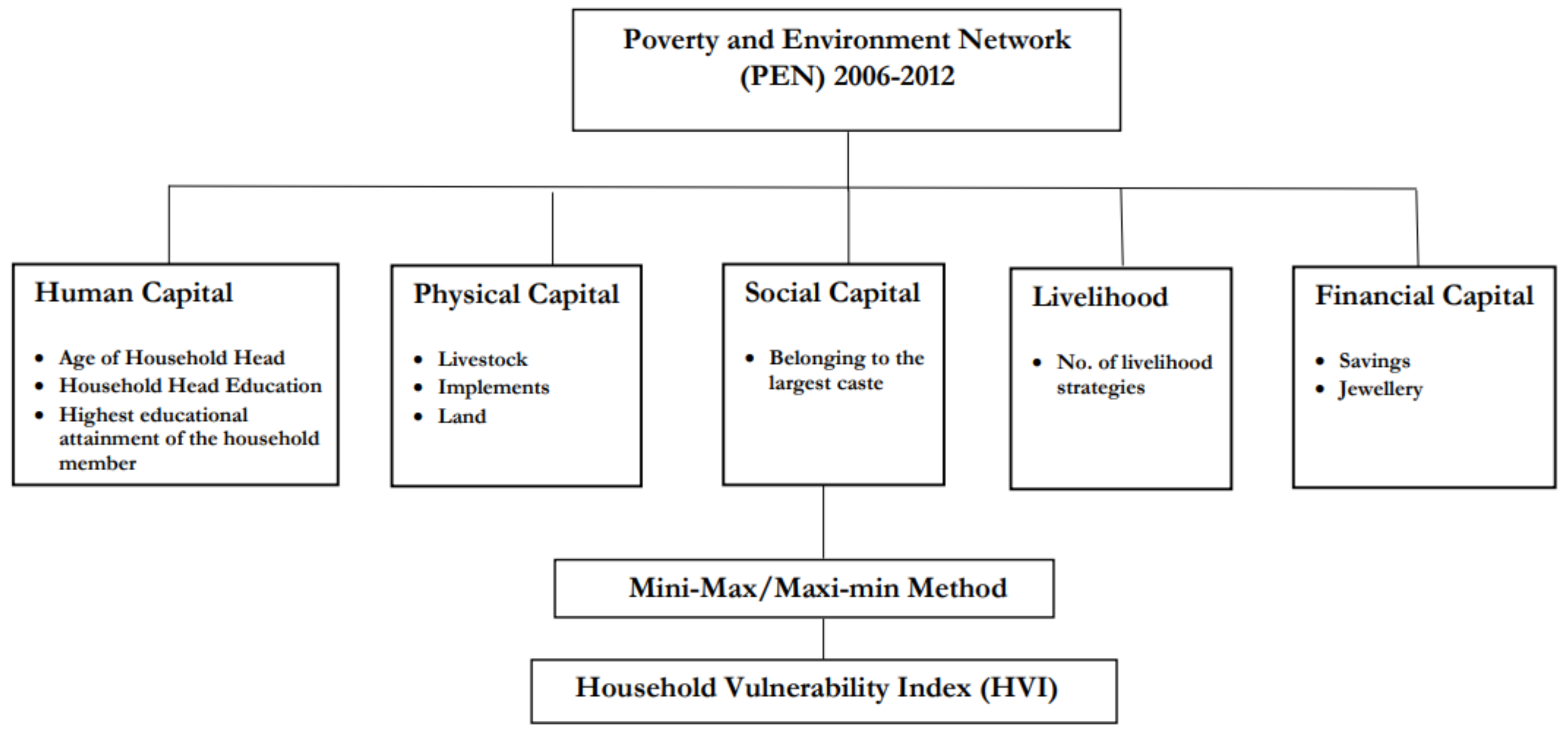
2.1. Household Vulnerability Index

Vulnerability is a state of insecurity experienced when harmful events occur [22,23,24,25]. Financial, human, natural, physical, and social capitals are key determinants of household vulnerability [26,27]. Less vulnerable households demonstrate resilience through alternative livelihoods and strong social connections [28]. The multidimensional nature of vulnerability includes social, economic, physical, institutional, environmental, and attitudinal factors [29,30].
In Nepal, the Social Vulnerability Index (SoVI) was developed to measure social vulnerability and identified high vulnerability in areas inhabited by ethnic minorities [31]. Similarly, another study [32] used a 3SLS technique to estimate Nepal’s vulnerability to poverty, finding an overall vulnerability rate of 33%. Vulnerability scores were notably higher for ethnic minorities and remote areas. Furthermore, many households are highly sensitive to climate-induced disasters due to socio-economic challenges and food insufficiency [33]. This study constructed a community-level Livelihood Vulnerability Index (LVI) and revealed significant spatial variation in vulnerability at the ward level, which is the lowest administrative unit. At the district level, a multidimensional livelihood vulnerability index found that 96.7% of the population in Khotang district, one of Nepal’s most remote regions, was vulnerable [34].
We constructed a Household Vulnerability Index (HVI) to assess varying levels of household vulnerability. A detailed conceptual framework for HVI construction is presented in Figure A1. This index evaluates a household’s possession of five key components: human, physical, social, and financial capitals, and livelihood strategies. Sources of these variables are detailed in Table A6, where a matrix explains their relationship with HVI, references supporting their inclusion from the literature, and their expected influence (positive or negative) on household vulnerability. All indicators were standardized using the method outlined by [35] for life expectancy indices. This standardization ensures that all variables are scaled between 0 and 1 for consistent measurement. We applied this widely used Min-Max normalization technique for this process [25,28,36,37,38]. Variables with different scales were normalized using the formula in Equation (1) for those variables with a positive relationship to vulnerability, and Equation (2) for those with a negative relationship.
X ij = X i X Minj X Maxj X Minj
X ij = X Maxj X i X Maxj X Minj
where X is the observed value of the variable related to household i in district j, and X Max and X Min are maximum and minimum values of each variable, respectively. After normalizing all variables, we used Equation (3) to calculate the final normalized index for each key component.
HVI Cij = 1 n i = 1 n X ij
The HVI Cij is one of the five key components for HH. The main elements include human capital (C1), physical capital (C2), social capital (C3), livelihood (C4), and financial capital (C5). We used Equation (4) to calculate the overall HVI for the HH.
HVI ij = i = 1 n HVI Cij
The HVI serves as a multi-dimensional composite measure of household vulnerability. Each component reflects a critical aspect of household resilience, with equal weights [29,31] ensuring the appropriate balance among components. We assign equal weights and follow an additive approach, which provides a comprehensive framework for identifying and addressing household vulnerability.

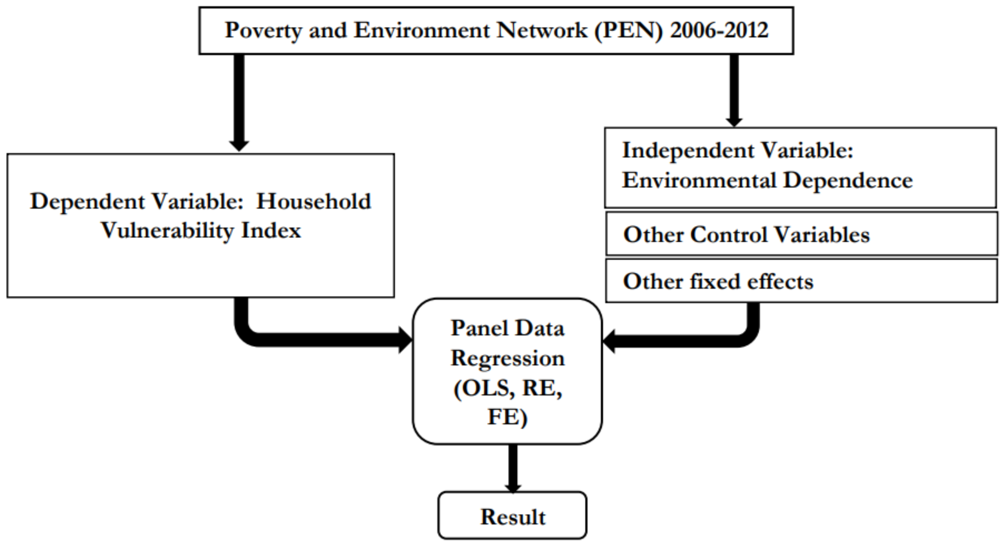
2.2. Household Vulnerability and Environmental Dependence

After constructing the vulnerability index, we analyze the factors that potentially contribute to household vulnerability, focusing on those that may act as liabilities. The sources of these factors are presented in Table A7, where a matrix details their relationship with HVI, relevant literature references, and their expected effect on household vulnerability. Environmental income, while a crucial resource for rural households with limited assets, also presents significant risks, particularly in the face of climate change and environmental degradation. The detailed conceptual framework for this econometric model is presented in Figure A2.
To examine the role of environmental dependence in shaping household vulnerability, we estimate Equation (5) using pooled OLS and panel regression approaches.
HVI i , t = β 0 + δ ED i , t + X i , t β + Z i λ + T t δ t + ϵ
where HVI i , t is the household vulnerability of ith household in t year, ED i , t is environmental dependence, T is the year control variable, X i , t represents the variables controlled for, which include dependency ratio, log of debt, and count of shock experienced, Z i , t represents the control for time invariant fixed effects, such as district and VDCs, and β 0 , δ , β , λ , δ t are the parameters of the model.
We conducted an Individual Effects Test to evaluate the significance of individual-specific effects in the model, along with a Time Fixed Effects Test to assess the presence of time-specific effects. To determine whether a random-effects or fixed-effects model was more appropriate for the data, we applied the Breusch–Pagan Lagrange Multiplier (BPLM) test and the Hausman specification test (details in Appendix B and Table A1).

2.3. Sources of Data and Variables Used

We utilized the environmental income augmented household-level panel dataset [39], which provides representative information on rural livelihoods in Nepal. The survey is geographically representative, encompassing three central physiographic regions of Nepal: Chitwan (lowlands), Kaski (mid-hills), and Mustang (mountains), as shown in Figure 1. A total of 507, 446, and 428 randomly sampled households were surveyed in 2006, 2009, and 2012, respectively. For details on the questionnaire, refer to [40].
The data were collected through the Community Based Forest Management in the Himalaya (ComForM) phases I–III collaborative project conducted by the Institute of Forestry (IOF) at Tribhuvan University and the Department of Food and Resource Economics (IFRO) at the University of Copenhagen, with support from the Department of Forest Research and Survey (DFRS) at the Ministry of Forests and Soil Conservation, Nepal [39,40].
The variables available in the survey, which we used to construct the Household Vulnerability Index (HVI), are summarized in Table 1. Variables were selected based on data availability, scaling characteristics, and relevance as identified in the existing literature, ensuring suitability for calculating household vulnerability. Details on the descriptive statistics of the variables are in Table A2 of Appendix B.4.
The variables used to construct the Household Vulnerability Index (HVI) capture multiple dimensions of household well-being and vulnerability, reflecting rural Nepal’s socio-economic and livelihood context. The age and level of education of the head of the household, together with the highest educational attainment within the household, are key indicators of human capital, directly influencing prosperity and resilience. Physical assets, such as the monetary value of durable goods (e.g., vehicles, equipment, and others) and livestock, are critical components of household wealth and are linked to vulnerability. Land ownership, a cornerstone of Nepali society, is both a productive asset and a store of value, making it a vital inclusion in the index. Financial assets, including savings in banks and jewelry as nonproductive but valuable assets, further capture economic stability. Social capital, represented by membership of castes within the community, recognizes the sociocultural dimensions of vulnerability in Nepal. Lastly, the number of livelihoods a household pursues reflects economic diversification, a critical factor in determining resilience. These variables comprehensively address the determinants of vulnerability and livelihoods in rural Nepal.
Household vulnerability is related to environmental dependence, family dependency, debt, and shock exposure. High dependence on the environment, measured as the ratio of environmental income to total income, suggests a more significant exposure to environmental risks. A higher dependency ratio, which includes children under 15 and seniors over 60, can worsen vulnerability. Additionally, outstanding household debt and the occurrence of financial or natural shocks contribute to vulnerability. While the survey provides detailed data on these key factors, other potential determinants are not included due to data constraints. The measurement and scaling of these variables are summarized in Table 2.

3. Results and Discussion

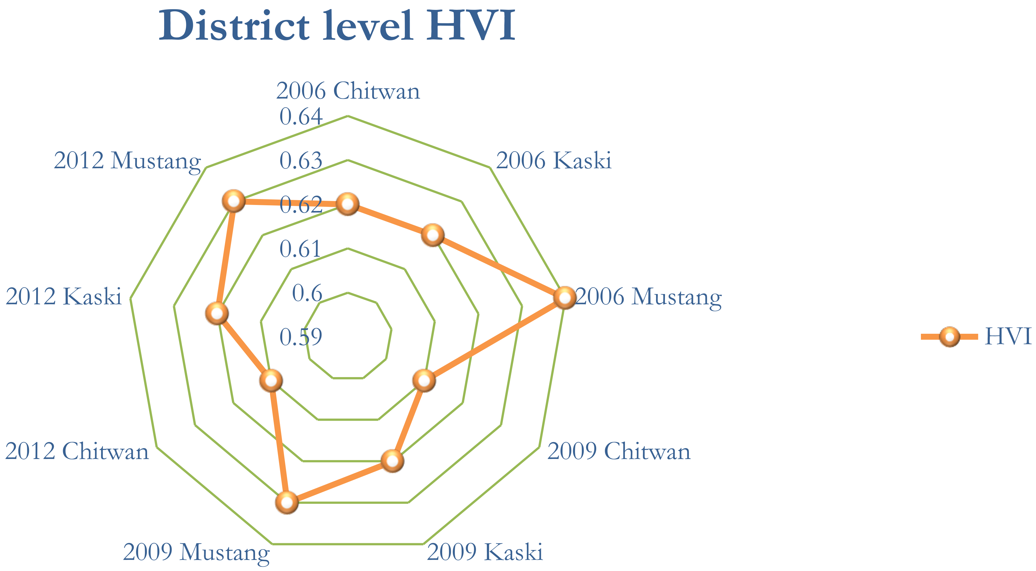
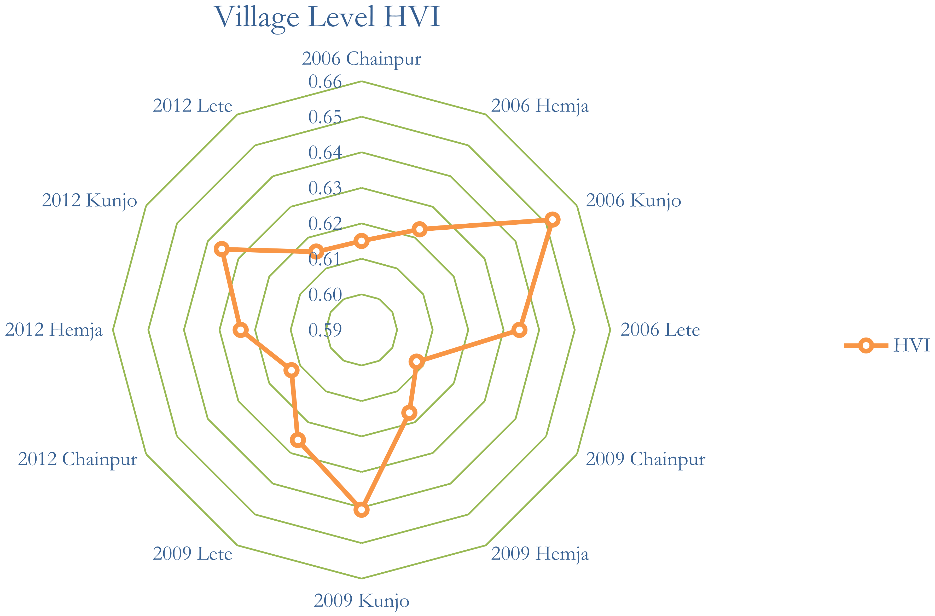
3.1. Nature of the Household Vulnerability

We have calculated the HVI index and summarized its statistical characteristics in Table 3, including the descriptive statistics of the independent variables under consideration. The table is organized into three sections, each corresponding to 2006, 2009, and 2012. It provides statistics for three districts—Chitwan, Kaski, and Mustang—representing different ecological zones of Nepal. Two villages represent Mustang, while Chitwan and Kaski are represented by one village each, with all four villages reported in Table 4 hereunder and Table A3 in Appendix B.4.
In 2006, the mean HVI values for Chitwan, Kaski, and Mustang were 0.62, 0.62, and 0.64, respectively. Similarly, in 2009, the mean HVI values for these districts were 0.61, 0.62, and 0.63, respectively. This trend continued in 2012, with mean HVI values remaining the same in all the respective districts. Since Mustang district includes two sample villages, while Chitwan and Kaski have one village each, the HVI for village-level disaggregated estimations does not differ significantly from the district-level values (Table A3 in Appendix B.4).
The variability in HVI among the sample districts exhibits distinct characteristics, as detailed in Figure A3 and Figure A4 in Appendix B.4. The radar chart for Chainpur shows a polygon with points relatively close to each other, indicating a stable pattern in HVI over the years. The HVI for Chainpur was 0.62 in the first wave of the survey, declined to 0.61 in the second wave, and remained stable through the third wave. Similarly, Hemja’s radar chart indicates a consistent HVI across all survey waves, remaining at 0.62 throughout.
The mean HVI for Kaski district remained stable across all three rounds. However, the standard deviation slightly increased in the third round. Kaski, including the sample village, relies heavily on remittances and tourism and is more urbanized than Chitwan and Mustang. This economic dependence on resilient sectors may explain the stability in vulnerability levels. The rising standard deviation of the HVI could indicate greater variability, as improvements in human capital, financial capital, and physical capital disproportionately benefit certain households.
The vulnerability levels in Chitwan and Mustang showed improvement in the second survey round compared to the first, but remained unchanged in the final round. The formal resolution of the political conflict during this period positively influenced the determinants of HVI. Both Chitwan and Mustang, with economies centered on tourism and agriculture, likely experienced a direct relationship between political and governance stability and reductions in household vulnerability.
One of the sample villages from Mustang, Kunjo, was found to be the most vulnerable area. The HVI index showed no improvement across all three survey rounds, with only a slight increase in standard deviation in the second round. In contrast, the average HVI in another sample village, Lete, also from Mustang, improved in both the second and third rounds. This variation between the villages is likely due to their distance from the district headquarters, with more remote villages relying on traditional subsistence-based economic activities, while those closer to the district center are more dependent on tourism, trade, and other service sectors. The average of these sample villages represents Mustang district in our analysis, and the HVI data for the district follows a pattern similar to Chitwan, where vulnerability slightly improved in the second round and remained stable in the third.

3.2. Environmental Dependence and Vulnerability

We regressed the vulnerability of the household (HVI) to environmental dependence, the ratio of dependent family members, household debt, and the shocks experienced by the household. The results showed that a higher share of income from the natural environment, representing environmental dependence, tends to increase the vulnerability of a household. In contrast, household debt reduces vulnerability. However, shocks experienced by households are positively linked to increased vulnerability. We also control for time, district, and VDC variables in subsequent estimations. The summary of the regression results is in Table 5 for pooled OLS, and in Table 6 for random effect panel estimates. We have retained the regression results for fixed effect panel regression in Table A5 in Appendix B.4 for reference.
We estimated the pooled OLS regression of household vulnerability, initially including only environmental dependence, and the results of the regression (1) are presented in Table 5. The coefficient is statistically significant and positive, indicating that households with higher environmental dependence would be vulnerable, assuming other factors remain constant. While the regression appears acceptable, the coefficient of determination is relatively low, as expected, given the limited number of explanatory variables included.
We stepwise added dependency ratio, household debt, and shocks in the estimates; the data availability permitted us up to these four explanatory variables, including district and village control only. The coefficient for environmental dependency in all models remained consistent in magnitude and direction both. All four coefficients are significant statistically; the coefficient of determination gradually improves as expected (see regressions (2)–(4) in Table 6).
We performed an LM test to evaluate the null hypothesis of no statistically significant time effects in the model, following the method outlined by [41]. The results strongly rejected the null hypothesis, providing evidence of time effects. Details of the test are provided in Table A1, Appendix B.4. Consequently, we included time (year) and time-invariant factors (district and VDC) in the model. The findings confirm the presence of both time and individual effects, prompting us to control for year, district, and VDC fixed effects.
To assess the poolability of the data, we conducted the BP-LM test [42], which evaluates whether the cross-sectional units in the panel share statistically identical intercepts and slopes. The results, detailed in Table A1 in Appendix B.4, indicate that for models (1)–(3), the panel data are not poolable.
The regression results for models (1)–(3) show minimal changes in magnitude and direction across the pooled, random effects, and fixed effects estimations. However, our findings and interpretations are primarily based on models (4)–(7), as these models incorporate all possible controls sequentially. These models also explain a higher proportion of the variation in the dependent variable compared to others. The Hausman specification test further suggests using random effects models for models (4)–(7) throughout, as detailed in Table A1. Accordingly, we report the pooled regression summary in Table 5, the random effects summary in Table 6, and the fixed effects results in Table A5 in Appendix B.4.
The Random Effects panel regression estimations of household vulnerability are summarized in Table 6. The environmental dependence coefficients in all seven alternative estimations are positive and statistically significant at the 1% level. This is our primary explanatory variable, confirming a positive and significant association between the share of environmental income and HVI, ceteris paribus.
We interpret the coefficients from the seventh model in Table 6 as a representative model and the best among several. A one-unit increase in environmental dependence is associated with a 0.141-unit increase in household vulnerability in rural Nepal, holding other factors constant. An increase of one unit in the ratio of dependents to working family members corresponds to a 0.009-unit rise in vulnerability, ceteris paribus. Households experiencing shock tend to exhibit higher vulnerability; however, this coefficient is not statistically significant. Contrary to the positive contributors above, a one-unit increase in the share of debt relative to household income leads to a 0.004-unit decrease in vulnerability, assuming all other variables remain constant.
The share of dependent elderly and young family members relative to working-age members is another explanatory variable in our analysis. The regression coefficients across models (2)–(7) are consistently positive and statistically significant at the 1% level. When a household has more dependent members, two challenges may arise. First, resources are shared among more individuals. Second, there is less contribution to household income, as the working members’ time may be diverted from income-generating activities to caregiving. The imperfect social security system and reliance on manual and primitive livelihood activities likely demand longer working hours. Consequently, in addition to environmental dependence, increased family responsibilities and household chores may push rural households into greater vulnerability.
Another explanatory variable in our estimates is household-level debt. The coefficient is negative and statistically significant across models (4)–(7), even at the 1% to 10% significance levels. This indicates that households with debt are less vulnerable. It is possible that these households have taken on debt as a coping mechanism to address vulnerabilities. Additionally, it is plausible that households with the capacity to borrow, supported by formal or informal collateral at the local level, are relatively better off, making them less vulnerable despite being indebted. The regression coefficients for the variable representing shocks, defined as the number of types of shocks a household faced, are consistently positive in models (3)–(7), though not statistically significant throughout. The shocks experienced by households are indeed related to vulnerability. However, when we control for year, district, and VDC, the coefficient slightly decreases, suggesting that these controls may partially account for the effects of such shocks.

3.3. Discussion

The patterns of household vulnerability across districts observed in previous studies highlight how geography, economic activities, and social factors shape vulnerability dynamics. In Kaski, the stable and relatively low vulnerability can be attributed to its peri-urban characteristics and better socio-economic status of areas like Hemja. Studies have shown that peri-urban areas often benefit from access to urban resources, infrastructure, and diversified livelihoods, reducing the reliance on subsistence-level environmental income [43]. This is consistent with research suggesting that urban proximity often contributes to enhanced economic resilience [44], similar to Kaski district in our case.
In contrast, the fluctuations observed in Chitwan and Mustang reflect broader patterns seen in rural regions with distinct geographic and economic features. The reduction in vulnerability in Chitwan aligns with its location in the lowland Tarai, where agricultural productivity and economic opportunities have historically been higher. The Tarai’s fertile land and infrastructure development have long been associated with more stable livelihoods, as noted in studies on agricultural-based resilience [45]. Mustang, however, demonstrates the unique vulnerability of high-altitude, remote areas, where environmental and socio-economic challenges exacerbate vulnerability before stabilizing due to the gradual development of coping mechanisms. This aligns with findings from rural development studies highlighting that remote areas with limited access to resources and markets face higher initial vulnerability but may stabilize as adaptive strategies evolve over time [46].
These district-level patterns reflect broader trends in rural vulnerability across different geographical contexts. It is revealed that the vulnerability varies based on environmental, socio-economic, and geographical factors, urging further investigation into the specific drivers of vulnerability [47,48]. In particular, the case of Mustang highlights the complexity of vulnerability in mountainous and remote areas, where initial high vulnerability may not necessarily reflect a permanent condition but could instead indicate transitional phases in coping strategies. These findings suggest that further research is needed to better understand whether such fluctuations in vulnerability signify long-term resilience or temporary adjustments, as highlighted in resilience and vulnerability studies [49].
The regression results offer valuable insights into household vulnerability. Environmental dependence emerges as a significant factor contributing to greater household vulnerability, holding other factors constant. This finding superseded previous beliefs in Nepal, where environmental dependence is high due to extensive protected areas and celebrated community-based forest conservation practices. While community forestry and environmental stewardship are often lauded for their role in poverty reduction and development, heavy reliance may exacerbate vulnerability. Ref. [8] rightly points out the dual role of environmental income: it can act as a safety net for rural livelihoods by buffering poverty, but also exposes households to ecological shocks. The environmental dependence might empower local populations, but could impose precarity regarding access and equity, potentially intensifying household-level vulnerability [50]. Over-reliance on natural resources heightens exposure to environmental risks, undermining long-term resilience [51]. These insights suggest that while environmental resources offer immediate benefits, their over-dependence can exacerbate precarity, particularly in rural economies like Nepal, where ecological and socio-political factors intersect.
Household debt, as a coping mechanism, shows a negative but statistically insignificant relationship with vulnerability. Debt provides financial support during shocks, acting as a safety net and enhancing resilience by enabling households to smooth consumption and mitigate the effects of shocks [52]. In addition, debt can facilitate investment in productive activities, which reduces vulnerability and fosters long-term resilience. Access to borrowing plays a crucial role in managing risk and improving household resilience, particularly in rural economies [53]. Furthermore, households with access to credit—whether from formal or informal sources—often possess physical and social capital, which strengthens their capacity to withstand vulnerabilities. These insights highlight the importance of credit access in enhancing household resilience, despite its statistically insignificant direct effect in the present study. Contemporary studies further support the idea that debt serves as a key coping mechanism during emergencies. For instance, during the COVID-19 pandemic, debt played a vital role in managing economic shocks in Indonesia [54], while environmental factors influenced borrowing behaviors and financial resilience in rural India [55].
A high dependency ratio, with more dependents relative to working-age members, increases household vulnerability by heightening susceptibility to economic shocks and financial instability. Caregiving responsibilities for older people and children often require adults to forgo income-generating opportunities, further exacerbating vulnerability. The literature suggests that caregiving can lead to welfare loss and negatively affect mental health [56], while high dependency ratios place additional economic pressures on households, making it harder to cope with financial challenges [57].
Households in rural Nepal are highly vulnerable to various shocks, such as natural disasters, economic downturns, health shocks, and both idiosyncratic and covariate shocks, severely impacting their livelihoods. These shocks tend to exacerbate pre-existing vulnerabilities, disproportionately affecting the poor and marginalized. Research confirms that households experiencing at least one shock are more susceptible to long-term consequences than those without such exposure. While households can typically withstand minor shocks, larger ones pose significant risks to assets, food security, and overall welfare, with the effects lasting up to two years [58]. Similarly, combining the 2015 earthquake and subsequent monsoon anomalies significantly worsened food insecurity, particularly in steep, mountainous areas [59].

4. Conclusions and Recommendations

This study highlights key patterns of household vulnerability in rural Nepal. Kaski demonstrates stable and low vulnerability, likely due to its peri-urban setting and reliance on service sectors like tourism and remittances. In contrast, Chitwan and Mustang show initial declines in vulnerability followed by stabilization, driven by factors such as agricultural productivity, governance, and adaptation strategies. Thus, socioeconomic-ecological dimensions are essential in analyzing the vulnerability of rural households in Nepal. The results confirm that environmental dependence significantly increases household vulnerability, emphasizing the risks associated with reliance on natural resources. Household debt mitigates vulnerability by providing financial support and enabling productive investments. However, a high dependency ratio exacerbates vulnerability by limiting income generation due to caregiving demands. Shocks, while not always statistically significant, consistently correlate with increased vulnerability, highlighting their destabilizing effects on rural households.
There is scope to reduce environmental dependence by promoting diversification in economic activities and strengthening social safety nets to build resilience. Sustainable livelihood programs and rural economic development initiatives could help decrease reliance on natural resources. In Nepal, significant power has been devolved to local governments, with three tiers of governance proving effective in recent years. The transparent distribution of royalties and subsidies, coupled with the ability of local governments to operate at the community level, offers unique opportunities. Local government-led interventions in education, healthcare, and income generation could significantly enhance household resilience against vulnerability. Expanding access to credit and promoting responsible borrowing practices may prevent financial instability, and Nepal has unique experiences of social mobilization and community-level self-help groups. Establishing childcare and eldercare facilities could alleviate caregiving burdens on households with high dependency ratios. Investments in disaster preparedness, risk reduction measures, and resilient infrastructure will also be crucial for mitigating vulnerability.
Future research could explore the intersection of resilience and vulnerability, incorporating comprehensive primary data on environmental dependence. Integrating such data with nationally representative surveys and census information could offer a clearer national-level perspective. Including disaster-related data, potentially enhanced by remote sensing, would add valuable depth. Employing causal analysis and extensive datasets could refine policy recommendations and strengthen resilience-building strategies. Additionally, examining the political and economic dimensions, particularly the role of local governments and governance quality, may provide critical insights.

Author Contributions

Conceptualization, R.T.-P.; Methodology, R.T.-P. and S.N.; Software, S.N.; Validation, R.P.; Formal analysis, R.T.-P. and S.N.; Data curation, S.N., B.K. and R.P.; Writing—original draft, S.N.; Writing—review & editing, R.T.-P. and B.K.; Visualization, B.K. and R.P.; Supervision, R.T.-P.; Project administration, S.N. All authors have read and agreed to the published version of the manuscript.

Funding

This research was partially funded by the Research Directorate, Rector’s Office, Tribhuvan University, Nepal, with S.N. receiving the Master’s Thesis Grant (EF-80-81-491) for this work.

Institutional Review Board Statement

Not applicable.

Informed Consent Statement

Not applicable.

Data Availability Statement

The data presented in this study are available on request from the corresponding author.

Conflicts of Interest

The funders had no role in the design of the study; in the collection, analyses, or interpretation of data; in the writing of the manuscript; or in the decision to publish the results.

Appendix A

Figure A1. Conceptual framework for HVI construction.
Sustainability 17 02434 g0a1
Figure A2. Household vulnerability analysis framework.
Sustainability 17 02434 g0a2

Appendix B. Diagnostic Test Results

Appendix B.1. Lagrange Multiplier Test-(Honda) Time Effects Test

data: HVI ∼ Environmental Dependency + Debt + Dependency ratio + Shock + … n o r m a l = 10.822 , p-value < 2.2 × 10 16
alternative hypothesis: significant effects

Appendix B.2. F Test for Individual Effects

data: HVI ∼ Environmental Dependency + Debt + Dependency ratio + shock+… F = 2.4874 , d f 1 = 427 , d f 2 = 852 , p-value < 2.2 × 10 16
alternative hypothesis: significant effects

Appendix B.3. Lagrange Multiplier Test-(Breusch-Pagan)

data: HVI ∼ Environmental Dependency + Debt + Dependency ratio + shock+… c h i s q = 117.12 , d f = 1 , p-value < 2.2 × 10 16
alternative hypothesis: significant effects

Appendix B.4. Hausman Test

data: HVI ∼ Environmental Dependency + Debt + Dependency ratio + shock+… c h i s q = 25.48 , d f = 6 , p-value = 0.0002782
alternative hypothesis: one model is inconsistent
Table A1. Appendix on Diagnostic test results.
ModelTime FE Test BP-LM Test Hausman Test
Normalp-ValueChi²p-ValueChi²p-Value
116.7312.2 × 10 16 11.2080.00080.99930.3175
216.7412.2 × 10 16 11.1410.00080.99380.6084
316.8282.2 × 10 16 7.6700.00564.47540.2145
416.8642.2 × 10 16 0.2770.59893.84500.4274
517.0812.2 × 10 16 1.5040.22018.4915 × 10 12 1.0000
614.9162.2 × 10 16 1.5040.22017.8704 × 10 12 1.0000
714.9302.2 × 10 16 1.5040.22013.2437 × 10 11 1.0000
Figure A3. District-level HVI for all waves.
Sustainability 17 02434 g0a3
Figure A4. Village-level HVI for all waves.
Sustainability 17 02434 g0a4
Table A2. Mean and SD variables used to construct the vulnerability index.
Year200620092012
DistrictChitwanKaskiMustangChitwanKaskiMustangChitwanKaskiMustang
Human Capital
hhh_age50.36
(14.15)
50.14
(14.57)
52.89
(13.52)
52.13
(13.75)
52.00
(13.39)
54.12
(13.78)
52.24
(17.20)
53.52
(13.71)
55.24
(14.17)
hhh_edu3.08
(4.06)
6.29
(4.97)
3.05
(3.98)
2.93
(4.06)
6.07
(5.23)
2.94
(3.78)
2.91
(4.33)
6.91
(5.07)
2.90
(4.08)
max_hh_edu8.44
(3.91)
10.76
(2.90)
7.64
(3.32)
9.70
(3.63)
11.18
(3.94)
8.04
(3.93)
9.89
(4.44)
11.91
(4.03)
8.22
(3.87)
Physical Capital
implements4660.32
(11,275.51)
14,057.03
(16,860.40)
10,360.32
(19,629.35)
10,153.80
(23,970.96)
30,700.04
(46,128.42)
15,135.16
(25,508.99)
22,165.29
(38,089.26)
48,959.03
(70,582.61)
21,466.58
(27,566.06)
livestock18,532.68
(15,428.31)
26,573.08
(20,411.58)
80,387.77
(224,589.10)
43,936.83
(39,679.86)
35,690.11
(35,760.04)
56,165.26
(178,639.73)
38,993.71
(34,330.39)
34,635.85
(39,306.64)
34,114.52
(39,335.73)
land2027.47
(6367.27)
1187.00
(1013.02)
2940.39
(2789.36)
915.91
(765.38)
1491.41
(2060.26)
2235.09
(3738.40)
1041.46
(1136.88)
1374.96
(2253.95)
1921.22
(1892.77)
Social Capital
hh_caste0.58
(0.50)
0.89
(0.32)
0.49
(0.50)
0.66
(0.48)
0.98
(0.14)
0.58
(0.50)
0.50
(0.50)
0.86
(0.50)
0.59
(0.42)
Financial Capital
bank_saving879.58
(2661.50)
9663.83
(26,812.59)
31,897.65
(79,933.66 )
1911.63
(6126.69)
11,937.72
(31,025.90)
24,536.06
(59,338.85)
11,953.55
(31,763.88)
25,410.64
(66,932.36)
48,051.24
(104,495.00)
jewellery0.00
(0.00)
0.00
(0.00)
31,662.91
(67,846.57)
4396.88
(6965.54)
20,485.87
(16,594.27)
38,598.35
(79,440.96)
21,477.20
(23,620.48)
51,605.95
(48,463.66)
54,132.35
(112,328.06)
Livelihood
n_livelihoods4.81
(0.97)
4.72
(0.91)
4.56
(0.93)
4.93
(1.02)
4.74
(0.91)
5.11
(0.84)
4.60
(0.98)
4.78
(0.90)
4.60
(0.98)
Household Vulnerability
HVI0.61
(0.05)
0.62
(0.04)
0.64
(0.05)
0.61
(0.05)
0.62
(0.04)
0.63
(0.05)
0.61
(0.05)
0.62
(0.05)
0.63
(0.05)
Note: SD in the parentheses. Source: author’s calculation.
Table A3. Village-level mean and SD HVI for all waves.
Year/
District
200620092012
ChainpurHemjaKunjoLeteChainpurHemjaKunjoLeteChainpurHemjaKunjoLete
HVI0.62
(0.05)
0.62
(0.04)
0.65
(0.04)
0.63
(0.05)
0.61
(0.05)
0.62
(0.04)
0.64
(0.04)
0.63
(0.05)
0.61
(0.05)
0.62
(0.05)
0.64
(0.05)
0.62
(0.05)
Note: Standard deviation in the parentheses; Source: author’s calculation.
Table A4. Panel data regression.
Dependent Variable: Household Vulnerability
(1)(2)(3)(4)
Env. Dependence0.108 ***0.141 ***0.141 ***0.141 ***
(0.013)(0.014)(0.014)(0.014)
Dependency ratio 0.009 ***0.009 ***0.009 ***
(0.003)(0.003)(0.003)
Shock 0.00020.00020.0002
(0.004)(0.004)(0.004)
Debt −0.004 **−0.004 **−0.004 **
(0.002)(0.002)(0.002)
Constant0.683 ***0.694 ***0.694 ***
(0.007)(0.008)(0.008)
Year-fixed effectsNoYesYesYes
District-fixed effectsNoYesYesYes
VDC-fixed effectsYesYesYesYes
Observations1245124512451245
R 2 0.0490.1830.1830.174
Adjusted R 2 0.0480.1770.1770.168
Statistical significance indicators: ** p < 0.05, *** p < 0.01; Env. = Environmental.
Table A5. Fixed effects regression.
Dependent Variable: Household Vulnerability
(1)(2)(3)(4)(5)(6)(7)
Env. Dependence0.106 ***0.104 ***0.103 ***0.128 ***0.131 ***0.131 ***0.140 ***
(0.014)(0.014)(0.014)(0.014)(0.014)(0.014)(0.014)
Dependency ratio 0.009 ***0.009 ***0.008 **0.008 **0.008 **0.009 ***
(0.003)(0.003)(0.003)(0.003)(0.003)(0.003)
Shock 0.0050.0050.0050.0050.0002
(0.004)(0.004)(0.004)(0.004)(0.004)
Debt −0.006 ***−0.004 *−0.004 *−0.004 **
(0.001)(0.002)(0.002)(0.002)
Year-fixed effectsNoNoNoNoYesYesYes
District-fixed effectsNoNoNoNoNoYesYes
VDC-fixed effectsNoNoNoNoNoNoYes
Observations1245124512451245124512451245
R 2 0.0470.0530.0540.0750.0760.0760.174
Adjusted R 2 0.0440.0500.0500.0710.0710.0710.168
Statistical significance indicators: * p < 0.1, ** p < 0.05, *** p < 0.01; Env. = Environmental.
Table A6. Household vulnerability index construction and metrics.
VariableDescriptionExpected Sign (+/−)
HH head’s educational attainmentHH head’s educational attainment enhances access to information, improves decision-making, and increases income opportunities, enabling better risk management and resilience, thereby reducing household vulnerability [27,29,60,61].Higher educational level (−)
Highest educational attainment by an HH memberFamily members with higher education levels contribute to increased HH income, improved access to resources and better adaptive capacity, thereby reducing overall household vulnerability [28,29,37].Maximum (−)
Implements ValueThe total value of implements (Cars, Trucks, Motorbike, Plough, etc.) reflects household assets that enhance mobility, productivity, and income opportunities, reducing vulnerability by improving resilience and market access [27,61].Higher Value (−)
Livestock ValueTotal value of livestock (all types) in Rs. serves as a key household asset, providing income, food security, and a financial safety net, thereby reducing vulnerability and enhancing resilience [28,60].Higher Value (−)
Land areaThe total area of land owned by the household (sq. m) represents a crucial asset that supports livelihood, food security, and income generation, enhancing economic stability and reducing vulnerability [28,61].Greater land area (−)
HH CasteHouseholds belonging to the largest caste in the village (=1) indicate social positioning and access to community resources, networks, and opportunities, potentially reducing vulnerability through social capital and support systems [28,62].Largest caste (−)
Bank savingHousehold savings in banks or recognized financial institutions enhance financial security, facilitate access to credit, and improve resilience to economic shocks, reducing household vulnerability [63].Greater saving (−)
JewelleryHousehold savings in the form of non-productive assets serve as a financial reserve, providing liquidity during emergencies, but with limited income-generating potential compared to productive assets [64].Greater value (−)
LivelihoodThe count of livelihoods of the household represents the household’s economic diversification. A higher number of income sources enhances financial stability, reduces dependency on a single sector, and improves resilience to economic shocks, thereby lowering vulnerability [28,37].Diversified (−)
Table A7. Household vulnerability and environmental dependence.
VariableDescriptionExpected Sign (+/−)
Environmental DependenceThe ratio of Environmental Income to Total Income of the Household Reflects a household’s reliance on natural resources for livelihood. Higher environmental dependence is expected to increase household vulnerability, as it indicates greater exposure to environmental risks, resource depletion, and economic instability, making households more susceptible to shocks [8,65].Greater dependence (+)
Dependency RatioRatio of Dependent to Working Adult Members of the Household Represents the economic burden on working members. A higher dependency ratio increases household vulnerability by straining resources, limiting savings, and reducing the household’s ability to cope with financial shocks [29,34,66,67].Higher ratio (−)
DebtTotal Household Debt (Rs.) Indicates financial obligations that may constrain household resources. Higher debt levels increase vulnerability by reducing disposable income, limiting investment in productive assets, and heightening financial stress during economic shocks [68].Higher value of debt (−)
ShockIndicates whether the household has faced adverse events. Experiencing shocks increases vulnerability by disrupting income, depleting assets, and weakening the household’s ability to recover and build resilience [61,69,70].Experienced shock (+)

References

  1. Jaszczak, A.; Kristianova, K.; Vaznonienė, G.; Žukovskis, J. Phenomenon of abandoned villages and its impact on transformation of rural landscapes. Manag. Theory Stud. Rural. Bus. Infrastruct. Dev. 2018, 40, 467–480. [Google Scholar] [CrossRef]
  2. World Bank. Rural Population (% of Total Population). 2021. Available online: https://data.worldbank.org/indicator/SP.RUR.TOTL.ZS (accessed on 4 February 2025).
  3. United Nations. World Urbanization Prospects 2018. 2018. Available online: https://population.un.org/wup (accessed on 4 February 2025).
  4. Acharya, B.R. Dimension of rural development in Nepal. Dhaulagiri J. Sociol. Anthropol. 2008, 2, 181–192. [Google Scholar] [CrossRef]
  5. FAO; IFAD; UNICEF; WFP; WHO. The State of Food Security and Nutrition in the World 2021: Transforming Food Systems for Food Security, Improved Nutrition and Affordable Healthy Diets for All; FAO: Rome, Italy, 2021. [Google Scholar]
  6. Gemenne, F. The Impacts of Migration for Adaptation and Vulnerability. 2022. Available online: https://www.delmi.se/media/l4acp0cq/delmi-research-overview-2022_2-webb.pdf (accessed on 4 February 2025).
  7. Pelser, A.J.; Chimukuche, R.S. Climate Change, Rural Livelihoods, and Human Well-Being: Experiences from Kenya. In Vegetation Dynamics, Changing Ecosystems and Human Responsibility; IntechOpen: London, UK, 2022. [Google Scholar] [CrossRef]
  8. Angelsen, A.; Jagger, P.; Babigumira, R.; Belcher, B.; Hogarth, N.J.; Bauch, S.; Börner, J.; Smith-Hall, C.; Wunder, S. Environmental income and rural livelihoods: A global-comparative analysis. World Dev. 2014, 64, S12–S28. [Google Scholar] [CrossRef]
  9. United Nations. Rural Population Left Behind by Uneven Global Economy. 2019. Available online: https://press.un.org/en/2019/gaef3521.doc.htm (accessed on 4 February 2025).
  10. Lazarte-Hoyle, A. Understanding the Drivers of Rural Vulnerability Towards Building Resilience, Promoting Socio-Economic Empowerment and Enhancing the Socio-Economic Inclusion of Vulnerable, Disadvantaged and Marginalized Populations for an Effective Promotion of Decent Work in Rural Economies; International Labour Organization: Geneva, Switzerland, 2017. [Google Scholar]
  11. McNamara, K.E.; Olson, L.L.; Rahman, M.A. Insecure hope: The challenges faced by urban slum dwellers in Bhola Slum, Bangladesh. Migr. Dev. 2016, 5, 1–15. [Google Scholar] [CrossRef]
  12. Tacoli, C.; Mcgranahan, G. Urbanisation, Rural-Urban Migration and Urban Poverty; Human Settlements Group, International Institute for Environment and Development: London, UK, 2015. [Google Scholar]
  13. Artuso, M. State of the World’s Cities 2010/11–Bridging the Urban Divide, by UN Habitat; Earthscan: London, UK, 2011; ISBN 978-1-84971-176-0. [Google Scholar]
  14. Nawrotzki, R.; Hunter, L.; Dickinson, T.W. Natural resources and rural livelihoods: Differences between migrants and non-migrants in Madagascar. Demogr. Res. 2012, 26, 661–700. [Google Scholar] [CrossRef]
  15. Angelsen, A.; Wunder, S. Exploring the forest-poverty link. CIFOR Occas. Pap. 2003, 40, 1–20. [Google Scholar]
  16. Emeru, G.M.; Fikire, A.H.; Beza, Z.B. Determinants of urban households’ livelihood diversification strategies in North Shewa Zone, Ethiopia. Cogent Econ. Financ. 2022, 10, 2093431. [Google Scholar] [CrossRef]
  17. Amevenku, F.; Asravor, R.; Kuwornu, J.K. Determinants of livelihood strategies of fishing households in the volta Basin, Ghana. Cogent Econ. Financ. 2019, 7, 1595291. [Google Scholar] [CrossRef]
  18. Chambers, R.; Conway, G. Sustainable Rural Livelihoods: Practical Concepts for the 21st Century; Institute of Development Studies: Falmer, UK, 1992. [Google Scholar]
  19. DfID. Sustainable Livelihoods Guidance Sheets; DFID: London, UK, 1999; Volume 445, p. 710. [Google Scholar]
  20. Ellis, F. Rural Livelihood Diversity in Developing Countries: Evidence and Policy Implications. In Natural Resource Perspectives; Overseas Development Institute: London, UK, 1999; Volume 40, pp. 1–10. [Google Scholar]
  21. Scoones, I. Livelihoods perspectives and rural development. In Critical Perspectives in Rural Development Studies; Routledge: London, UK, 2013; pp. 159–184. [Google Scholar]
  22. Chambers, R. Editorial introduction: Vulnerability, coping and policy. IDS Bull. 1989, 20, 1–7. [Google Scholar] [CrossRef]
  23. Calvo, C.; Dercon, S. Measuring Individual Vulnerability; University of Oxford: Oxford, UK, 2005. [Google Scholar]
  24. Chambers, R. Vulnerability, coping and policy (editorial introduction). IDS Bull. 2006, 37, 33–40. [Google Scholar] [CrossRef]
  25. Fang, Y.p.; Zhao, C.; Rasul, G.; Wahid, S.M. Rural household vulnerability and strategies for improvement: An empirical analysis based on time series. Habitat Int. 2016, 53, 254–264. [Google Scholar] [CrossRef]
  26. Gaisie, E.; Han, S.S.; Kim, H.M. Complexity of resilience capacities: Household capitals and resilience outcomes on the disaster cycle in informal settlements. Int. J. Disaster Risk Reduct. 2021, 60, 102292. [Google Scholar] [CrossRef]
  27. Zhang, H.; Zhao, Y.; Pedersen, J. Capital assets framework for analysing household vulnerability during disaster. Disasters 2020, 44, 687–707. [Google Scholar] [CrossRef]
  28. Antwi-Agyei, P.; Dougill, A.J.; Fraser, E.D.; Stringer, L.C. Characterising the nature of household vulnerability to climate variability: Empirical evidence from two regions of Ghana. Environ. Dev. Sustain. 2013, 15, 903–926. [Google Scholar] [CrossRef]
  29. Rahman, M.M.; Arif, M.S.I.; Hossain, M.T.; Almohamad, H.; Al Dughairi, A.A.; Al-Mutiry, M.; Abdo, H.G. Households’ vulnerability assessment: Empirical evidence from cyclone-prone area of Bangladesh. Geosci. Lett. 2023, 10, 26. [Google Scholar] [CrossRef]
  30. Notenbaert, A.; Karanja, S.N.; Herrero, M.; Felisberto, M.; Moyo, S. Derivation of a household-level vulnerability index for empirically testing measures of adaptive capacity and vulnerability. Reg. Environ. Chang. 2013, 13, 459–470. [Google Scholar] [CrossRef]
  31. Aksha, S.K.; Juran, L.; Resler, L.M.; Zhang, Y. An analysis of social vulnerability to natural hazards in Nepal using a modified social vulnerability index. Int. J. Disaster Risk Sci. 2019, 10, 103–116. [Google Scholar] [CrossRef]
  32. Shahi, P.R.; Shreezal, G. Estimating Households’ Vulnerability to Poverty. Econ. J. Nepal 2020, 43, 17–35. [Google Scholar]
  33. Bista, R.B. Grasping Climate Vulnerability in Western Mountainous Nepal: Applying Climate Vulnerability Index. Proc. Forum Soc. Econ. 2019, 50, 553–568. [Google Scholar] [CrossRef]
  34. Gerlitz, J.Y.; Macchi, M.; Brooks, N.; Pandey, R.; Banerjee, S.; Jha, S.K. The multidimensional livelihood vulnerability index–an instrument to measure livelihood vulnerability to change in the Hindu Kush Himalayas. Clim. Dev. 2017, 9, 124–140. [Google Scholar] [CrossRef]
  35. UNDP. Human development report 2007/8. Fighting climate change: Human solidarity in a divided world. In Fighting Climate Change: Human Solidarity in a Divided World (November 27, 2007); UNDP-HDRO Human Development Report; UNDP: New York, NY, USA, 2007. [Google Scholar]
  36. Karunarathne, A.Y.; Lee, G. Developing a multi-facet social vulnerability measure for flood disasters at the micro-level assessment. Int. J. Disaster Risk Reduct. 2020, 49, 101679. [Google Scholar] [CrossRef]
  37. Huynh, L.T.M.; Stringer, L.C. Multi-scale assessment of social vulnerability to climate change: An empirical study in coastal Vietnam. Clim. Risk Manag. 2018, 20, 165–180. [Google Scholar] [CrossRef]
  38. Dumenu, W.K.; Takam Tiamgne, X. Social vulnerability of smallholder farmers to climate change in Zambia: The applicability of social vulnerability index. SN Appl. Sci. 2020, 2, 1–16. [Google Scholar] [CrossRef]
  39. Walelign, S.Z.; Smith-Hall, C.; Rayamajhi, S.; Chhetri, B.B. A unique environmental augmented household-level livelihood panel dataset from Nepal. Data Brief 2022, 42, 108168. [Google Scholar] [CrossRef]
  40. Larsen, H.O.; Rayamajhi, S.; Chhetri, B.B.K.; Charlery, L.C.; Gautam, N.; Khadka, N.; Puri, L.; Rutt, R.L.; Shivakoti, T.; Thorsen, R.S. The role of environmental incomes in rural Nepalese livelihoods 2005–2012: Contextual information. IFRO Doc. 2014, 4. [Google Scholar]
  41. Honda, Y. A size correction to the Lagrange multiplier test for heteroskedasticity. J. Econom. 1988, 38, 375–386. [Google Scholar] [CrossRef]
  42. Breusch, T.S.; Pagan, A.R. The Lagrange multiplier test and its applications to model specification in econometrics. Rev. Econ. Stud. 1980, 47, 239–253. [Google Scholar] [CrossRef]
  43. Meador, J.E.; Skerratt, S. On a unified theory of development: New institutional economics & the charismatic leader. J. Rural Stud. 2017, 53, 144–155. [Google Scholar] [CrossRef]
  44. Haggblade, S.; Hazell, P.; Reardon, T. The Rural Non-farm Economy: Prospects for Growth and Poverty Reduction. World Dev. 2010, 38, 1429–1441. [Google Scholar] [CrossRef]
  45. Joshi, S.; Timsina, J.; Shrestha, R. Agricultural productivity and its impact on rural livelihoods in Nepal’s Tarai region. Agric. Syst. 2013, 125, 52–63. [Google Scholar] [CrossRef]
  46. Shrestha, S.; Ghimire, B.; Thapa, G. Vulnerability and coping strategies in remote mountain areas: Evidence from rural Nepal. Environ. Dev. 2017, 24, 14–23. [Google Scholar] [CrossRef]
  47. Adger, W.N. Vulnerability. Glob. Environ. Change 2006, 16, 268–281. [Google Scholar] [CrossRef]
  48. Turner, B.L.; Kasperson, R.E.; Matson, P.A.; McCarthy, J.J.; Corell, R.W.; Christensen, L.; Eckley, N.; Kasperson, J.X.; Luers, A.; Martello, M.L.; et al. A framework for vulnerability analysis in sustainability science. Proc. Natl. Acad. Sci. USA 2003, 100, 8074–8079. [Google Scholar] [CrossRef]
  49. Berkes, F.; Ross, H. Community resilience: Toward an integrated approach. Soc. Nat. Resour. 2013, 26, 5–20. [Google Scholar] [CrossRef]
  50. Paudel, N.S.; Ojha, H.; Kanel, K. Community Forestry in Nepal: A Platform for Public Deliberation or Technocratic Hegemony? Int. For. Rev. 2008, 10, 303–311. [Google Scholar]
  51. Barbier, E.B. Poverty, Development, and Environment. Environ. Dev. Econ. 2010, 15, 635–660. [Google Scholar] [CrossRef]
  52. Carter, M.R.; Barrett, C.B. The Economics of Poverty Traps and Persistent Poverty: An Asset-Based Approach. J. Dev. Stud. 2006, 42, 178–199. [Google Scholar] [CrossRef]
  53. Dercon, S. Income Risk, Coping Strategies, and Safety Nets. World Bank Res. Obs. 2002, 17, 141–166. [Google Scholar] [CrossRef]
  54. Antriyandarti, E.; Barokah, U.; Rahayu, W.; Herdiansyah, H.; Ihsannudin, I.; Nugraha, F.A. The Economic Security of Households Affected by the COVID-19 Pandemic in Rural Java and Madura. Sustainability 2024, 16, 2091. [Google Scholar] [CrossRef]
  55. Dasgupta, P.; Shaw, R.; Sahu, S. Climate Change and Household Debt in Rural India. Environ. Econ. Policy Stud. 2022, 24, 1–22. [Google Scholar]
  56. Pillai, V.; Nayar, K.R. Dependency ratios and welfare loss: Effects of caregiving on mental health in low-income households. Health Econ. 2022, 31, 749–763. [Google Scholar] [CrossRef]
  57. Chandran, S.; Chatterjee, S. Economic dependency ratio as a dimension of poverty and vulnerability. Int. J. Soc. Econ. 2021, 48, 1677–1694. [Google Scholar]
  58. Walker, T.; Kawasoe, Y.; Shrestha, J. Risk and Vulnerability in Nepal: Findings from the Household Risk and Vulnerability Survey; World Bank: Washington, DC, USA, 2019. [Google Scholar]
  59. Bhandari, S.; Shrestha, S. Food Insecurity and Compound Environmental Shocks in Nepal. Int. J. Environ. Res. Public Health 2020, 17, 9243. [Google Scholar] [CrossRef]
  60. Wang, M.; Li, M.; Jin, B.; Yao, L.; Ji, H. Does livelihood capital influence the livelihood strategy of herdsmen? Evidence from western China. Land 2021, 10, 763. [Google Scholar] [CrossRef]
  61. Nguyen, T.T.; Do, T.L.; Bühler, D.; Hartje, R.; Grote, U. Rural livelihoods and environmental resource dependence in Cambodia. Ecol. Econ. 2015, 120, 282–295. [Google Scholar] [CrossRef]
  62. Alha, A. The other side of caste as social capital. Soc. Change 2018, 48, 575–588. [Google Scholar] [CrossRef]
  63. Newman, C.; Tarp, F.; Van Den Broeck, K. Social Capital, Network Effects, and Savings in Rural V ietnam. Rev. Income Wealth 2014, 60, 79–99. [Google Scholar] [CrossRef]
  64. Noerhidajati, S.; Purwoko, A.B.; Werdaningtyas, H.; Kamil, A.I.; Dartanto, T. Household financial vulnerability in Indonesia: Measurement and determinants. Econ. Model. 2021, 96, 433–444. [Google Scholar] [CrossRef]
  65. Charlery, L.; Walelign, S.Z. Assessing environmental dependence using asset and income measures: Evidence from Nepal. Ecol. Econ. 2015, 118, 40–48. [Google Scholar] [CrossRef]
  66. Pathak, S.; Panta, H.K.; Bhandari, T.; Paudel, K.P. Flood vulnerability and its influencing factors. Nat. Hazards 2020, 104, 2175–2196. [Google Scholar] [CrossRef]
  67. Sam, A.S.; Kumar, R.; Kächele, H.; Müller, K. Quantifying household vulnerability triggered by drought: Evidence from rural India. Clim. Dev. 2017, 9, 618–633. [Google Scholar] [CrossRef]
  68. Ramprasad, V. Debt and vulnerability: Indebtedness, institutions and smallholder agriculture in South India. J. Peasant Stud. 2019, 46, 1286–1307. [Google Scholar] [CrossRef]
  69. Barua, S.; Banerjee, A. Impact of Climatic Shocks on Household Well-being: Evidence from Rural Bangladesh. Asia-Pac. J. Rural Dev. 2020, 30, 89–112. [Google Scholar] [CrossRef]
  70. Gautam, N.P.; Raut, N.K.; Chhetri, B.B.K.; Raut, N.; Rashid, M.H.U.; Ma, X.; Wu, P. Determinants of poverty, self-reported shocks, and coping strategies: Evidence from rural Nepal. Sustainability 2021, 13, 1790. [Google Scholar] [CrossRef]
Figure 1. Map of the survey districts and VDCs.
Sustainability 17 02434 g001
Table 1. Definition of variables used for HVI construction.
VariablesConstruct
HHH_ageHousehold head age in years
HHH_eduEducation attainment of household head
Max_hh_eduHighest educational attainment by a household member
DurablesTotal monetary value of durables goods such as: Car; Trucks; Motorbike; Plough etc. owned by the household (in NRs.)
LivestockTotal value of livestock (of all types) in Rs.
LandTotal area of land owned by the household in sq. m
HH_casteHousehold belonging to the biggest caste in the village (=1)
Bank_savingHouseholds savings kept in banks or other recognized financial institutions
JewelleryHouseholds’ saving in the form of non-productive assets, such as Jewellery.
N_livelihoodsCount of livelihoods of the households
Source: PEN Dataset.
Table 2. Nature of the explanatory variables.
VariablesConstruct
env_dependenceThis environmental dependence variable is considered one of the key factors contributing to household vulnerability. It is measured as the ratio of environmental income to the total income of each household.
dependency_ratioThe ratio of total dependent family members to working adult members in the household is calculated. The dependent group includes children under 15 years and senior citizens over 60 years.
debtThe amount of outstanding debt of a household, measured in rupees.
shockThe survey asks about various shocks experienced by the household, including crop failure, illness, the loss of an adult family member, land dispossession, livestock depletion, loss of other assets, unemployment, and expenses from significant social events. This is a binary indicator, where 1 represents a household experiencing shocks and 0 otherwise.
Source: PEN Dataset.
Table 3. District level mean and SD HVI for all waves.
Year/
District
200620092012
ChitwanKaskiMustangChitwanKaskiMustangChitwanKaskiMustang
HVI0.62
(0.05)
0.62
(0.04)
0.64
(0.05)
0.61
(0.05)
0.62
(0.04)
0.63
(0.05)
0.61
(0.05)
0.62
(0.05)
0.63
(0.05)
Note: Standard deviation in the parentheses; Source: author’s calculation.
Table 4. Mean and SD of factors affecting HVI.
Year2006
DistrictChitwanKaskiMustangMustang
VDCChainpurHemjaKunjoLete
HVI0.62
(0.05)
0.62
(0.04)
0.64
(0.05)
0.64
(0.05)
env_dependence0.13
(0.19)
0.16
(0.20)
0.40
(0.23)
0.29
(0.23)
dependency_ratio0.66
(0.62)
0.73
(0.76)
0.88
(0.85)
0.69
(0.63)
debt12,234.42
(19,246.56)
25,896.24
(47,371.72)
17,792.57
(19,055.29)
31,217.37
(69,576.58)
shock1.75
(1.66)
0.55
(1.07)
2.48
(1.24)
1.97
(1.2)
Year2009
HVI0.61
(0.05)
0.62
(0.04)
0.64
(0.04)
0.63
(0.05)
env_dependence0.14
(0.23)
0.13
(0.15)
0.19
(0.30)
0.21
(0.59)
dependency_ratio0.58
(0.56)
0.63
(0.63)
0.77
(0.64)
0.68
(0.69)
debt18,249.69
(36,642.37)
46,654.49
(72,705.08)
14,887.21
(16,156.9)
20,616.94
(41,324.71)
shock0.24
(0.65)
0.59
(0.96)
0.65
(1.00)
1.16
(1.14)
Year2012
HVI0.61
(0.05)
0.62
(0.05)
0.64
(0.05)
0.62
(0.05)
env_dependence0.15
(0.20)
0.14
(0.25)
0.78
(3.16)
0.27
(0.25)
dependency_ratio0.51
(0.60)
0.53
(0.57)
0.77
(0.82)
0.49
(0.56)
debt37,221.48
(87,094.30)
64,572.68
(133,587.15)
24,507.84
(33,242.18)
19,864.55
(27,238.68)
shock0.77
(1.01)
0.31
(0.66)
0.35
(0.72)
0.24
(0.59)
Note: Standard deviation in parentheses; Source: author’s calculation.
Table 5. Pooled OLS regression.
Dependent Variable: Household Vulnerability
(1)(2)(3)(4)(5)(6)(7)
Env. Dependence0.108 ***0.106 ***0.104 ***0.129 ***0.132 ***0.131 ***0.141 ***
(0.013)(0.013)(0.013)(0.014)(0.014)(0.014)(0.014)
Dependency ratio 0.010 ***0.010 ***0.008 ***0.009 ***0.008 **0.009 ***
(0.003)(0.003)(0.003)(0.003)(0.003)(0.003)
Shock 0.009 **0.009 **0.009 **0.0050.0002
(0.004)(0.004)(0.004)(0.004)(0.004)
Debt −0.006 ***−0.004 *−0.004 *−0.004 **
(0.001)(0.002)(0.002)(0.002)
Constant0.683 ***0.678 ***0.675 ***0.667 ***0.665 ***0.675 ***0.694 ***
(0.007)(0.007)(0.007)(0.007)(0.008)(0.009)(0.008)
Year-fixed effectsNoNoNoNoYesYesYes
District-fixed effectsNoNoNoNoNoYesYes
VDC-fixed effectsNoNoNoNoNoNoYes
Observations1245124512451245124512451245
R 2 0.0490.0570.0600.0800.0810.0860.183
Adjusted R 2 0.0480.0550.0580.0770.0770.0810.177
Statistical significanceindicators: * p < 0.1, ** p < 0.05, *** p < 0.01; Env. = Environmental.
Table 6. Random effects regression.
Dependent Variable: Household Vulnerability
(1)(2)(3)(4)(5)(6)(7)
Env. Dependence0.106 ***0.104 ***0.103 ***0.128 ***0.132 ***0.131 ***0.141 ***
(0.014)(0.013)(0.014)(0.014)(0.014)(0.014)(0.014)
Dependency ratio 0.009 ***0.009 ***0.008 ***0.008 ***0.008 **0.009 ***
(0.003)(0.003)(0.003)(0.003)(0.003)(0.003)
Shock 0.0060.0060.0060.0050.0002
(0.004)(0.004)(0.004)(0.004)(0.004)
Debt −0.006 ***−0.004 *−0.004 *−0.004 **
(0.001)(0.002)(0.002)(0.002)
Constant0.684 ***0.679 ***0.677 ***0.669 ***0.666 ***0.675 ***0.694 ***
(0.008)(0.008)(0.008)(0.008)(0.008)(0.009)(0.008)
Year-fixed effectsNoNoNoNoYesYesYes
District-fixed effectsNoNoNoNoNoYesYes
VDC-fixed effectsNoNoNoNoNoNoYes
Observations1245124512451245124512451245
R 2 0.0470.0540.0560.0760.0770.0860.183
Adjusted R 2 0.0460.0520.0530.0730.0730.0810.177
Statistical significance indicators: * p < 0.1, ** p < 0.05, *** p < 0.01; Env. = Environmental.
Disclaimer/Publisher’s Note: The statements, opinions and data contained in all publications are solely those of the individual author(s) and contributor(s) and not of MDPI and/or the editor(s). MDPI and/or the editor(s) disclaim responsibility for any injury to people or property resulting from any ideas, methods, instructions or products referred to in the content.

