Article

Sustainable Energy Management: Energy Flow and Economic Analysis of Grape Production

by
Hadi Veisi
1,2,*,†,
Masoud Ghazvini
2,3,†,
Korous Khoshbakht
2 and
Alireza Shahmohammadi
2
1
College of Nature Resource, University of Wisconsin Stevens Point, Stevens Point, WI 54481, USA
2
Environmental Sciences Research Institute, Shahid Beheshti University, Tehran 1983963113, Iran
3
Research and Innovation Center of ETKA Organization, Tehran 1131683131, Iran
*
Author to whom correspondence should be addressed.
These authors contributed equally to this work.
Sustainability 2025, 17(6), 2372; https://doi.org/10.3390/su17062372
Submission received: 10 February 2025 / Revised: 26 February 2025 / Accepted: 27 February 2025 / Published: 8 March 2025
(This article belongs to the Special Issue Advances in Sustainable Energy Systems)

Abstract

:
The efficiency of energy flow and the economic viability of agricultural systems are foundational pillars of sustainable energy management and development. This study applies the energy pyramid framework to evaluate energy flow efficiency and conduct an economic analysis to explore the viability of grape production systems in Takestan County, Qazvin, Iran. Data were collected from 220 grape-growers during the 2020–2021 period. Results indicated that fertilizers and electricity were the major energy inputs, comprising 36.51% and 20.12% of total energy use, respectively. The energy ratio and energy productivity were estimated at 5.81 and 0.49 kg MJ−1. Non-renewable and indirect energy sources constituted 58.16% and 63.29% of the total energy, respectively. Sensitivity analysis revealed that human labor had the highest marginal physical productivity due to the labor-intensive practices of grape production systems. To enhance economic viability, it is recommended to match energy usage to specific operational requirements and maximize system efficiency. These strategies increase labor productivity by streamlining processes and reducing inefficiencies, while optimizing energy inputs to ensure their effective utilization in production activities.

1. Introduction

Energy performance is a critical aspect of agricultural sustainability, posing substantial challenges to the long-term viability and sustainability of agricultural systems in the twenty-first century [1]. Although industrialized agriculture has increased yields [2,3], it is not energetically balanced or sustainable [4,5]. A sixfold increase in food crop energy yield since 1900 has been accompanied by an 85-fold increase in energy inputs [6]. This trend has disrupted global food and economic systems, marking a turning point in the relationship between energy and agriculture. Developing an Agricultural Energy Management Plan, which includes an on-farm energy audit and strategies for energy conservation, efficiency, and generation, is critical [7]. The energy pyramid framework provides a useful method for energy management in farming systems. The first step of the energy pyramid involves an energy analysis, often an energy audit. This audit reviews current energy consumption and recommends approaches and strategies to lower energy-related costs, through more efficient practices and equipment use. The second step focuses on energy conservation through simple behavioral changes. The third step, energy efficiency, involves upgrading energy-efficient equipment. The fourth step is time-of-use management, which reduces grid load by using energy at specific times. At the top of the pyramid is renewable energy generated from naturally replenishing sources like solar and wind power [8]. Using the energy pyramid allows for designing and implementing agricultural energy efficiency programs, providing energy audits, and calculating output–input ratios and energy use patterns [9]. Energy analysis has been used to design, simulate, and operate more energy-efficient systems that rely on internal ecosystem control processes rather than external inputs.
In Iran, the agriculture sector plays a significant socio-economic role, contributing 11% to the GDP. However, it suffers from imbalanced energy flow, with about 87% of input energy from non-renewable sources [10,11]. This imbalance is particularly severe in horticulture [12]. To mitigate these energy imbalances, this study aims to develop an energy management plan for grape production systems in Takestan County, Qazvin Province, Iran as the third-ranked largest producer nationwide [13]. Relatively, we (1) investigate energy use patterns and forms of energy in grape production; (2) develop an econometric model revealing the relationship between energy input, yield, cost, and income; (3) calculate economic and energy indices for grape production; and (4) determine strategies for energy conservation, efficiency, and renewable energy use. GIS was applied to explore spatial data and understand energy use patterns geographically. This approach helps local managers consider diverse ways to address energy consumption in grape orchards, providing stronger support for quantitative analysis of spatial disparities [14].

2. Materials and Methods

2.1. Research Area

Iran is a significant grape producer in the Middle East [15]. According to FAO statistics from 2022, global grape production was 74,942,573 tons [16]. In that year, Iran contributed 2,240,000 tons (3.24%) to the world’s grape production, with a total cultivation area of 227,000 hectares [17]. Iran ranked ninth globally in grape production, following China (13.12%), Italy (10.30%), the USA (9.78%), France (9.54%), Spain (8.41%), Turkey (6.22%), Chile (4.56%), and Argentina (3.98%) [15]. In terms of yield, Iran was 31st in the world, producing an average of 9.87 tons per hectare of fresh grapes, compared to the world average of 9.79 tons per hectare [
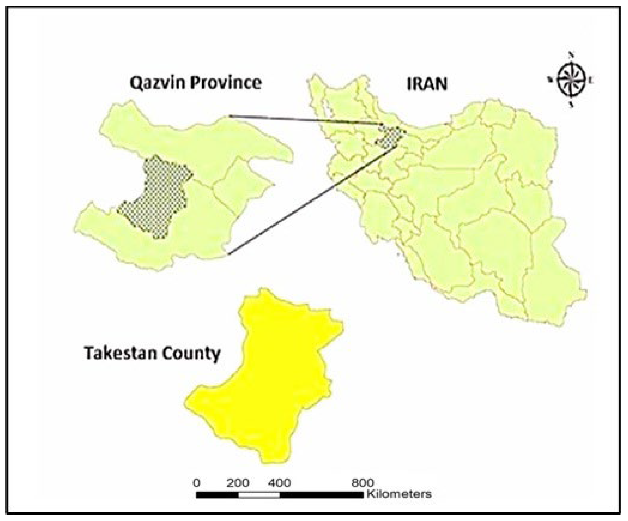
18]. Takestan in Qazvin Province, Iran is the primary grape production center in the region, covering 25,626 hectares (73.22%) of the province’s grape orchards and contributing 27,770 tons (85.5%) of its grape production (Figure 1). Located at 1200 m elevation, in northwestern Iran at latitudes 35°24′ to 36°48′ N and longitudes 48°44′ to 50°51′ E, Takestan benefits from favorable climatic conditions for grape cultivation. Producing premium table and raisin grapes, it supports domestic and export markets, though climate change and water scarcity necessitate sustainable farming solutions. These factors position Takestan as the third-largest grape cultivation area in Iran, following the Fars and Khorasan-Razavi provinces, and the leading region in grape production in the country [13].

2.2. Experimental and Sampling Procedure

We surveyed a sample of 220 grape-growers during the 2020–2021 growing season. Grape farmers were randomly selected from six villages in the study area to ensure a representative sample. The sample size was determined using Equation (1), derived from the Neyman technique [19], as follows:
n = ( N h S h ) N 2 D 2 + N h S h 2
where:
  • n is the sample size;
  • N is the number of holdings in the population;
  • Nh is the population size;
  • S h 2   is the variance of h;
  • D 2 = d 2 / z 2 ;
  • D is the precision of ( x ¯ X ¯ );
  • z is the reliability coefficient (1.96 for a 95% confidence level).
The permissible error in the sample size was 5% for the 95% confidence level, resulting in a sample size of 220 farms.

2.3. Methodology of Budgeting Energy

The input and energy requirements for grape production were collected and determined through questionnaires. The questionnaire included information on the output and input for grape production and economic characteristics. The inputs (human labor, machinery, fertilizers, chemicals, manure, fuel, electricity, irrigation water) and outputs (grape yield) were quantified per hectare. These values were then multiplied by the corresponding energy equivalent coefficients to determine the total energy input and output. Energy equivalents of the inputs and output were converted into energy per unit area (Table 1). The energy equivalent for machinery was calculated using Equation (2) [17,20]:
M E = E G T
where:
  • ME is the machinery energy (MJ h−1);
  • E is the equivalent energy for machinery production (e.g., 62.7 MJ kg−1 for tractor);
  • G is the weight of machine (kg);
  • T is the economic life of machine (h).
By following these methodologies, the study provided a comprehensive analysis of energy use and economic efficiency in grape production systems in Takestan County, Qazvin Province, Iran.
Based on the energy equivalents of the inputs and output (Table 1), the energy ratio (energy use efficiency), energy productivity, specific energy, net energy, and energy intensiveness were calculated as follows [21,28,29]:
Energy   ratio = Output   energy   ( MJ   ha 1 ) Input   energy   ( MJ   ha 1 )
Energy   productivity = Yield   ( kg   ha 1 ) Input   energy   ( MJ   ha 1 )
Specific   energy = Input   energy   ( MJ   ha 1 ) Yield   ( kg   ha 1 )
Net   energy = Output   energy   ( MJ   ha 1 )     Input   energy   ( MJ   ha 1 )
Energy   intensiveness = Input   energy   ( MJ   ha 1 ) Total   production   cos t   ( $   ha 1 )

2.4. Analysis of Energy Using Mathematical Models

We applied different mathematical functions to estimate the relationship between energy inputs and yield. The Cobb–Douglas production function provided more accurate estimates, demonstrating superior statistical significance compared to the linear, linear–logarithmic, logarithmic–linear, and second-degree polynomial functions. This function has been used by a number of authors to examine the relationship between energy inputs and yield [24,29]. The Cobb–Douglas production function is expressed as:
Y = f x exp u  
This function can be reformulated as follows:
l n Y i = a 0 + i = 1 n a j l n ( X i j ) + e i i = 1,2 , , n
where Y i denotes the yield of the ith farm, X i j is the vector of inputs used in the production process, a 0 is a constant term, a j represents coefficients of inputs which are estimated from the model, and e i is the error term.
Assuming that yield is a function of energy inputs, Equation (9) can be expanded to Equation (10) as follows:
l n Y i = α 1 l n X 1 + α 2 l n X 2 + α 3 l n X 3 + α 4 l n X 4 + e i
where X 1 , X 2 , X 3 , and X 4 are chemicals, fertilizer, human labor, and water for irrigation energies, respectively.
In addition to the influence of each energy input on grape yield, the Cobb–Douglas function evaluates the impact of direct, indirect, renewable, and non-renewable forms of energy on grape yield as [21,24,29]:
l n Y i = β 1 l n D E + β 2 l n I D E + e i
l n Y i = Υ 1 l n R E + Υ 2 l n N R E + e i
where Y i is the ith farm yield, β i and Υ i are coefficients of exogenous variables, DE, IDE, RE, and NRE are the direct, indirect, renewable, and non-renewable energy, respectively, used for grape production, and e i is the error term.
In production economics, returns-to-scale (RTS) refer to variations in output following a proportional adjustment in all inputs, wherein all inputs increase by a constant factor. In the Cobb–Douglas production function, it is indicated by the sum of the elasticities derived in the form of regression coefficients. If the sum of the coefficients is greater than unity ( i = 1 n a j > 1 ), it can be concluded that there are increasing returns-to-scale (IRS) which means that an increase in inputs results in an increase in output in greater proportion than the increase in input. If the function is less than unity ( i = 1 n a j < 1), it indicates a decreasing returns-to-scale (DRS) ratio, which means that an increase in output that is less than the increase in input. If the result is unity ( i = 1 n a j = 1), it indicates a constant returns-to-scale ratio; this implies that the change in inputs results in constant output.
We evaluated the sensitivity of grape yield to energy input using marginal physical productivity (MPP), which is derived from the response coefficients of the inputs. MPP measures changes in output relative to changes in input, with other inputs held constant at their average values. A positive MPP indicates that increasing the input leads to higher output, while a negative MPP suggests that increasing the input reduces output [30]. The MPP for inputs was computed using regression coefficients as described by [30,31,32]:
M P P x j = G M ( Y ) G M ( X j ) × a j
where M P P x j is the marginal physical productivity of the jth input, a j is the regression coefficient of the jth input, GM(Y) is the geometric mean of the yield, and GM(Xj) is the geometric mean of the jth energy input.
The last part of this study was an economic analysis that calculated the gross return, net return, benefit-to-cost ratio, and productivity for grape production as [21,24,29]:
Gross   production   value = Yield   ( kg   ha 1 ) × Price   of   commodity   ( $   kg 1 )  
Gross   return = Gross   production   value   ( $   ha 1 )     Variable   production   cos t   ( $   ha 1 )  
Net   return = Gross   production   value   ( $   ha 1 )     Total   production   cos t   ( $   ha 1 )  
Benefit - to - cos t   ratio = Gross   production   value   ( $   ha 1 ) Total   production   cos t   ( $   ha 1 )
Productivity = Yield   ( kg   ha 1 ) Total   production   cos t   ( $   ha 1 )
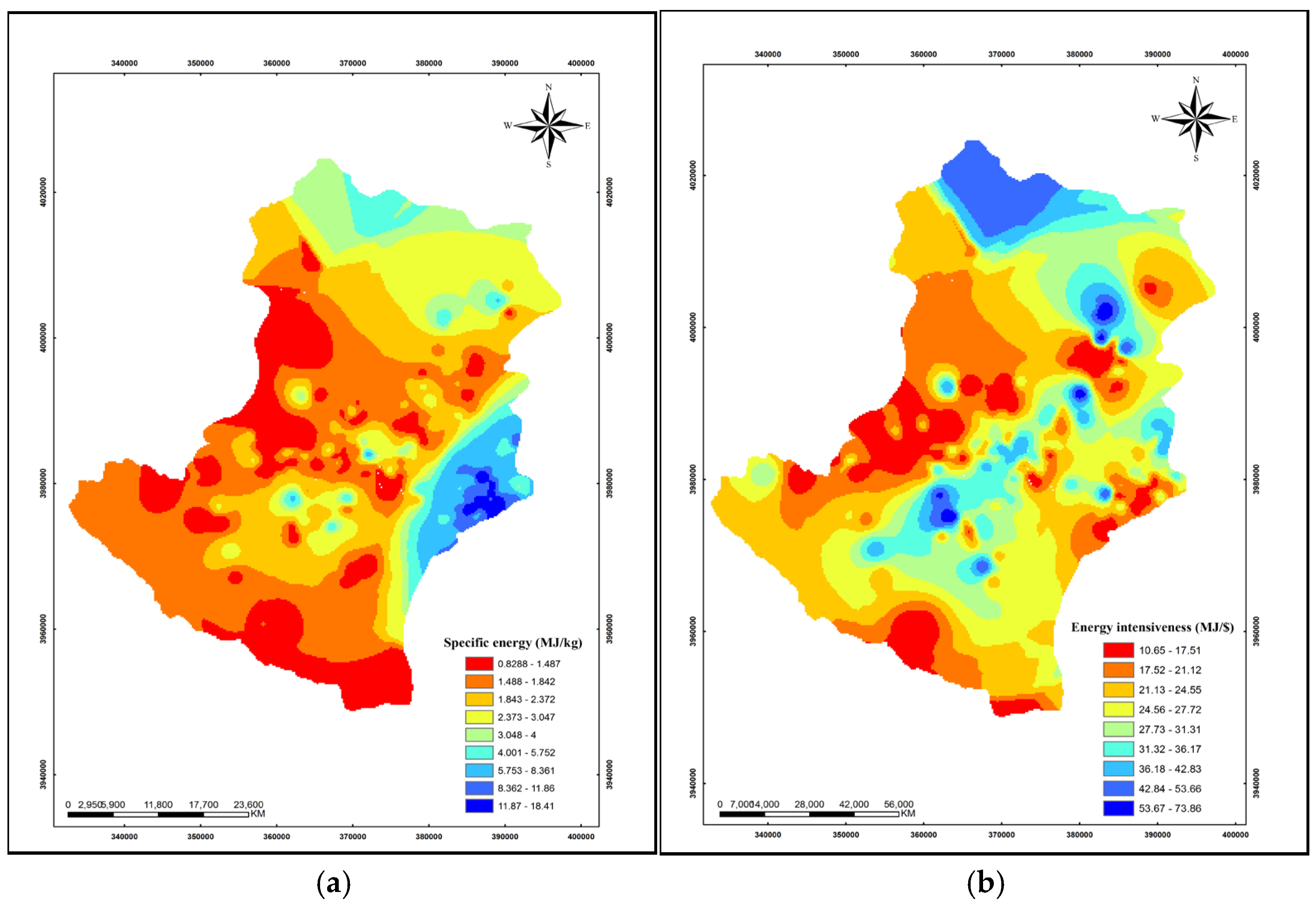
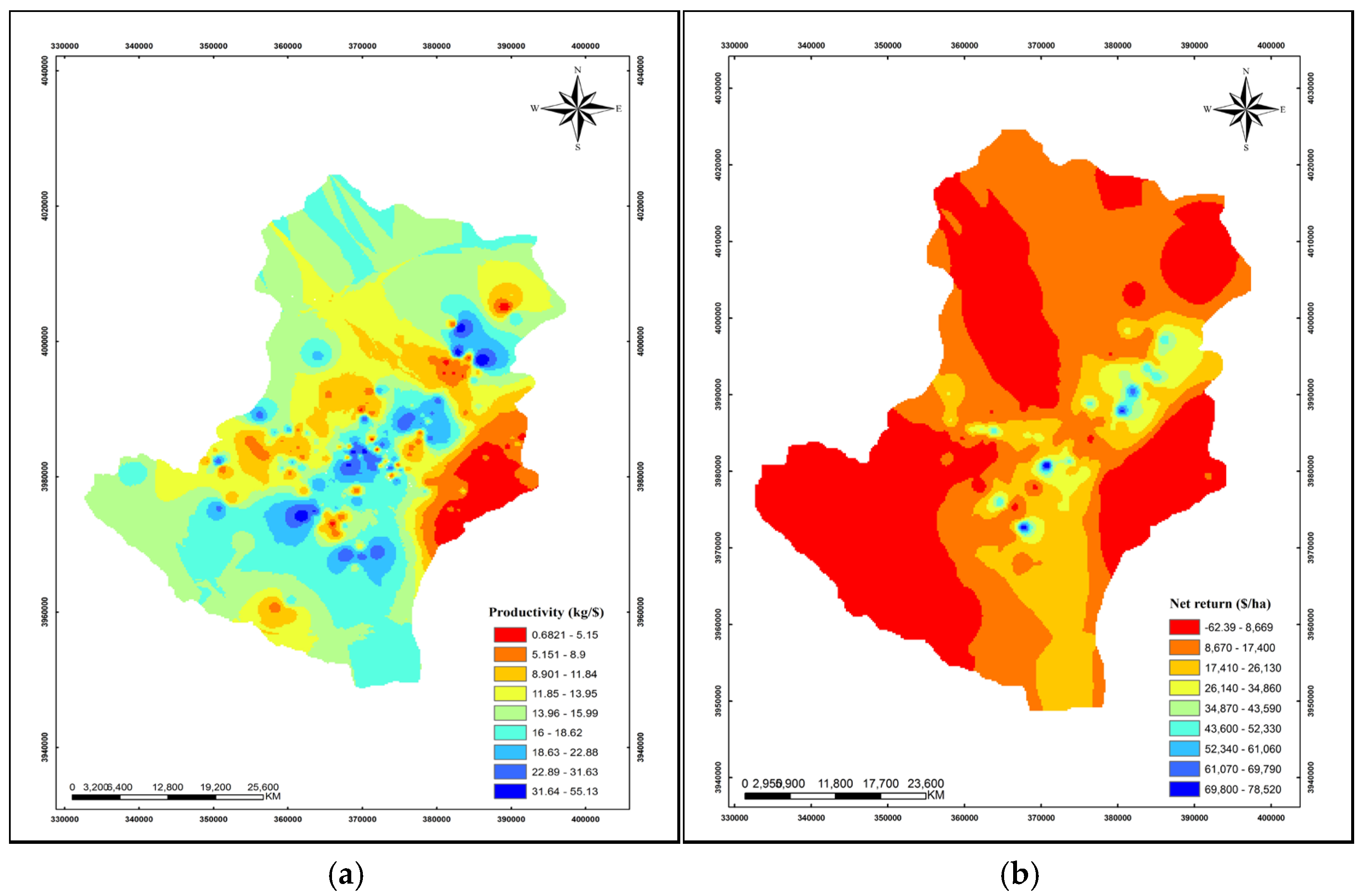
Basic information on energy and cost inputs, energy and economic indices, and grape yield were entered into Excel, Shazam 9.0, and SPSS 20 software programs. Additionally, the Geographic Information System (GIS) was utilized to map the energy flow indices in grape systems for the study area. The energy flow for each location was imputed into ArcGIS 10.3 software and assigned an identification number (ID) in the attribute table. Spatial interpolation using the Inverse Distance Weighted (IDW) method was employed to generate spatial distribution maps of the different energy indices.
IDW is an interpolation technique in which estimates are made based on values at nearby locations weighted by their distance from the interpolation point [33]. The significance of known points can be adjusted by changing the values of two coefficients: (a) the power (exponent) and (b) the radius object. A larger power means that nearby data have a greater influence, resulting in a more detailed interpolated surface. A common value for power, which is a positive real number, is 2. The radius object can be variable or fixed, limiting the number of known points used in the interpolation [34].
The equation used by IDW to estimate a value z(x) at an unknown point is given by:
z ( x ) = i n w i z i i n w i   i = 1,2 , , n
where:
  • z(x) is the estimated value at point xxx;
  • zi is the known value at point iii;
  • di is the distance between point xxx and point iii;
  • p is the power parameter;
  • N is the number of known points.
By using these methodologies and tools, the study effectively analyzed and visualized the spatial distribution of energy use and economic efficiency in grape production systems in Takestan County, Qazvin Province, Iran.

3. Results and Discussion

3.1. Socio-Economic Characteristics of Farmers

A summary of the socio-economic characteristics of grape producers of Takestan county is shown in Table 2. About 49.1% of respondents (Owners) were 35–50 years of age, with the average age being 43.77 years. The average number of years of farming experience was 20.6. The highest frequency (105 people) was farmers who had between 15–30 years of experience. About 97.3% of farmers were male, and only 2.7% of farmers were female. The greatest frequency (103 people) was related to farmers who had no degree (under diploma). About 10% of farmers had a university degree.

3.2. Analysis of Input–Output Energy Used in Grape Production

Table 3 shows the input values for grape production and their energy equivalents and output energy equivalents. The last column in Table 3 gives the percentage of each input to total energy input. The total energy requirement for grape production was 40.6 GJ ha−1. Chemical fertilizers represented the largest portion of this energy input, comprising 36.51%. Farmers used 14.8 GJ ha−1 of chemical fertilizers for grape production. The percentages of chemical fertilizers were nitrogen (73.98%), phosphorus (16.46%), potassium (4.16%), and micro (5.4%). Unfortunately, numerous farmers believe that using chemical fertilizers increases yield, leading them to increase their usage accordingly. The second-highest percentage of energy consumption is for electric energy (20.12%) to run the electric pumps for vineyard irrigation. The use of electricity was 685.21 kWh ha−1. Since total production is performed by humans, machinery had the smallest share of total energy consumption (0.45%). Machinery is not used for traditional cultivation; only small garden sprayers are used in the vineyards. Figure 2 shows the percentage of energy input for grape production by category. The average grape yield was 20 t ha−1, and the total energy output was 236 GJ ha−1.
Energy indices (energy ratio, energy productivity, specific energy, net energy, energy intensiveness) for grape production are presented in Table 4. The energy ratio was 5.81, meaning that 5.81 units of output energy were obtained per unit of energy consumption. Comparable results have been reported for crops, such as 0.15 for greenhouse strawberries [29], 0.64 for greenhouse cucumbers [11], 1.16 for apples [32], 0.66 for garlic [35], 0.87 for tangerines [28], 1.48 for greenhouse tomatoes [11], and 1.76 for alfalfa [27]. The average energy productivity for grapes was 0.49 kg MJ−1. This means that 0.49 units of output was obtained per unit of energy consumption. Calculation of the energy productivity rate is well-documented in the literature, such as tangerines (0.43) [28] and greenhouse cucumbers (0.8) [11]. The specific energy, net energy, and energy intensiveness of grape production was 2.03 MJ kg−1, 195.4 GJ ha−1, and 24.71 MJ USD−1, respectively. The spatial variation and distribution of the specific energy and energy intensiveness indices were derived from ESRI Arc Map 9.3 for the research area and are shown in Figure 3a,b. The specific energy in the western and southeastern portions of the research area was much higher than for the other regions; the lowest value for this indicator is for the eastern portion. Figure 3b shows the highest energy intensiveness for grape production (red portions) are in the western and southern parts and the lowest in the northern part of the study area.
Table 4 shows the distribution of total energy input in direct (DE), indirect (IDE), renewable (RE), and non-renewable (NRE) forms. The shares of DE, IDE, RE, and NRE for grape production are shown in Figure 4. Several researchers have found that the share of IDE is higher than that of DE and that the ratio of NRE is greater than that of RE in agricultural ecosystems [20,21,28,30]. A high ratio of NRE input has a negative effect on sustainability in agricultural production. It is important to better utilize RE sources to increase an energy deficit, because renewable energy production stimulates the agricultural and rural economy, improves the environment, and enhances national energy security [29].

3.3. Econometric Model Estimation of Grape Production

The relationship between energy input and yield was estimated using the Cobb–Douglas production function (Model I) with ordinary least square estimation. The grape yield (endogenous variable) was expressed as a function of exogenous variables including human labor, machinery, fertilizers, manure, chemicals, irrigation water, and electricity in the model. Autocorrelation in the data was assessed using the Durbin–Watson test [21,28], yielding a value of 2.04 for Model I, indicating no first-order autocorrelation at the 5% significance level. The coefficient of determination (R2) for this model was 0.92. The impact of energy input on yield was calculated using Equation (10), and the regression results are presented in Table 5. In grape production, human labor had the highest impact (0.683) and significantly contributed to yield at the 1% level. This implies that a 1% increase in human labor would lead to a 0.683% increase in grape yield. This finding is consistent with previous studies by [21,24,31], which also highlight the significant role of human labor. Water for irrigation followed as the second-most influential input with an elasticity of 0.263, followed by chemicals and fertilizers, with elasticities of 0.176 and 0.155, respectively. The sum of the regression coefficients (RTS) of the energy inputs totaled 1.27 for Model I, suggesting that a 1% increase in total energy input would result in a 1.27% increase in grape yield.
The relationships between DE and IDE and between RE and NRE on yield were investigated using Models II and III, respectively. The results are presented in Table 6. All regression coefficients for IDE, DE, NRE, and RE were positive, with DE, RE, and NRE statistically significant at the 1% level and IDE significant at the 5% level. DE and RE had greater impacts on yield compared to IDE and NRE, with a 1% increase in DE, IDE, RE, and NRE, resulting in yield increases of 0.55, 0.11, 0.56, and 0.24, respectively. Tabatabaie et al. [31] similarly found higher impacts of DE and RE on pear yield in Iran compared to IDE and NRE. Substituting NRE with RE can mitigate negative environmental effects such as global warming and pollution of air, water, and soil [36]. The agricultural sector should consider integrating renewable energy sources like hydropower, geothermal, solar, wind, and biomass to achieve this goal [37]. Enhancing power generation efficiency can also reduce CO2 emissions. Understanding consumer preferences is crucial for setting realistic targets and designing effective programs to increase the use of renewable energy sources [38]. Durbin–Watson values were 1.7 and 1.85 for Models II and III, respectively. The corresponding R2 values for these models were 0.87 and 0.85.

3.4. Economic Analysis of Grape Production

Reducing production costs while increasing yield is crucial in economic viability of the agricultural sector [39]. Lowering input costs, such as labor, energy, and fertilizers, directly enhances profitability, and simultaneously increasing yields maximizes output per unit of resources invested. In this vein, the total cost of grape production and its gross value are detailed in Table 7. Variable and fixed expenditures were calculated separately. Variable costs encompassed human labor, fertilizers, repairs and maintenance of electro pumps and machinery, fuel, electricity, and chemicals. The total expenditure for grape production was USD 1643.7 per hectare, with the gross product valued at USD 15,803.37 per hectare. Variable costs accounted for USD 1543.7 per hectare, comprising 93.91% of the total cost, while fixed costs made up 6.09%. The benefit-to-cost ratio for grape production in the vineyards was 9.61. For comparison, other studies reported benefit-to-cost ratios of 3.11 for pears [40], 1.62 for tangerines [28], 1.94 for kiwifruit [21], 1.36 for garlic [35], 2.75 for prunes [31], and 0.86 for cotton [19]. Productivity was 12.17 kg USD−1. Figure 5a indicates the highest productivity in the eastern part of the research area, while the central part had the lowest productivity, with significant differences between these areas. The gross return of USD 14,259.67-h was obtained by subtracting the variable cost of production from the gross value of production. The net return of USD 14,159.67-h was found by subtracting the total cost of production from the gross value of production. Previous studies have reported net returns of USD 25,175.50 for pears [40]), USD 3223.66 for tangerines [28], USD 5699.97 for kiwifruit [21], USD 1884.97 for rice [19], USD 958.10 for sugar beets [24], and USD 2520.35 for garlic [35]. Figure 5b shows the highest net return indicators in the southwest, eastern, and northern parts of the study area, although the differences in this indicator were not remarkable.

3.5. Sensitivity of Energy Inputs, DE, IDE, RE, and NRE

Sensitivity analysis identifies and measures key variables impacting the environmental system, aiding in their preferential management [32]. It is crucial for enhancing energy use efficiency and minimizing the environmental footprint of energy consumption [26]. The sensitivity of energy input for grape production was analyzed using marginal physical productivity (MPP) based on the response coefficient of the inputs (Table 5). Human labor exhibited the highest MPP (9.17), followed by chemicals (4.53). This indicates that 1 MJ of energy from human labor and chemicals resulted in yield increases of 9.17 kg and 4.53 kg, respectively. These inputs with large sensitivity coefficients significantly impact yield. Similar findings have been reported by [20,22]. The MPP for DE, IDE, RE, and NRE ranged from 0.12 to 0.68 (Table 6), showing that 1 MJ for each of these energy forms increased yield by 0.12 to 0.68 kg. Recommendations for energy input consumption should be made conscientiously, considering environmental and agro-ecological factors specific to each region.

4. Conclusions

Energy management is a prerequisite for the economic viability and success of vegetable growing and processing. Efficient energy use enables farmers to enhance productivity, reduce waste, and lower overall energy demand, directly contributing to cost savings and profitability [41]. This study’s model integrates the energy pyramid framework and econometric analysis to assess energy flow and economic efficiency in grape production, distinguishing it from conventional models. It commences with an energy audit, followed by energy conservation, energy efficiency, and finally renewable energy [42]. This approach aims to optimize resource use, lowers production costs, and offers a baseline for sustainable energy management in agriculture, particularly in resource-constrained regions like Takestan, Iran.
Relatively, the energy pyramid was used to develop an Agricultural Energy Management Plan for grape orchards, including strategies for energy conservation, efficiency, and economic viability. Field operations such as tractor and implement use, pesticide, herbicide, and fertilizer applications, and irrigation water management were assessed to gain energy indices. Based on the results, strategies to address on-farm energy problems and opportunities for energy conservation and efficiency were recommended.
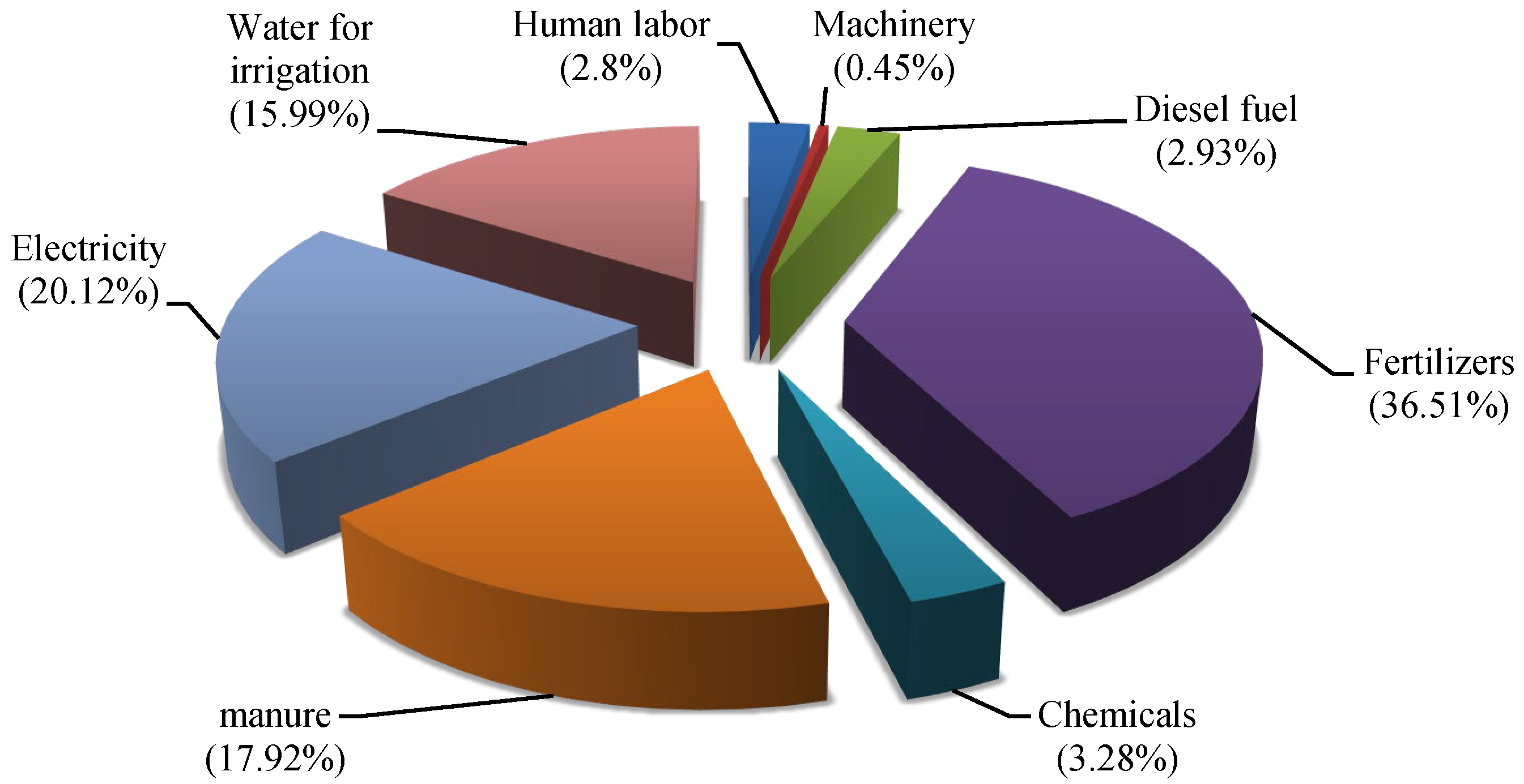
The results revealed that grape production systems consume a total energy of 40.6 GJ ha
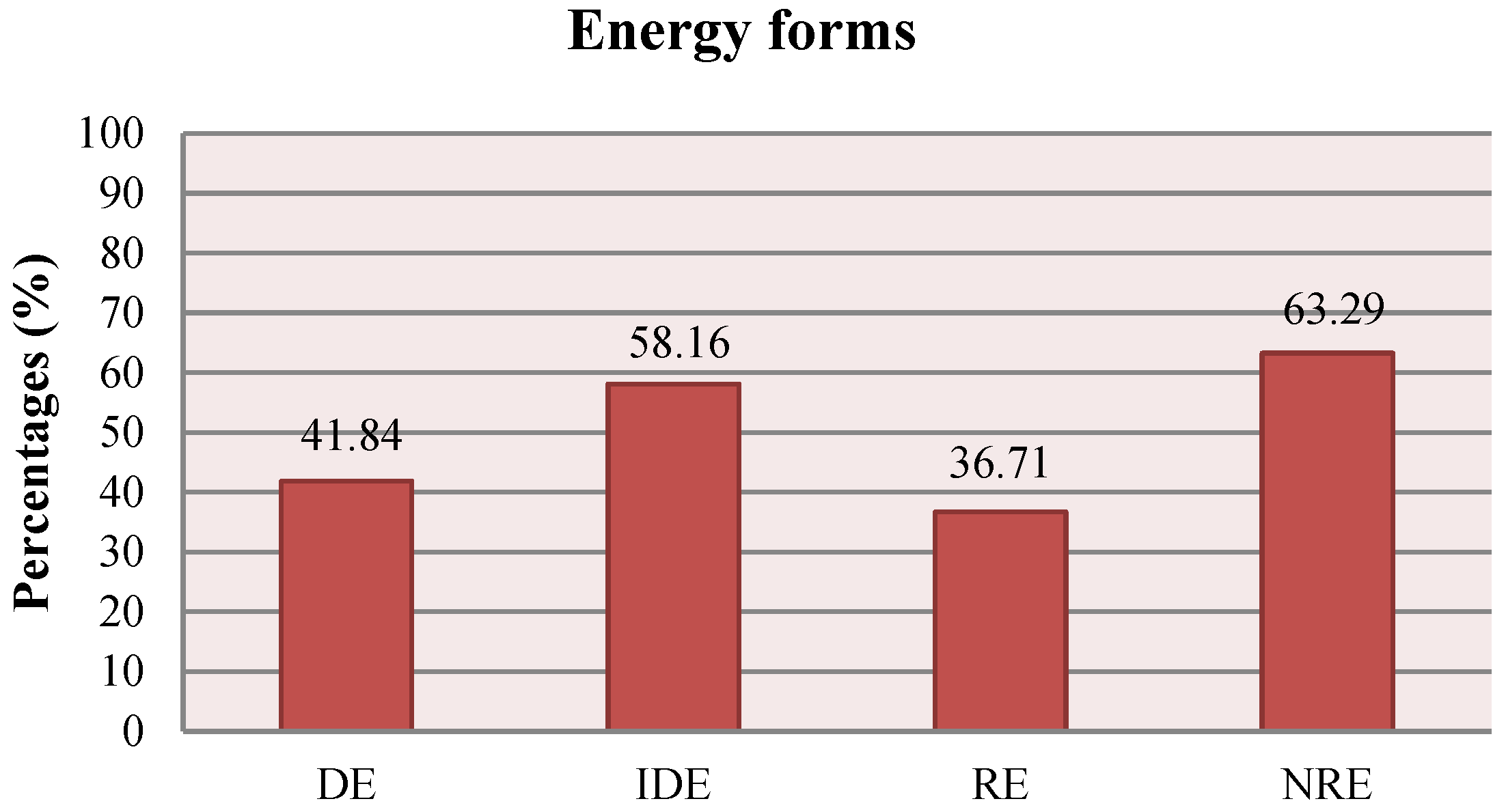
−1. Chemical fertilizers accounted for the highest energy consumption (36.51%), followed by electricity (20.1%). The average total energy input as direct, indirect, renewable, and non-renewable energy forms was calculated as 16.9, 23.6, 14.9, and 25.7 GJ ha−1, respectively. Indirect and non-renewable energy usage was higher than direct and renewable energy usage, indicating a mismatch between inputs, equipment capacity, and user requirements. Optimization of resource use is necessary to achieve a positive energy balance [41]. Optimizing these aspects is crucial not only for achieving a positive energy balance but also for improving the economic viability of grape production systems by reducing production costs and maximizing returns.
The total energy output of the grape production system was USD 236 ha−1. The energy ratio, energy productivity, specific energy, net energy, and energy intensiveness were 5.81, 0.49 kg MJ−1, 2.03 MJ kg−1, 195.4 kg MJ−1, and USD 24.71 MJ kg−1, respectively. Grape production appears efficient in terms of energy consumption on surveyed orchards, with a benefit-to-cost ratio of 9.61, mean net return of USD 14,159.67 ha−1, and productivity level of USD 12.17 kg−1. Grape production systems convert weight to energy more efficiently than other products like strawberries, greenhouse cucumbers, and apples. However, the southern and central parts of Takestan were less profitable, underscoring the labor-intensive nature of conventional grape production practices.
The results indicate that labor force energy was the dominant input in grape production [43]. Other key inputs included water for irrigation (0.26 elasticity), chemicals (0.17 elasticity), and fertilizers (0.15 elasticity). The impacts of DE, IDE, RE, and NRE on yield were 0.55, 0.11, 0.56, and 0.24, respectively, indicating that grape production practices are labor-intensive with conventional approaches.
In conclusion, while grape production systems are economically viable, energy inefficiencies and conventional practices undermine their full potential. Implementing a comprehensive energy management plan—focusing on energy conservation, efficiency improvements, and the integration of renewable energy sources—can significantly enhance both economic viability and sustainability. However, this study had some limitations. Economic and energy factors were integrated due to difficulties in separating them caused by data constraints, and certain costs, such as labor-related care costs, were excluded due to overlap with other costs. Statistical analysis was limited, but a sensitivity analysis was conducted to ensure result reliability. Lastly, the sample size farmers in study area and may not be fully representative of Iranian farmers, and nd future studies could benefit from a broader sample and more detailed statistical analysis of economic and energy factors separately. Given these limitations, recommended strategies include those outlined below.

4.1. Matching Energy Usage to Requirements

Mismatch between equipment capacity and user requirements often leads to inefficiencies. Simple behavioral changes can significantly impact fuel and electricity usage. Measures include:
  • Aligning irrigation schedules with crop water requirements to minimize waste;
  • Matching tractor and implement combinations for optimal output;
  • Using new cultivars from selective breeding programs for standard grape production;
  • Reducing strain on the electric system by using efficient electrical motors for irrigation;
  • With farmers averaging 47 years old and labor being the dominant input in grape production, integrating education, mechanization, and efficient irrigation is essential for sustaining productivity in Iran’s resource-constrained agriculture.

4.2. Maximizing System Efficiency

Efficient operation of equipment through best practices and technology adoption promotes energy efficiency and reduces non-renewable energy footprints [20]. Measures include:
  • Using biological and physical methods to reduce chemical fertilizer energy;
  • Adopting integrated nutrient management to decrease chemical fertilizer energy;
  • Using drip irrigation instead of flood irrigation;
  • Redesigning grape orchards with modern planting systems;
  • Regular maintenance of refrigeration equipment;
  • Using biomass energy sources and reduced tillage practices;
  • Reducing tractor idling time.

Author Contributions

Conceptualization: H.V. and K.K.; methodology: M.G. and A.S.; formal analysis: H.V. and M.G., supervision: H.V. All authors have read and agreed to the published version of the manuscript.

Funding

This research received no external funding.

Institutional Review Board Statement

This article contains no studies with human participants or animals performed by authors. All authors agreed to participate in this study.

Informed Consent Statement

Not applicable.

Data Availability Statement

The data supporting this study’s findings are available from the first author upon reasonable request.

Acknowledgments

The authors sincerely thank Rajabi for her invaluable assistance in conducting the field survey and data analysis. We also extend our heartfelt gratitude to Harem Naghshbandi for his help in drawing the map with GIS.

Conflicts of Interest

The authors declare no conflicts of interest regarding the publication of this paper.

References

  1. Zambon, I.; Cecchini, M.; Mosconi, E.M.; Colantoni, A. Revolutionizing Towards Sustainable Agricultural Systems: The Role of Energy. Energies 2019, 12, 3659. [Google Scholar] [CrossRef]
  2. Pimentel, D.; Pimentel, M.H. Food, Energy, and Society; CRC Press: Boca Raton, FL, USA, 2007. [Google Scholar]
  3. Hercher-Pasteur, J.; Loiseau, E.; Sinfort, C.; Hélias, A. Energetic assessment of the agricultural production system. Agron. Sustain. Dev. 2020, 40, 29. [Google Scholar] [CrossRef]
  4. Schramski, J.R.; Jacobsen, K.L.; Smith, T.W.; Williams, M.A.; Thompson, T.M. Energy as a potential systems-level indicator of sustainability in organic agriculture: Case study model of a diversified, organic vegetable production system. Ecol. Model. 2013, 267, 102–114. [Google Scholar] [CrossRef]
  5. Chen, X.; Shuai, C.; Zhang, Y.; Wu, Y. Decomposition of energy consumption and its decoupling with economic growth in the global agricultural industry. Environ. Impact Assess. Rev. 2020, 81, 106364. [Google Scholar] [CrossRef]
  6. Imran, M.; Ozcatalbas, O. Optimization of energy consumption and its effect on the energy use efficiency and greenhouse gas emissions of wheat production in Turkey. Discov. Sustain. 2021, 2, 28. [Google Scholar] [CrossRef]
  7. Gulkis, A.; Clarke, A. Agricultural energy management plans: Conception to implementation. J. Soil Water Conserv. 2010, 65, 18A–20A. [Google Scholar] [CrossRef]
  8. Geiger, M. Energy and agriculture: A pyramid for action. In Proceedings of the Living and Working on the Land Conference, Sheridan, WY, USA, 3–4 September 2014. [Google Scholar]
  9. Hatirli, S.A.; Ozkan, B.; Fert, C. Energy inputs and crop yield relationship in greenhouse tomato production. Renew. Energy 2006, 31, 427–438. [Google Scholar] [CrossRef]
  10. Tabar, I.B.; Keyhani, A.; Rafiee, S. Energy balance in Iran’s agronomy (1990–2006). Renewable and Sustainable Energy Rev. 2010, 14, 849–855. [Google Scholar] [CrossRef]
  11. Mohammadi, A.; Omid, M. Economical analysis and relation between energy inputs and yield of greenhouse cucumber production in Iran. Appl. Energy 2010, 87, 191–196. [Google Scholar] [CrossRef]
  12. Sattari-Yuzbashkandi, S.; Khalilian, S.; Abolghasem-Mortazavi, S. Energy efficiency for open-field grape production in Iran using Data Envelopment Analysis (DEA) approach. Int. J. Farm. Allied Sci. 2014, 3, 637–646. [Google Scholar]
  13. Soleimani, A.; Abdollahi, H.; Zare, A.G. Horticultural research and development in Iran: A review. Progress. Horticulture 2011, 43, 173–180. [Google Scholar]
  14. Bhatt, B.; Joshi, J.P. Sustainable management of agricultural lands using GIS: A Spatio-Temporal analysis of irrigation water quality in Vadodara taluka. Int. J. Geomat. Geosci. 2012, 2, 901–910. [Google Scholar]
  15. Khan, N.; Fahad, S.; Naushad, M.; Faisal, S. Grape Production Critical Review in the World. Available online: https://ssrn.com/abstract=3595842 (accessed on 8 May 2020).
  16. FAO. FAOSTAT. Available online: www.fao.org (accessed on 22 March 2024).
  17. Mardani, A.; Taghavifar, H. An overview on energy inputs and environmental emissions of grape production in West Azerbayjan of Iran. Renew. Sustain. Energy Rev. 2016, 54, 918–924. [Google Scholar] [CrossRef]
  18. Seccia, A.; Santeramo, F.G.; Nardone, G. Trade competitiveness in table grapes: A global view. Outlook Agric. 2015, 44, 127–134. [Google Scholar] [CrossRef]
  19. Başer, U.; Bozoğlu, M. The impact of farm size on sustainability of beef cattle farms: A case study of the Samsun province, Turkey. Int. J. Agric. Sustain. 2023, 21, 2253647. [Google Scholar] [CrossRef]
  20. Ağızan, K.; Bayramoğlu, Z.; Özbek, O.; Gökdoğan, O. Determination of Energy Use Efficiency, Greenhouse Gas Emissions and Production Costs in Organic Table Grape Production in Turkey. Appl. Fruit Sci. 2024, 66, 269–278. [Google Scholar] [CrossRef]
  21. Mohammadi, A.; Rafiee, S.; Mohtasebi, S.S.; Rafiee, H. Energy inputs–yield relationship and cost analysis of kiwifruit production in Iran. Renew. Energy 2010, 35, 1071–1075. [Google Scholar] [CrossRef]
  22. Royan, M.; Khojastehpour, M.; Emadi, B.; Mobtaker, H.G. Investigation of energy inputs for peach production using sensitivity analysis in Iran. Energy Convers. Manag. 2012, 64, 441–446. [Google Scholar] [CrossRef]
  23. Rafiee, S.; Avval, S.H.; Mohammadi, A. Modeling and sensitivity analysis of energy inputs for apple production in Iran. Energy 2010, 35, 3301–3306. [Google Scholar] [CrossRef]
  24. Asgharipour, M.R.; Mondani, F.; Riahinia, S. Energy use efficiency and economic analysis of sugar beet production system in Iran: A case study in Khorasan Razavi province. Energy 2012, 44, 1078–1084. [Google Scholar] [CrossRef]
  25. Hemmati, A.; Tabatabaeefar, A.; Rajabipour, A. Comparison of energy flow and economic performance between flat land and sloping land olive orchards. Energy 2013, 61, 472–478. [Google Scholar] [CrossRef]
  26. Mousavi-Avval, S.H.; Rafiee, S.; Jafari, A.; Mohammadi, A. Energy flow modeling and sensitivity analysis of inputs for canola production in Iran. J. Clean. Prod. 2011, 19, 1464–1470. [Google Scholar] [CrossRef]
  27. Khodarezaie, E.; Khoshbakht, K.; Veisi, H.; Nazari, M.R. Study of the energy flow and Global Warming Potential (GWP) of alfalfa and maize silage production with different water supply sources (a case study: Qazvin Plain). Environ. Sci. 2023, 21, 1–30. [Google Scholar]
  28. Mohammadshirazi, A.; Akram, A.; Rafiee, S.; Avval, S.H.; Kalhor, E.B. An analysis of energy use and the relation between energy inputs and yield in tangerine production. Renew. Sustain. Energy Rev. 2012, 16, 4515–4521. [Google Scholar] [CrossRef]
  29. Bisheh, A.V.; Veisi, H.; Liaghati, H.; Damghani, A.M.; Kambouzia, J. Embedding gender factor in energy input–output analysis of paddy production systems in Mazandaran Province, Iran. Energy Ecol. Environ. 2017, 3, 214–224. [Google Scholar] [CrossRef]
  30. Pishgar-Komleh, S.H.; Sefeedpari, P.; Rafiee, S. Energy and economic analysis of rice production under different farm levels in Guilan province of Iran. Energy 2011, 36, 5824–5831. [Google Scholar] [CrossRef]
  31. Tabatabaie, S.M.H.; Rafiee, S.; Keyhani, A.; Heidari, M.D. Energy use pattern and sensitivity analysis of energy inputs and input costs for pear production in Iran. Renew. Energy 2013, 51, 7–12. [Google Scholar] [CrossRef]
  32. Jargan, H.; Rohani, A.; Kosari-Moghaddam, A. Application of modeling techniques for energy analysis of fruit production systems. Environ. Dev. Sustain. 2022, 24, 2616–2639. [Google Scholar] [CrossRef]
  33. Naoum, S.; Tsanis, I.K. Ranking spatial interpolation techniques using a GIS-based DSS. Glob. Nest 2004, 6, 1–20. [Google Scholar]
  34. Avanidou, K.; Alexandridis, T.; Kavroudakis, D.; Kizos, T. Development of a multi scale interactive web-GIS system to monitor farming practices: A case study in Lemnos Island, Greece. Smart Agric. Technol. 2023, 5, 100313. [Google Scholar] [CrossRef]
  35. Samavatean, N.; Rafiee, S.; Mobli, H.; Mohammadi, A. An analysis of energy use and relation between energy inputs and yield, costs and income of garlic production in Iran. Renew. Energy 2011, 36, 1808–1813. [Google Scholar] [CrossRef]
  36. Sanaeepur, S.; Sanaeepur, H.; Kargari, A.; Habibi, M.H. Renewable energies: Climate-change mitigation and international climate policy. Int. J. Sustain. Energy 2014, 33, 203–212. [Google Scholar] [CrossRef]
  37. Kapçak, S.; Işleyen, S. The Relationship Between Renewable Energy, Agriculture and Carbon Emissions: The Case of Turkey. Bord. Crossing 2024, 14, 59–72. [Google Scholar] [CrossRef]
  38. Mozumder, P.; Vásquez, W.F.; Marathe, A. Consumers’ preference for renewable energy in the southwest USA. Energy Econ. 2011, 33, 1119–1126. [Google Scholar] [CrossRef]
  39. Rosegrant, M.W.; Wong, B.; Sulser, T.B.; Dubosse, N.; Lybbert, T.J. Benefit–cost analysis of increased funding for agricultural research and development in the global south. J. Benefit-Cost Anal. 2023, 14, 181–205. [Google Scholar] [CrossRef]
  40. Zangeneh, M.; Banaeian, N. Analysis and Evaluation of Energy, Economic, and Environmental Impact Indicators of Horticultural and Greenhouse Production Systems in Iran using PRISMA Method. J. Agric. Mach. 2022, 12, 423–451. [Google Scholar]
  41. Cumming, J. Economic Evaluation of Farm Energy Audits and Benchmarking of Energy Use on Vegetable Farms; Horticulture Innovation Australia Ltd.: Sydney, NSW, Australia, 2015. [Google Scholar]
  42. Snow, S.; Clerc, C.; Horrocks, N. Energy audits and eco-feedback: Exploring the barriers and facilitators of agricultural energy efficiency improvements on Australian farms. Energy Res. Soc. Sci. 2021, 80, 102225. [Google Scholar] [CrossRef]
  43. Song, F.; Xu, X. How Operation Scale Improve the Production Technical Efficiency of Grape Growers? An Empirical Evidence of Novel Panel Methods for China’s Survey Data. Sustainability 2023, 15, 3694. [Google Scholar] [CrossRef]
Figure 1. Takestan county in Qazvin province, Iran.
Sustainability 17 02372 g001
Figure 2. The share of total mean energy inputs in grape production (Source: study’s survey).
Sustainability 17 02372 g002
Figure 3. (a) Spatial distribution of specific energy and (b) energy intensiveness indices for Takestan County.
Sustainability 17 02372 g003
Figure 4. The share of total mean energy inputs as direct (DE), indirect (IDE), renewable (RE), and non-renewable (NRE) forms.
Sustainability 17 02372 g004
Figure 5. (a) Spatial distribution of productivity and (b) net return indices for Takestan county.
Sustainability 17 02372 g005
Table 1. Energy equivalents of inputs and output in grape production.
Inputs (Unit)Energy Equivalent (MJ Unit−1)References
A. Inputs
1. Human labor (h)1.96[17,21]
2. Machinery (h)13.06[17]
3. Fertilizers (kg)
(a) Nitrogen66.14[20,22]
(b) Phosphate12.44[22,23]
(c) Potassium11.15[22,23]
(d) Micro elements120.0[24,25,26]
4. Chemicals (kg)
(a) Herbicides238.0[22,23,24]
(b) Insecticides101.2[22,23,24]
(c) Fungicides216.0[22,23,24]
5. Manure (kg) [20,22,23,24]
(a) Farmyard manure0.3
(b) Poultry manure8.4
6. Diesel fuel (L)56.31[22,23]
7. Electricity (kWh)11.93[22,26,27]
8. Water for irrigation (m3)1.02[22,23,24]
B. Output
Grape (kg)11.8[17]
Table 2. Socio-economic characteristics of farmers.
FeaturesFrequencyMeanPercentageCumulative PercentStandard Deviation
Farmers’ age 43.77 11.16
- 35>5725.925.9
- 35–5010849.175
- 50<5525100
Farmers’ agricultural experience (year) 20.6 11.12
- 15>8538.638.6
- 15–3010547.786.4
- 30<3013.6100
Farmers’ gender - -
- Male21497.397.3
- Female62.7100
Farmers’ educational level (per person) - -
- Illiterate5022.722.7
- Under diploma10346.869.5
- Diploma4520.590
- University degree2210100
Table 3. Values of inputs and output in grape production.
Inputs and Output (Unit)Quantity per Unit Area (ha−1)Total Energy Equivalent (MJ ha−1)Percentage of the Total Energy Input (%)
A. Inputs
1. Human labor (h)581.231139.212.8
(a) Land preparation186.71365.950.9
(b) Spraying14.7528.910.07
(c) Pruning84.59165.80.41.
(d) Irrigation88.34173.150.43
(e) Manure application18.6436.530.09
(f) Fertilizer application7.1614.030.03
(g) Weeding16.2231.790.08
(h) Harvesting164.82323.050.79
2. Machinery (h)14.03183.230.45
(a) Spraying5.3569.870.17
(b) Transporting8.68113.360.28
3. Diesel fuel (L)2.111188.72.93
(a) Spraying6.81383.470.95
(b) Transporting14.3805.231.89
4. Fertilizers (kg)424.214,829.5336.51
(a) Nitrogen165.8810,971.327.01
(b) Phosphate196.142439.986.01
(c) Potassium55.52619.051.52
(d) Micro6.66799.21.97
5. Chemicals (kg)6.661332.673.28
(a) Herbicides4.11978.182.41
(b) Insecticides1.71173.050.42
(c) Fungicides0.84181.440.45
6. Manure7101.97279.0117.92
(a) Farmyard manure6466.291939.894.78
(b) Poultry manure635.615339.1213.14
7. Electricity (kWh)685.218174.5520.12
8. Water for irrigation (m3)6368.816496.1915.99
Total energy input (MJ ha−1) 40,623.09100.00
B. Output
Grape (kg)20,004.27236,050.39
Total energy output (MJ ha−1) 236,050.39
Table 4. Energy input–output ratio and forms in grape production.
ItemsUnitQuantity
Energy ratio-5.81
Specific energyMJ kg−12.03
Energy productivitykg MJ−10.49
Net energyMJ ha−1195,427.3
Energy intensivenessMJ USD−124.71
Direct energy aMJ ha−116,998.65
Indirect energy bMJ ha−123,624.44
Renewable energy cMJ ha−114,914.41
Non-renewable energy dMJ ha−125,708.68
a Includes electricity, human labor, diesel fuel, and water for irrigation. b Includes machinery, fertilizers, chemicals, and manure. c Includes human labor, manure, and water for irrigation. d Includes electricity, machinery, fertilizers, chemicals, and diesel fuel.
Table 5. Econometric estimation and sensitivity analysis results of inputs for grape production based on Model I.
Exogenous Variables α j t-RatioMPP
Chemical0.1762.04 **4.53
Fertilizer0.1552.02 **1.53
Human labor0.6837.72 ***9.17
Water for irrigation0.2633.53 **0.61
Adjust R20.92
Durbin–Watson2.04
RTS = i = 1 n α j 1.27
*** Significance at 1% level. ** Significance at 5% level.
Table 6. Econometric assessment of direct (DE) vs. indirect (IDE) based on Model II, and renewable (RE) vs. non-renewable (NRE) based on Model III.
Exogenous Variables α j t-RatioMPP
DE ( β 1 )0.558.23 ***0.47
IDE ( β 2 )0.111.69 *0.12
Durbin–Watson1.7
Adjusted R 2 0.87
RTS = i = 1 n α j 0.66
RE ( γ 1 )0.5610.83 ***0.68
NRE ( γ 2 )0.244.64 ***0.18
Durbin–Watson1.85
Adjusted R 2 0.85
RTS = i = 1 n α j 0.8
*** Significance at 1% level. * Significance at 10% level.
Table 7. Economic analysis of grape production.
Cost and Return ComponentsUnitQuantity Unit Area (ha−1)
Yieldkg ha−120,004.27
Sale priceUSD kg−10.79
Gross production valueUSD ha−115,803.37
Variable production costUSD ha−11543.7
Fixed production costUSD ha−1100
Total production costUSD ha−11643.7
Gross returnUSD ha−114,259.67
Net returnUSD ha−114,159.67
Benefit-to-cost ratio-9.61
Productivitykg USD−112.17
Disclaimer/Publisher’s Note: The statements, opinions and data contained in all publications are solely those of the individual author(s) and contributor(s) and not of MDPI and/or the editor(s). MDPI and/or the editor(s) disclaim responsibility for any injury to people or property resulting from any ideas, methods, instructions or products referred to in the content.

