Dynamic Response Analysis of Large-Diameter Monopile Foundation Under Ice Load

Abstract

This study investigates the dynamic response of large-diameter monopile foundations subjected to ice loads, emphasizing sustainable design in cold-region offshore wind energy development. Through a combined ice–structure–soil model test and subsequent development of a three-dimensional ice–OWT–soil system model using Abaqus software 2022, this research addresses the sustainability of infrastructure exposed to harsh environmental conditions. The dynamic ice loads are simulated using the coupled CEM–FEM approach, while the Mohr–Coulomb model calculates soil–structure interactions. The calibration and verification processes include comparisons of simulated ice forces, ice-crushing processes, and pile deflections with experimental results. This study comprehensively assesses the effects of ice velocity and thickness on ice actions, as well as the monopile’s top displacement, shear force, and bending moment. The findings indicate that ice thickness significantly influences the dynamic response more than ice velocity, guiding the design toward more sustainable and resilient offshore wind infrastructures. Additionally, a semi-empirical calculation method incorporating the aspect ratio effect is proposed, enhancing the predictive accuracy and sustainability of large-diameter monopile foundations, as validated against field monitoring data from the Norströmsgrund lighthouse. Compared to traditional ice pressure calculation methods, the proposed approach focuses on the influence of the aspect ratio of large-diameter monopile foundations, enabling a more realistic and objective assessment of ice load calculations for OWTs in cold regions. The results demonstrate the efficacy of the proposed approach and offer a new perspective for the design of OWT structures under ice loads.

1. Introduction

Offshore wind energy stands as a cornerstone of sustainable energy solutions, experiencing rapid expansion as one of the most dynamic renewable energy sources [1,2,3]. By the conclusion of 2019, the global installed capacity for offshore wind had surpassed 29 GW [4], highlighting its potential to substantially reduce carbon emissions. The monopile foundation, favored for its cost-effectiveness compared to alternatives such as suction caissons, tripods, and gravity bases, is predominantly employed in the construction of offshore wind infrastructure [5,6,7]. As the installation of offshore wind turbines (OWTs) extends into colder and more challenging environments, including the Danish waters, the Baltic Sea, and the China Bohai Sea, addressing ice loading becomes critical for ensuring the long-term durability and resilience of these structures [8,9,10]. This adaptive strategy not only enhances the environmental sustainability of offshore wind projects but also ensures their viability across diverse geographical contexts, promoting wider adoption of this clean energy technology.

As the utilization of OWTs increases, monopile foundations become predominant, now accounting for over 80%. This trend has intensified research into ice–structure interactions, with a particular focus on dynamic responses and ice loads. Significant aspects of dynamic response include ice-induced vibrations and ice crushing, as emphasized by Gravesen et al. [11,12] and Määttänen et al. [13] Barker et al. [14] investigated these vibrations through OWT model tests, while Bekker et al. [15] conducted numerical simulations to further examine ice–structure interactions. Gürtner et al. [16] developed a cohesive element model to study interactions between ice and the Norströmsgrund lighthouse. Heinonen et al. [17] investigated ice interactions with OWT piles and assessed their sensitivity to ice-induced vibrations. In recent studies, Wang et al. [18] determined the optimal angle for an ice-breaking cone to enhance OWT dynamic response, and Shi et al. [19] analyzed the effects of variables such as ice velocity, thickness, and cone angles on OWT dynamics. Additionally, Zou et al. [20] examined the dynamic response characteristics of the ice–structure–soil interaction for OWTs.

In the field of ice load studies, numerous physical tests have been conducted and theoretical models proposed, as documented by Gravesen and Kärnä [21], Zhou et al. [22], and Taylor and Richard [23]. Murray et al. [24] evaluated ice loads on ice-resistant spars through model tests, while Yue et al. [25] conducted field tests on a cylindrical monopile in Bohai Bay to examine ice loads. Additionally, Xu and Yue [8] investigated ice loads on jacket structures via another field experiment. Popko et al. [26] analyzed variations in ice loads across different offshore structures, determining the most applicable ice load models through various standards. Bekker et al. [27] examined the interaction between ice hummocks and cylindrical structures, and Spencer et al. [28] applied quantile regression to analyze global ice pressure data. Zvyagin and Sazonov [29] developed a mathematical model to explore the stochastic nature of ice loads, while Nord et al. [30] utilized a joint input-state algorithm to investigate ice loads on fixed offshore structures. Shi et al. [31] developed a semi-empirical model and assessed ice loads on OWTs. Most recently, Xing et al. [32] compared ice loads on various offshore structures and investigated potential failure mechanisms of ice sheets and their implications for structural integrity.

The majority of existing research has focused on ice–structure interaction or ice–structure–soil interaction; however, limited studies have addressed the dynamic response and calculation methods for ice pressure on large-diameter monopile foundations. This knowledge gap is particularly critical because large-diameter monopiles, commonly utilized in OWTs, are subjected to complex ice forces that are not yet fully understood. The aspect ratio, specifically the diameter-to-thickness ratio, plays a significant role in the ice pressure calculations for monopiles. Nevertheless, the effects of the aspect ratio on ice pressure calculations have not been thoroughly investigated. Addressing this gap is crucial for enhancing the design of OWTs in ice-prone offshore environments, thereby ensuring their structural integrity and operational efficiency.

To address this research gap, a model test was conducted to examine the dynamic response of a large-diameter monopile foundation subjected to ice loading. Utilizing the experimental data, a validated three-dimensional numerical model was developed to provide insights into the forces, displacements, shear forces, and bending moments induced by various ice loads on the monopile foundation. By synthesizing the results of the model test and numerical simulation, this study proposes a semi-empirical calculation method that incorporates the effect of the aspect ratio of large-diameter monopile on ice pressure, offering a more precise approach for predicting ice load on monopile foundations.

The contributions of this paper are threefold: First, an ice–structure–soil model test was conducted, and a coupled CEM–FEM model incorporating the Mohr–Coulomb model was developed to analyze the structural behavior OWTs under ice load. This approach enables a more comprehensive simulation of ice–structure–soil interactions. Second, a thorough parametric analysis was performed using the coupled CEM–FEM model to evaluate the effects of ice velocity and thickness on the dynamic response of the monopile foundation. Third, a semi-empirical method for calculating ice pressure is proposed, which incorporates the effect of the aspect ratio of large-diameter monopile, an element that has not been adequately addressed in previous research.

The structure of this paper is organized as follows: First, the case study and numerical methods are presented, providing details on the materials and properties of the level ice sheet, the soil model, and the OWT structure. Subsequent sections address the calibration of ice–structure and pile–soil interactions, where ice forces and pile displacements are calibrated using experimental data. Finally, a comparative analysis examines the influence of critical factors such as ice velocities and thicknesses on the dynamic response characteristics and ice loads of monopile foundations.

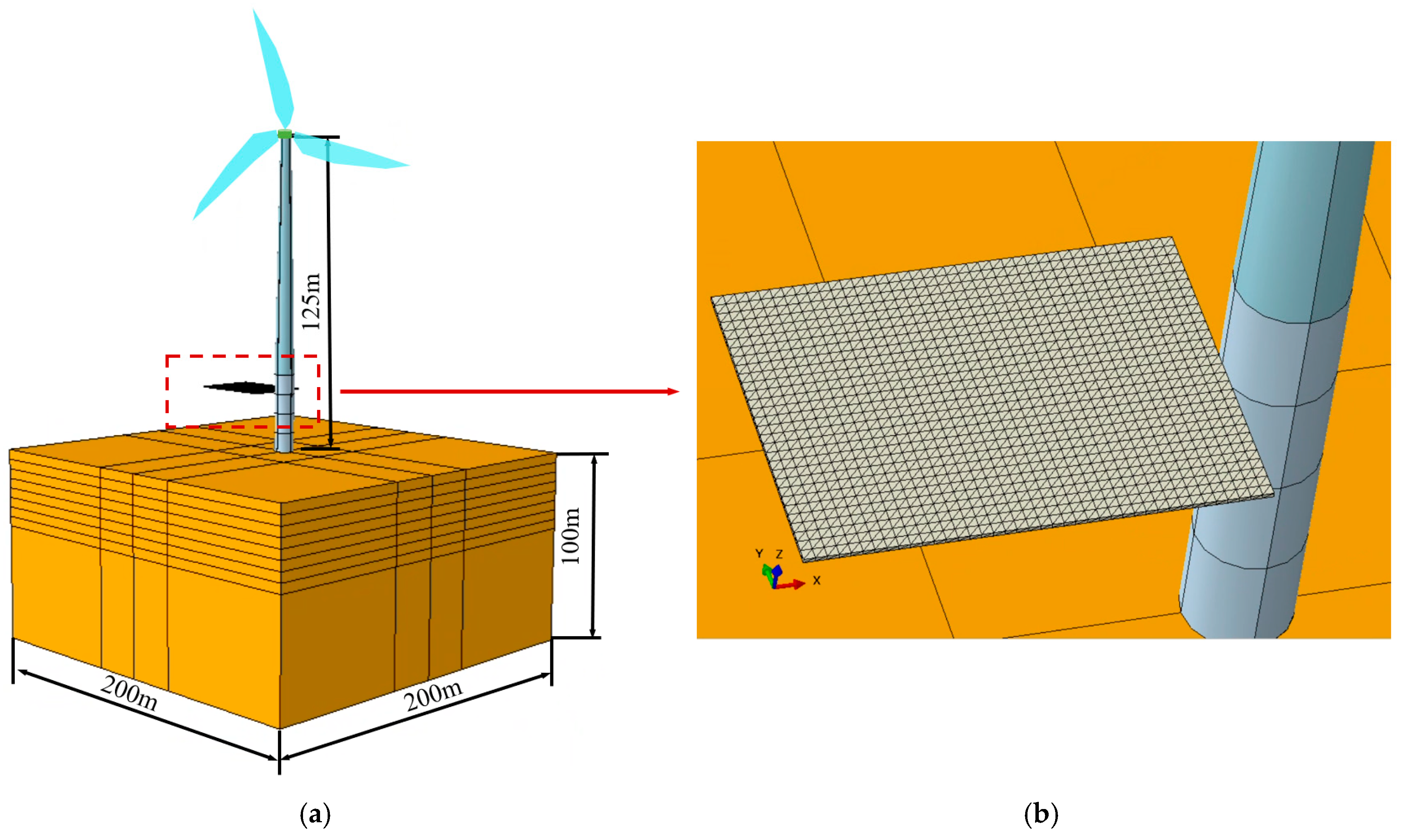
2. Model Description

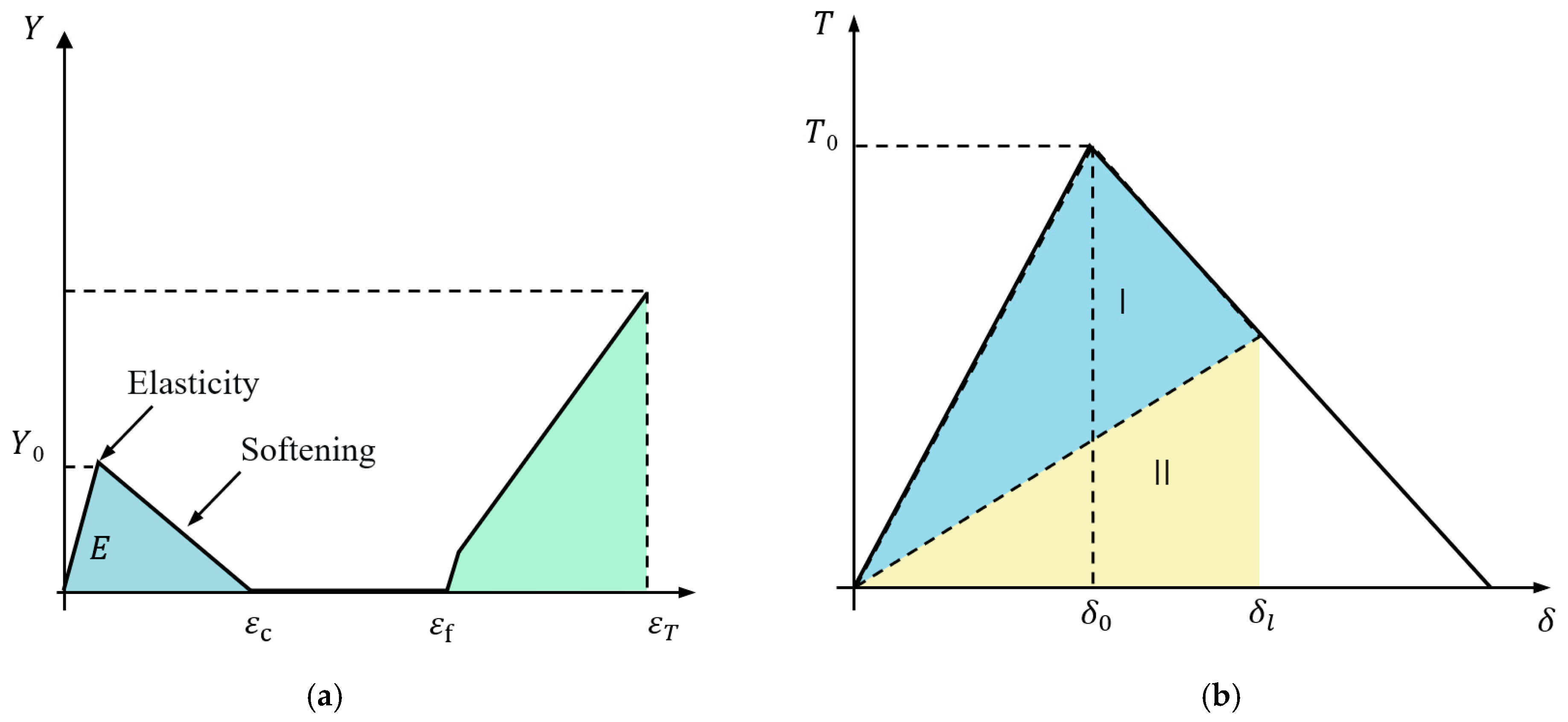
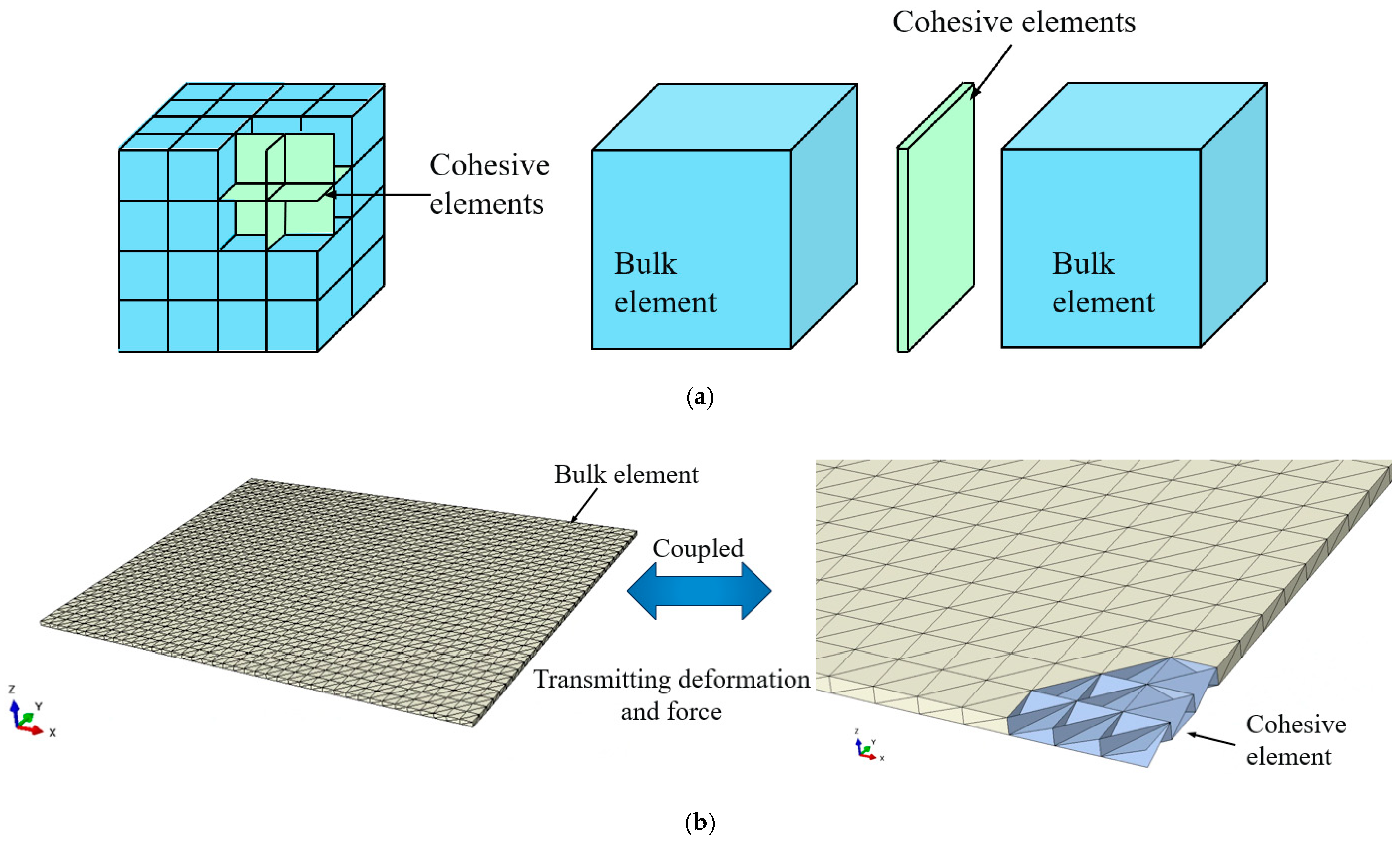
2.1. Modeling of Level Ice Sheet

In this study, a hybrid CEM–FEM model is employed to simulate the complex nonlinear properties of ice. To address the limitations of a standalone finite element model, both bulk and cohesive elements are utilized to capture the intricate nonlinear behavior of ice. The bulk elements model the nonlinear behavior associated with crushing effects, while cohesive elements represent the development of cracks. The ice bulk element is typically assumed to be an elastic–plastic material, with the plastic deformation reflecting microstructure changes in ice, such as recrystallization and pressure melting. During the ice-crushing process, the ice material is assumed to exhibit elastic behavior until reaching the initial yielding point. After the first crack initiates, the ice material follows a linear softening behavior. When the ice is completely crushed, it behaves as a viscous fluid.

Figure 1 illustrates the constitutive laws of both bulk ice and cohesive elements. As shown in Figure 1a, an elastoplastic constitutive law characterizes the nonlinear behavior of bulk ice elements, which undergo three stages. Initially, the ice behaves elastically until the stress reaches a critical yield point Y₀ during compression. Subsequently, the ice transitions to a linearly softened state as stress increases, promoting crack development. This phase continues until the plastic strain reaches ε_c, at which point the ice element fails, transitioning entirely to a viscous fluid state at strain ε_f. Figure 1b depicts the constitutive laws of the CEM, where the characteristics are defined by traction–separation curves. As linear softening progresses and the separation distance increases, the cohesive element is eliminated, resulting in the clear formation of a crack. The overall energy dissipation process involves two distinct regions. Region 2, compared to Region 1, demonstrates a potential for recovery during the crack unloading process, as evidenced by the study conducted by Konuk et al. [33]. To determine the fracture energy of sea ice, Gürtner et al. [34] conducted field tests, yielding several significant conclusions. These results indicate that the fracture energy of sea ice ranges from 23 J/m² to 47 J/m². Further research suggests that higher fracture energy facilitates the simulation of fracture propagation and accumulation in sea ice. Consequently, considering the differences between the numerical models and field test results, a fracture energy of 100 J/m² is adopted for analysis in this study.

Figure 2 depicts a schematic representation of the CEM–FEM model. During ice–structure interaction, nodes are shared concurrently by bulk and cohesive elements, with deformation and forces transmitted synchronously. When a cohesive element reaches its failure threshold, the bulk elements separate, resulting in ice fracture. The CEM–FEM approach is a robust method for modeling ice behavior, particularly in simulating ice fracture and failure processes under various loading conditions. However, like all modeling techniques, the CEM–FEM approach has limitations, including material property assumptions, crack modeling, and computational demands. When extrapolating to different environmental conditions or scales, careful interpretation of simulation results is necessary.

The numerical model in Figure 3b depicts an ice sheet measuring 40 m in length, 30 m in width, and 0.4 m in height, which is utilized in this study. Researchers have conducted numerous studies, including field tests and analyses of ice image data, to determine the optimal ice-breaking length, providing valuable engineering data [35,36]. Based on a comprehensive analysis of field monitoring and relevant numerical simulation results, a mesh size of 0.8 m was selected for this investigation. The ice sheets advance toward the OWT structure at a drift velocity of 0.4 m/s. The edge tangent to the OWT structure forms the free boundary, while the other three edges are constrained in the normal direction, with buoyancy forces acting on the ice sheet. The ice model mesh is generated using tetrahedral elements (C3D4), and cohesive elements (COH3D6) are inserted into the ice. The model comprises 7200 bulk finite elements and 11,860 cohesive elements.

Table 1. Constitutive parameters of the ice model [19,20,32].

Parameters	Bulk Elements	Cohesive Elements
Young’s modulus/(GPa)	5	5
Poisson’s ratio	0.3	0.3
Density (kg/m3)	900	900
Yield strength/(MPa)	2	–
Yield strain	4 × 10−4	–
Fracture energy (N/m)	–	100
Fracture strength/(MPa)	–	1.5/1.1/1.1
Failure strain	0.4	–

details the material properties used within the CEM–FEM framework, adopted from studies by Zou et al. [20], Shi et al. [19], and Xing et al. [32].

2.2. Modeling of Soil

In previous studies, the nonlinear characteristics of pile–soil interactions are often oversimplified and modeled as linear elastic springs or p–y curves, which may not adequately capture the dynamic response of monopile and pile–soil interactions [37,38]. Therefore, the nonlinear characteristics of soil, including plasticity and dilatancy, are modeled using the Mohr–Coulomb model. This model is based on the principles of elastic–perfectly plastic theory and determines soil deformation and failure mechanisms through the shear yield function and tensile yield function. The soil properties are detailed in Table 2, and are mathematically expressed as follows:

τ = c + σtan(φ)

(1)

Here, τ represents the maximum shear stress, while σ denotes the normal stress. The parameter c indicates cohesion, and φ represents the angle of internal friction.

Table 2. Properties of the sand.

Parameters	Value
$\mathrm{Density}, \rho$ (kg/m3)	2000
Poisson’s ratio, μ	0.3
Friction angle, φ (°)	38
Dilatancy angle, ψ (°)	15
Elastic modulus, E (MPa)	130

Table 2. Properties of the sand.

Parameters	Value
$\mathrm{Density}, \rho$ (kg/m3)	2000
Poisson’s ratio, μ	0.3
Friction angle, φ (°)	38
Dilatancy angle, ψ (°)	15
Elastic modulus, E (MPa)	130

Figure 3a presents a comprehensive illustration of the ice–OWT–soil system model. The seabed foundation has dimensions of 200 m in length, 200 m in width, and 100 m in height. The base of the soil domain is constrained in all directions, while the lateral boundaries are constrained only in the normal direction. An eight-node hexahedral element, based on Mohr–Coulomb theory, models the elastic–plastic behavior of the seabed foundation. To enhance calculation accuracy, the mesh size of the soil surrounding the pile was refined, while the mesh size in the remaining areas was gradually increased with distance from the pile. The soil model consists of 75,288 elements. To simulate the nonlinear behavior of pile–soil interaction, the SURFACE_TO_SURFACE algorithm and penalty contact method are utilized to capture both tangential and normal contact behaviors. Furthermore, hydrostatic pressure is applied as external loads on the foundation.

2.3. Modeling of Monopile OWT

The exemplar OWT was developed through a collaboration between the Technical University of Denmark and Vestas [39]. The OWT structure comprises a monopile foundation, tower, nacelle, and rotor with blades. The rotor–nacelle assembly has a mass of 674 t, and

Table 3. Main parameters of the OWT [39].

Parameter	Value
Monopile diameter (m)	10
Monopile thickness (m)	0.125
Rated power (MW)	10
Tower mass (t)	628
Rotor mass (t)	228
Nacelle quality control method (t)	446
Hub diameter (m)	5.6
Hub center height (m)	178.3
Cut in, rated, cut out wind speed (m/s)	4, 11.4, 25

outlines the key design specifications of this turbine. In the numerical model, the rotor–nacelle system is simplified to a concentrated mass at the tower’s apex, with the hub height set at 119 m. The monopile foundation, featuring an outer diameter of 10 m and a wall thickness of 0.125 m, provides a robust base. The tower is constructed from beams with uniform cross-sectional dimensions; its outer diameter measures 8.3 m at the base (with a thickness of 0.075 m), tapering to 5.5 m at the top (with a thickness of 0.03 m). The monopile foundation extends 40 m into the soil and has a total height of 80 m. Both the monopile and tower are discretized into hexahedral grids with a grid size of 1.0 m, comprising 2560 and 2880 elements, respectively. To ensure structural integrity, the monopile–tower connection is modeled using a tie constraint, while the interface between the embedded monopile and soil is modeled with SURFACE_TO_SURFACE contact. Accounting for the effects of paint, bolts, welds, and flanges on the OWT, an effective density of 8500 kg/m³ was implemented.

3. Model Validation

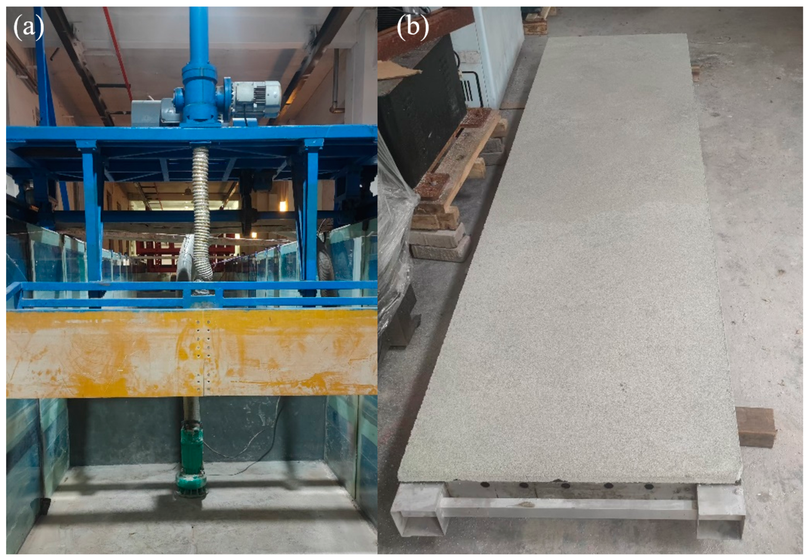
3.1. Test Setup and Experimental Approach

A large-scale model test was conducted to examine the dynamic response of the ice–structure–soil system. The test prototype utilized was the DTU 10 MW wind turbine. The experiment was performed in the State Key Laboratory of Coastal and Offshore Engineering, using an experimental tank measuring 20 m in length, 2 m in width, and 1.8 m in depth. An ice-pushing system was installed in the tank to propel the model ice, composed of the non-freezing synthetic ice material DUT-1, toward the pile at a predetermined speed (Figure 4a). DUT-1, developed by Dalian University of Technology, consists of polypropylene powder, cement, and water [32], and its elastic modulus to tensile strength ratio exceeds 2000, reflecting the fracture and characteristic length of natural ice. The test soil comprised glass microspheres ranging from 0.25 to 0.5 mm in diameter. The model consists of a large-diameter pile, a sand layer, and an ice sheet. The geometric similarity coefficient (λ) is set at 25, with both the gravitational and density similarity coefficients fixed at 1. Additional similarity coefficients were derived based on the Froude and Cauchy similarity criteria, as detailed in

Table 4. Similarity ratios.

Physical Parameters	Similarity Ratio
Displacement (D)	λ
Mass (kg)	λ3
Elasticity modulus (E)	λ
Velocity (m/s)	λ1/2
Time (t)	λ1/2
Gravitational acceleration (g)	1
Force (N)	λ3

. The ice sheet measures 0.016 m in thickness, 3 m in length, and 0.8 m in width (Figure 4b). The monopile model has a diameter of 0.4 m and a height of 1.2 m.

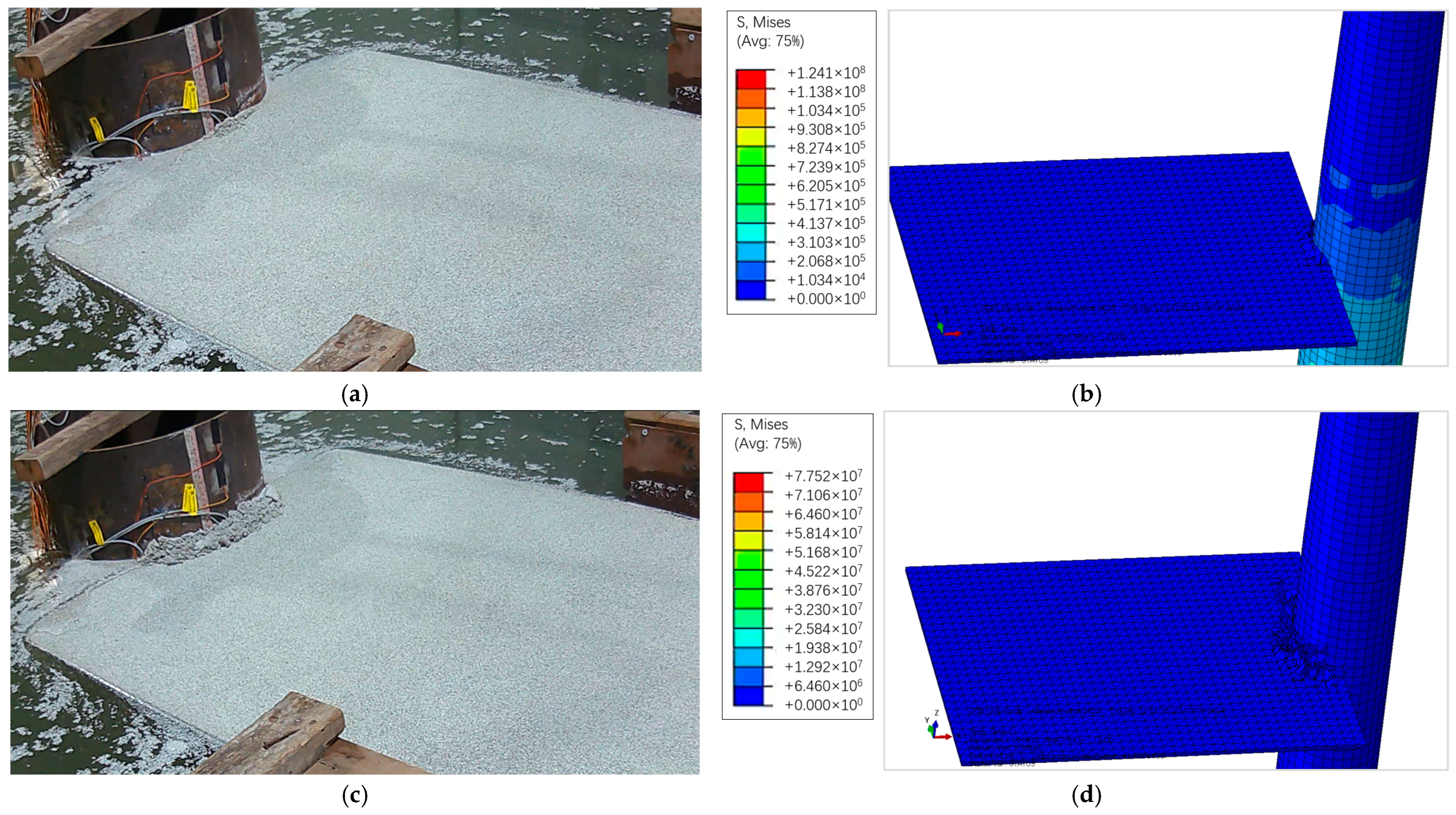
3.2. Validation of Ice Failure and Fragments Accumulation

Figure 5 illustrates a comprehensive simulation of the ice–pile interaction. During this experiment, the OWT exerts a horizontal crushing force on the ice sheet. As collisions continue, crushing failure occurs within the interaction zone between the ice sheet and the monopile. Consequently, the ice sheet bulges upward, causing fragmentation and accumulation in the upper section of the floe. This crushing failure is also replicated in the numerical model. Under the influence of the horizontal crushing force, microcracks develop in the ice sheet, leading to the formation of circular cracks and resulting in crushing failure.

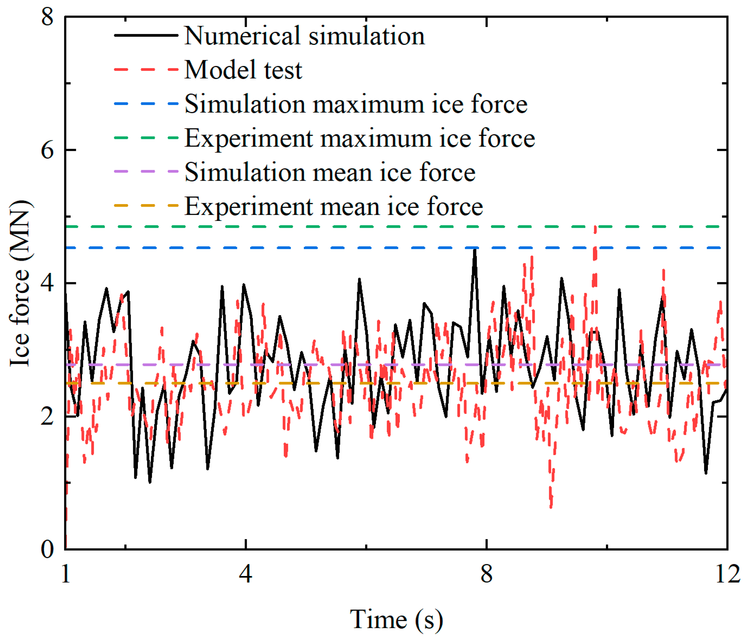
3.3. Validation of the Ice Force

To further validate the ice–structure interaction model, the numerical results are compared with ice force test data. Figure 6 depicts the ice force applied to the 10-MW OWT. The simulated and measured results demonstrate a strong correlation, with maximum ice force values of 4.53 MN for the simulation and 4.85 MN for the test results, respectively. The mean ice force values from the numerical model and experimental results are 2.78 MN and 2.5 MN, respectively. These findings confirm the accuracy of the ice–structure interaction model, which will be utilized in the subsequent case study presented in this research.

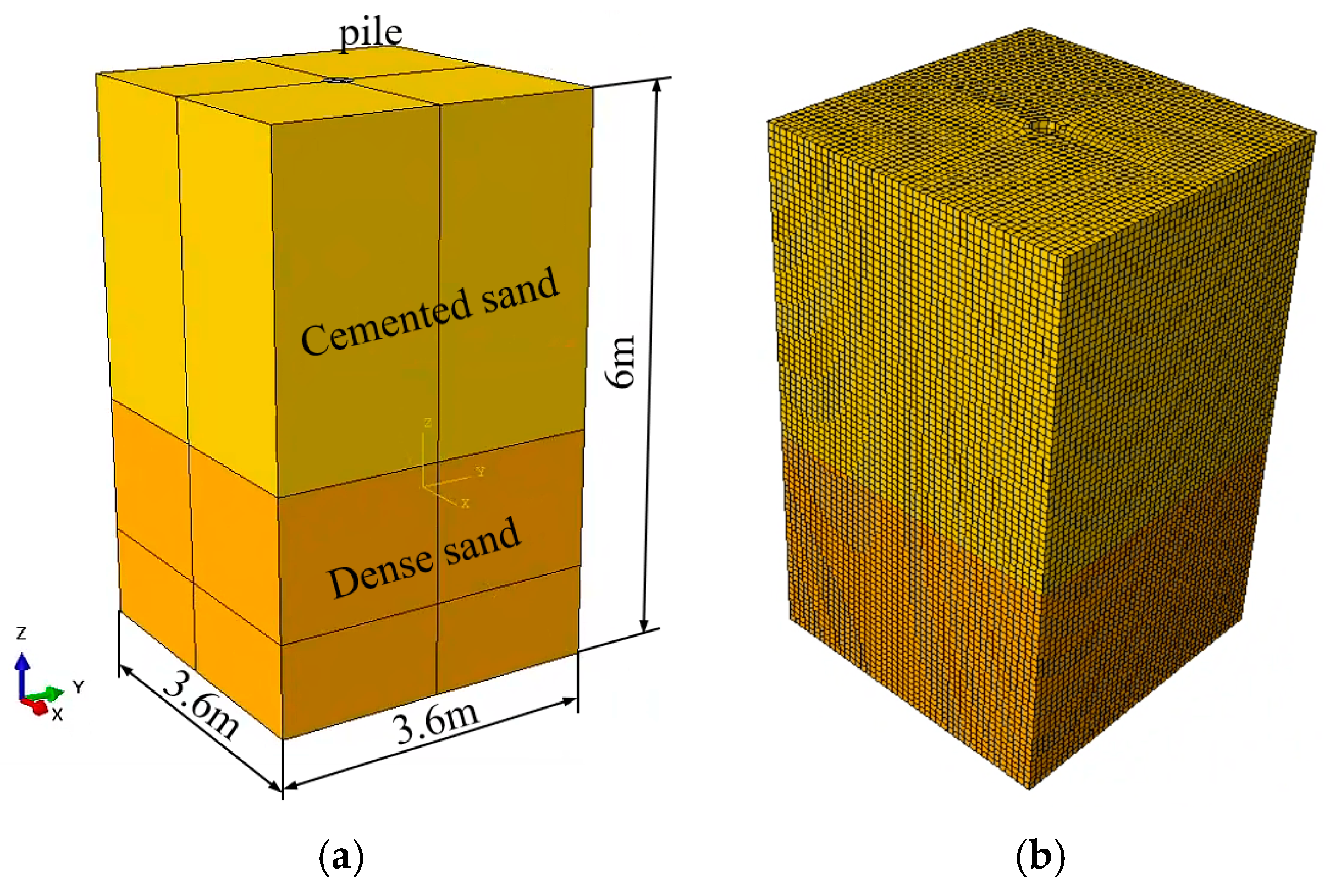
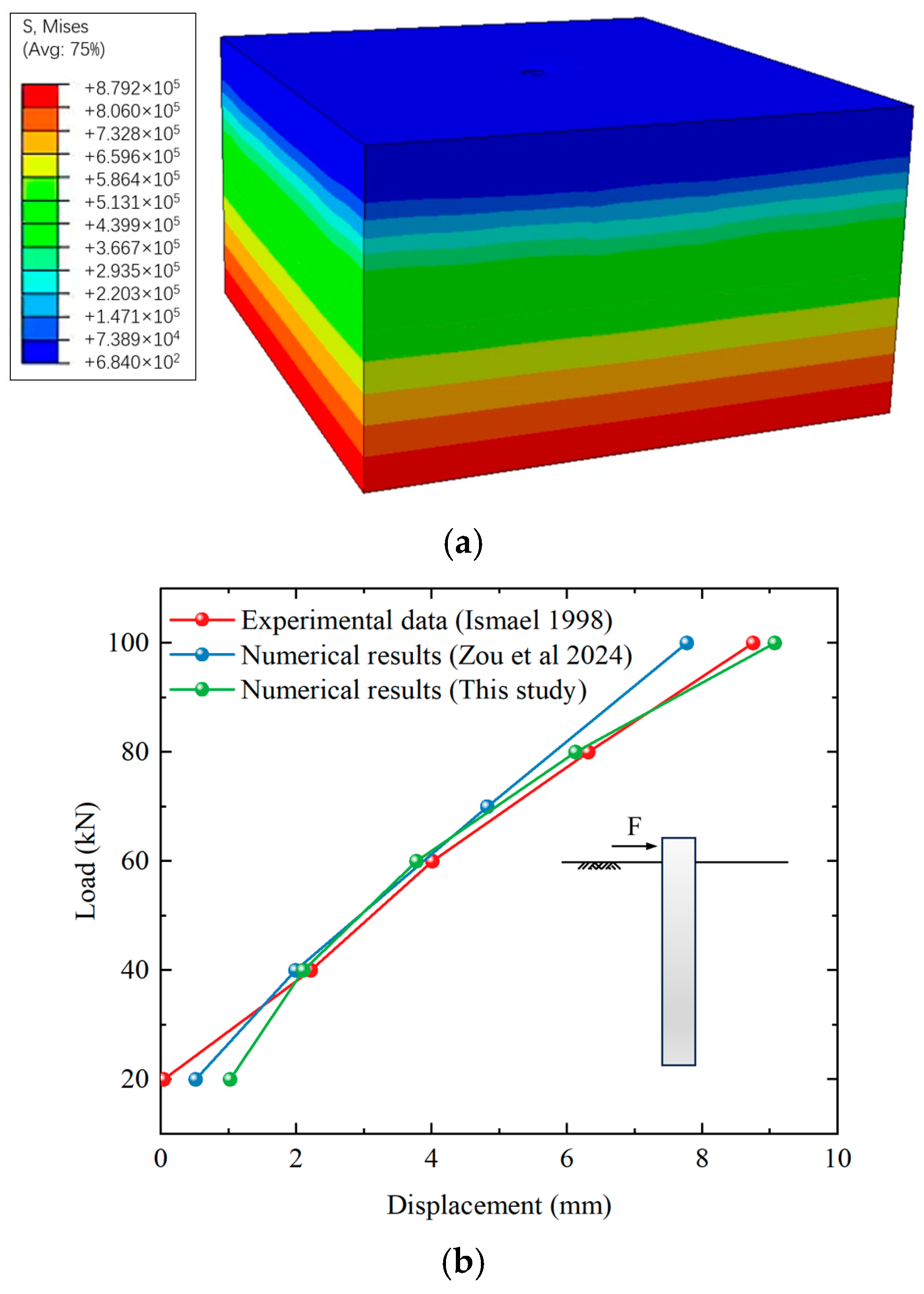
3.4. Validation of the Soil-Pile Interaction

Ismael [40] conducted field tests in Kuwait to evaluate the horizontal bearing capacity of piles. This study specifically examined piles with a diameter of 0.3 m and a length of 5 m. These piles were embedded in a sandy site characterized by two distinct soil layers. The properties of these soil layers are detailed in

Table 5. Material properties of the soil and pile [20].

Material	Weight (kN/m3)	Young’s Modulus (Pa)	Cohesion (kPa)	Friction Angle (°)	Poisson’s Ratio
Medium-dense silty sand	18	1.3 × 107	20	35	0.30
Medium-dense to very dense silty sand	19	1.3 × 107	–	45	0.30
Pile	25	2.3 × 1010	–	–	0.15

.

The soil field, as illustrated in Figure 7, encompasses dimensions of 3.6 m in length, 3.6 m in width, and 6 m in height. Reflecting the actual soil stratification at the site, the soil is divided into two distinct layers: the upper layer measures 3.5 m in height, while the lower layer extends 2.5 m. The base boundaries are fixed, and the edge boundaries are constrained in their respective normal directions. The pile–soil interaction model is analyzed by applying various horizontal concentrated forces and utilizing the explicit solver in ABAQUS/Explicit 2022 (Dassault Systèmes, Providence, RI, USA).

Figure 8a illustrates the von Mises stress distribution in the ice–OWT–soil model. The uniform distribution of von Mises stresses at a specific depth under gravitational influence validates the reliability of the initial stress distribution. Figure 8b compares the lateral displacement between field test results and the numerical model. When the horizontal load reaches 100 kN, the field test measurement shows a displacement of 8.6 mm, while the numerical simulation yields 9.07 mm. Consistent with the findings of Zou et al. [20], the relative error between the field test and numerical results is minimal, at only 5%. This small discrepancy indicates that the numerical model accurately represents the nonlinear soil–structure interaction.

4. Numerical Results and Analysis

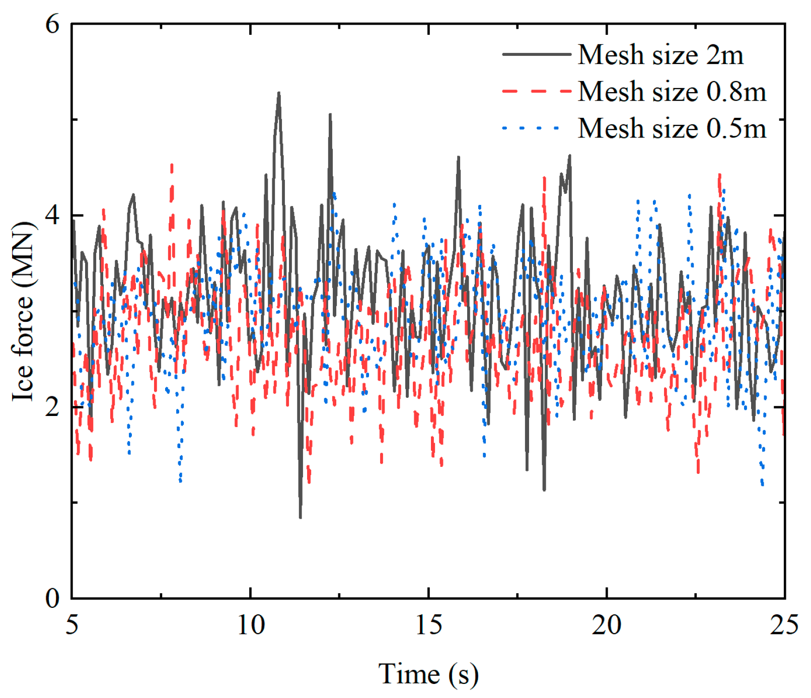
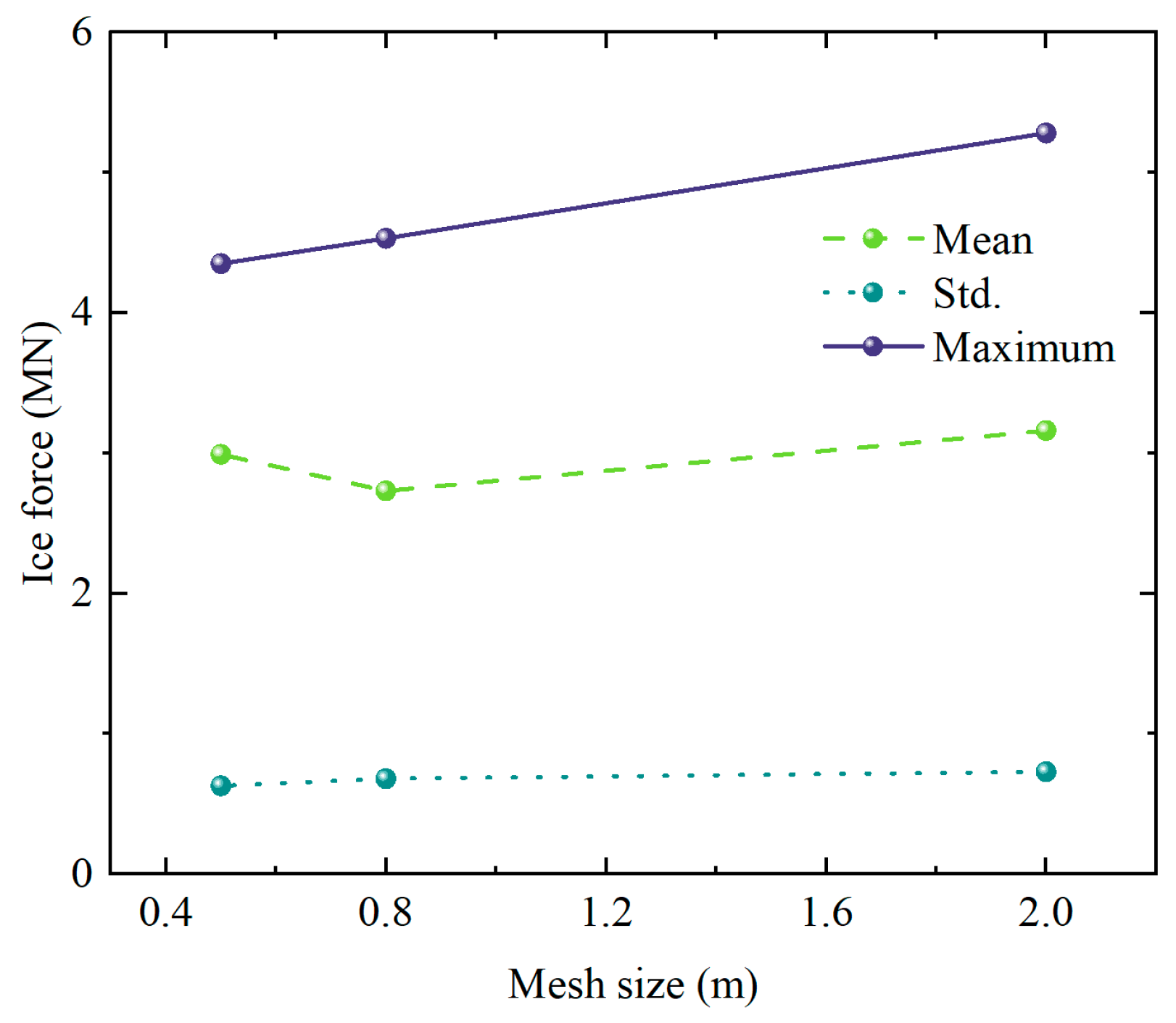
4.1. Influence of Ice Mesh Size

To investigate the influence of mesh size on ice forces, a sensitivity analysis was conducted using three meshes with characteristic element lengths of 0.5 m, 0.8 m, and 2.0 m, corresponding to size ratios (mesh size/ice thickness) of 1.25, 2.0, and 5.0, respectively. Figure 9 illustrates the results of this mesh sensitivity analysis. This analysis reveals that as the mesh size of the ice element increases, the peak value of the ice force also rises. With an ice element mesh size of 2 m, the maximum ice force reaches 5.28 MN, which is significantly higher than the results obtained with smaller mesh sizes. This suggests that larger mesh sizes may introduce errors in the results, potentially affecting computational accuracy. When the ice element mesh sizes are 0.8 m and 0.5 m, the calculated peak values and fluctuation patterns of the ice forces exhibit similar characteristics. Figure 10 depicts the mean, standard deviation, and maximum ice forces for different mesh sizes. The simulation with larger mesh sizes yields higher standard deviation, mean value, and maximum value. While the standard deviation and maximum forces demonstrate an approximately linear relationship with mesh size, the simulation results for mesh sizes of 0.8 m and 0.5 m show minimal differences. Consequently, to balance computational accuracy and efficiency, a mesh size of 0.8 m was selected for all numerical models. This choice ensures result accuracy while effectively reducing computational resource consumption, thereby enhancing overall computational efficiency.

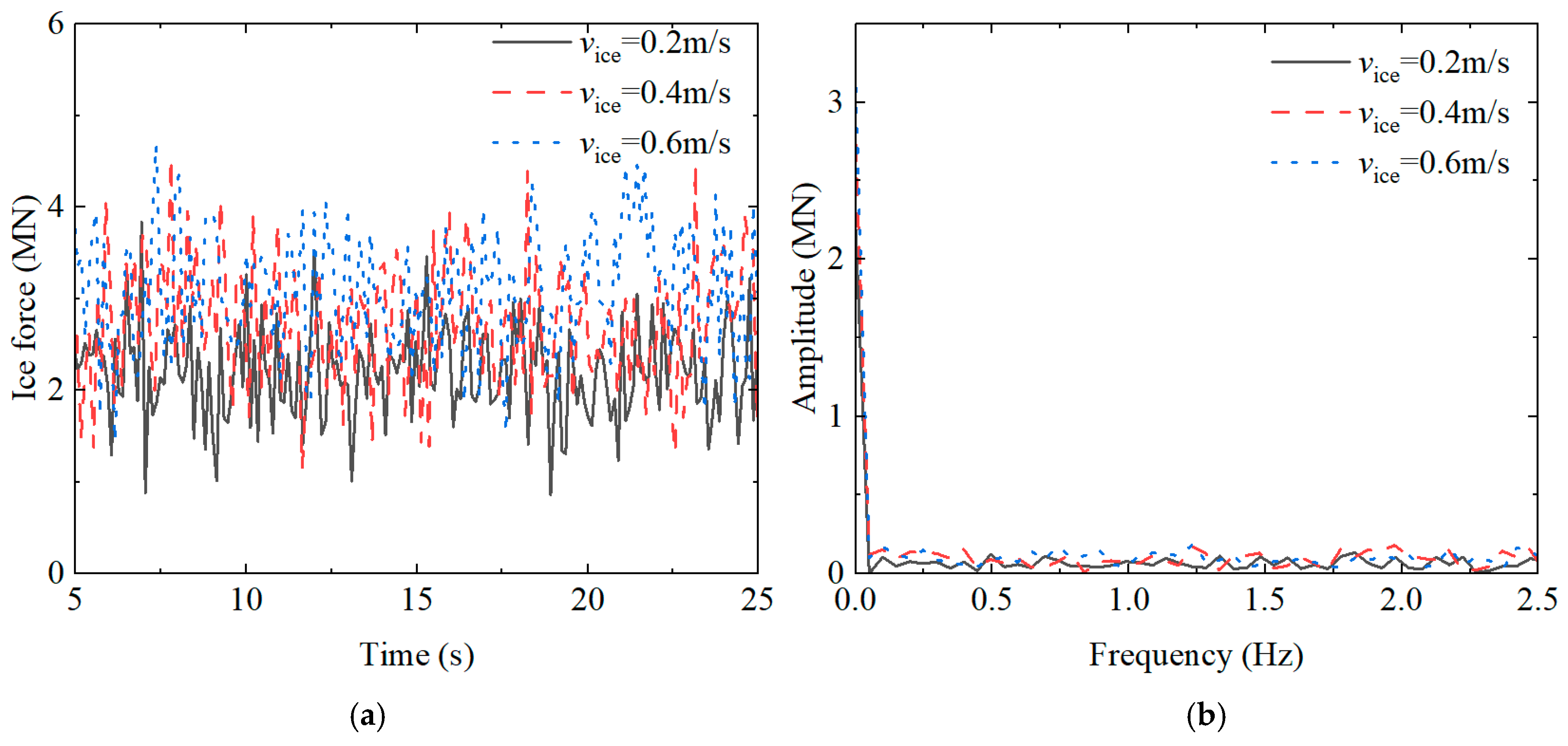
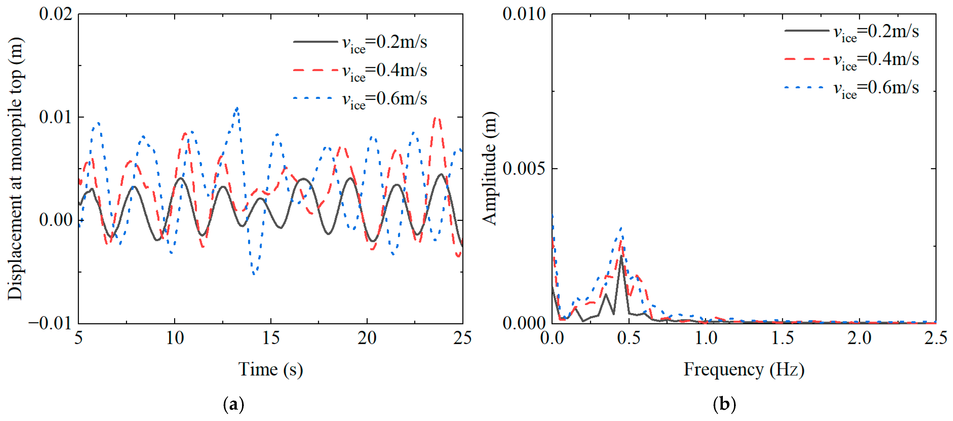
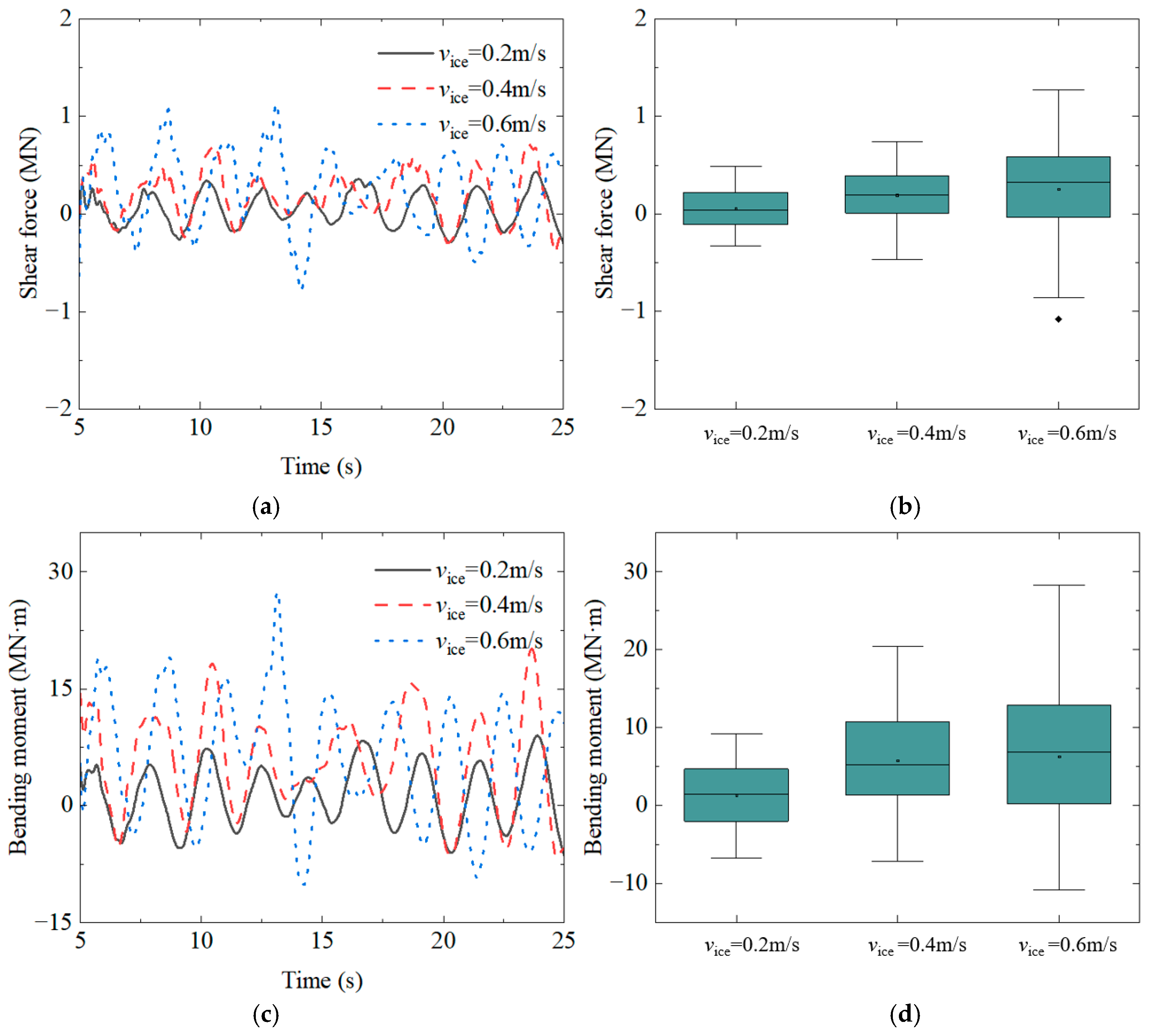
4.2. Influence of Ice Velocities

Figure 11a illustrates the temporal progression of ice forces at varying ice velocities. As the ice velocity escalates from 0.2 m/s to 0.6 m/s, the maximum ice forces recorded are 3.83 MN, 4.53 MN, and 4.69 MN, respectively, while the corresponding average ice forces are 2.19 MN, 2.73 MN, and 3.1 MN. The increase in average ice forces is more substantial compared to the peak ice forces, suggesting that ice velocity exerts a greater influence on average ice forces. The escalating velocity of the ice sheet intensifies the compressive interaction between the ice and the structure, resulting in a significant increase in the average ice force. Figure 11b presents the Fourier spectra of ice forces at different ice velocities. The analysis reveals that as ice velocity increases, the variations in peak frequencies derived from different computational models are minimal. This phenomenon can be attributed to the consistent mechanisms of ice failure across different velocities. Regardless of velocity changes, the ice failure during contact with the structure remains compressive. Despite increased ice sheet velocity, the mode of ice failure does not fundamentally alter, thus explaining the absence of significant shifts in the frequency characteristics observed in the Fourier spectra.

Figure 12a illustrates the temporal progression of monopile top displacement at varying ice velocities. As the ice velocity increases from 0.2 m/s to 0.6 m/s, the corresponding peak displacements of the monopile top are 0.004 m, 0.01 m, and 0.012 m, respectively. This correlation arises because the escalating velocity of the ice sheet amplifies the ice force exerted on the monopile foundation, resulting in a significant increase in both the force applied to and the deformation of the pile foundation. To elucidate the frequency characteristics, Figure 12b presents the Fourier spectra of monopile top displacement at various ice velocities. Through Fourier transformation, the temporal information in the displacement time history curves is converted into frequency data, revealing the frequency characteristics of the monopile foundation’s motion. Under different ice velocity conditions, the primary peak frequencies of the pile top displacement remain relatively constant at 0.45 Hz. However, these peak frequencies surpass the natural bending frequency of OWTs (

Table 6. Natural frequencies of the OWT.

Mode Number	Natural Frequency (Hz)	Mode Shape
1	0.25	Fore–aft bending mode of the tower
2	0.25	Side–side bending mode of the tower
3	1.09	Fore–aft global bending mode
4	1.1	Side–side global bending mode

), indicating a higher vibration frequency of the monopile foundation under ice loading.

Figure 13 illustrates the time history of shear force and bending moment at the mudline of the monopile foundation under varying ice velocities, accompanied by statistical analysis results. As the ice velocity increases from 0.2 m/s to 0.6 m/s, the maximum shear forces observed are 0.48 MN, 0.74 MN, and 1.27 MN, respectively. In comparison to the 0.2 m/s condition, the maximum shear force experiences a 2.65-fold increase. This trend is clearly evident in the box plots, where both the box height and maximum value exhibit significant growth with increasing ice velocity. The bending moment at the monopile foundation demonstrates a similar pattern of increase with ice velocity. Across different ice velocities, the box height and maximum values of the bending moment box plots rise from 6.7 MN·m and 9.21 MN·m to 12.74 MN·m and 28.24 MN·m, respectively, representing increases of 1.9 times and 3.1 times. Notably, the increase in bending moment is more pronounced than that of shear forces at different ice velocities. This phenomenon can be attributed to the simplification of the monopile foundation as a cantilever beam model, where the bending moment is directly proportional to the magnitude of the ice force.

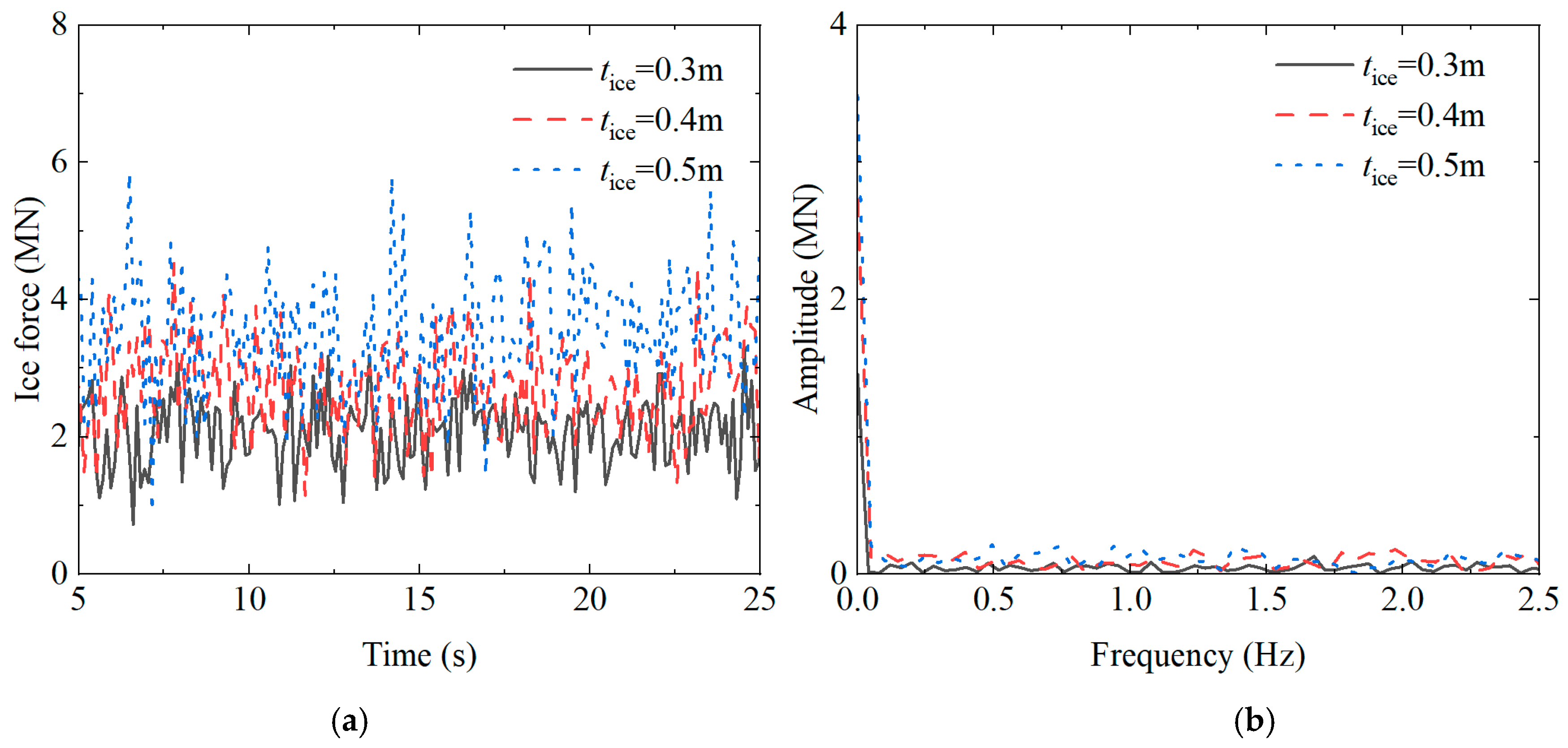
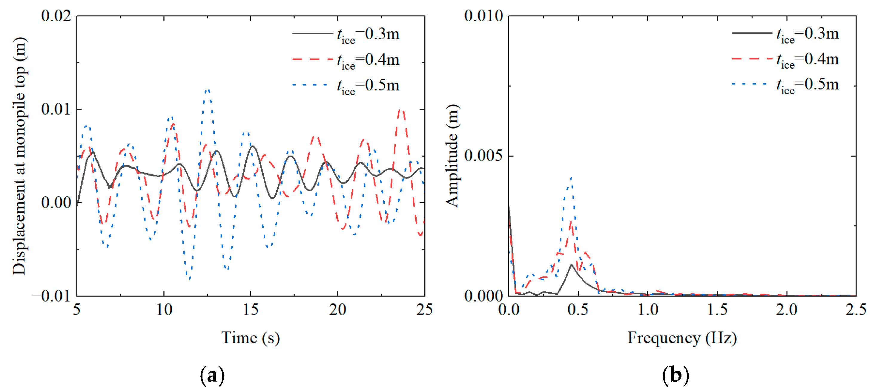
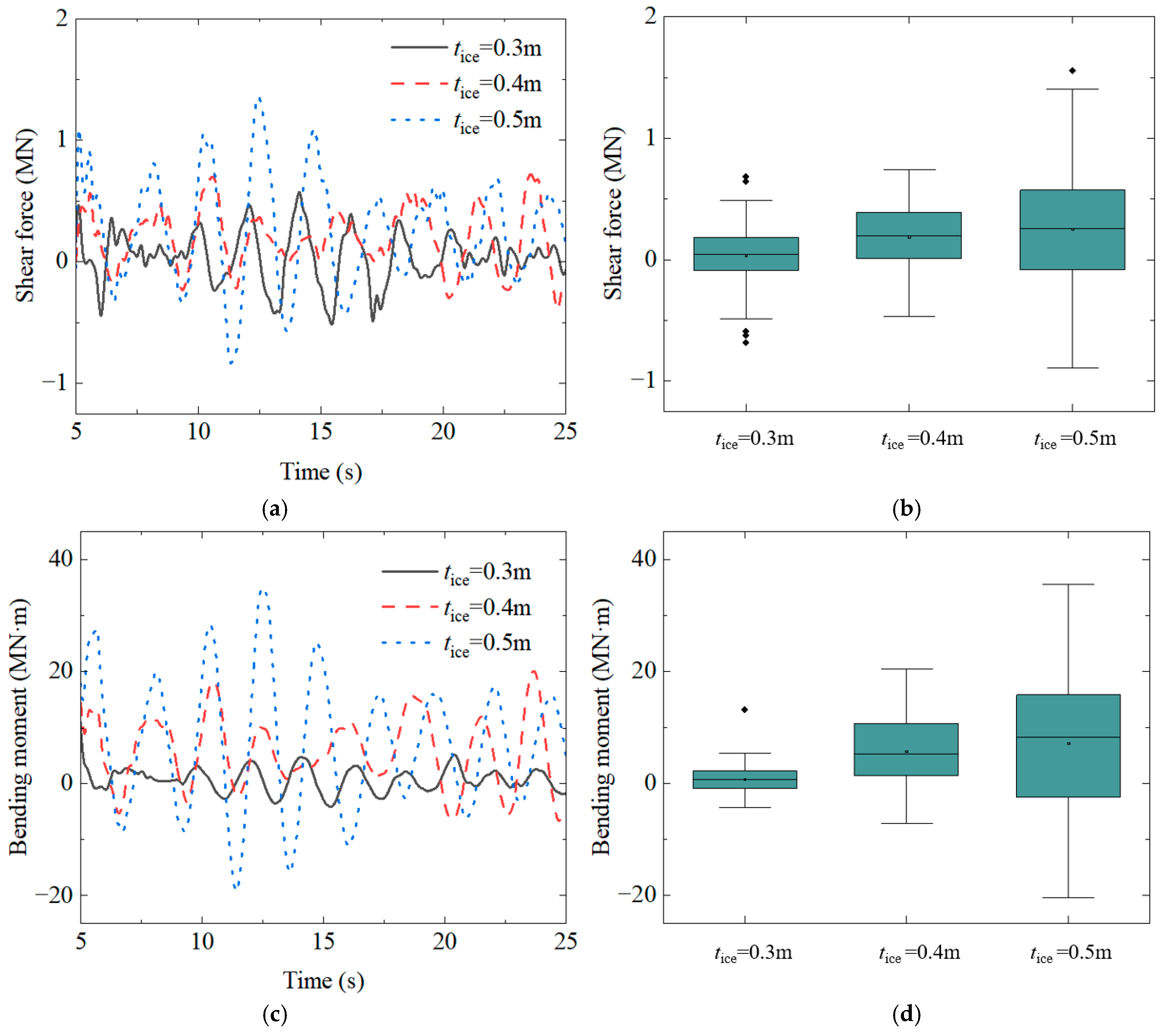
4.3. Influence of Ice Thicknesses

Figure 14a illustrates the temporal evolution of ice forces under varying ice thicknesses. Throughout the ice–structure interaction process, both the mean and maximum values of the ice forces exhibit a positive correlation with ice thickness. For an ice sheet thickness of 0.3 m, the average and peak ice force values are 2.06 MN and 3.31 MN, respectively. As the ice sheet thickness increases to 0.5 m, these values rise to 3.48 MN and 5.86 MN, respectively. Figure 14b depicts the Fourier spectra of ice forces at different ice thicknesses. The peak frequency of the ice forces progressively increases with ice thickness. Notably, when the ice thickness increases from 0.4 m to 0.5 m, the peak frequency of the ice forces rises from 0.39 Hz to 0.49 Hz, demonstrating that ice thickness significantly influences the frequency characteristics of the ice forces. The increase in ice thickness alters the contact force and interaction between the ice sheet and the monopile foundation, resulting in not only greater ice force magnitudes but also modifications to their frequency response.

Figure 15a illustrates the temporal evolution of monopile top displacement under varying ice thicknesses. For an ice thickness of 0.5 m, the maximum displacement reaches 0.015 m. In contrast, when the ice velocity is 0.6 m/s, the maximum displacement is 0.012 m, slightly less than the displacement observed with an ice thickness of 0.5 m. This observation suggests that ice thickness exerts a more significant influence on monopile top displacement compared to ice velocity. This phenomenon can be attributed to the direct correlation between ice thickness and ice forces, which subsequently affects the dynamic response of the monopile foundation. Figure 15b depicts the Fourier spectra of monopile top displacement under different ice thicknesses. The peak frequencies of monopile top displacement exhibit a similar trend across various ice thicknesses, mirroring the pattern observed with changing ice velocities. As the ice thickness increases from 0.3 m to 0.5 m, the peak frequency of monopile top displacement remains relatively constant, demonstrating strong spectral consistency. This consistency indicates that the spectral characteristics of monopile top displacement remain similar under different conditions, regardless of changes in ice velocity or thickness. Although ice thickness and velocity differently impact ice force, both have a minimal effect on the frequency characteristics of monopile top displacement. However, an increase in ice thickness elicits a more pronounced dynamic response in the monopile foundation compared to changes in ice speed.

Figure 16 illustrates the time history of shear force and bending moment at the mudline of the monopile foundation under varying ice thicknesses, accompanied by statistical analysis results. As ice thickness increases, both the shear force and bending moment at the mudline of the monopile foundation increase substantially. At an ice thickness of 0.3 m, the maximum shear force is 0.68 MN, while at 0.5 m thickness, this value rises to 1.56 MN. The bending moment at the mudline exhibits a similar trend. With increasing ice thickness, the maximum bending moment rises from 13.21 MN·m to 35.64 MN·m. In comparison to Figure 13, where the maximum bending moment is 28.24 MN·m for an ice velocity of 0.6 m/s, there is a 20% decrease relative to the maximum bending moment for an ice thickness of 0.5 m. This analysis indicates that ice thickness has a more significant impact on the shear force and bending moment of the monopile foundation than ice velocity.

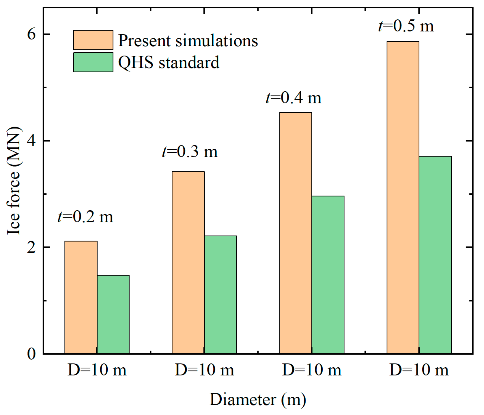
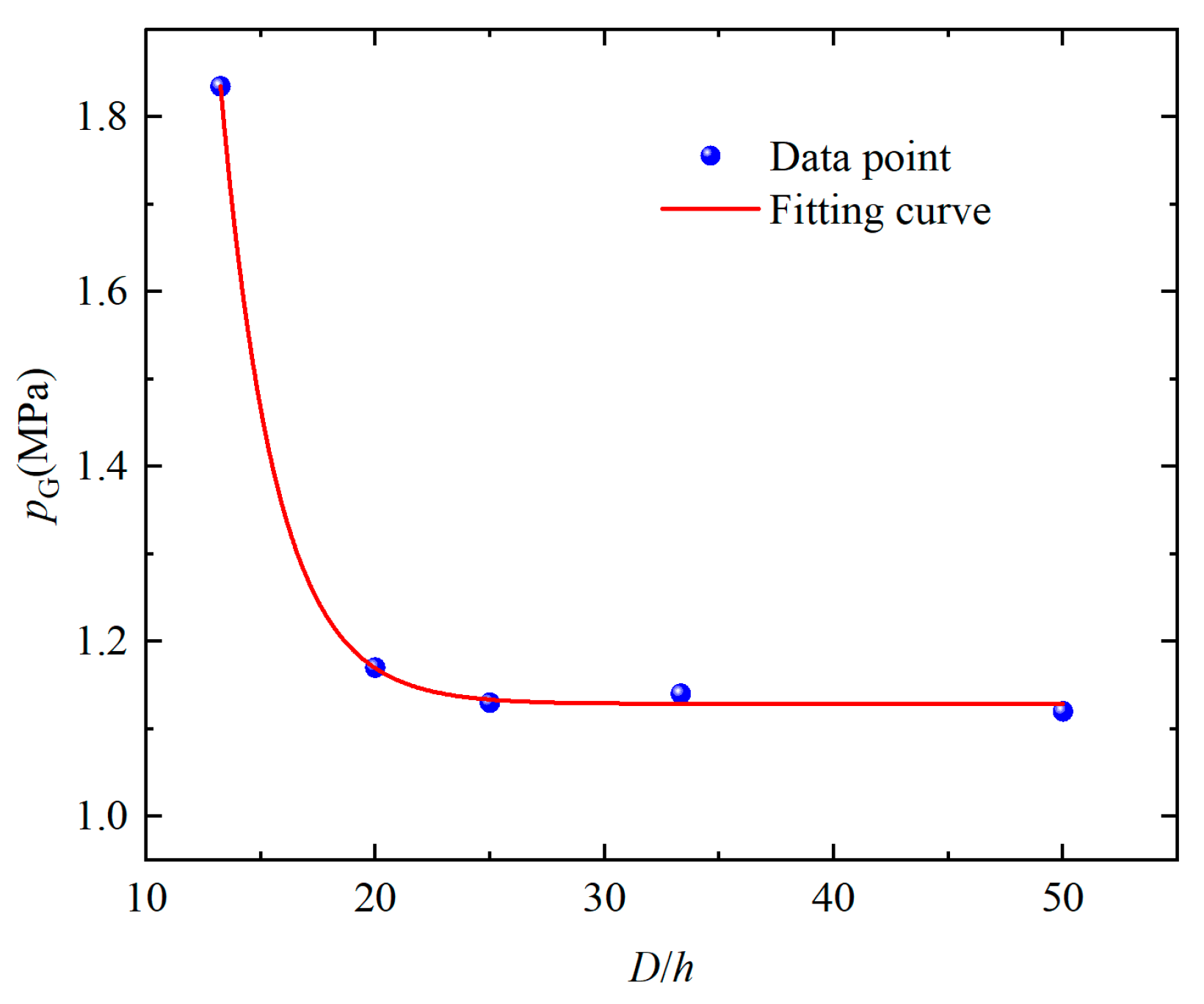
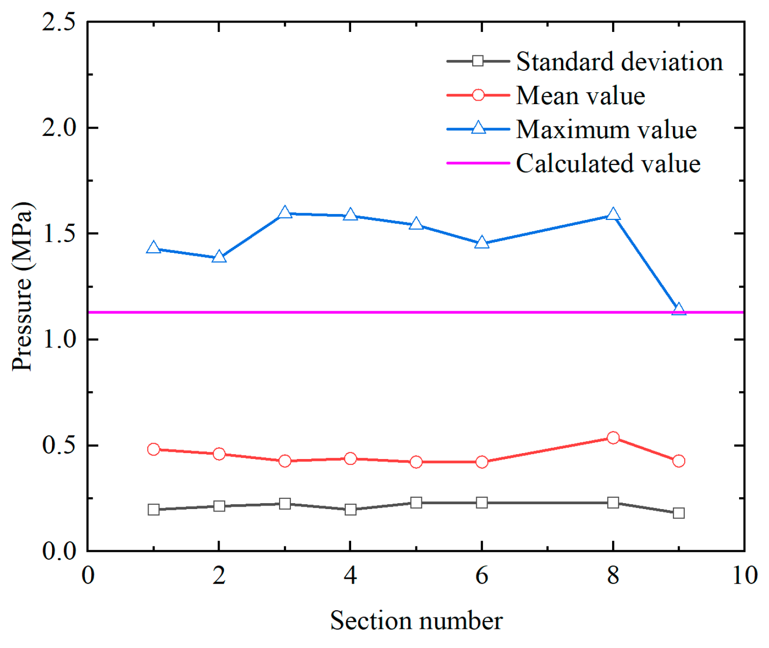
5. Semi-Empirical Method for Calculating Ice Pressure Incorporating Diameter-to-Thickness Ratio Effects

In the context of offshore structures situated in cold regions, precise prediction of ice loads is crucial for ensuring the stability of offshore engineering projects. Numerous international standards and guidelines, including ISO 19906 [41] and QHS 3000-2002 [42], provide empirical formulas for estimating ice loads on offshore structures. These formulas are predominantly derived from model tests and field monitoring data. According to QHS 3000-2002, the ultimate compressive ice force F acting on vertical piles can be calculated using the following formula:

$$F=m·I·f_{\mathrm{c}}·{\mathrm{\sigma }}_{\mathrm{c}}·D·h$$

(2)

where m is the shape coefficient, and the circular section is 0.9; ${\mathrm{\sigma }}_{\mathrm{c}}$ is the unconfined compressive strength of sea ice, which is 2.06 MPa; D is the diameter of the pile; h is ice thickness; I is the embedding coefficient; f_c is the contact coefficient.

Nevertheless, the QHS 3000-2002 standard is theoretically limited to calculating compressive ice loads on vertical pile structures with diameters not exceeding 2.5 m. Large-diameter monopile foundations, due to their increased aspect ratio, present a more extensive contact area between ice and structure. Consequently, their dynamic response under ice loading differs significantly from that of smaller-diameter pile foundations. Thus, it remains uncertain whether existing standards adequately account for the aspect ratio effect on large-diameter monopile foundations, necessitating further verification.

Figure 17 illustrates a comparative analysis of extreme ice forces between numerical results and values calculated according to established standards. The analysis reveals that for large-diameter monopile foundations subjected to varying ice sheet thicknesses, the ice force values derived from simulations consistently exceed those calculated using QHS standards. For instance, with an ice thickness of 0.4 m, the numerical result yields 4.53 MN, while the calculated result is 2.96 MN. Notably, as ice thickness increases, the discrepancy between numerical ice force values and standard calculated values tends to widen. Consequently, drawing upon the calculation methodology for ice loads outlined in the international standard ISO 19906, this study proposes the following modifications to the ice force calculation formula:

$$F=P_{\mathrm{G}}\cdot D\cdot h$$

(3)

where

$$P_{\mathrm{G}}=f({\displaystyle \frac{D}{h}})$$

(4)

where p_G is the global ice pressure.

Figure 18 illustrates the trend of global ice pressure under varying aspect ratios. To comprehensively examine the effect of the aspect ratio on large-diameter monopile foundations, this study also analyzed the ice load model test on a 3 MW wind turbine conducted by Wu et al. [43] at Tianjin University. In their experiment, the diameter of the large-diameter monopile foundation measured 5.3 m, with an ice thickness of 0.4 m. Consistent with the findings of Kärnä and Qu [44], the global ice pressure decreases as the structural width increases. When the D/h ratio exceeds 30, the global ice pressure tends to stabilize. This phenomenon is attributed to the inherent characteristics of the ice-breaking process; as the structural width increases, the contact area expands, thereby reducing the ice pressure per unit area. Although the global ice pressure on large-diameter monopile foundations decreases with an increase in the aspect ratio, the overall ice force acting on the pile foundation’s surface remains determined by both the monopile diameter and the ice thickness.

Figure 19 compares calculated global ice pressure with field measurement results. Fransson and Lundqvist [45] analyzed field monitoring data of ice loads on the Norströmsgrund lighthouse in Norwegian waters, providing ice pressure magnitudes during structural phase locking. This ice load type resembles the continuous compressive destruction of ice sheets. The ice pressure observed in different sections demonstrates general consistency. The average maximum ice pressure measured in the field was 1.46 MPa, with the minimum value of the maximum being 1.14 MPa, which aligns closely with the calculated value of 1.13 MPa. Considering the structural differences between the large-diameter monopile and the Norströmsgrund lighthouse, as well as the complexity of the field monitoring environment, the calculated results appear acceptable. This suggests that the proposed calculation method adequately accounts for the aspect ratio’s effect on the global ice pressure for large-diameter monopile foundations.

6. Conclusions

To further analyze the response characteristics of large-diameter monopile foundations under dynamic ice loading, a large-scale model test was conducted. Subsequently, a three-dimensional numerical model was established using the finite element numerical calculation platform Abaqus 2022. The coupled CEM–FEM approach is employed to simulate dynamic ice loads, while the Mohr–Coulomb model is utilized to analyze soil–structure interactions. The simulated ice forces, ice-crushing processes, and pile deflections are validated against experimental results. Utilizing the calibrated numerical model, a comprehensive parametric investigation explores the effects of ice velocity and thickness on the dynamic response characteristics. The key findings are summarized as follows:

(1)

Following the completion of model tests, an ice–structure–soil interaction model was developed. The results demonstrate that this model accurately simulates the ice-crushing processes and the dynamic response of the large-diameter monopile foundation;

(2)

This study analyzed the influence of parameters, including mesh size, ice sheet velocity, and thickness, on the dynamic response of large-diameter monopile foundations. Results indicated that the dynamic response intensifies with increasing ice sheet velocity and thickness. Under constant conditions, variations in ice thickness demonstrated a more pronounced impact on the monopile foundation’s dynamic response compared to ice velocity;

(3)

A comparison between the extreme ice force values derived from numerical results and those calculated according to established standards revealed significant underestimation in the values calculated using “China’s Sea Ice Conditions and Applications Regulations QHS 3000-2002”. To address this discrepancy, a semi-empirical calculation method incorporating the aspect ratio effect was developed. This method was subsequently validated using field monitoring data of ice loads from the Norströmsgrund lighthouse in Norwegian waters. The results demonstrate that the proposed calculation method effectively accounts for the influence of the aspect ratio on the global ice pressure for large-diameter monopile foundations;

(4)

In contrast to conventional ice pressure calculation, the proposed method incorporates a more comprehensive consideration of the aspect ratio’s influence on large-diameter monopile foundations. This approach offers more direct and valuable insights for OWT design during the construction phase.

These findings offer crucial insights for OWT engineers, directly informing the design of structures capable of withstanding dynamic forces in icy offshore environments. This study emphasizes the significance of carefully considering the aspect ratio to accurately calculate ice pressure and ensure sustained optimal performance. However, the proposed semi-empirical method has several limitations. Notably, its predictive accuracy is currently constrained by the limited experimental and field monitoring data available, which restricts its validation under varied environmental conditions. Potential areas for improvement include refining the model to incorporate additional parameters that influence ice pressure and extending its application to a broader range of aspect ratios. Future research should focus on conducting more comprehensive model tests and field monitoring campaigns to enhance the method’s robustness and overall practicality.

References

1. Jahangiri, V.; Sun, C. Integrated bi-directional vibration control and energy harvesting of monopile offshore wind turbines. Ocean Eng. 2019, 178, 260–269. [Google Scholar] [CrossRef]
2. Abdi, A.P.; Damci, A.; Kirca, O.; Turkoglu, H.; Arditi, D.; Demirkesen, S.; Korkmaz, M.; Arslan, A.E. A Spatial Decision-Support System for Wind Farm Site Selection in Djibouti. Sustainability 2024, 16, 9635. [Google Scholar] [CrossRef]
3. Wang, Z.; Liu, Y.; Wang, R.; Hu, Y. Cost–Benefit Analysis of Cross-Regional Transmission of Renewable Electricity: A Chinese Case Study. Sustainability 2024, 16, 10538. [Google Scholar] [CrossRef]
4. GWEC. Global Wind Report 2019; GWEC: Brussels, Belgium, 2020. [Google Scholar]
5. Yang, X.; Zeng, X.; Wang, X. Lateral-moment loading capacity and bearing behavior of suction bucket foundations for offshore wind turbines in sand. Int. J. Geomech. 2018, 18, 04018152. [Google Scholar] [CrossRef]
6. Gupta, B.K.; Basu, D. Offshore wind turbine monopile foundations: Design perspectives. Ocean Eng. 2020, 213, 107514. [Google Scholar] [CrossRef]
7. Fu, D.F.; Zhou, Z.F.; Yan, Y.; Pradhan, D.L.; Hennig, J. A method to predict the torsional resistance of suction caisson with anti-rotation fins in clay. Mar. Struct. 2021, 75, 102866. [Google Scholar] [CrossRef]
8. Xu, N.; Yue, Q.J. Dynamic ice force analysis on a conical structure based on direct observation and measurement. J. Offshore Mech. Arct. Eng. 2014, 136, 014501. [Google Scholar] [CrossRef]
9. Zhu, B.; Sun, C.; Jahangiri, V. Characterizing and mitigating ice-induced vibration of monopile offshore wind turbines. Ocean Eng. 2021, 219, 108406. [Google Scholar] [CrossRef]
10. Hammer, T.C.; Willems, T.; Hendrikse, H. Dynamic ice loads for offshore wind support structure design. Mar. Struct. 2023, 87, 103335. [Google Scholar] [CrossRef]
11. Gravesen, H.; Petersen, B.; Sørensen, S.L.; Vølund, P. Ice forces to wind turbine foundations in Denmark. In Proceedings of the 17th International Conference on Port and Ocean Engineering under Arctic conditions, Trondheim, Norway, 16–19 June 2003. [Google Scholar]
12. Gravesen, H.; Sørensen, S.L.; Vølund, P.; Barker, A.; Timco, G. Ice loading on Danish wind turbines: Part 2. Analyses of dynamic model test results. Cold Reg. Sci. Technol. 2005, 41, 25–47. [Google Scholar] [CrossRef]
13. Määttänen, M.; Marjavaara, P.; Saarinen, S.; Laakso, M. Ice crushing tests with variable structural flexibility. Cold Reg. Sci. Technol. 2011, 67, 120–128. [Google Scholar] [CrossRef]
14. Barker, A.; Timco, G.; Gravesen, H.; Vølund, P. Ice loading on Danish wind turbines: Part 1: Dynamic model tests. Cold Reg. Sci. Technol. 2005, 41, 1–23. [Google Scholar] [CrossRef]
15. Bekker, A.T.; Sabodash, O.A.; SeJiverstov, V.; Koff, G.; Pipko, E. Estimation of limit ice loads on engineering offshore structures in the Sea of Okhotsk. In Proceedings of the 19th International Offshore and Polar Engineering Conference, Osaka, Japan, 21–26 June 2009. ISOPE-I-09-007. [Google Scholar]
16. Gürtner, A.; Bjerkas, M.; Kuhnlein, W.; Jochmann, P.; Konuk, I. Numerical simulation of ice action to a lighthouse. In Proceedings of the 28th International Conference on Ocean, Offshore and Arctic Engineering (OMAE), Honolulu, HI, USA, 31 May–5 June 2009. OMAE2009-80164. [Google Scholar]
17. Heinonen, J.; Hetmanczyk, S.; Strobel, M. Introduction of ice loads in overall simulation of offshore wind turbines. In Proceedings of the International Conference on Port and Ocean Engineering Under Arctic Conditions, Montreal, QC, Canada, 10–14 July 2011. POAC11-024. [Google Scholar]
18. Wang, B.; Liu, Y.Z.; Zhang, J.H.; Shi, W.; Li, X.; Li, Y. Dynamic analysis of offshore wind turbines subjected to combined wind and ice loads based on cohesive element method. Front. Mar. Sci. 2022, 9, 956032. [Google Scholar] [CrossRef]
19. Shi, W.; Liu, Y.Z.; Wang, W.H.; Cui, L.; Li, X. Numerical study of an ice-offshore wind turbine structure interaction with the pile-soil interaction under stochastic wind loads. Ocean Eng. 2023, 273, 113984. [Google Scholar] [CrossRef]
20. Zou, P.; Bricker, J.D.; Fujisaki-Manome, A.; Garcia, F.E. Characteristics of ice-structure-soil interaction of an offshore wind turbine. Ocean Eng. 2024, 295, 116975. [Google Scholar] [CrossRef]
21. Gravesen, H.; Kärnä, T. Ice loads for offshore wind turbines in Southern Baltic Sea. In Proceedings of the 20th International Conference on Port and Ocean Engineering under Arctic Conditions, Luleå, Sweden, 9–12 June 2009; pp. 20–31. [Google Scholar]
22. Zhou, L.; Riska, K.; Polach, R.V.B.; Moan, T.; Su, B. Experiments on level ice loading on an icebreaking tanker with different ice drift angles. Cold Reg. Sci. Technol. 2013, 85, 79–93. [Google Scholar] [CrossRef]
23. Taylor, R.S.; Richard, M. Development of a probabilistic ice load model based on empirical descriptions of high pressure zone attributes. In Proceedings of the 33rd International Conference on Ocean, Offshore and Arctic Engineering (OMAE), San Francisco, CA, USA, 8–13 June 2014. OMAE2014-24353. [Google Scholar]
24. Murray, J.; LeGuennec, S.; Spencer, D.; Yang, C.K.; Yang, W. Model tests on a spar in level ice and ice ridge conditions. In Proceedings of the 28th International Conference on Ocean, Offshore and Arctic Engineering (OMAE), Honolulu, HI, USA, 31 May–5 June 2009; pp. 123–134. [Google Scholar]
25. Yue, Q.J.; Guo, F.; Kärnä, T. Dynamic ice forces of slender vertical structures due to ice crushing. Cold Reg. Sci. Technol. 2009, 123, 121–139. [Google Scholar] [CrossRef]
26. Popko, W.; Heinonen, J.; Hetmanczyk, S.; Vorpahl, F. State-of-the-art comparison of standards in terms of dominant sea ice loads for offshore wind turbine support structures in the Baltic Sea. In Proceedings of the 22nd International Offshore and Polar Engineering Conference, Rhodes, Greece, 17–22 June 2012. ISOPE-I-12-094. [Google Scholar]
27. Bekker, A.T.; Sabodash, O.A.; Balakin, B.V. Numerical prediction of contact surface between hummock and ice fields for estimation of ice loads on structure. In Proceedings of the 23rd International Offshore and Polar Engineering Conference, Anchorage, AK, USA, 30 June–5 July 2013. ISOPE-I-13-142. [Google Scholar]
28. Spencer, P.; Morrison, T.; Ausenco, C. Quantile regression as a tool for investigating local and global ice pressures. In Proceedings of the Offshore Technology Conference, Arctic Technology Conference, Houston, TX, USA, 5–8 May 2014. OTC-24550-MS. [Google Scholar]
29. Zvyagin, P.; Sazonov, K. Analysis and probabilistic modelling of the stationary ice loads stochastic process with lognormal distribution. In Proceedings of the 33rd International Conference on Ocean, Offshore and Arctic Engineering, San Francisco, CA, USA, 8–13 June 2014. OMAE2014-24713. [Google Scholar]
30. Nord, T.S.; Lourens, E.M.; Øiseth, O.; Metrikine, A. Model-based force and state estimation in experimental ice-induced vibrations by means of Kalman filtering. Cold Reg. Sci. Technol. 2015, 111, 13–26. [Google Scholar] [CrossRef]
31. Shi, W.; Tan, X.; Gao, Z.; Moan, T. Numerical study of ice-induced loads and responses of a monopile-type offshore wind turbine in parked and operating conditions. Cold Reg. Sci. Technol. 2016, 123, 121–139. [Google Scholar] [CrossRef]
32. Xing, W.Q.; Cong, S.Y.; Ling, X.Z.; Li, X.Y.; Cheng, Z.H.; Tang, L.J. Numerical study of ice loads on different interfaces based on cohesive element formulation. Sci. Rep. 2023, 13, 14434. [Google Scholar] [CrossRef]
33. Konuk, I.; Gürtner, A.; Yu, S. A cohesive element framework for dynamic ice structure interaction problems—Part I: Review and formulation. In Proceedings of the International Conference on Offshore Mechanics and Arctic Engineering (OMAE), Honolulu, HI, USA, 31 May–6 June 2009. [Google Scholar]
34. Gürtner, A.; Bjerkås, M.; Forsberg, J.; Hilding, D. Numerical modelling of a full scale ice event. In Proceedings of the 20th IAHR International Symposium on Ice, Lahti, Finland, 14–17 June 2010; pp. 77–88. [Google Scholar]
35. Lu, W.; Lubbad, R.; Løset, S. Simulating ice-sloping structure interactions with the cohesive element method. J. Offshore Mech. Arct. Eng. 2014, 136, 16. [Google Scholar] [CrossRef]
36. Wang, G.; Zhang, D.; Yue, Q.; Yu, S. Study on the dynamic ice load of offshore wind turbines with installed ice-breaking cones in cold regions. Energies 2022, 15, 3357. [Google Scholar] [CrossRef]
37. Zhang, X.L.; Zhou, R.; Zhang, G.L.; Han, Y. A corrected p-y curve model for large-diameter pile foundation of offshore wind turbine. Ocean Eng. 2023, 273, 114012. [Google Scholar] [CrossRef]
38. Velarde, J.; Bachynski, E.E. Design and fatigue analysis of monopile foundations to support the DTU 10 MW offshore wind turbine. Energy Procedia 2017, 137, 3–13. [Google Scholar] [CrossRef]
39. Velarde, J. Design of Monopile Foundations to Support the DTU 10 MW Offshore Wind Turbine. Master’s Thesis, Norwegian University of Science and Technology, Trondheim, Norway, 2016. [Google Scholar]
40. Ismael, N.F. Lateral loading tests on bored piles in cemented sands. In Deep Foundations on Bored and Auger Piles; CRC Press: Boca Raton, FL, USA, 1998. [Google Scholar]
41. ISO 19906; Petroleum and Natural Gas Industries—Arctic Offshore Structures. ISO: Geneva, Switzerland, 2019.
42. Q/HS 3000-2002; Regulations for Offshore Ice Condition Application in China Sea. China National Offshore Oil Corporation: Beijing, China, 2002. (In Chinese)
43. Wu, H.B.; Huang, Y.; Li, W. Experimental study on the ice load of large-diameter monopile wind turbine foundations. Ocean Eng. 2018, 36, 83–91. (In Chinese) [Google Scholar]
44. Kärnä, T.; Qu, Y.; Bi, X.; Yue, Q.; Kuehnlein, W. A Spectral Model for Forces Due to Ice Crushing. J. Offshore Mech. Arct. Eng. 2007, 129, 138–145. [Google Scholar] [CrossRef]
45. Fransson, L.; Lundqvist, J.E. A statistical approach to extreme ice loads on lighthouse Norströmsgrund. In Proceedings of the 25th International Conference on Offshore Mechanics and Arctic Engineering, Hamburg, Germany, 4–9 June 2006. OMAE2006-92465. [Google Scholar]
Figure 1. Constitutive curve of ice model: (a) bulk elements; (b) cohesive elements.
Sustainability 17 02300 g001
Figure 2. Numerical model sketch: (a) schematic diagram of cohesive element model; (b) coupled CEM–FEM model of ice.
Sustainability 17 02300 g002
Figure 3. Numerical model of ice–OWT–soil system: (a) ice–OWT–soil interaction coupling model; (b) ice–OWT interaction model.
Sustainability 17 02300 g003
Figure 4. Ice–structure–soil model test: (a) ice-pushing system; (b) DUT-1 model ice.
Sustainability 17 02300 g004
Figure 5. (ad) Detailed simulation of ice–pile interaction.
Sustainability 17 02300 g005
Figure 6. Comparisons of time histories of dynamic ice force between numerical result and experiment result.
Sustainability 17 02300 g006
Figure 7. Soil–structure interaction model: (a) finite element model; (b) mesh configuration (after Zou et al. [20]).
Sustainability 17 02300 g007
Figure 8. (a) Mises stress of soils; (b) pile displacement under various loads [20,40].
Sustainability 17 02300 g008
Figure 9. Ice force histories from the simulations with different mesh sizes.
Sustainability 17 02300 g009
Figure 10. The mean, std., and maximum of ice forces with different mesh sizes.
Sustainability 17 02300 g010
Figure 11. Time histories and frequency spectra of ice force for different ice velocities: (a) time series of ice force; (b) frequency spectrum of ice force.
Sustainability 17 02300 g011
Figure 12. Time histories and frequency spectra of monopile top displacement for different ice velocities: (a) time series of monopile top displacement; (b) frequency spectrum of monopile top displacement.
Sustainability 17 02300 g012
Figure 13. Time history and statistics results of the shear force and bending moment for different ice velocities: (a) time series of shear force; (b) statistics results of the shear force; (c) time series of bending moment; (d) statistics results of the bending moment.
Sustainability 17 02300 g013
Figure 14. Time histories and frequency spectra of ice force for different ice thickness: (a) time series of ice force; (b) frequency spectrum of ice force.
Sustainability 17 02300 g014
Figure 15. Time histories and frequency spectra of monopile top displacement for different ice thicknesses: (a) time series of monopile top displacement; (b) frequency spectrum of monopile top displacement.
Sustainability 17 02300 g015
Figure 16. Time history and statistics results of the shear force and bending moment for different ice thickness: (a) time series of shear force; (b) statistics results of the shear force; (c) time series of bending moment; (d) statistics results of the bending moment.
Sustainability 17 02300 g016
Figure 17. Comparison of extreme ice forces between the numerical results and the calculated values according to standards.
Sustainability 17 02300 g017
Figure 18. Trend of pG under different aspect ratios (D/h).
Sustainability 17 02300 g018
Figure 19. Comparison of calculated global ice pressure with field measurements.
Sustainability 17 02300 g019