Vapor Pressure Deficit as an Indicator of Condensation in a Greenhouse with Natural Ventilation Using Numerical Simulation Techniques

Abstract

The relationship between Vapor Pressure Deficit (VPD) and condensation in a naturally ventilated Gothic greenhouse in northeastern Mexico was analyzed using numerical simulation techniques. This study was carried out in 3D in a steady state, considering the presence of crops. The model was validated with experimental data on temperature and relative humidity. Custom Field Functions (CFFs) were implemented to calculate VPD and dew point temperature (T_dp). The conditions that cause condensation inside the greenhouse were analyzed by evaluating days with and without the presence of condensation, with 100 and 50% window opening configurations, and the relationship between condensation and VPD levels was established as an indicator of this phenomenon. The simulation results showed that condensation conditions can be prevented by opening the ventilation at its maximum capacity in a timely manner. In the simulation with a 50% opening, VPD values of zero were reached and coincided with zero and negative values in the subtraction of ambient temperature and dew point temperature. However, when opening the windows to 100%, the VPD maintained values between 0.15 and 0.25, and the dew point temperature remained below ambient temperature by up to 2 °C. It is concluded that the VPD can indicate the risk or presence of condensation inside the greenhouse.

1. Introduction

A greenhouse is an agricultural construction with a metal structure, generally covered with plastic. It aims to provide the crop with adequate environmental conditions to optimize its development, growth, and production. In Mexico, most greenhouse production is located in the center and south of the country; however, in the northeastern states, it is necessary to employ this type of protected agriculture due to the characteristics of the semi-arid climate, the scarcity of water, and therefore the urgent need to optimize resources. Most greenhouses have medium to low technology and use natural ventilation to control the interior climate because it incurs a lower cost [1]; therefore, this type of ventilation has been studied in several sources [2,3,4,5]. Adequate microclimate management is essential in producing agricultural species, including vegetables, the main protected crop in Mexico. The nocturnal climate in greenhouses has been studied due to the agronomically important phenomena that can occur in this period [6]. Temperature, relative humidity, and ventilation are the most important variables to control [7,8,9,10]. The above is due to its influence on other parameters such as CO₂ concentration, photosynthetic capacity, condensation, vapor pressure deficit, and thermal inversion, to name a few. One of the most studied phenomena is condensation [11,12,13,14], which can form on the inner side of the film, derived from a humidity-saturated environment, which causes the formation of water droplets on the top and walls of the greenhouse. This phenomenon occurs due to low temperatures outside and the accumulation of steam generated from crop transpiration and soil evaporation, so it tends to appear in the hours close to dawn and dusk [8,10,15]. Condensation inside low-tech greenhouses is a common problem that encourages the appearance and spread of pests such as Botrytis cinerea [16,17], which can cause total loss in hectares of crops. Plants transport water for benefits such as cooling and regulating their growth; transpiration depends on the saturation deficit between the stomata and the air. These deficits influence the physiology of the crop and its development [10]. Vapor pressure deficit (VPD) is the difference between the amount of water in the air and the amount of moisture the air can retain when saturated [18]. It is considered among the most important environmental variables for regulating the water content in soil and plants [19] and is also an indicator of water stress [18]. The vapor pressure deficit, VPD, has been studied as the driving force of evaporation for water transport, calculated from temperature and relative humidity [20,21]. This parameter, VPD, is of utmost importance since if the value rises above 2 kPa, stomatal closure occurs to prevent dehydration; if values drop below 0.5 kPa, the plant cannot transpire and this will affect the photosynthetic capacity [22]. Few studies in mathematical simulation have examined the interactions of VPD with other variables to manage the climate inside greenhouses. Aguilar-Rodríguez et al. [18] conducted a study on the effect of water vapor mass concentration and near-infrared on vapor pressure deficit in a greenhouse without cultivation and found that the interaction between these variables is negligible on Relative Humidity (RH), Temperature, and VPD. On the other hand, Luo and Goudrian [23] studied VPD, radiative loss, and wind speed in a sensitivity analysis for dew drop formation over rice crops and reported that the influence of VPD is just below that of radiative loss. Lu et al. [24] and Zhang et al. [20] used VPD as a control variable in improving tomato growth and production, seeking water balance. On the other hand, Tamimi et al. [25] conducted a CFD study using VPD to determine the climatic uniformity of a greenhouse with natural ventilation and misting systems; their results show that there is a significant effect of nebulization on temperature and VPD uniformity. It has been reported that in naturally ventilated greenhouses, the opening of windows can be used directly as a humidity control at the leaf level, and proper air circulation during the night can improve humidity conditions in the crop [26,27,28,29]. This humidity control directly impacts VPD. Ali et al. [30] performed simulations in a glass greenhouse with condensation present in the night sky, determining the influence of crop transpiration on the nocturnal radiative process and condensation.

This research aims to elucidate the relationship between vapor pressure deficit (VPD) and condensation at critical times when this phenomenon occurs, evaluating two nights in July 2023. Two window opening conditions are analyzed, 50% and 100%, to quantify the typical summer climate values where condensation is present and where it is not. The above uses numerical simulation techniques through a three-dimensional steady-state analysis. The literature shows that VPD behavior varies with the opening or closing of windows; however, no evidence was found from a study carried out in a semi-arid climate for a Gothic-type greenhouse for VPD. With this study, relevant information is obtained on the relationship between VPD monitoring and condensation risk and how external climate variables influence the inside microclimate in medium- and low-technology greenhouses, contributing to the improvement of the crop and allowing agriculture to make a small advance in the technical development of these ecosystems that today are lagging behind in the face of new climatic challenges.

2. Materials and Methods

2.1. Acquisition of Experimental Data

This study was conducted in the semi-desert area of northern Mexico in a single-span Gothic-type greenhouse covered with polyethylene plastic with a thickness of 1.8 × 10⁻⁴ m. The building has zenith and lateral natural ventilation, forming a total area of 600 m² of windows equipped with anti-insect mesh. The established crop was tomato in the production stage with approximately 2 m height, planted in double rows in five beds with mulched plastic separated 1.5 m apart. Data collection was carried out with five HOBO MX2301 devices (Onset Company, Bourne, MA, USA), with temperature and relative humidity sensors, RH, with a measurement range from −40 to 70 °C and 0 to 100%, and accuracy of ±0.2 °C and ±2.5% RH, and one Vantage Pro2 Plus station (Davis Instruments, Hayward, CA, USA), with temperature sensors (40–65 °C, error ± 0.5 °C), relative humidity (1 to 100%, error ± 3% and ±4% over 90%), wind speed (1 to 80 m/s, error ± 5 m⋅s⁻¹), and wind direction (16 compass points, error ± 5), (S3). Relative humidity and temperature were measured at canopy height, and ground temperatures at 0.10 m were recorded every 10 min. Ventilation remained open at 50% capacity during data acquisition and model validation.

2.2. Mathematical Model

Figure 1 shows the geometry of the computational domain and the greenhouse, the boundary conditions and sensor distribution, as well as a diagram of the VPD behavior inside the greenhouse. Where it is observed that a low VPD implies a lack of space for the exit of water vapor from the plant, in an ideal state, a correct gas exchange occurs and a high VPD causes a stomatal closure and the lack of this exchange between the plant and the environment.

A structured mesh was generated, and then a mesh sensitivity analysis was performed, as shown in Figure 2. The mesh sensitivity was analyzed to calculate the independence of the results on the number of elements, considering this point when the solution does not change significantly when refining the mesh, obtaining a result of acceptable precision. For this analysis, 80 temperature points were recorded in the center of the greenhouse at 2 m above the z-coordinate axis. Three scenarios with different numbers of elements in the mesh were analyzed [10]. The results showed independence in the behavior of the temperature about the number of elements, with a variation of just 0.2 °C between the mesh of 1.5 million and those of 1 million and 800,000 elements, indicating that the mesh with 835,491 elements obtained adequate results with lower computational cost than the other two cases, in addition to an average distortion of 0.02 and an average orthogonal quality of 0.97.

The following considerations were taken into account:

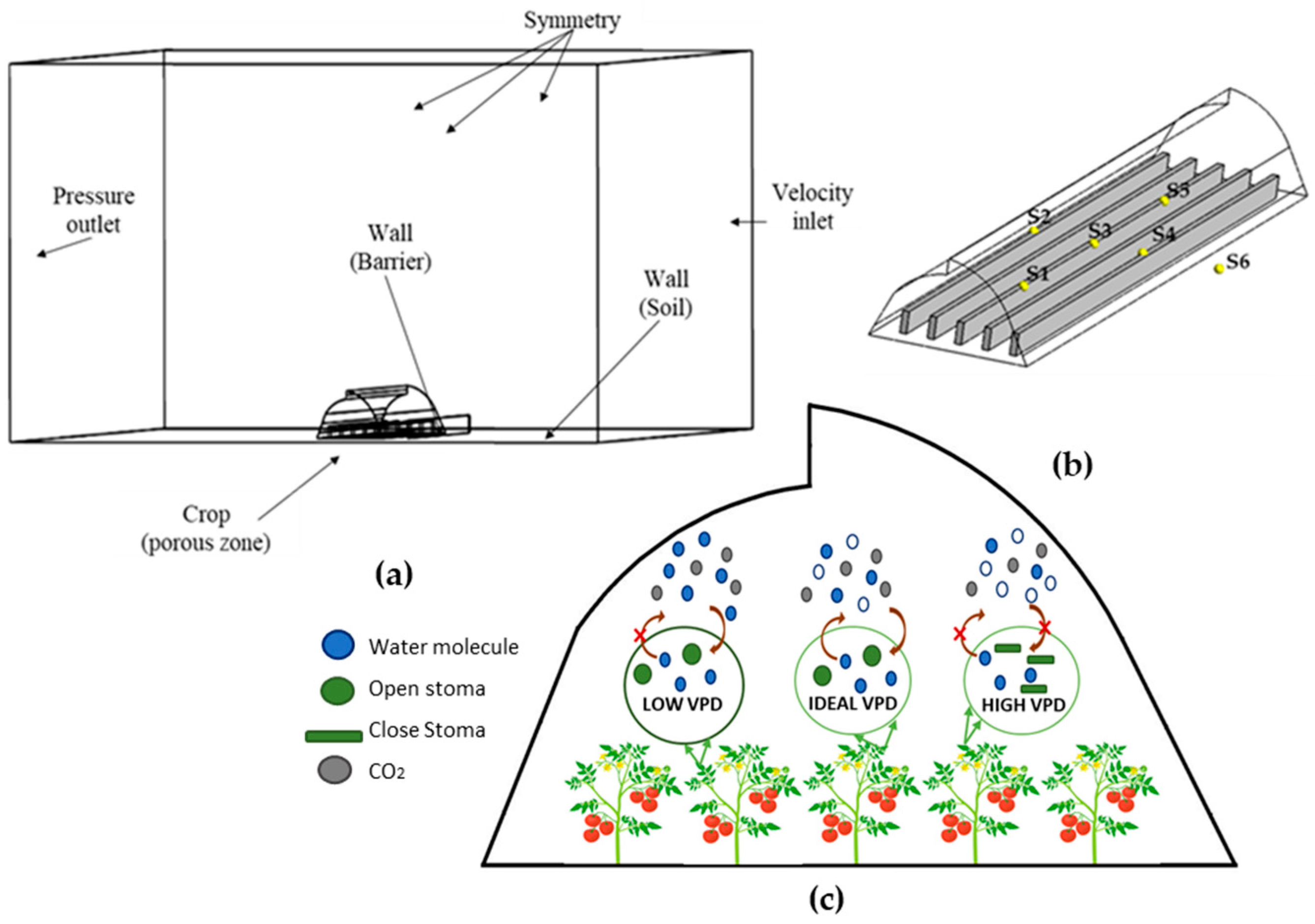
• The simulation was carried out in steady state
• A stable mass fraction was considered (ignoring crop transpiration)
• The crop was considered as a porous zone

Boundary conditions. Figure 1a: The lower part of the domain was set as soil, with the characteristics of the soil of the region. The upper part of the domain was set as a wall with a preset temperature as explained in [31,32]. The thermo-physical properties of the materials, greenhouse, soil, and crop were taken from [8,18,33].

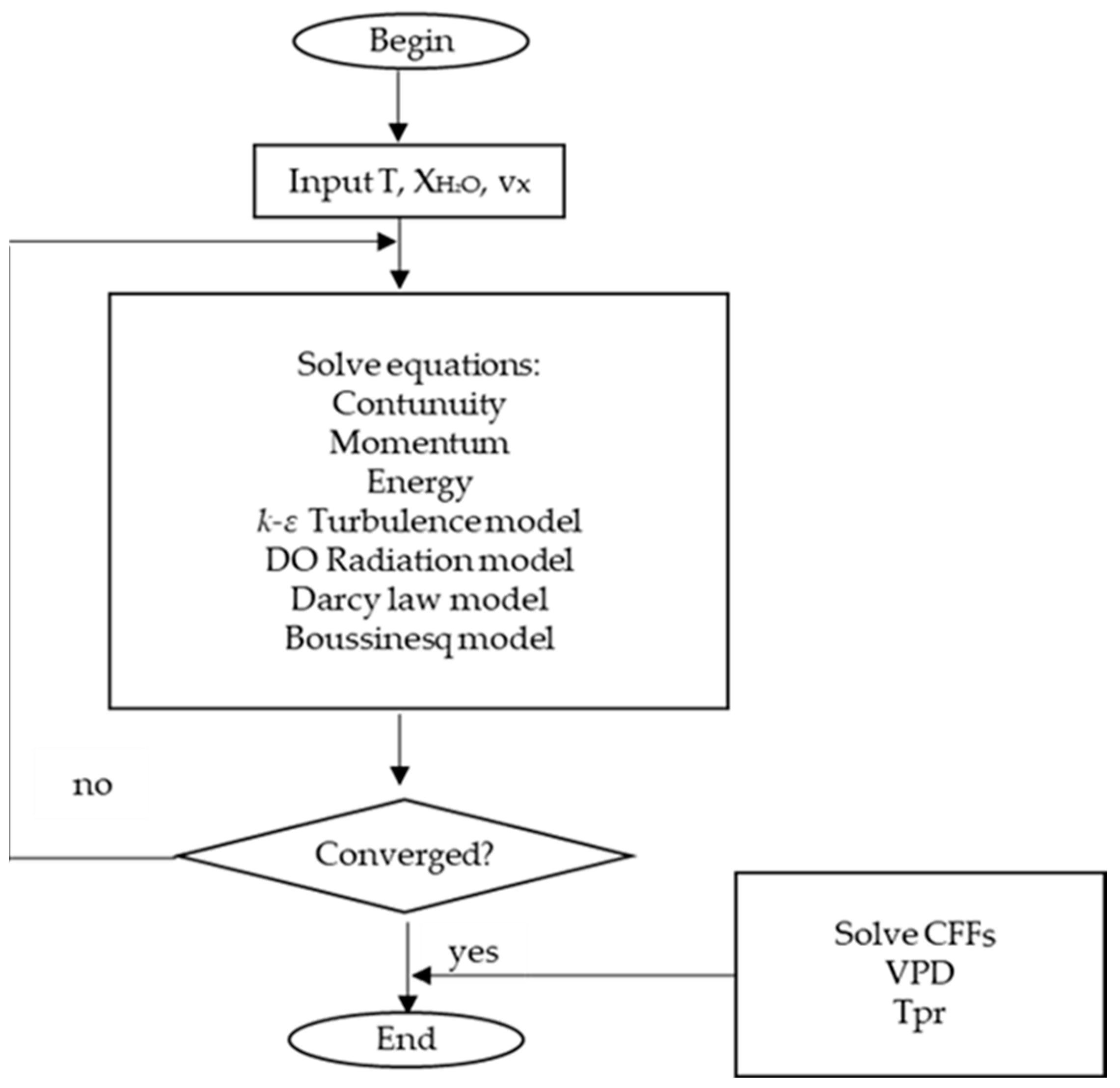
2.3. Governing Equations

The equations governing the laws of mass, momentum, and energy transport can be described by the convection-diffusion of a three-dimensional (3D) incompressible fluid at steady state by:

$${\displaystyle \frac{\rho \phi }{\partial t}}+\nabla \left(\rho \phi \overrightarrow{v}\right)=\nabla \left(\Gamma \nabla \phi \right)+S$$

(1)

where ρ is the fluid density (kg⋅m⁻³), ∇ is the nabla operator that can be applied to a scalar or a vector to represent its gradient in space, ϕ is the primary concentration variable, $\overrightarrow{v}$ is the velocity vector in m⋅s⁻¹, Γ is the diffusion coefficient in m²⋅s⁻¹, and S represents the source term [8,10].

According to the literature, the standard two-equation k—ε model is usually the most used in greenhouse simulation [1,8,26,27], and it provides favorable results. The model offers robustness, economy, and reasonable accuracy solving two equations, where the k and ε are turbulent kinetic energy, J⋅kg⁻¹, and turbulent dissipation rate, m²⋅s⁻³, respectively. Equations (2) and (3), where ${\mu }_t$ is turbulent viscosity, m²⋅s⁻¹. ${\sigma }_k$ y ${\sigma }_{\epsilon }$ are Prandtl numbers for k and ε whose values are 1.0 and 1.2, respectively. G_k and G_b represent the generation of turbulent kinetic energy due to mean velocity gradients and buoyancy, respectively. $C_{1\epsilon }$ and $C_{2\epsilon }$ are constants whose corresponding values are 1.44 and 1.9.

$${\displaystyle \frac{\partial }{\partial t}}\left(\rho k\right)+{\displaystyle \frac{\partial }{\partial x_j}}\left(\partial k{u}_j\right)={\displaystyle \frac{\partial }{\partial x_j}}\left[\left(\mu +{\displaystyle \frac{{\mu }_t}{{\sigma }_k}}\right){\displaystyle \frac{\partial k}{\partial x_j}}\right]+G_k+G_b-\rho \epsilon$$

(2)

$${\displaystyle \frac{\partial }{\partial t}}\left(\rho \epsilon \right)+{\displaystyle \frac{\partial }{\partial x_j}}\left(\sigma \epsilon u_j\right)={\displaystyle \frac{\partial }{\partial x_j}}\left[\left(\mu +{\displaystyle \frac{{\mu }_t}{{\sigma }_{\epsilon }}}\right){\displaystyle \frac{\partial \epsilon }{\partial x_j}}\right]+\rho C_{1\epsilon }S\epsilon -\rho C_{2\epsilon }{\displaystyle \frac{{\epsilon }^2}{k+\sqrt{v\epsilon }}}$$

(3)

Under night conditions, the role of radiation is often fundamental due to its impact on photosynthesis and internal microclimate; this contribution is defined as a source term in the energy equation [30]. To solve the radiative transfer equation (RTE), the Discrete Ordinate (DO) sub model, recommended for semitransparent materials [8,11,31], was solved. This model discretizes the RTE in several discrete directions in angular space by treating each direction as a vector $\overrightarrow{s}$ in the Cartesian system (x, y, z); the radiation is calculated for each of these directions, allowing a detailed analysis of how it propagates and is distributed in the medium. The DO model has provided good results in predicting the internal climate of greenhouses and is adaptable to different configurations and climatic conditions. Equation (4) shows the RTE for the spectral intensity $I_{\lambda }\left(\overrightarrow{r}, \overrightarrow{s}\right)$.

$$\nabla \left(I_{\lambda }\left(\overrightarrow{r},\overrightarrow{s}\right){\overrightarrow{s}}^{\prime }+\left({\alpha }_{\lambda }+{\alpha }_s\right)I_{\lambda }\left(\overrightarrow{r},\overrightarrow{s}\right)\right)={\alpha }_{\lambda }{n}^2{I}_{b\lambda }\left(\overrightarrow{r}\right)+{\displaystyle \frac{{\sigma }_s}{4\pi }}{\displaystyle {\int }_0^{4\pi }{I}_{\lambda }\left(\overrightarrow{r},\overrightarrow{s}\right)}\phi \left(\overrightarrow{s},{\overrightarrow{s}}^{\prime }\right)d{\Omega }^{\prime }$$

(4)

where $\overrightarrow{r}$ is the position vector, $\overrightarrow{s}$ is the direction vector, ${\overrightarrow{s}}^{\prime }$ the scattering direction vector, s the path length, $\alpha$ is the absorption coefficient, n is the refractive index, ${\sigma }_s$ the scattering coefficient, $\sigma$ the Stefan-Boltzmann constant (5.669 × 10⁻⁸ W⋅m⁻²-K⁴), I is the radiation intensity, which depends on direction and position, T the local temperature, $\Phi$ is the phase function, and Ω′ the solid angle.

The refractive index, the dispersion coefficient, and the phase function are assumed to be independent of the wavelength; they should be considered when calculating blackbody emission and semitransparent walls in their boundary conditions. The angular space is discretized in $N_{\theta }x{N}_{\varphi }$ solid angles independent of $\omega$, $\theta$ and $\varphi$, and are the polar and azimuthal angles and are measured concerning the Cartesian, polar system [34]. In this simulation, the parameters recommended by [8] were used, which provided good results without considerably increasing the computational cost.

According to previous work, the Boussinesq equation solves density differences in air caused by buoyancy effects due to low wind speeds [10,18,26].

$$\left(\rho -{\rho }_0\right)g=-{\rho }_0\beta \left(T-T_0\right)g$$

(5)

where β is the coefficient of thermal expansion, g is the force of gravity, ρ and T are the density and temperature of air with the subscript representing a reference state.

The presence of anti-insect nets was resolved using the Darcy–Forchheimer equation, which allows consideration of the pressure jump caused by the change in air velocity in the ventilation area.

$$\Delta p=-\left({\displaystyle \frac{\mu }{\alpha }}v+C_2{\displaystyle \frac{1}{2}}\rho v^2\right)\Delta J$$

(6)

where Δp is the pressure drop kg⋅m⁻¹⋅s⁻²; μ is the dynamic viscosity of the flow kg⋅m⁻¹⋅s⁻¹); where, α is the permeability of the face, m², C₂ the pressure drop coefficient, m⁻¹, and ∆J the thickness of the porous drop, m.

CFFs were included in the calculation process for the RH, VPD, and Dew point temperature, as can be seen in Figure 3. It illustrates the algorithm used to solve the models involved. First, the variables temperature, water mass fraction, and wind speed are fed. The momentum, continuity, and energy equations and the two-equation k-ε turbulence models, Darcy’s law, the Boussinesq effect, and the discrete ordinate submodel for RTE, described in the previous section, are then solved. The convergence criteria for the fluid dynamic variables were 1 × 10⁻⁶; once reached, the VPD and dew point temperature calculations were carried out. The expressions used for these calculations are shown in Equations (7) and (8)

$$PVD=0.16078\left({\displaystyle \frac{17.269\left(T\right)}{T+237.3}}\right)-\left({\displaystyle \frac{RH}{100}}\left(0.16078\left({\displaystyle \frac{17.269\left(T\right)}{T+237.3}}\right)\right)\right)$$

(7)

$$T_{dp}={\displaystyle \frac{b\left(\ln \frac{RH}{100}+\frac{aT}{b+T}\right)}{a-\ln \frac{RH}{100}+\frac{aT}{b+T}}}$$

(8)

where a and b are the coefficients of the Magnus equation [35], a = 17.625 and b = 243.04, T is the temperature, and RH the relative humidity.

2.4. Simulated Scenarios

A steady-state simulation was initially carried out for two scenarios to determine the climatic conditions at 6:00 and 18:00 h, considering the sunrise and sunset times, in order to observe possible temperature and relative humidity conditions that could generate condensation inside the greenhouse.

A simulation was then carried out taking into account the conditions of a typical day in July 2023 (day 7) and another one considering the conditions in which condensation was observed (day 27), each of them with two window opening configurations, 100% and 50%, to obtain the relationship between VPD and condensation in the state in which the greenhouse normally operates and with 100% of its ventilation capacity [36]. These simulations were carried out in steady state at 6:00 h.

Table 1. Simulated scenarios.

Scenario	Day/Window Opening Configuration
(a)	7/100%
(b)	7/50%
(c)	27/100%
(d)	27/50%

shows the simulations carried out for each scenario.

3. Results and Discussion

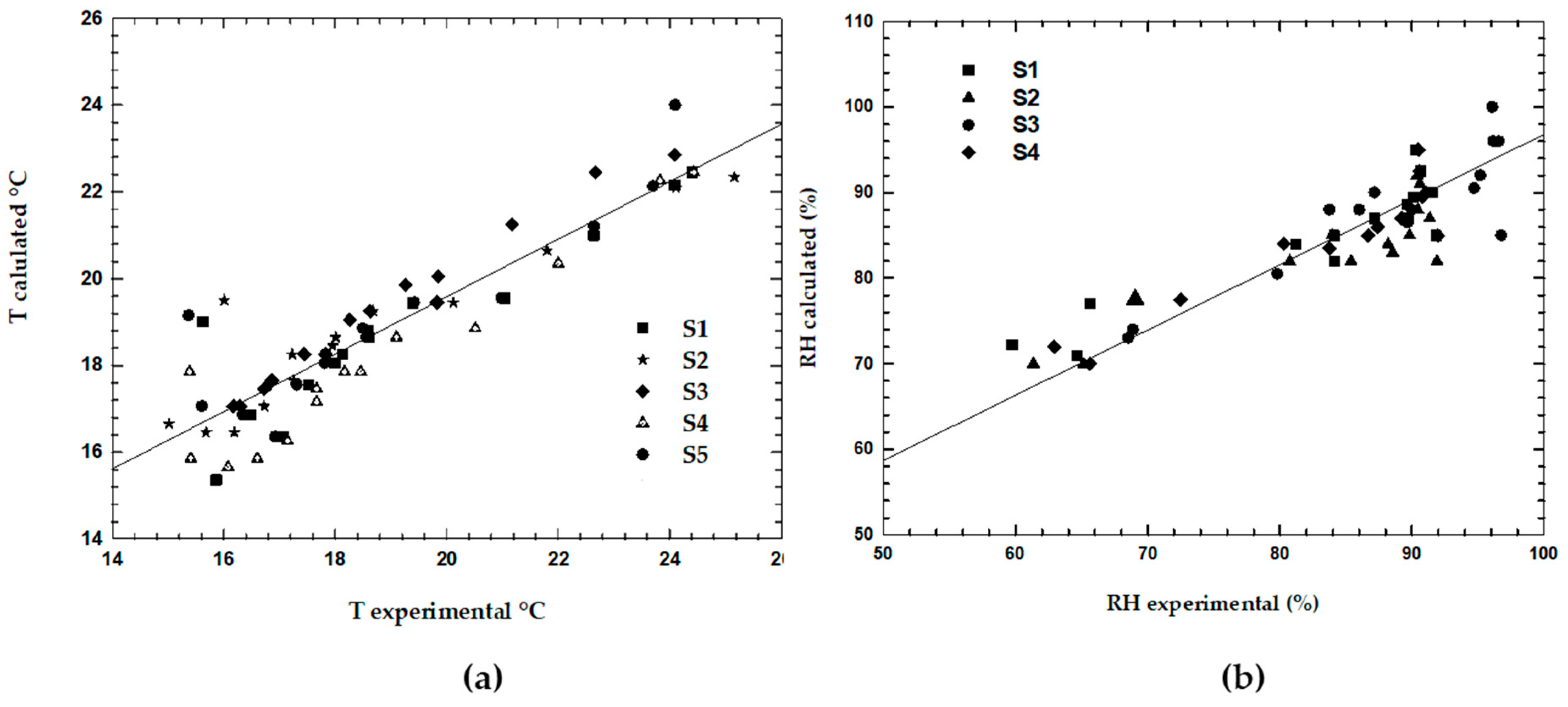
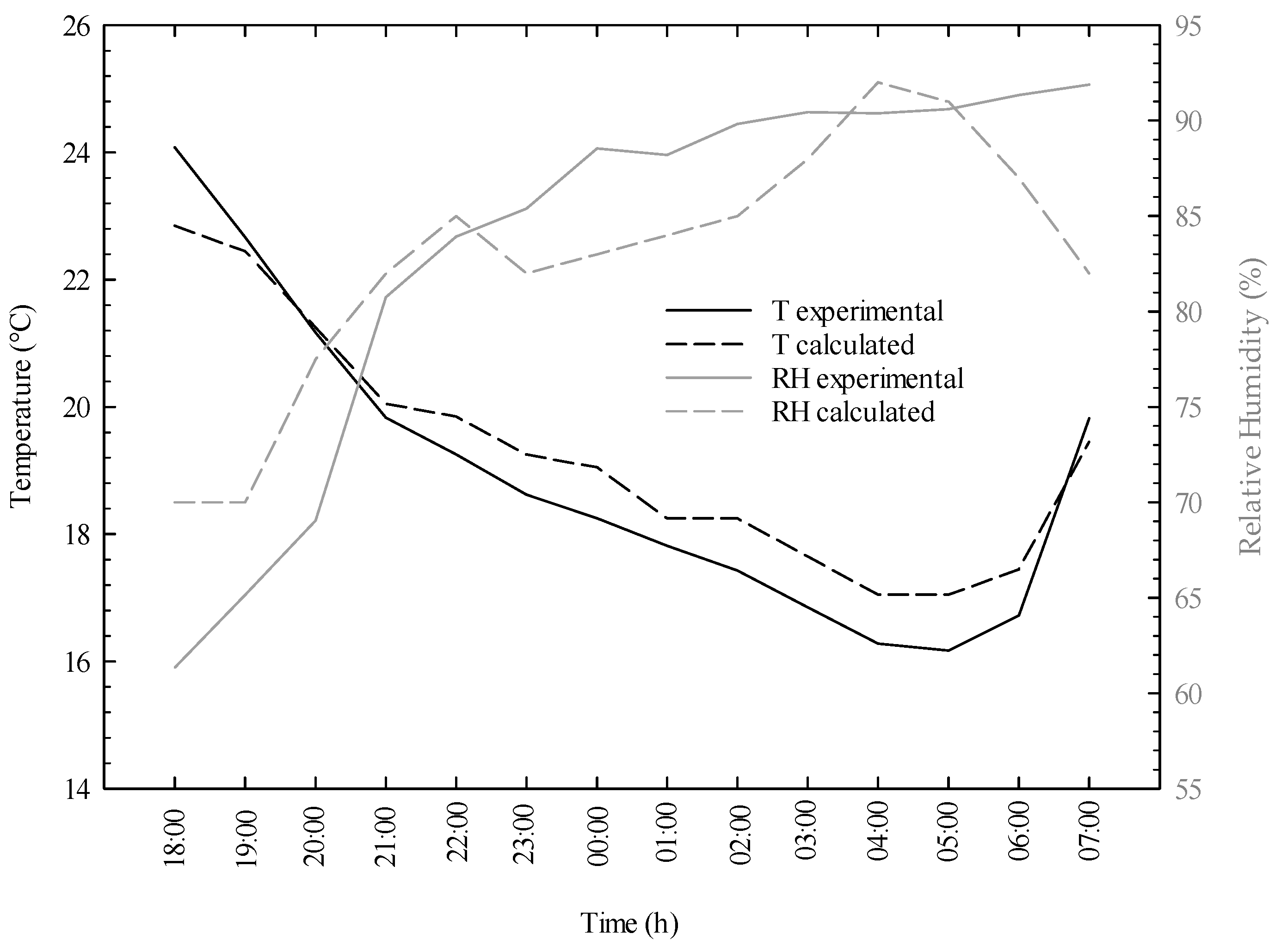
3.1. Model Validation

The model was validated using data from the night of 6–7 July 2023. The simulation was in a steady state and solved with the pressure-based approximation. Temperature and relative humidity data were recorded every 10 min and averaged hourly. The mean square error and R² were used as fitting models. The initial conditions used were the external temperature, relative humidity, and wind speed, which are the variables of the environment outside the greenhouse. The sky temperature was calculated according to [31]. Figure 4 shows the comparisons between the experimental measurements and the results obtained by the numerical model for the variables of temperature and relative humidity, RH, identified as Figure 4a and Figure 4b, respectively, for five sensors distributed in the greenhouse. Both Temperature and Relative Humidity are within a 16% and 17% error range, respectively, which allows us to determine that the calculated values are very close to the actual greenhouse operation. Notably, the most significant difference is obtained at low temperatures and higher relative humidity, obtaining coefficients of determination of 0.84 and 0.83 for temperature and relative humidity, respectively, and RMSE of 1.1 and 4.2, agreeing with statistical data previously reported by [8,10,26].

On the other hand, Figure 5 shows the temperature and relative humidity data, respectively, as a function of time, with the behavior being appreciated in a range of 13 h. The temperature data between the experimental and calculated measurements are very close to each other, which determines that the model correctly solves the phenomena involved. In the case of relative humidity, a greater difference was obtained between both models in the first hours and at the end of the day, and this is because this model does not consider the sources of water vapor (soil and crops); it is based on the established external relative humidity. Another source of error is the stable state solution. However, with this, we seek to obtain a computationally more accessible model with acceptable results.

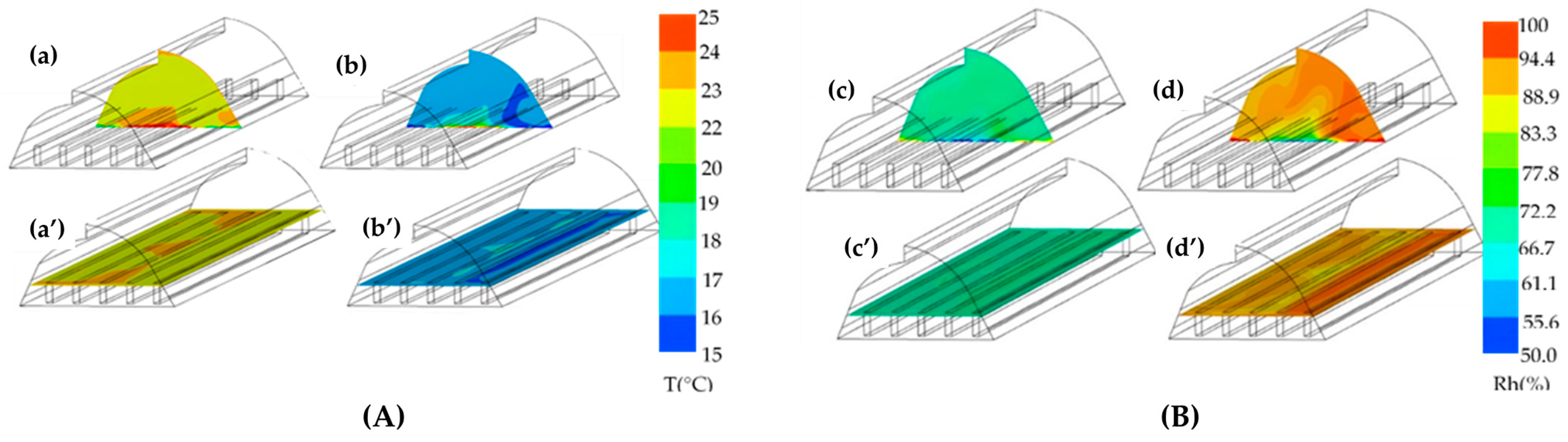
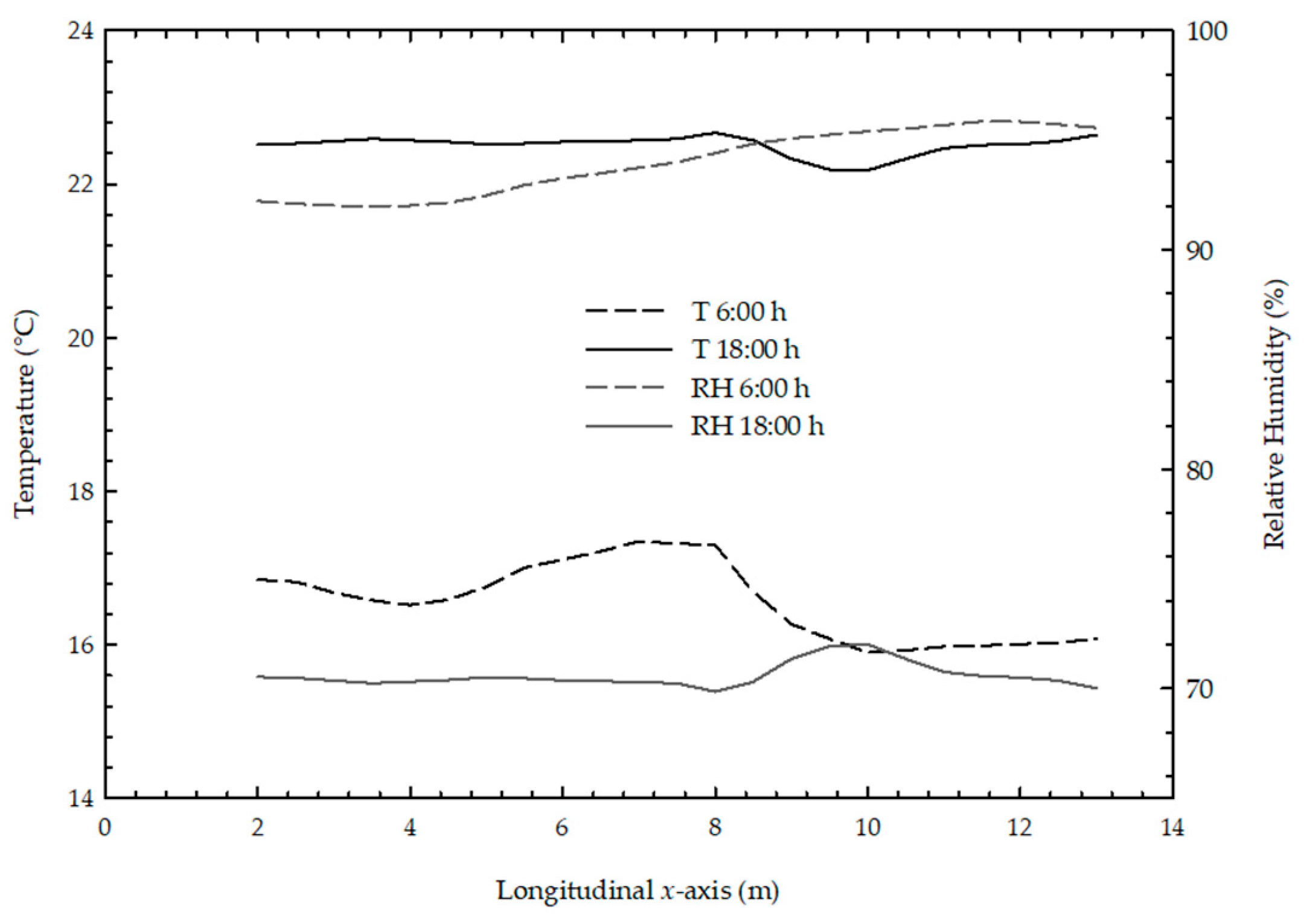
3.2. Simulation 6:00 and 18:00 h

Figure 6A,B show the temperature and relative humidity profiles, respectively, in two planes of the greenhouse; a, b shows a transversal profile in the middle of the greenhouse and a’, b’ a longitudinal plane parallel to the ground two meters from it, corresponding to the height of the canopy. These results were obtained for the study cases with 50% windows opening at 18:00 h, beginning of sunset, and at 6:00 h, sunrise, respectively. In the evening, Figure 6a,a’ the temperature oscillates between 22 and 23 °C, and the highest is located at the center of the greenhouse. In the case of morning temperatures, Figure 6b,b’ the behavior of the thermal field shows temperature ranges between 16 and 17.5 °C with higher temperatures recorded at the center, and lower near the ventilation inlets. In the case of relative humidity profiles shown in Figure 6B, the results are opposite to those obtained for temperature in Figure 6c,6c’ for 18:00 hrs and Figure 6d,6d’ for 6:00 h. In the evening profiles, the humidity maintains a homogeneous value in most of the greenhouse, which at 18:00 h is close to 70% with a slight rise near the right window. In Figure 6d,d’, the RH values increase near the windows, fluctuating between 94% in the right window and 87% in the center, and increasing as it moves toward the left wall to reach 90%. It is observed that the temperature and relative humidity values in the afternoon do not reach critical values that indicate a risk of condensation because, although the sun is setting at the simulated time, there are still remnants of the high temperature reached during the day; this causes the relative humidity values to remain at levels suitable for the crop. The values denoted by the color patterns are notably reversed in the afternoon and morning, with high temperatures and low relative humidity at 6:00 p.m. and low temperatures and relative humidity values close to 95% at 6:00 a.m. Since the crop transpires at night, the air becomes saturated with humidity, and a sudden temperature change can generate conditions for condensation to occur with a greater probability at that time, where the lowest temperature values were recorded within the time range studied. Figure 7 shows the temperature and relative humidity graphs for 6:00 p.m. and 6:00 a.m. using a vertical profile located at 40 m in the z-direction (middle of the greenhouse) and a horizontal profile at two meters high. The high humidity levels observed at dawn on 7 July, combined with low temperatures, provide a greater risk of condensation [26,27].

Figure 8 shows the correlations of VPD with temperature and relative humidity using the simulated data for 6:00 a.m. on 7 July 2023. The VPD shows a strong positive correlation with temperature and an inversely proportional behavior with relative humidity [18]. It is observed that the VPD values are below 0.3, with a predominantly humid environment with a change of 10 percentage points on the scale, while the temperature only varies by approximately 2 °C. Both R² values were 0.99.

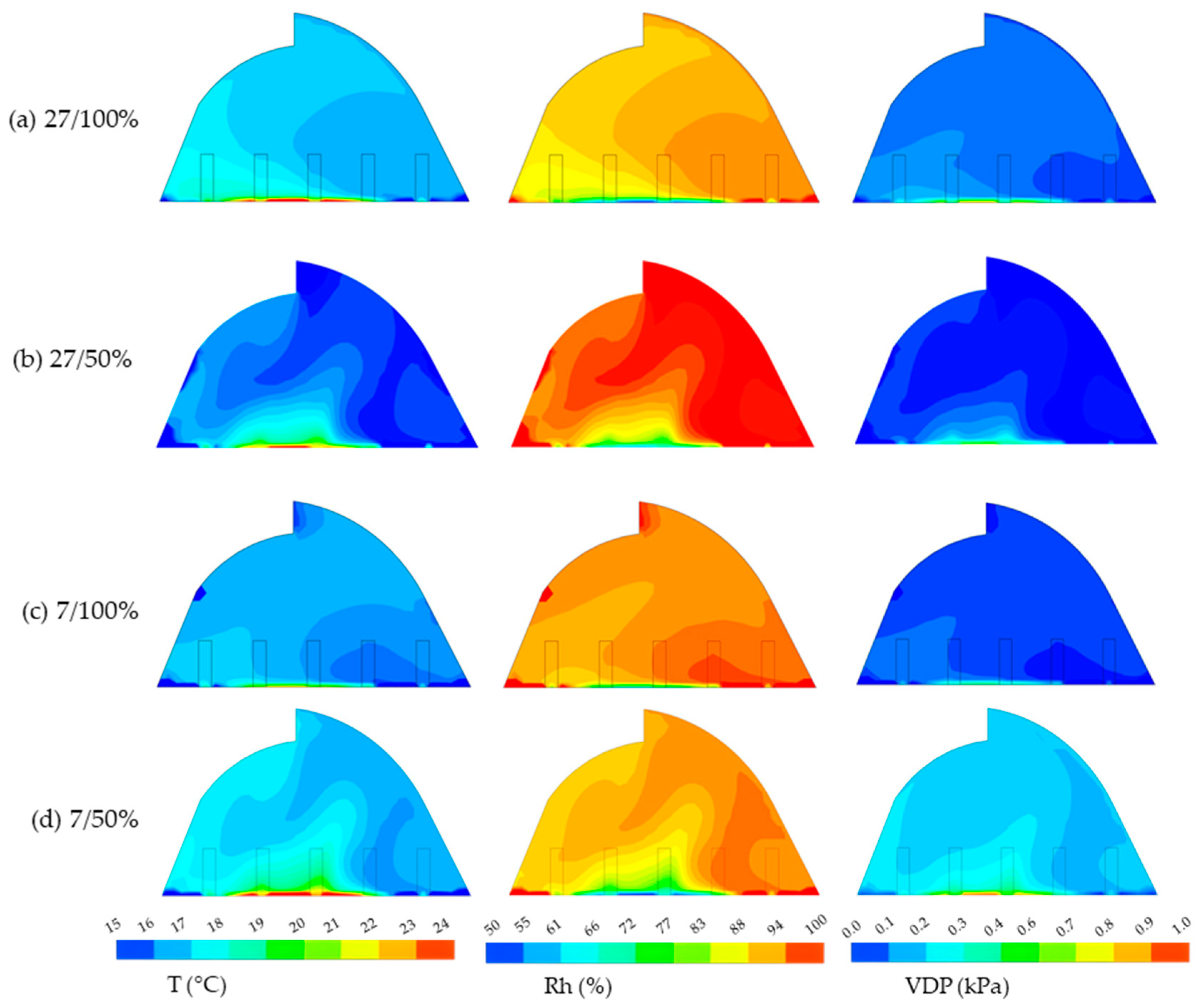
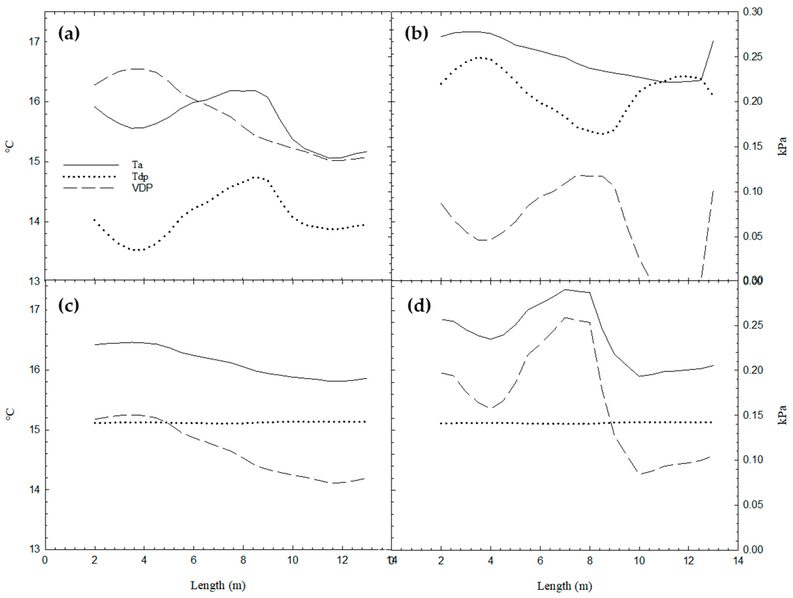
3.3. Simulation Scenarios

From these results, four scenarios were evaluated to analyze the relationship between VPD and condensation through the dew point. The calculation is performed by subtracting the dew point temperature from the ambient temperature. When values equal to or less than zero are obtained, condensation conditions are considered. A simulation was conducted with data from July 7 (validation) and 27 of the same month, where condensation was observed inside the greenhouse on the second day mentioned. The behaviors of temperature, relative humidity, and VPD were compared for each case, with whole opening (100%) and partial opening (50%) of the windows for nights with condensation and typical weather.

Figure 9 shows the obtained temperature, relative humidity, and VPD profiles in both the 100% opening model and the 50% opening on both days. The VPD is below 0.35 kPa, indicating that plant transpiration has been reduced and there are conditions for establishing fungal and bacterial diseases [10]. Figure 9a,b correspond to the experimental conditions of localized condensation, mainly on the right side of the greenhouse, where most of the humidity is concentrated and the temperature is lower. The high humidity values observed at dawn on 27 July, combined with low temperatures, provide a greater risk of condensation, which coincides with that reported by Baxevanou et al., and Lu et al. [26,27]. Temperatures between 15 and 16 °C are observed for the open greenhouse, and relative humidity of 90–95%, which results in VPD values between 0.13 and 0.23, while for the 50% opening, temperatures of 16 to 17 °C and humidity of 95–100% are observed, and the VPD drops to 0.001–0.13. In this case, a dew point is reached that equals the ambient temperature, which generates condensation. What is described at this point is the beginning of condensation, or what Piscia et al. [11] call the start phase. The behavior of the temperature, RH, and VPD variables coincide with those reported by Aguilar Rodríguez et al. [18], who conducted a daytime study for the central part of a three-span greenhouse. Humidity values of 100% and a dew point temperature greater than or equal to the ambient temperature correspond to VPD values equal to zero.

For Figure 9c,d that correspond to open and semi-open windows of a typical night, the profiles show a temperature between 15 and 16 °C for the open greenhouse, and a decrease in relative humidity is observed concerning Figure 9d with values of 92–95% and VPD of 0.07–0.14 kPa. When the windows are opened at 50%, the temperature increases to a range of 16–17 °C, with a relative humidity of 87–96%, and the VPD ranges from 0.08–0.25 kPa, keeping the ambient temperature above the dew point temperature. However, these VPD values can endanger the plants, so an emergency heating system is necessary to raise the temperature and control humidity, as reported by Villagran et al. and Tamimi et al. [10,24].

Figure 10 shows the graphs of the data obtained on 27 July 2023, at 6:00 a.m. (experimental condensation) for an open and semi-open greenhouse and the corresponding ones obtained on 7 July at 6:00 a.m. to analyze the behavior of the VPD concerning ambient temperature (T_a), and dew point temperature (T_dp). Figure 10a shows the simulated behavior for a day with condensation at 100% opening, where the differences between T_dp and T_a remain above 1 °C, a decrease in T_dp is observed caused by the decrease in relative humidity and T_a caused by air renewal by increasing the ventilation area, thus the VPD values are 0.1–0.3; in this case the simulation indicates that condensation can be avoided. In Figure 10b, with a 50% opening in the ventilation, it can be seen along the x-axis (greenhouse width) how the values of T_dp and T_a are closer; the decrease between the differences of these variables causes a decrease also in the VPD values. The main condensation conditions are shown on the right side of the graph, which coincides with the air inlet to the greenhouse, where the difference between T_dp and T_a becomes negative at these points, and the VPD falls to zero as well. The VPD values increase proportionally to the difference between T_a and T_dp. This behavior can also be seen in Figure 10a. In Figure 10, when the windows are opened to 100%, a slight decrease in T_a is observed, which causes a drop in the VPD values with the closeness between the values of Ta and T_dp for those presented in Figure 10d where there is a 50% opening of the windows for the day where condensation does not occur. The VPD behavior follows the trends described for Figure 10a,b regarding the difference between Ta and T_dp. On this day, the T_dp values remain quasi-constant, and the VPD behavior varies proportionally from the T_a. The fluctuations in the behavior of the variables are more noticeable in Figure 10a,b, where it is observed that when opening the windows to 100%, the VPD maintains values between 0.15 and 0.25. The dew point remains below the ambient temperature by up to 2 °C; however, when opening to 50%, T_dp reaches values higher than Ta and the VPD values of 0, thus showing the presence of condensation. In the case of Figure 10c,d, the T_dp values remain constant regardless of the opening of the windows. The VPD behaves proportional to T_a with higher values in Figure 10d. In both cases, the value decreases as it approaches the right end of the graph, indicating the greenhouse ventilation inlet.

4. Conclusions

A numerical simulation of a naturally ventilated Gothic-type greenhouse used in semi-desert areas of northern Mexico for tomato cultivation was developed. The conditions of temperature, relative humidity (RH), and their influence on the VPD at critical times were analyzed to determine if they can be used as an indicator of risk or presence of condensation, reaching the following conclusions:

• The time with the highest risk of condensation is 6:00 a.m., with humidity levels of up to 97%. At dusk, humidity levels are not high enough to generate conditions for this phenomenon since they are below 75%.
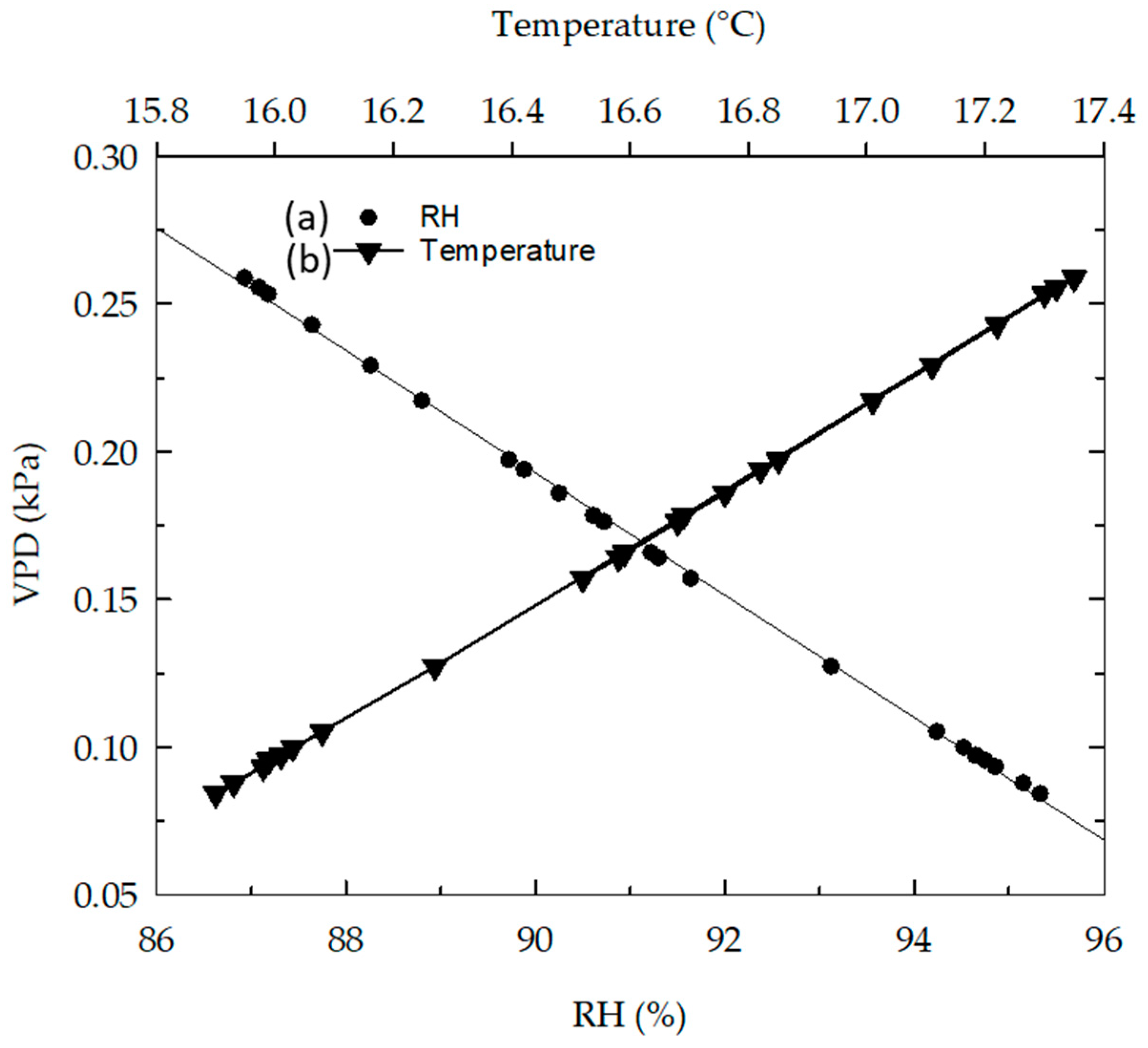
• The VPD can be used as an indicator of the presence of condensation inside the greenhouse. As its value approaches zero, the probability of condensation increases. The risk of condensation is seen from values less than 0.1 kPa.
• The dew point temperature can be considered as an alternative to determine the risk of condensation by analyzing the behavior of the difference between its values and those of the ambient temperature.
• Under the simulated conditions, fully opening the windows can prevent the VPD from reaching zero and, therefore, condensation. Timely opening of the windows can also help decrease the relative humidity and increase the difference between ambient temperature and T_dp.

As future work, it is recommended to develop more robust VPD and condensation models, including variables such as crop transpiration, and to develop the solution in a transient model.

References

1. Velázquez, J.F.; Saenz, E.M.; Camacho, J.I.M.; Rojano, A. Análisis numérico del clima interior en un invernadero de tres naves con ventilación mecánica. Agrociencia 2011, 45, 545–560. [Google Scholar]
2. Fatnassi, H.; Boulard, T.; Benamara, H.; Roy, J.; Suay, R.; Poncet, C. Increasing the height and multiplying the number of spans of greenhouse: How far can we go? Acta Hortic. 2017, 1170, 137–144. [Google Scholar] [CrossRef]
3. Villagran, E.A.; Bojaca, C. Numerical evaluation of passive strategies for nocturnal climate optimization in a greenhouse designed for rose production (Rosa spp.). Ornam. Hortic. 2019, 25, 351–364. [Google Scholar] [CrossRef]
4. López, A.; Valera, D.L.; Molina Aiz, F. Sonic anemometry to measure natural ventilation in greenhouses. Sensors 2011, 11, 9820–9838. [Google Scholar] [CrossRef] [PubMed]
5. Rocha Ortiz, G.A.; Pichimata, M.A.; Villagran, E. Research on the Microclimate of Protected Agriculture Structures Using Numerical Simulation Tools: A Technical and Bibliometric Analysis as a Contribution to the Sustainability of Under-Cover Cropping in Tropical and Subtropical Countries. Sustain. Sci. 2021, 13, 10433. [Google Scholar] [CrossRef]
6. Tong, G.; Christopher, D.M.; Li, B. Numerical modelling of temperature variations in a Chinese solar greenhouse. Comput. Electron. Agric. 2009, 68, 129–139. [Google Scholar] [CrossRef]
7. Fitz Rodriguez, E.; Kubota, C.; Giacomelli, G.A.; Tignor, M.E.; Wilson, S.B.; McMahon, M. Dynamic modeling and simulation of greenhouse environments under several. Comput Electron Agric. 2010, 70, 105–116. [Google Scholar] [CrossRef]
8. Piscia, D.; Montero, J.I.; Baeza, E.; Baely, B.J. Un modelo CFD de condensación nocturna en invernadero. Ing. Biosist. 2012, 111, 141–154. [Google Scholar]
9. Willits, D.H.; Peet, M.M. El efecto de la temperatura nocturna sobre los rendimientos de tomates cultivados en invernadero en climas cálidos. Agric. Meteorol. 1998, 92, 191–202. [Google Scholar] [CrossRef]
10. Villagran Munar, E.A.; Bojaca Aldana, C.R. Simulación de microclima en un invernadero utilizado para la producción de rosas en condiciones de clima intertropical. Chil. J. Agric. Anim. Sci. 2019, 35, 137–150. [Google Scholar] [CrossRef]
11. Piscia, D.; Flores, J.; Montero, J. Predicting nocturnal condensation in a multi-span greenhouse using computational fluid dynamics simulations. Acta Hortic. 2010, 927, 627–634. [Google Scholar] [CrossRef]
12. Díaz Rodriguez, A. Métodos de Predicción y Técnicas de Control de la Condensación en Invernaderos. Ph.D. Thesis, Universidad Politécnica de Madrid, Madrid, Spain, 2009. [Google Scholar] [CrossRef]
13. Bounet, P.E. Assessing greenhouse climate using CFD: A focus on air humidity issues, International Symposium on New Technologies for Environment Control, Energy-Saving and Crop Production in Greenhouse and Plant. Acta Hortic. 2014, 1037, 971–985. [Google Scholar] [CrossRef]
14. Leal, I.; Alcorta García, E.; Rodriguez Fuentes, H. Modelado del clima en invernaderos. Ingenierías 2006, 9, 7–13. [Google Scholar]
15. Both, A.J.; Franklin, J.; Benjamin, L.; Holroyd, G.; Incoll, L.D.; Lefsrud, M.G.; Pitkin, G. Guidelines for measuring and reporting environmental parameters for experiments in greenhouses. Plant Methods 2015, 11, 43. [Google Scholar] [CrossRef] [PubMed]
16. Baptista, F.J.; Bailey, B.J.; Meneses, J.F. Effect of nocturnal ventilation on the occurrence of Botrytis cinerea in Mediterranean unheated tomato greenhouses. Crop Prot. 2012, 32, 144–149. [Google Scholar] [CrossRef]
17. Huertas, L. El control ambiental en invernaderos: Humedad relativa. Horticultura 2008, 205, 52–54. [Google Scholar]
18. Aguilar Rodriguez, C.E.; Flores Velazquez, J.; Rojano, F.; Flores Magdaleno, H.; Rubiños Panta, E. Simulation of Water Vapor and Near Infrared Radiation to Predict Vapor Pressure Deficit in a Greenhouse Using CFD. Processes 2021, 9, 1587. [Google Scholar] [CrossRef]
19. Cuellar Murcia, C.A.; Suarez Salazar, J.C. Sap flow and water potential in tomato plants (Solanum lycopersicum L.) under greenhouse conditions. Rev. Colom. Cienc. Hortícolas 2018, 12, 104–112. [Google Scholar] [CrossRef]
20. Zhang, D.; Du, Q.; Zhang, Z.; Xiaocong, J.; Song, X.; Li, J. Vapour pressure deficit control in relation to water transport and water productivity in greenhouse tomato production during summer. Sci. Rep. 2017, 7, 43461. [Google Scholar] [CrossRef]
21. Rivano, F.; Jara, J. Estimación de la evapotranspiración de referencia en la localidad de Remehue-Osorno, X región. Agro Sur. 2005, 33, 49–61. [Google Scholar] [CrossRef]
22. BioAgro Tecnologies. Available online: https://brioagro.es/dpv-deficit-de-presion-de-vapor/ (accessed on 26 June 2024).
23. Luo, W.; Goudriaan, J. Dew formation on rice under varying durations of nocturnal radiative loss. Agric. Meteorol. 2000, 104, 303–313. [Google Scholar] [CrossRef]
24. Lu, N.; Kamimura, N.; Taichi, K.; Dalong, Z.; Ikusaburo, K.; Michiko, T.; Toru, M.; Toyoki, K.; Wataru, Y. Control of vapor pressure deficit (VPD) in greenhouse enhancedtomato growth and productivity during the winter season. Sci. Hortic. 2015, 197, 17–23. [Google Scholar] [CrossRef]
25. Tamimi, E.; Kacira, M.; Choi, C.Y.; An, L. Analysis of microclimate uniformity in a naturally vented greenhouse with a high-pressure fogging system. Trans. ASABE 2013, 56, 1241–1254. [Google Scholar] [CrossRef]
26. Villagran, E.; Flores Velázquez, J.; Mohamed, A.; Bojaca, C. Influencia de la altura en un invernadero multitúnel colombiano en la ventilación natural y el comportamiento térmico: Enfoque de modelación. Sustain. Sci. 2021, 13, 136331. [Google Scholar] [CrossRef]
27. Baxevanou, C.; Fidardos, D.; Bartzanas, T.; Kittas, C. Numerical simulation of solar radiation, air flow and temperature. Ing. Agrícola Int. CIGR J. 2010, 12, 48–67. [Google Scholar]
28. Li, A.; Huang, L.; Zhang, T. Field test and analysis of microclimate in naturally ventilated single-sloped greenhouses. Energy Build 2017, 138, 479–489. [Google Scholar] [CrossRef]
29. Slatni, Y.; Djezzar, M.; Messai, T.; Brahim, M. Numerical simulation of thermal behavior in a naturally ventilated greenhouse. Int. J. Comput. Sci. Eng. 2022, 11, 2150034. [Google Scholar] [CrossRef]
30. Bouhoun, A.H.; Bournet, P.E.; Danjou, V.; Migeon, C. CFD analysis of the climate inside a closed greenhouse at night including condensation and crop transpiration. Acta Hortic. 2015, 1170, 53–60. [Google Scholar] [CrossRef]
31. Montero, J.I.; Muñoz, P.; Sánchez Gerrero, M.C.; Medrano, E.; Piscia, D.; Lorenzo, E. Shading screens for the improvement of the night-time climate of unheated greenhouses. Span. J. Agric. Res. 2013, 11, 32–46. [Google Scholar] [CrossRef]
32. Iglesias, N.; Montero, J.I.; Muñoz, P.; Antón, A. Estudio del clima nocturno y el empleo de doble cubierta de techo como alternativa pasiva para aumentar la temperatura nocturna de los invernaderos utilizando un modelo basado en la Mecánica de Fluidos Computacional (CFD). Hort. Argent. 2009, 28, 18–23. [Google Scholar]
33. Fidardos, D.K.; Bexevanou, C.A.; Bartzanas, T.; Kittas, C. Numerical simulation of thermal behavior of a ventilated arc greenhouse during a solar day. Renew. Energy 2010, 35, 1380–1386. [Google Scholar] [CrossRef]
34. Fidardos, D.; Kittas, C.; Baxevanou, C.; Bartzanas, T. Solar radiation distribution in a tunnel greenhouse. Acta Hortic. 2008, 801, 855–862. [Google Scholar] [CrossRef]
35. Alduchov, O.A.; Eskridge, R. Improved Magnus form approximation of saturation vapor pressure. J. Appl. Meteorol. 1996, 601–609. [Google Scholar] [CrossRef]
36. Marquez Vera, M.A.; Ramos Fernandez, J.C.; Cerecero Natale, L.F.; Lafont, F.; Balmat, J.F.; Esparza Villanueva, J.I. Temperature control in a MISO greenhouse by inverting its fuzzy model. Comput. Electron. Agric. 2016, 124, 168–174. [Google Scholar] [CrossRef]
Figure 1. (a) Computational domain and boundary conditions, (b) Greenhouse geometry and sensor location, (c) VPD in greenhouse.
Sustainability 17 01957 g001
Figure 2. Mesh sensitivity analysis.
Sustainability 17 01957 g002
Figure 3. Process diagram for CFFs.
Sustainability 17 01957 g003
Figure 4. Linear regression by sensor for (a) Temperature and (b) Relative Humidity.
Sustainability 17 01957 g004
Figure 5. Experimental vs. calculated Temperature and Relative Humidity.
Sustainability 17 01957 g005
Figure 6. (A) Temperature profiles (a,a’) 18:00 h and (b,b’) 6:00 h. (B) Relative humidity profiles (c,c’) 18:00 h and (d,d’) 6:00 h.
Sustainability 17 01957 g006
Figure 7. Behavior of Temperature and RH at 6:00 a.m. and 6:00 p.m.
Sustainability 17 01957 g007
Figure 8. Linear regression of VPD vs. (a) Relative Humidity, (b) Temperature.
Sustainability 17 01957 g008
Figure 9. T, RH, VPD profiles with different days and percentages of window openings (a) 27/100% (b) 27/50% (c) 7/100% (d) 7/50%.
Sustainability 17 01957 g009
Figure 10. (a) 27/100%, (b) 27/50% (c) 7/100% (d) 7/50%.
Sustainability 17 01957 g010