Abstract
Shallow lakes are important drinking water sources, but are easily affected by wind. Turbidity is an indicator that fluctuates dramatically with changes in wind and is affected not only by the instantaneous wind speed but also by the wind direction, duration, etc. The Weibull distribution was introduced to describe the distributions of the wind conditions and turbidity during a seasonal period. The relationship between the mean wind-power density and the corresponding turbidity reached 0.8, which showed a relatively strong correlation. A turbidity prediction model was built by the random forest algorithm and was fed with the mean wind-power density and temperature. The results indicated that nearly half of the test samples had REs less than 20%, which was enough for waterworks to adjust the dosage in advance. The findings can be used to develop turbidity prediction models using meteorological forecast data and provide a reference for waterworks with shallow lakes as sources.
1. Introduction
Turbidity is a crucial index for evaluating the quality of drinking water in terms of the degree of obstruction when light passes through a solution. This phenomenon is closely related to the contents of impurities, such as sediment, clay, plankton, and microorganisms [1]. The sediment suspension and migration induced by wind disturbances have become significant factors influencing turbidity variation in shallow water bodies [2], which are characterized by open water—sediment interfaces and shallow depths. Rapid fluctuations in raw water turbidity directly affect the operational performance of waterworks with large shallow lakes as supplies [3]. Therefore, research on the influence of wind on turbidity fluctuations has become more popular in recent years, with the aim of establishing an effective strategy to forecast and analyze the turbidity of drinking water sources in advance and to optimize process parameters for waterworks in a timely manner.
As wind is absorbed into a water body via energy, the bottom shear stress caused by wind-induced waves is believed to be the crucial factor for sediment suspension, and wave-induced flow also affects the hydrodynamic environment of shallow lakes [4,5]. The turbidity variation is related not only to the instantaneous wind but also to the joint probability distributions of the wind speed and direction in a given period and location. A mathematical model of sediment suspension and transportation that considers wave effects was first proposed and verified in several typical shallow water bodies, such as Lake Okeechobee in the USA [6], Boyang Lake [7] and Lake Taihu in China [2]. The critical wind speed and shear stress resulting in sediment suspension have also been determined through measurement analysis [8,9], a physical model [10], and a theoretical formula [11,12].
To quantify the response of turbidity to the wind field, a regression model based on wind data has been established to explore the linear or nonlinear relationship with turbidity [13,14]. The optimized regression model still fails to reach the required accuracy because it is unable to solve nonlinear problems effectively. With the development of artificial intelligence, machine learning models have been more widely applied to water quality prediction [15,16,17,18] because of their superior ability to address the complex nonlinear characteristics of water environment systems. The input variables include not only the wind speed and direction but also other indices, such as the dissolved oxygen concentration, pH, conductivity and chlorophyll a concentration. This increases the model accuracy but ignores the difficulty of the acquisition of these water quality indicators and limits its practical application.
In recent years, numerical simulations using various software, such as MIKE3, EFDC, FVCOM, Delft-3D, and ECOMSED, have been widely adopted, and multiple processes influenced by wind, such as sediment suspension, transportation and sedimentation, have been simulated. Although the conversion relationship between turbidity and suspended sediment has been proven in some shallow water bodies, especially those whose hydrodynamics are mainly controlled by wind, studies on the direct relationship between turbidity and wind conditions are less common.
In general, previous studies have focused more on the effects of ambient wind conditions on the suspended sediment of shallow lakes, but fewer researchers have focused on the problem of turbidity. Previous studies have been conducted to determine the relationship between turbidity variations and wind conditions through synchronized data but have rarely considered the distribution pattern over a long period. Thus, the short-term prediction of turbidity has been the focus of research, but the results have been less effective for the emergency management of waterworks. To address this problem, a waterworks with Lake Taihu as its source was selected as a case study. The recorded high-frequency turbidity data of raw water and wind data of the water intake area were collected in the current study to (1) describe the seasonal characteristics of the distribution of wind conditions by using the Weibull distribution function, as well as turbidity fluctuations; (2) perform quantitative analysis of the correlation between the wind distribution and turbidity fluctuations from the perspective of seasonal division by using the parameter of wind power density; and (3) build a prediction model of turbidity by considering the effect of the wind field and its duration on turbidity. The model found in this study achieved medium-term forecasts with only temperature and wind data as inputs. This helps the water workers adjust the dosage in advance, which further contributes to cost control and emergency management. The roadmap is as Figure 1:
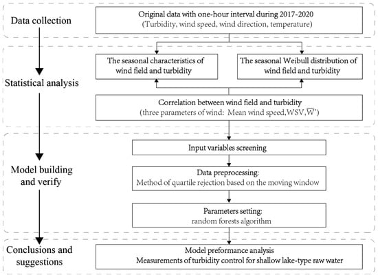
Figure 1.
Roadmap.
2. Materials and Methods
2.1. Data Sources
Lake Taihu (30°56′~31°33′ N and 119°53′~120°36′ E), located in the lower Yangtze Delta, is the third largest freshwater lake in China. It is also a typical shallow lake with a large water surface area of 2388.1 km2 and a mean depth of 1.9 m (Figure 2a). Further, the maximum depth is less than 2.6 m also. The average annual runoff from the lake is about 7.5 billion cubic meters with a water storage of 4.4 billion cubic meters. The lake has become an important drinking water source for 38 cities around and approximately 60 million people [3]. The city of Huzhou, Zhejiang Province, with Lake Taihu to the north, is one of the beneficiaries, and waterworks A located there (Figure 2b, from Baidu map) was selected as the observation object in this study. Raw water is pumped from eastern Lake Taihu to the waterworks through two 7.6 km long diversion pipes. The average water depth of the intake area is only approximately 1 m and is close to the bank. The shallowness and large water—soil contact area make it easier for wind-induced waves and currents to cause intense hydrodynamic disturbances in the water body [19,20], thus agitating the sediment and causing dramatic fluctuations in the influent turbidity of the waterworks.
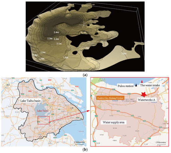
Figure 2.
(a) The bathymetry map and (b) the locations of waterworks A.
The 10 min average wind speed and direction data used in this study were from the Pulou meteorological station (30°56′00′′ N, 120°17′57′′ E), which is closest to the water intake, and were collected by the Huzhou Meteorological Observatory of Zhejiang Province at an interval of 1 h. The historical turbidity data were provided by waterworks A. The water intake is about 70 m from the shore, and the depth is 0.5 m underwater. The water is pumped from the intake and transported to the waterworks through two 7.6 km long pipes. The turbidity values were acquired by a Hach online turbidity meter installed in the waterworks inlet with an interval of 1 h. The turbidity of the raw water was also measured manually by the staff three times a day (9:00, 15:00, 21:00) in the laboratory. By comparing the samples of two months, the relative error between the automatic monitoring data and the manual data is less than 15%. The precision is sufficient to execute the data analysis afterwards. The recorded meteorological and turbidity data used were from 1 January 2017 to 31 December 2020.
2.2. Weibull Distribution Function
In 1989, Dargah-i Noubari [21] generalized three patterns that could describe the distribution of the wind speed well: the Gumble, Frechet and Weibull distributions. Many studies have been conducted to represent the wind conditions in different areas through various probability distribution functions, and the Weibull model has been verified to be effective [22,23,24]. The two-parameter Weibull distribution function is often used for reliability analysis and has been widely applied to analyze observed wind data at a specific location over a given time [25]. It is believed to be the most recommended function for fitting and operation compared with other distribution functions at present [26,27]. In addition, a given wind speed and direction may have different effects during different periods because of nonlinear effects [28,29]; thus, the impact of the season on the wind speed and direction is a vital factor in the study of influential patterns. However, this has not been comprehensively explored in existing studies.
The two-parameter Weibull distribution can be represented as a probability density function, as shown in Equation (1) [25]:
where k is the dimensionless Weibull shape parameter; c (m/s) is the Weibull scale parameter; and v (m/s) is the wind speed.
The cumulative distribution function is given by Equation (2) [25]:
The shape parameter k and scale parameter c of the Weibull distribution are obtained through the above equations to describe the characteristics of the wind speed probability distribution. The value of the former determines the type of probability distribution, which varies from an exponential distribution to a Rayleigh distribution and Gaussian distribution when the value exceeds 3 [26]. When c is fixed, the larger the value of k is, the closer the central wind speed is to c, and the greater the maximum distribution probability is (Figure 3a). The latter is related to the central wind speed (the speed with the maximum distribution probability). On the other hand, in the case of fixed k, a larger c corresponds to greater probabilities of high wind speeds (Figure 3b).
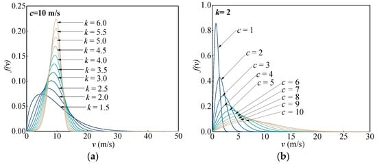
Figure 3.
Weibull distribution under different conditions: (a) c = 10 m/s; (b) k = 2.
2.2.1. Parameter Estimation Method
The values of the shape parameter k and the scale parameter c can be estimated through several methods, such as the least-square method [30], the maximum likelihood method [31], the method of moments, the method of the energy pattern factor, and the empirical method [32]. The optimal methods for different samples might differ. For example, Tian [33] compared the performance of six numerical methods and reported that the maximum likelihood method was the best method. Bilir [34] calculated the root mean square error (RMSE) values for five different methods and concluded that the empirical method performed the best. However, all methods have been reported to be applicable for most cases. The graphical method and gradient descent method were selected for the current study. The application of the graphical method requires a double logarithmic transformation of the cumulative distribution function of the wind speed. It has the advantages of simple operation with credible fitting accuracy. The equation obtained via logarithmic transformation was then solved via the gradient descent method, which improved the calculation accuracy to some extent.
Equation (2) was converted into linear form as Equation (3) [35] after double logarithmic transformation:
The observed wind speed data are classed into several intervals as 0~v1, v1~v2, …, vn−1~vn, and the frequency of each interval is f(v1), f(v2), …, f(vn). The cumulative frequency is then F(v1), F(v2), …, F(vn). By assuming this, the following equations can be obtained [35]:
For Y = y1, y2, …, yi, X = x1, x2, …, xi, Equation (3) can be described as Y = aX + b, where
The solution to determine parameters a and b here was the gradient descent method. The traditional least square method obtains the analytic solution via derivation from the loss function, whereas the gradient descent method transfers error through derivation and approaches the final solution step-by-step in an iterative way. The quadratic loss function [36] is adopted during computation:
where am and bm are the parameters participating in the mth iteration, and the initial values of a0 and b0 should be set before computing. The parameters can be obtained according to Equations (9) and (10) [36]:
where r is the learning rate and Am−1 and Bm−1 are the descent gradients of parameters a and b in the mth iteration, which are obtained by taking the partial derivative of the loss function [36]:
Equations (8)~(11) are repeated until the minimum L(a,b) is obtained and the optimum values of a and b are obtained.
2.2.2. Mean Wind-Power Density
Because the instantaneous wind speed is random and fickle, the mean wind-power density calculated on the basis of the mean wind speed during a period is more suitable for assessing the wind energy at a certain location. Once the shape parameter k and scale parameter c are determined, the mean wind-power density of the location can be described by Equation (13) [37]:
2.3. Random Forest Model
Compared with other machine learning algorithms, random forests (RFs) are widely used because of their greater robustness against multicollinearity and nonnormal distributions of the input variables [38]. RFs also have a high tolerance for outliers and effectively control overfitting. The RF algorithm has been applied to water environment research, such as water demand and rainfall forecasts [39,40]. Therefore, the RF algorithm was selected for the current study. Considering that the input and output series of the prediction model are continuous values, the regression random forest algorithm was adopted, and the steps of this algorithm are as follows [41]:
First, subtraining sets of each decision tree were extracted from the whole training set via the bootstrap method, and the unsampled data formed an out-of-bag (OOB) set. The size of each subset was the same as that of the original training set.
Next, for each tree, several characteristic variables were randomly selected from all the variables, and the best variables and split points were determined from the selected characteristic variables.
The tree subsequently grew continuously through the above step until the minimum size of the leaf node size was reached.
Finally, the decision trees were combined into a random forest, and the average value of the predicted results for all trees was considered to be the result.
The RF model was built on the basis of the random regressor function, which is used in the ensemble package of the sklearn module in Python.
3. Results and Discussion
3.1. The Correlation Between Wind Field and Turbidity
According to existing studies, wind-induced waves in shallow water bodies are the dominant factor for sediment suspension, and the turbidity values are supposed to increase accordingly. However, factors such as wind speed, wind direction and temperature are interrelated and jointly affect the change in turbidity. The response of turbidity to the wind field is nonlinear and complex.
- (1)
- The gray areas in Figure 4 were typically characterized by the significant increases in turbidity due to strong winds. These mainly appeared from January to April and October to December, that is, in early spring, winter and late autumn. The prevailing winds during these periods were northwest winds, and strong enough to cause sediment suspension. Because the water intake is limited to the southeast shore, the flow formed by the northwest wind will also carry the suspended solid from other areas to the observation site.
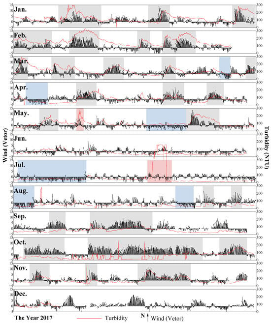 Figure 4. The time series of synchronized turbidity and wind field in the year 2020.
 - (2)
- The blue areas indicated that the wind was relatively strong but the turbidity fluctuated slightly, and appeared mainly in late spring and summer dominated by the south-easterly winds. During these periods, the wind speed was weaker than that in winter, while the wind direction was chaotic.
- (3)
- Conditions with weak wind energy with large increases in turbidity also appeared occasionally, that is, the red areas. Chemical and biological factors should be considered during these periods.
- (4)
- In other conditions, the series of turbidity and wind field were relatively weak and stable. And the turbidity of these periods came mainly from background values caused by factors like the light intensity and particle size.
Thus, detailed analysis of seasonal characteristics of the wind conditions and the responding turbidity was observed afterwards.
3.2. Seasonal Characteristics of the Wind Conditions in the Water Intake Area
3.2.1. Description of the Wind Data
There were 34,510 wind samples collected in this study, with 1.58% missing data, accounting for 2.25%, 2.45%, 0.11%, and 1.49% of the data from 2017 to 2020, respectively. And the missing data were supplemented by linear interpolation. The samples were classified into 16 wind directions and 13 wind speed intervals to better describe the wind distribution of each year and each season (spring ranged from March to May; summer ranged from June to August; autumn ranged from September, October, and November; and winter ranged from December to February).
The mean wind speed and wind direction distributions for each year and season were determined and are shown in Figure 5. Table 1 also shows the dominant wind direction results. According to the statistical results from the measured data, the WS in the water intake area was relatively low, with an annual average value of 3.3 m/s and a median speed of approximately 3 m/s. In other words, the wind speed was less than 3 m/s in more than half of the cases and less than 8 m/s in nearly 95% of the samples. The distribution frequency of each wind direction was almost equivalent, although the frequency of southwesterly winds (SSW, SW, WSW) was only 7.2%, with the smallest speed of approximately 2 m/s on average. Southeasterly winds (ESE, SE, SSE) had the highest frequency of 29.3%, but the wind speed was relatively low, with a yearly mean value of 1.8~3.1 m/s, and not greater than 5 m/s most of the time. Northwesterly winds (NNW, NW, WNW) with a frequency of 20.9% had the greatest mean speed of 4.6~5.4 m/s during the analysis period. Northeasterly winds (NNE, NE, and ENE) represented 20.0% of all samples and presented an annual average speed of 3.2~4.4 m/s.
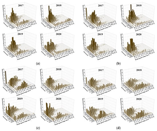
Figure 5.
Wind frequency distribution of: (a) spring; (b) summer; (c) fall; (d) winter.

Table 1.
Seasonal dominant wind direction in 2017~2020.
Because the Taihu Basin is located in the midlatitude region and belongs to the northern subtropical climate zone, it is characterized by an obvious monsoon climate with four distinct seasons, and the seasonal difference in wind conditions here is particularly evident. The relatively similar distribution of wind conditions in 2017~2020 revealed a pattern of seasonal change at this location. The pattern is consistent with that observed by Zhao et al. [42], which illustrates that the shift law of the wind has long-term stability.
In winter, the Siberian high forms over the East Asian continent because of the low temperatures (Figure 5). The wind blowing from the continent to the sea is referred to as the East Asian winter monsoon, which is guided by northwest winds. It was obvious that northwesterly winds prevailed in this season, accounting for 40% of the time, and were associated with relatively strong wind speeds. The wind speeds were mainly located within the interval of 3~7 m/s, while the range was 1–4 m/s for the other directions, resulting in the highest average speed (up to 4 m/s) in winter compared with that in the other seasons. In addition, severe winds with speeds exceeding 10 m/s were relatively common. Notably, the dominance of northwesterly winds was weak in 2017. However, this could be explained by considering the high rate of missing data (3.01%, Table 1) in the winter of this year.
The summer monsoon is also caused by the temperature difference between the ocean and continent (Figure 5). Because lands warm faster than oceans do, high pressure forms over the continent, low pressure occurs over the oceans in summer, and air then blows from the southeastern seas to the East Asian continent. This causes southeasterly winds to be dominant in this season, with a distribution frequency of 40~50%. Because of the smaller temperature difference in summer than in winter, the corresponding wind speeds are weaker. Most southeasterly winds were within the interval of 1~4 m/s on the basis of our data, which resulted in the lowest mean wind speed among the four seasons, which was less than 3 m/s (Table 1). Although a relatively similar distribution was observed in summer, wind speeds higher than 8 m/s were more common in 2018 than in the other years, and the mean wind speed in summer was the highest. According to the annual report of the water regime in the Taihu Basin and southeastern rivers [43], several typhoons, such as typhoons “Maria” and “Anbi”, made landfall in this area in the summer of 2018. Moreover, the greater intensity of these storms compared with those in former years, as well as the timing and affected region, contributed to the occurrence of extreme winds.
Spring and fall are transitions between monsoon seasons, and the winds are characterized by changing directions (Figure 5). From early spring to late spring, the winter monsoon gradually decreases, and the summer monsoon gradually increases as the wind speed decreases. The prevailing southeasterly winds accounted for approximately 30~40% of the time in spring according to the observed data (Table 1). The proportion was smaller than that in summer but larger than that in winter. On the other hand, northwesterly winds accounted for 15~20% of all data in spring, which was a higher percentage than that in summer but lower than that in winter. The mean wind speed in spring was between that in summer and that in winter, with a value of 3~3.7 m/s.
In contrast to the winds in spring, the winter monsoon increases, and the summer monsoon gradually decreases from early fall to later. Compared with the other three seasons, a relatively even wind direction distribution was identified in fall. There were multiple dominant directions in fall during the study period (Table 1), and the NNE, NNW, and NW winds represented the dominant mode. Northwesterly and southeasterly winds accounted for approximately 23–27% and 17–20% of the period, respectively, with values between those of summer and winter. As in spring, the average wind speed in fall generally hovered between the values for summer and winter (Table 1). Notably, deviations may have appeared when the percentage of missing data exceeded 3%. Specifically, the mean wind speed in fall was greater than that in winter in 2017, but on the basis of the theoretical analysis, it should have been lower. Similarly, in 2018, the mean WS in fall was lower than that in summer, which contrasted with normal conditions.
3.2.2. Seasonal Weibull Distribution of the Wind Conditions
Both the shape parameter k and the scale parameter c play roles in determining the curve of the actual shape of the Weibull distribution. The samples were divided into 256 sets of subsamples according to year, season and wind direction, and the parameters of each set were subsequently calculated. The fitting result for spring 2017 was taken as an example and is shown in Figure 6 (the results of other periods have been omitted because they show similar results). The fitting curve matched the actual distribution well, especially for southeasterly and southwesterly winds, which exhibited a unimodal distribution. Deviations arose from cases with multipeak distributions, mainly because the two-parameter Weibull model is a positive skewed distribution function with one peak.
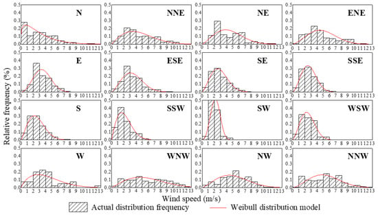
Figure 6.
Fitting of the Weibull function in spring 2017.
To further inspect the fitting accuracy quantitatively, the Spearman correlation coefficient and mean relative error (MRE) were adopted [36].
where is the frequency in interval vi−1~vi according to the Weibull distribution function; is the grade of and is the grade of ; and are the average grades; n is the amount of the intervals.
The fitted results are presented in Figure 7. The mean relative error ranged from 14.60 to 39.85% and was less than 30% in most cases. This result was reasonable considering that the frequency in some wind speed intervals was relatively small, which may have caused a high MRE. The correlation coefficient demonstrated a range of 0.84~0.96 and was above 0.9 for most periods (p < 0.01). In general, a coefficient smaller than 0.4 indicates a weak correlation, a moderate correlation arises for values between 0.4 and 0.8, and a strong correlation is defined when the coefficient exceeds 0.8. Further, the Weibull function appeared to be prominent among the commonly used distribution models for the current samples; thus, it was applicable to describe the distribution pattern in this study (Figure 8).
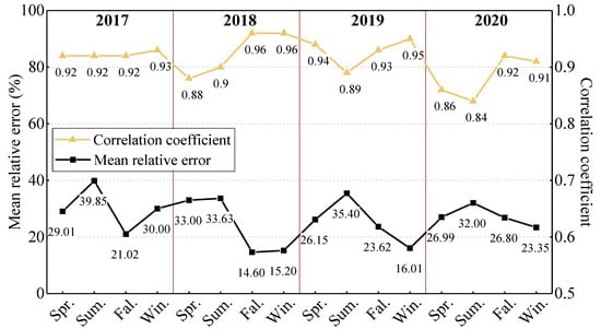
Figure 7.
Accuracy of the Weibull distribution model of the wind field.
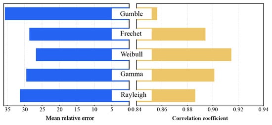
Figure 8.
The comparison of different distribution models.
The calculated parameters k (Figure 9) and c (Figure 10) of each year and season are described in a rose diagram. From Figure 9, it can be observed that the values of the shape parameter k in spring and fall (with average values of 1.91 and 1.83, respectively) were slightly higher than those in summer and winter (with average values of 1.72 and 1.73, respectively), and a larger k value indicates that the wind speed is concentrated near the central wind speed (i.e., the wind speed with a peak probability) according to the analysis in Section 3.3. Distinct laws for different wind directions or yearly scales were not found here. For the scale parameter c, it was obvious that northwesterly winds resulted in larger values of the parameter than the other directions. Considering that a greater c value represents a greater central wind speed, the conclusion that northwesterly winds showed stronger correlation with c values of 4–8 contrasts with the lower c values obtained for southwesterly winds of 1–3. This consistency confirms the effectiveness of the Weibull distribution function used in this study. Moreover, the c parameter in fall had a relatively low value overall, revealing weak wind speeds during this season.

Figure 9.
Values of parameter k for the distributions of the wind pattern.

Figure 10.
Values of parameter c (m/s) for the distributions of the wind pattern.
3.2.3. Wind-Power Density of the Water Intake Area
The mean wind-power density (Equation (13)) of each direction was subsequently obtained on the basis of the shape and scale parameters, as shown in Figure 11. Distinct differences in the power density among the 16 directions were observed in that the winds of the ESE, SE, SSE, S, SSW, SW, and WSW winds carried relatively low energies of less than 50 W/m2 due to their low speeds. Northwesterly winds (WNW, NW, and NNW) featured the greatest power density of 100~300 W/m2, and the power density even reached 500 W/m2 in 2018. With respect to the seasonal discrepancy, there was no evident difference among the four seasons in terms of the power density of each wind direction. The reason was that the power density was determined by the two Weibull parameters, that is, the distribution pattern, which showed apparent differences among directions rather than seasons. Notably, the power density in 2018 was higher than that in the other years, which was also consistent with the fact that greater wind speeds were observed because of the frequent and intensive typhoons in that year.
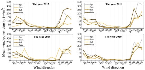
Figure 11.
The mean wind-power density of each wind direction.
3.3. Seasonal Characteristics of Turbidity in the Water Intake Area
3.3.1. Description of Turbidity
There were 32,488 turbidite samples collected in this study, with 7.35% missing data, accounting for 12.88%, 0.27%, 14.88%, and 0.47% of the data from 2017 to 2020, respectively. The distribution of the turbidity data is presented in Figure 12 according to year and season. In general, a left-skewed distribution and Gaussian fit line are observed under all conditions. Almost half of the samples were in the range of 0~60 NTU, and cases with turbidity values higher than 140 NTU accounted for less than 15% of the data. According to the results of existing studies, the greater the wind speed is, the higher the concentration of suspended sediment in water, thus increasing turbidity. Therefore, a seasonal variation in turbidity should be observed because of the seasonal distribution of the wind field at this location.
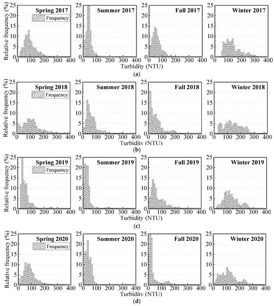
Figure 12.
Frequency distribution of turbidity data across the years: (a) 2017, (b) 2018, (c) 2019, and (d) 2020.
As shown in Figure 12 (the red line is the Gaussian fit of the frequency distribution), discrepancies in the turbidity distributions among the four seasons were indeed found, and each year exhibited a similar pattern during the study period. The turbidity in winter clearly reached the highest level, which corresponded to the greatest wind speeds. The peak of the curves, that is, the mean turbidity, ranged from 120 to 140 NTU. The smallest peak frequency and flattest curve indicate that the turbidity distribution in winter was scattered, with frequent extreme cases. The interval of 50~130 NTU represented nearly 50% of all the samples in winter, whereas the cases with turbidity greater than 200 NTU accounted for only approximately 15%. Considering that the wind speeds were lowest in summer, the turbidity level was correspondingly the lowest in this period, and the fitting distribution curves of this season obtained the highest peak frequency values and narrowest distribution ranges. The mean value was only in the range of 35~50 NTU, with more than half of the cases located in a narrow interval of 30~60 NTU. The turbidity levels in spring and fall were between those in winter and summer, with mean values of 60~90 NTU and 55~75 NTU, respectively, which was consistent with the seasonal variation in the wind speed. According to the analysis conducted in Section 3.2.1, the wind speeds in 2018 reached relatively high levels compared with those in the other years during the study period, thus causing the highest turbidity level in 2018. As shown in Figure 12b, the peak of the fitting curves shifted rightwards in 2018 compared with the same season in the other years, indicating a higher mean level of turbidity. The relatively flat curves indicate a larger span of the frequency distribution and a greater degree of data dispersion than those in 2017, 2019 and 2020. All these statistical indicators helped to confirm the increase in turbidity, as well as the greater intensity of turbidity fluctuations in 2018.
3.3.2. Seasonal Weibull Distribution of Turbidity
The Weibull function was also used to determine the distribution pattern of turbidity. The Spearman correlation coefficient and mean relative error (MRE) of the actual frequency and fitted frequency are shown in Figure 13. The correlation coefficient was in the range of 0.5–0.9 and was above 0.7 for most conditions, which showed a moderate or strong correlation between the actual and fitted frequency distributions. The mean relative error ranged from 14.36 to 67.79%, while nearly half of the periods had an MRE higher than 50%. However, considering that the rank correlation was more useful in this study to find the distribution similarity between the two series, more attention should be paid to the correlation coefficient; therefore, the Weibull function seems to be applicable for describing the distribution pattern here.
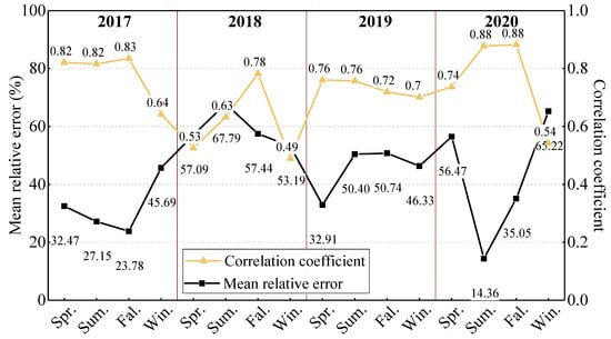
Figure 13.
Accuracy of the Weibull distribution model of turbidity.
The calculated parameters k (Figure 14) and c (Figure 15) of the turbidity of each set are shown in Figure 14 and Figure 15, respectively, according to different years and seasons. From the perspective of the season, the values of the two parameters in spring and winter obviously increased. More concentrated distribution patterns and higher central turbidity (i.e., turbidity with a peak probability) were indicated for the two seasons, whereas right-skewed distributions with lower central turbidity were obtained in fall and summer. This seasonal variation was found in all four years. From the perspective of the wind direction, the k values seemed to be greater under southerly winds than under northerly winds. However, the r c values tended to differ, being greater with northwesterly winds and lower with southeasterly winds. This means that northwesterly winds always resulted in high turbidity in the water intake area, and lower turbidity but dramatic fluctuations were obtained under the latter conditions. This was attributed to the diverse wind speeds under different conditions, and the direction of the shoreline was also influential.

Figure 14.
Values of parameter k for the distributions of the turbidity pattern.

Figure 15.
Values of parameter c (NTU) for the distributions of the turbidity pattern.
3.4. Correlation Between Wind-Power Density and Turbidity
To observe the similarity of the turbidity and wind distribution patterns, the correlation between the two Weibull distribution parameters within the same period was derived via a rose diagram. The results (Figure 16) revealed a strong correlation with the scale parameter c, with most coefficients ranging from 0.4 to 1.0, whereas a relatively weak and even negative correlation was observed for the shape parameter k, with values ranging from −0.8 to 0.4. This means that the peak values of turbidity and wind speed seemed to occur at a similar position in the distribution within the same period, but discrepancies existed in the distribution curves. Another reason for this may be the critical wind speed; once the critical value was exceeded, that is, the wind speed was high enough, the sediment of the bottom layer was stimulated immediately and caused high turbidity. However, under weak wind speeds, other factors, such as the wind direction distribution and duration, played relatively more important roles in turbidity variations. The threshold value was approximately 3 m/s for onshore winds and 4 m/s for offshore winds from our previous study [3].
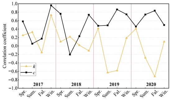
Figure 16.
Correlations between the corresponding Weibull parameters.
Many studies conducted in typical shallow lakes have confirmed the strong correlation between wind conditions and suspended sediment in water bodies. As the wind blows over the water surface, the wind energy is transferred from the surface to the bottom layer and then waves. The wave-induced shear stress is the dominant factor [44] contributing to sediment suspension and migration, thus resulting in variations in the suspended sediment concentration and later turbidity in the local area. The wind-power density of each direction was combined with the distribution frequency to describe the weighted power density () via Equation (16).
where is the wind-power density of the wind direction j and where is the distribution frequency of the wind direction j.
The weighted wind power density and seasonally averaged turbidity results are shown in Figure 17, and the seasonal mean wind speed is also given for comparison. Furthermore, the weighted superimposed value of the wind (WSV) proposed in previous work [3] was also determined, which takes into account the dominant wind direction, as well as the delay effect of wind on turbidity. In general, the change in turbidity was closely related to the weighted wind-power density, with a correlation coefficient of 0.83 (r2 = 0.7), which was significantly greater than the WSV (r2 = 0.58), indicating a strong statistical correlation. The correlation between turbidity and wind speed was relatively weak, with a coefficient of 0.64 (r2 = 0.41). A distinct increase in turbidity was obtained when the distribution of the wind conditions during the period was comprehensively considered rather than the wind speed alone.
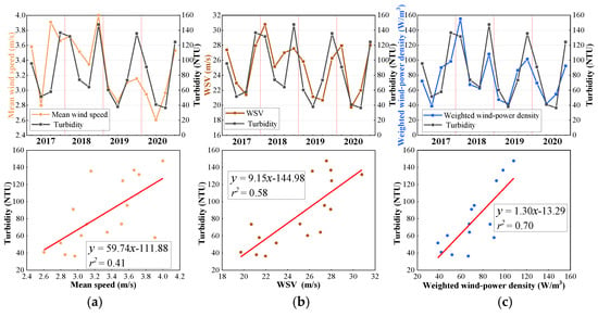
Figure 17.
Comparison of turbidity series to (a) mean wind speed; (b) WSV; (c) weighted wind-power density.
However, obvious deviations appeared in the winter of 2017, and the mean turbidity was relatively high but with a correspondingly low wind-power density. Moreover, this circumstance was also observed in the other winters during the study period but with a lower intensity. This might be attributed to neglecting the duration of the wind, as well as the influence of the shoreline near the water intake area. Being controlled by northerly winds (including northeasterly and northwesterly winds) was the most important feature for winter. Because the shoreline near the water intake extends in a southwest direction, the flow field formed by the durative action of northwesterly winds facilitates sediment accumulation at the study location. Specifically, the southeastward flow carries suspended sediment from other areas of the lake to the water intake area in this situation, and the resistance of the lake shore impedes the diffusion of suspended matter to some extent. In addition, long winds and persistent, strong northwesterly winds also cause sediment suspension to occur more easily in these locations [3]. All these factors drive the concentration of suspended sediment to increase more effectively compared to the other seasons. However, the response of turbidity to wind might be complex, and a deeper mechanism could not be investigated in this study, resulting in minor deviations.
3.5. The Prediction Model of Turbidity Based on the Wind Field Distribution
A previous study proposed a random forest prediction model of turbidity based on the weighted superposed value of the wind (WSV) and air temperature. Compared with the original input variables, the correlation between the predicted turbidity series and the actual series reached 0.8, and the MRE was less than 30% when the database was constantly updated. However, the model runs on hourly data, which means that the predictive step length is not long enough for adjusting the dosage of water. Furthermore, the WSV was only a simple superposition of the wind speed and direction but failed to consider the distributions of the wind speed and direction. A turbidity prediction model promoted by weighted wind-power density is subsequently presented in this study.
3.5.1. Model Building
- Screening of input variables
Turbidity is subject to not only the wind conditions, but also the biochemical factors, which are closely related to temperature. Temperature affects turbidity by influencing the physicochemical processes of organic matter, such as the reaction rate of various enzymes in algae, the utilization efficiency of nutrients in water and the metabolic rate of algae. However, the specific mechanism is quite difficult to accurately quantify. Therefore, we selected air temperature as a comprehensive index to quantify various biochemical factors affecting turbidity.
As shown in Figure 18, the seasonal fluctuation cycle of temperature and turbidity was extremely similar with a negative correlation. However, the linear mapping relationship between the two series is not clear. Therefore, the seasonal cycle sequence of air temperature was adopted as one input in the current model. It was extracted by decomposing the original sequence through EMD to maximize the retention of temperature trends and filter outliers, which obviously improved the model performance.
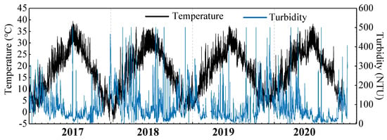
Figure 18.
Comparison of turbidity and temperature series.
Furthermore, to observe the enhancing effect of the wind power density on model accuracy, three combinations of input variables were fed to the model, as shown in Table 2.

Table 2.
Combinations of input variables.
- 2.
- Data preprocessing
The turbidity data collected by the online turbidimeter were affected by interference factors, such as bubble pollution and illumination intensity. Therefore, the method of quartile rejection based on the moving window was adopted to eliminate outliers and improve the model performance. By sharing the samples, the effects of the segmentation boundary could be reduced, and more anomalies could be found. The window length was set to 360, and the upper and lower limits of rejection were calculated via Equations (17)–(19) [8]:
where Q0.75 and Q0.25 are the upper and lower quartiles of the samples, respectively, and h is the interquartile range, which indicates the dispersion degree of the middle 50% of the data.
Lu = Q0.75 + 2.5 h
Ld = Q0.25 − 2.5 h
h = Q0.75 − Q0.25
According to the seasonal characteristics of the correlation between the wind field and turbidity, the time span was assumed to be a quarter. However, the turbidity of the water was monitored daily, and the dosage was adjusted every month. Thus, the time span of the mean wind speed, WSV, and weighted wind-power density was taken as one month.
According to the seasonal characteristics of the correlation between the wind conditions and turbidity, the time span was assumed to be a quarter. However, the turbidity of the water was monitored daily, and the dosage was adjusted every month. Thus, the time span of the mean wind speed, WSV, and weighted wind-power density was taken as one month.
- 3.
- Parameter setting for the random forest algorithm
The most influential parameters for the performance of the random forest model are n_estimators, max_depth, and max_features. n_estimators refers to the number of decision trees. More trees denote higher accuracy but increase the calculation time. max_depth represents the maximum splitting depth of trees. A large value of the parameter implies a better fitting effect but an increasing risk of overfitting. max_features contributes to the maximum number of features to be considered in split nodes, which is related to the model performance but at the cost of the growth time of the trees. Therefore, the optimal combination of parameters should be found through a trial-and-error method for the test set of each model. The OOB data generated by bootstrapping could be used to verify the accuracy of the model without cross-validation, thereby improving the validation efficiency. The optimal parameter combination was determined on the basis of the accuracy of the OOB data (OOB_score parameter). The final results are shown in Table 3.

Table 3.
Summary of the model parameters.
3.5.2. Modeling Results
The sample size was 25,312, and the missing values and abnormal values accounted for 7.56% and 3.93%, respectively. All of these samples were omitted from the modeling. Each model was run five times, and the average of the predicted values and the MRE were used as the analysis objects. The MREs of models ①, ②, and ③ were 66.4%, 38.8% and 29.4%, respectively. A further comparison of the prediction results and the actual values is shown in Figure 18. In general, the results indicate that the application of weighted wind-power density improved the model performance to some extent.
From the line chart in Figure 19, the predicted values and the actual values showed similar trends, especially for the model fed with weighted wind-power density. Model ① performed better in the period in which turbidity transformed steadily, whereas for Model ②, higher accuracy occurred at peak points of turbidity instead. Model ③ achieved stable performance for both the peak values and other samples.
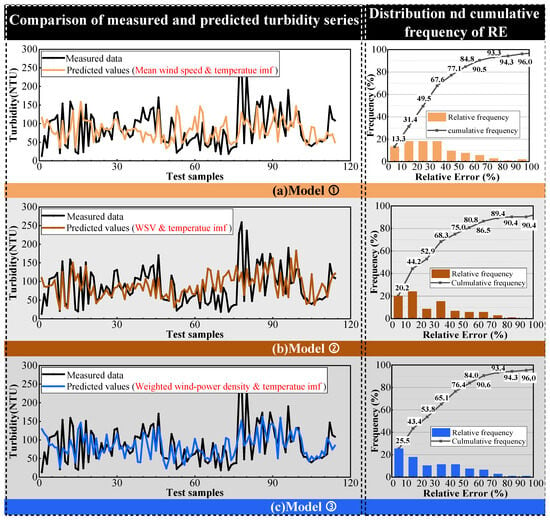
Figure 19.
Modeling results of (a) Model ①; (b) Model ②; (c) Model ③.
The frequency statistics also demonstrated the same result. For the model that used the mean wind speed only, the proportion of predicted values within 10% RE was only 13.3%, whereas it was 20.2% for the model with the WSV as input. When the weighted wind-power density was used, the proportion increased significantly to 25.5%. Nearly half of the test samples of Models ② and ③ had RE values less than 20%, which was enough for the waterworks to adjust the dosage in advance. Furthermore, 90% of the test samples received an RE of less than 70%, which can provide an important reference for adjusting water.
With a simple input of only wind and temperature data, the present model was not inferior to the reported models based on multiple inputs. The data were treated at the one-month scale; therefore, the model could make a satisfactory prediction of turbidity for at least one month in advance.
4. Conclusions
The current study investigated the seasonal law of wind conditions and turbidity fluctuations in Taihu Lake through waterworks with the lake as the water source. A relatively high correlation of the two factors was achieved by introducing the Weibull distribution function and the mean wind-power density. The results provide ideas for studying the influence mechanism of the effect of wind on turbidity changes. Compared with previous methods, the turbidity prediction model built on the basis of the mean wind power density achieved better accuracy with fewer input variables. This allows for time to adjust the water treatment process, which further contributes to emergency management. The main conclusions that can be drawn are as follows:
- The seasonal differences in the wind conditions at the observed locations were particularly distinct. Northwesterly winds prevailed over the lake surface with the greatest wind force in winter, whereas southeast winds dominated in summer with the lowest speed among the four seasons. In addition, spring and fall are transitions between monsoon seasons, which are characterized by changing wind directions with multiple dominant directions. Compared with the seasonal variation in turbidity of the area, it can be concluded that northwest winds were more likely to cause turbidity to increase.
- With the Weibull distribution, northwest winds were verified to be the greatest wind force compared with other directions. The actual distribution and the fitted Weibull curve were strongly correlated, confirming the effectiveness of the function for the current study. The peak values of the two parameters appeared at similar positions for the wind conditions and turbidity within the same period, whereas the distribution curves were relatively different, which may be caused by a critical wind speed.
- The weighted wind-power density was proposed by taking into account the wind distribution in a period rather than the wind speed alone, leading to a strong correlation of the item with the seasonally averaged turbidity.
- The turbidity prediction model built with the mean wind-power density and temperature component extracted via EMD as input achieved good performance in both periods in which the turbidity transformed steadily and fluctuated greatly. Compared with previous methods, the results of the model promoted both forecast accuracy and feasibility in terms of the application and pretreatment of the wind data.
5. Suggestions
The results of the present study can serve as a reference for other waterworks with shallow lakes as sources. However, more studies must be carried out to improve model performance, as well as to control turbidity.
- In this study, we innovatively applied the Weibull distribution model to turbidity series to observe the similarity of the time distribution of the two variables. However, the accuracy of the distribution model was supposed to be optimized further by improving the model parameters, which would also be helpful for the performance of the prediction model.
- The proposed model achieved turbidity prediction one month in advance, with an RE less than 30%. By optimizing the input variables, further efforts are needed to find a more appropriate scale that can meet the needs of the emergency treatment of water and achieve relatively high accuracy.
- This work explored the relationship between turbidity and the wind field but failed to discover further reasons for this phenomenon, such as the hydraulic characteristics and sediment distribution under the wind effect in shallow lakes. Therefore, further work should focus on this problem according to hydraulics and sediment dynamics theory.
- Attention should also be given to turbidity reduction measurements on the basis of current and further work, such as dosage adjustments, the application of breakwaters and even the development of water quality management platforms combined with prediction models.
Author Contributions
Conceptualization, Supervision, Y.Z.; Methodology, Validation, Formal Analysis, Data Curation, Writing—original draft, Writing—Review and Editing, Visualization, X.Y. All authors have read and agreed to the published version of the manuscript.
Funding
This research received no external funding.
Institutional Review Board Statement
Not applicable.
Informed Consent Statement
Written informed consent has been obtained from the patient(s) to publish this paper.
Data Availability Statement
The original contributions presented in this study are included in the article. Further inquiries can be directed to the corresponding author.
Conflicts of Interest
The authors declare that they have no competing interests.
Abbreviations
| EMD | Empirical mode decomposition |
| RE | Relative error |
| RF | Random forests |
| OOB | Out-of-bag |
| MRE | Mean relative error |
| R | Spearman correlation coefficient |
| WSV | The weighted superposed value of the wind field |
References
- Yue, S. Turbidity of water. China Water Wastewater 1995, 11, 33–35. (In Chinese) [Google Scholar]
- Wu, T.F.; Qin, B.Q.; Zhu, G.W.; Zhu, M.Y.; Wei, L.I.; Luan, C.M. Modeling of turbidity dynamics caused by wind-induced waves and current in the Taihu Lake. Int. J. Sediment Res. 2013, 28, 139–148. [Google Scholar] [CrossRef]
- Yao, X.; Liu, X.; Zhou, Y.; Zhang, L.; Zhou, Z.; Zhang, Y. The influence of wind-induced sediment resuspension and migration on raw water turbidity in Lake Taihu, China. Environ. Sci. Pollut. Res. 2022, 29, 84487–84503. [Google Scholar] [CrossRef]
- Bohling, B. Measurements of threshold values for incipient motion of sediment particles with two different erosion devices. J. Mar. Syst. 2009, 75, 330–335. [Google Scholar] [CrossRef]
- Tang, C.; Li, Y.; He, C.; Acharya, K. Dynamic behavior of sediment resuspension and nutrients release in the shallow and wind-exposed Meiliang Bay of Lake Taihu. Sci. Total Environ. 2020, 708, 135131. [Google Scholar] [CrossRef] [PubMed]
- Jin, K.; Ji, Z. Calibration and verification of a spectral wind-wave model for Lake Okeechobee. Ocean Eng. 2001, 28, 571–584. [Google Scholar] [CrossRef]
- Zhang, P.; Chen, X.; Lu, J.; Zhang, W. Assimilation of remote sensing observations into a sediment transport model of China’s largest freshwater lake: Spatial and temporal effects. Environ. Sci. Pollut. Res. 2015, 22, 18779–18792. [Google Scholar] [CrossRef]
- Zhao, J.X.; Ding, W.H.; Xu, S.K.; Ruan, S.P.; Wang, Y.; Zhu, S.L. Prediction of sediment resuspension in Lake Taihu using support vector regression considering the cumulative effect of wind speed. Water Sci. Eng. 2021, 14, 228–236. [Google Scholar] [CrossRef]
- Luo, L.; Qin, B.; Hu, W.; Ji, J.; Zhang, B. Wave characteristics in Lake Taihu. J. Hydrol. 2004, 19, 662–670. (In Chinese) [Google Scholar]
- Hu, K.M.; Pang, Y.; Yu, H.; Wang, H. Simulation study on water quality based on sediment resuspended experiment in Lake Taihu. Resour. Environ. Yangtze Basin 2011, 20 (Suppl. 1), 94–99. (In Chinese) [Google Scholar]
- Cao, Z.; Kong, L.; Jiao, G. Initiation of sediment movement for a wave-current coexistent system. Acta Oceanol. Sin. 2003, 25, 113–119. (In Chinese) [Google Scholar]
- Zhou, Y.R.; Yin, C.A. Criterion for the initiation of sediment movement in different boundary layers under oscillatory waves. Int. J. Sediment Res. 2004, 1, 8. (In Chinese) [Google Scholar]
- Ding, W.; Zhao, J.; Qin, B.; Wu, T.; Zhu, S.; Li, Y.; Xu, S.; Ruan, S.; Wang, Y. Exploring and quantifying the relationship between instantaneous wind speed and turbidity in a large shallow lake: Case study of Lake Taihu in China. Environ. Sci. Pollut. Res. 2021, 28, 16616–16632. [Google Scholar] [CrossRef] [PubMed]
- Lou, S.; Huang, W.; Liu, S.; Zhong, G.; Johnson, E. Hurricane impacts on turbidity and sediment in the Rookery Bay National Estuarine Research Reserve, Florida, USA. Int. J. Sediment Res. 2016, 31, 330–340. [Google Scholar] [CrossRef]
- Iglesias, C.; Martínez Torres, J.; García Nieto, P.J.; Alonso Fernández, J.R.; Díaz Muñiz, C.; Piñeiro, J.I.; Taboada, J. Turbidity Prediction in a River Basin by Using Artificial Neural Networks: A Case Study in Northern Spain. Water Resour. Manag. 2014, 28, 319–331. [Google Scholar] [CrossRef]
- Yang, T.M.; Fan, S.K.; Fan, C.; Hsu, N.S. Establishment of turbidity forecasting model and early-warning system for source water turbidity management using back-propagation artificial neural network algorithm and probability analysis. Environ. Monit. Assess. 2014, 186, 4925–4934. [Google Scholar] [CrossRef]
- Abba, S.I.; Abdulkadir, R.A.; Gaya, M.S.; Saleh, M.A.; Esmaili, P.; Jibril, M.B. Neuro-fuzzy ensemble techniques for the prediction of turbidity in water treatment plant. In Proceedings of the 2019 2nd International Conference of the IEEE Nigeria Computer Chapter (Nigeria Computer Conference), Zaria, Nigeria, 14–17 October 2019; IEEE: Piscataway, NJ, USA, 2019. [Google Scholar]
- Zounemat-Kermani, M.; Alizamir, M.; Fadaee, M.; Sankaran Namboothiri, A.; Shiri, J. Online sequential extreme learning machine in river water quality (turbidity) prediction: A comparative study on different data mining approaches. Water Environ. J. 2020, 35, 335–348. [Google Scholar] [CrossRef]
- Wang, J.; Yuan, Y.; Yu, Z.G.; Qu, S.; Li, W. Effect of turbulence driven by wind on sediment suspension under different submerged vegetation density in Lake Taihu. Ecol. Indic. 2023, 154, 110767. [Google Scholar] [CrossRef]
- Shi, W.; Zhu, L.; Van Dam, B.; Smyth, A.R.; Deng, J.; Zhou, J.; Pan, G.; Yi, Q.; Yu, J.; Qin, B. Wind induced algal migration manipulates sediment denitrification N-loss patterns in shallow Taihu Lake, China. Water Res. 2022, 209, 117887. [Google Scholar] [CrossRef]
- Dargahi-Noubary, G.R. New Method for Prediction of Extreme Wind Speeds. J. Eng. Mech. 1989, 115, 859–866. [Google Scholar] [CrossRef]
- Akgül, F.G.; Şenoğlu, B.; Arslan, T. An alternative distribution to Weibull for modeling the wind speed data: Inverse Weibull distribution. Energy Convers. Manag. 2016, 114, 234–240. [Google Scholar] [CrossRef]
- Mohammadi, K.; Alavi, O.; Mostafaeipour, A.; Goudarzi, N.; Jalilvand, M. Assessing different parameters estimation methods of Weibull distribution to compute wind power density. Energy Convers. Manag. 2016, 108, 322–335. [Google Scholar] [CrossRef]
- Saleh, H.; Aly, A.A.E.A.; Abdel-Hady, S. Assessment of different methods used to estimate Weibull distribution parameters for wind speed in Zafarana wind farm, Suez Gulf, Egypt. Energy 2012, 44, 710–719. [Google Scholar] [CrossRef]
- Jabbar, R.I. Statistical Analysis of Wind Speed Data and Assessment of Wind Power Density Using Weibull Distribution Function (Case Study: Four Regions in Iraq). J. Phys. Conf. Ser. 2021, 1804, 012010. [Google Scholar] [CrossRef]
- Akdağ, S.A.; Bagiorgas, H.S.; Mihalakakou, G. Use of two-component Weibull mixtures in the analysis of wind speed in the Eastern Mediterranean. Appl. Energy 2010, 87, 2566–2573. [Google Scholar] [CrossRef]
- Akpinar, E.K.; Akpinar, S. An assessment on seasonal analysis of wind energy characteristics and wind turbine characteristics. Energy Convers. Manag. 2005, 46, 1848–1867. [Google Scholar] [CrossRef]
- Wang, B. Statistic Analysis of Mean Wind Speed Based on the Joint Probability Distribution of Wind Speed, Wind Direction and Season. J. Jiamusi Uni. Nat. Sci. Ed. 2013, 2, 211–213. [Google Scholar]
- Ozay, C.; Celiktas, M.S. Statistical analysis of wind speed using two-parameter Weibull distribution in Alaat region. Energy Convers. Manag. 2016, 121, 49–54. [Google Scholar] [CrossRef]
- Davies, I.J. Empirical correction factor for the best estimate of Weibull modulus obtained using linear least squares analysis. J. Mater. Sci. Lett. 2001, 20, 997–999. [Google Scholar] [CrossRef]
- Ahmed, A.O.; Al-Kutubi, H.S.; Ibrahim, N.A. Comparison of the Bayesian and Maximum Likelihood Estimation for Weibull distribution. J. Math. Stat. 2010, 6, 100–104. [Google Scholar] [CrossRef][Green Version]
- Li, X.; Shi, Y.; Li, H. Empirical Bayes Estimation for Parameters of Weibull Distribution Family Using NA Samples. J. Kunming Uni. Sci. Tech. 2009, 2, 116–121. [Google Scholar]
- Tian, P.C. Performance comparison of six numerical methods in estimating Weibull parameters for wind energy application. Appl. Energy 2011, 88, 272–282. [Google Scholar]
- Bilir, L.; İmir, M.; Devrim, Y.; Albostan, A. Determination of Weibull Parameters for Wind Speed Distribution at Incek Region–Ankara. In Proceedings of the 4th International Conference on Nuclear and Renewable Energy Resources (NURER’14), Antalya, Türkiye, 27–30 October 2024. [Google Scholar]
- Kaoga, D.K.; Danwe, R.; Yamigno, S.D.; Djongyang, N. Performance Analysis of Methods for Estimating Weibull Parameters for Wind Speed Distribution in the District of Maroua. J. Fundam. Appl. Sci. 2015, 6, 153–174. [Google Scholar] [CrossRef]
- Huang, W. Research on Probability Distribution of Wind Speed in Wind Farm and Its Fitting Models; Guangxi University: Guangxi, China, 2021. [Google Scholar]
- Ahmed, S.A. A Statistical Analysis of Wind Power Density Based on the Weibull and Ralyeigh models of “Penjwen Region” Sulaimani/Iraq. Jordan J. Mech. Ind. Eng. 2012, 6, 135–140. [Google Scholar]
- Wang, P.; Lu, B.; Zhang, H.W.; Zhang, W.; Sun, Y.F. Water demand prediction model based on random forests model and its application. Water Resour. Prot. 2014, 30, 34–37. [Google Scholar]
- Kim, H.-I.; Kim, B.-H. Analysis of Major Rainfall Factors Affecting Inundation Based on Observed Rainfall and Random Forest. Korean Soc. Hazard Mitig. 2020, 20, 301–310. [Google Scholar] [CrossRef]
- Jeihouni, M.; Toomanian, A.; Mansourian, A. Decision tree-based data mining and rule induction for identifying high quality groundwater zones to water supply management: A novel hybrid use of data mining and GIS. Water Resour. Manag. 2020, 34, 139–154. [Google Scholar] [CrossRef]
- Liu, Y.; Wu, H. Water bloom warning model based on Random Forest. In Proceedings of the 2nd International Conference on Intelligent Informatics and Biomedical Sciences, Okinawa, Japan, 24–26 November 2017. [Google Scholar]
- Zhao, Q.H.; Chen, S.Q.; Chen, S.Y. Turbidity in response to wind speed, wind direction and wind duration in Gonghu Bay, Lake Taihu. J. Lake Sci. 2018, 30, 1587–1598. [Google Scholar]
- Wang, R.; Lyu, Z.; Yu, C.; Liu, A.; Quan, T. Joint Analysis and Morphological Characterization of HFSWR Echo Properties during Severe Typhoon Muifa. Remote Sens. 2024, 16, 267. [Google Scholar] [CrossRef]
- Sheng, Y.; Lick, W. The transport and resuspension of sediments in a shallow lake. J. Geophys. Res. 1979, 84, 1809–1826. [Google Scholar] [CrossRef]
Disclaimer/Publisher’s Note: The statements, opinions and data contained in all publications are solely those of the individual author(s) and contributor(s) and not of MDPI and/or the editor(s). MDPI and/or the editor(s) disclaim responsibility for any injury to people or property resulting from any ideas, methods, instructions or products referred to in the content. |
© 2025 by the authors. Licensee MDPI, Basel, Switzerland. This article is an open access article distributed under the terms and conditions of the Creative Commons Attribution (CC BY) license (https://creativecommons.org/licenses/by/4.0/).