Carbon Emissions Intensity of the Transportation Sector in China: Spatiotemporal Differentiation, Trends Forecasting and Convergence Characteristics

Abstract

Effectively controlling the carbon emissions intensity of the transportation sector (TSCEI) is essential to promote the sustainable development of the transportation industry in China. This study, which builds upon trend analysis, the Dagum Gini coefficient, and spatial autocorrelation analysis to reveal the spatiotemporal differentiation of TSCEI, employs both traditional and spatial Markov chain to analyze the dynamic evolution of TSCEI and forecast its future development trend. Furthermore, econometric models are constructed to examine the convergence characteristics of TSCEI. The empirical results reveal the following key findings: (1) TSCEI in China has significantly declined, exhibiting a spatial distribution pattern of “higher in the north, lower in the south; higher in the west, lower in the east”. (2) Inter-regional differences are the main contributors to overall TSCEI disparities, with provincial TSCEI exhibiting positive spatial autocorrelation, primarily characterized by high–high and low–low agglomeration. (3) TSCEI tends to gradually shift from high- to low-intensity states over time, with an equilibrium probability of 90.98% for transferring to lower intensity state. Provincial TSCEI shows significant spatial spillover effects, influenced by neighboring provinces’ states. (4) TSCEI demonstrates convergence characteristics at national and regional levels, including $\sigma$ convergence, absolute and conditional $\beta$ convergence, with the transportation energy structure and technological progress playing a particularly prominent role in facilitating the convergence of TSCEI towards lower values. The policy implications of promoting TSCEI convergence and reducing spatial inequality are discussed.

1. Introduction

The carbon emission intensity metric gauges the efficiency of carbon emissions within economic processes and serves as a crucial indicator for evaluating the efficacy of carbon reduction policies [1,2]. CO₂ has emerged as a significant contributor to global warming [3]. In 2022, global carbon emissions from fuel combustion reached 34.12 billion tons. China, the largest emitter, contributed 10.61 billion tons, accounting for 31.11% of global emissions [4] China attaches great importance to the issue of climate change and regards actively addressing it as a major strategy for the country’s socio-economic development [5]. In 2015, China established carbon control targets under the Paris Agreement, committing to peak emissions before 2030 and reduced carbon intensity by 60–65% relative to 2015 levels by 2030 [6]. In 2020, China pledged to achieve carbon neutrality by 2060. The 2021 “Action Plan for Carbon Peaking Before 2030” aims to reduce national carbon emission intensity by 18% by 2025 (compared to 2020) and by over 65% by 2030 (compared to 2005). By 2020, a 48.4% reduction had been achieved compared to 2005. To meet the 2030 goals, an additional 32.1% reduction is needed from 2020 levels. Achieving these ambitious targets necessitates that industries across the board enhance resource efficiency and foster low-carbon development [7].

The transportation sector is a major contributor to global carbon emissions [8], playing a vital role in addressing climate change and mitigating global warming [9]. In 2022, global carbon emissions from fuel combustion in the transportation sector amounted to 7.94 billion tons, accounting for 23.28% of total global carbon emissions [4]. In China, the transportation sector is also a major source of carbon emissions, accounting for 8.34% of national emissions in 2022 [4], second only to industry and buildings [10]. Moreover, from 2000 to 2022, China’s transportation sector saw an average annual carbon emissions growth rate of 6.24%, much higher than the global rate of 1.52%. In contrast, the transportation sector in developed countries represents a substantially larger share of national carbon emissions. For instance, Canada’s transportation sector accounts for 31.33% of its total emissions, the United States for 36.88%, Japan for 19.15%, the United Kingdom for 34.63%, Italy for 33.46%, Germany for 23.03%, and France for 43.59%. Compared to these developed nations, China’s transportation sector currently contributes a relatively lower proportion of national carbon emissions, despite its rapid growth rate. This disparity underscores the significant potential for emissions reduction in China’s transportation sector, particularly as the country accelerates its transition to green transportation and decarbonization efforts. Given current trends and long-term projections, reducing carbon emissions in the transportation sector is crucial for achieving China’s “dual carbon” goals. In China’s “14th Five-Year Plan for Modern Comprehensive Transportation System” and “14th Five-Year Plan for Green Transport Development,” reducing carbon emission intensity has been established as a pivotal objective for low-carbon transport development. This goal not only represents a strategic response to climate change and sustainable development, but is also essential for fostering high-quality industry growth.

Transportation sector carbon emission intensity (TSCEI) refers to the ratio of CO₂ emissions generated by transportation activities to the economic output of the transportation sector [11]. Given that the reduction in emission intensity plays a pivotal role in mitigating overall emissions, lowering carbon intensity is crucial for achieving emission reduction targets [12]. Moreover, the convergence of carbon emissions is a key indicator of declining carbon emission intensity [13] and a necessary condition for achieving the peak in carbon emissions [14,15]. In general, when provinces with higher TSCEI exhibit a faster rate of decline compared to those with lower intensity, and eventually converge toward steady-state levels, this signals the presence of the convergence phenomenon [16]. However, the effectiveness of transportation emissions reduction varies significantly across China’s provinces, resulting in an unequal distribution of carbon emissions in scale and intensity. For instance, in 2022, Guangdong Province’s transportation carbon emissions amounted to 60.06 million tons, nearly 12.32 times higher than the emissions of Ningxia, which had the lowest emissions. Therefore, balancing the transportation development needs with emissions reduction pressures across provinces necessitates the formulation and implementation of scientifically sound and effective transportation carbon reduction policies [17]. This requires a deep understanding of the dynamic evolution trend of TSCEI and its convergence characteristics. Such an understanding not only enhances the precision and effectiveness of emissions reduction policies, but also provides robust support for the low-carbon transformation of the transportation sector in China.

The research relevant to this study focuses on three key areas. The first area quantifies the carbon emission efficiency of the transportation sector. TSCEI, from a single-factor perspective, essentially reflects the carbon emission efficiency of the transportation sector during the process of economic development, serving as a tool to evaluate the green development level and environmental performance of the sector. Meanwhile, numerous studies have adopted a multifactorial input–output approach, particularly under the data envelopment analysis (DEA) framework, to measure the total-factor carbon emission efficiency. For instance, studies by Zhao, et al. [18], Domagała and Kadłubek [19], and Liu, et al. [20] have utilized the EBM-DEA model, the SBM-DEA model, and the three-stage DEA model, respectively, to calculate the carbon emission efficiency of the transportation sector. Although the total-factor perspective offers more comprehensive results, the use of differing methodologies or an input–output indicators system on the same research subject can produce variant results, potentially complicating the analysis [21]. Nevertheless, carbon emissions intensity can offer a clearer direction for policymaking, and align with China’s carbon reduction targets during its ongoing urbanization and industrialization phases. Additionally, analytical methodologies such as the Theil index, Dagum Gini coefficient, kernel density estimation, spatial autocorrelation analysis, and the standard deviational ellipse are routinely employed to assess the spatiotemporal differentiation of carbon emission intensity across nations, regions, or industries [22,23,24,25].

The second research stream aims to identify the key determinants of carbon emission intensity. Scholars have conducted extensive and detailed studies on this topic, employing methodologies that primarily consist of decomposition analysis and econometric regression analysis. Decomposition analysis focuses on identifying the contributions of various factors. For example, Yan, et al. [26] employed multiplicative structural decomposition analysis to discover that energy intensity is the primary driver of reduced carbon emission intensity in China. De Oliveira-De Jesus [27] applied the IDA-LMDI method to decompose the factors influencing power-related carbon emission intensity in Latin America and the Caribbean. Pan, et al. [28], using the LMDI method, identified that technological progress, industrial structure, and regional scale were the main contributors to the decline in China’s carbon emission intensity. Econometric regression analysis emphasizes the exploration of the causal effects between various influencing factors and carbon emission intensity, offering a richer economic interpretation compared to decomposition analysis. Numerous econometric regression models, such as panel fixed effects regression [29], panel quantile regression [30], symbolic regression [31], geographically weighted regression [32], and spatial econometric models [33], have been applied to reveal the key drivers of carbon emission intensity. Additionally, many scholars have used econometric regression models to focus on specific factors, such as smart infrastructure [34], extreme heat [35], and digital economy [36]. In the transportation sector, many scholars have similarly employed both decomposition and econometric regression analyses to explore the factors affecting transportation carbon emissions [37,38,39].

The third area of research examines the convergence of carbon emission intensity. The concept of convergence is rooted in neoclassical growth theory, describing the tendency of economic growth levels across countries or regions to converge over time [40]. Specifically, economists investigate whether mechanisms exist that allow relatively poorer economies to converge with wealthier nations, thereby reducing the income gap [41]. In the field of environmental economics, convergence models have been applied to investigate the convergence of various indicators such as per capita carbon dioxide emissions [42], eco-efficiency [43], environmental efficiency [44], and energy efficiency [45]. The convergence of carbon emission intensity has also attracted considerable scholarly attention. Apergis et al. [46] employed the Phillips-Sul (PS) method to test for club convergence in the carbon emission intensity of Central American countries. Yu et al. [15] examined the presence of $\sigma$ convergence, $\beta$ convergence, and club convergence in 24 industrial sectors across China. Zhang et al. [47] investigated the $\sigma$ convergence and $\beta$ convergence in carbon emission intensity for urban agglomerations in the Yellow River Basin. Li et al. [48] and Huang et al. [16] applied spatial convergence models to identify absolute and conditional $\beta$ convergence in the carbon emission intensity of Chinese provinces. Furthermore, Zheng and Yuan [13] found evidence of $\beta$ convergence and club convergence in sectors such as agriculture, industry, construction, transportation, wholesale, and other services in China.

The scholarly literature on the spatiotemporal distribution, determinants, and convergence tests of carbon emission intensity is extensive; however, there remain notable deficiencies that warrant further investigation. First, existing studies primarily focus on qualitative descriptions based on measures of TSCEI, or utilize statistical tools such as the Gini coefficient and Theil index to quantify spatial differences [17]. However, in-depth explorations of the spatiotemporal differentiation characteristics of TSCEI are lacking. Second, although the existing literature employs frameworks such as the LEAP model, STIRPAT models, heuristic algorithms, and machine learning techniques to forecast transportation carbon emissions [49,50,51], we are unaware of any studies that have predicted the future evolutionary trend of TSCEI in China. Third, while numerous studies have examined the convergence characteristics of core indicators of environmental economics and carbon emission intensity at the national, regional, and industry levels, few studies specifically examine the convergence of TSCEI.

Consequently, to address critical gaps in the existing research, the research motivation is articulated across three main dimensions. First, the analysis focuses on the spatiotemporal differentiation of TSCEI. This analysis not only facilitates a macroscopic understanding of the current state and fundamental characteristics of the TSCEI, but also aids in comprehensively grasping its distribution pattern, thus informing the formulation of differentiated low-carbon transportation development policies that support synergistic and sustainable growth. Second, this study forecasts the future evolution trends of TSCEI, which is crucial for facilitating decoupling between economic growth and transportation carbon emissions. This forecast is not only essential for delineating stage-specific carbon reduction targets, but also for quantitatively assessing the feasibility and challenges associated with achieving future reductions in transportation carbon emissions. Third, this study examines the convergence characteristics of TSCEI. This examination aids in assessing the viability of achieving the carbon peak target and, most crucially, in identifying the key factors promoting TSCEI convergence. This has significant scientific implications for evaluating current policy effectiveness, and for optimizing and adjusting the implementation pathways.

The marginal contributions of this study are primarily reflected in the following aspects: (1) This study goes beyond traditional spatiotemporal analysis methods by integrating trend analysis, the Dagum Gini coefficient with its decomposition, and spatial autocorrelation analysis. It examines the spatiotemporal differentiation of TSCEI in China from the perspectives of temporal evolution and spatial distribution, thus contributing to the further enrichment of research on the spatiotemporal characteristics of TSCEI. (2) This study applies both traditional and spatial Markov chains to examine the dynamic transfer characteristics of the provincial TSCEI in China, and further forecasts the long-term evolutionary trend of TSCEI by calculating the equilibrium probabilities, thereby broadening the research domain of TSCEI. (3) This study develops spatial econometric models to investigate the $\sigma$ convergence, and the absolute and conditional $\beta$ convergence, characteristics of the TSCEI at both the national and regional levels, elucidating the underlying mechanisms responsible for the variation in TSCEI disparities across provinces. It addresses a critical gap in the literature concerning the convergence mechanisms of TSCEI in China. The findings offer quantitative support for the formulation of national and regional transportation carbon reduction policies, thereby contributing to the acceleration of the low-carbon transformation of the transportation sector in China.

2. Materials and Methods

2.1. Accounting of TSCEI in China

The emission factor method is one of the carbon emission estimation approaches recommended by the “2006 IPCC Guidelines for National Greenhouse Gas Inventories”, and has been extensively utilized in carbon accounting [52]. This study employs this method to calculate transportation carbon emissions, based on the physical consumption of various energy sources and the corresponding carbon emission factors. To ensure precision and accuracy, this paper selects 14 types of fossil fuels, including raw coal, coke, coke oven gas, blast furnace gas, converter gas, other gas, crude oil, gasoline, kerosene, diesel, fuel oil, liquefied petroleum gas, natural gas, and liquefied natural gas. Additionally, electricity is included, making a total of 15 energy types considered for the provincial transportation carbon emission calculations. The formulae for fossil energy-related emissions $FC{E}_{i,t}$ is presented in Equation (1) [53].

$$FC{E}_{i,t}={\displaystyle {\sum }_{j=1}^{14}FE{C}_{i,j,t}\times NC{V}_j\times C{C}_j\times CO{F}_j\times 44/12}$$

(1)

where $FE{C}_{i,t}$ (10⁴ t, 10⁸ m³) represents the physical consumption of energy type $j$ in province $i$ at year $t$, respectively. $NC{V}_j$ (PJ/10⁴ t, 10⁸ m³) is a fundamental parameter used to quantify the energy released by fuels, specifically the net caloric value of energy type $j$. $C{C}_j$(tC/TJ) and $CO{F}_j$ (%) represent the carbon content per unit of heating value and the carbon oxidation rate for energy type $j$, respectively. The conversion coefficient $44/12$ corresponds to the molar mass ratio of carbon to CO₂. Moreover, Equation (2) is used to calculate carbon emissions related to electricity $EC{E}_{i,t}$ [18].

$$EC{E}_{i,t}=EE{C}_{i,t}\times E{F}_{grid, OM simple,y,i,t}$$

(2)

where $EE{C}_{i,t}$ (10⁸ kWh) and $E{F}_{grid, OM simple,y,i,t}$ (tCO₂/MWh) denotes the physical consumption of electric energy and the baseline emissions factor for regional power grids as promulgated by the official Chinese authorities. The formula for accounting the TSCEI of province $i$ at year $t$ is expressed in Equation (3), where $TSCE{I}_{i,t}$ and $TGD{P}_{i,t}$ denote the carbon emissions intensity and the industrial added value of the transportation sector in province $i$ at year $t$, respectively.

$$TSCE{I}_{i,t}={\displaystyle \frac{FC{E}_{i,t}+EC{E}_{i,t}}{TGD{P}_{i,t}}}$$

(3)

2.2. Dagum Gini Coefficient

To accurately measure the spatial inequality of TSCEI in China and identify the sources of the overall differences, this study employs the subgroup decomposition-based Gini coefficient method proposed by Dagum [54]. This approach overcomes the limitations of the classical Gini coefficient and has been widely adopted in various studies of spatial inequality [55]. Dagum [54] initially defines the inter-regional differences, denoted as $G_{j,h}$, as shown in Equation (4).

$$G_{j,h}={\displaystyle \frac{{\displaystyle {\sum }_{i=1}^{n_j}{\displaystyle {\sum }_{r=1}^{n_h}\left|y_{j,i}-y_{h,r}\right|}}}{n_j{n}_h({\overline{y}}_j+{\overline{y}}_h)}}$$

(4)

where $n_j$ and $n_h$ denote the number of provinces within regions $j$ and $h$, respectively. $y_{j,i}(y_{h,r})$ refers to the TSCEI of province $i(r)$ in region $j(h)$, while ${\overline{y}}_j$ and ${\overline{y}}_h$ represent the average TSCEI values within regions $j$ and $h$, respectively. If $j=h$, the result calculated by Equation (5) corresponds to the intra-regional Gini coefficient $G_{j,j}$ for region $j$. Furthermore, when all provinces within the sample are regarded as a single group, the intra-regional Gini coefficient of this “virtual group” reflects the overall Dagum Gini coefficient $G$ of the TSCEI. Dagum [54] further decomposes the overall differences into intra-regional differences $G_w$, inter-regional differences $G_{nb}$, and super-density differences $G_t$, as shown in Equation (5).

$$\begin{array}{l}G=G_{\omega }+G_{nb}+G_t\\ G_{\omega }={\displaystyle {\sum }_{j=1}^k{G}_{j,j}{p}_h{s}_j}\\ G_{nb}={\displaystyle {\sum }_{j=2}^k{\displaystyle {\sum }_{h=1}^{j-1}{G}_{j,h}(p_j{s}_h+p_h{s}_j)D_{j,h}}}\\ G_t={\displaystyle {\sum }_{j=2}^k{\displaystyle {\sum }_{h=1}^{j-1}{G}_{j,h}(p_j{s}_h+p_h{s}_j)(1-D_{j,h})}}\end{array}$$

(5)

where $p_j=n_j/n$, $s_h=(n_h{\overline{y}}_h)/(n\overline{y})$. $D_{j,h}$ represents the relative influence between region $j$ and region $h$,with its calculation formula given by Equation (6).

$$\begin{array}{l}{D}_{jh}={\displaystyle \frac{d_{jh}-p_{jh}}{d_{jh}+p_{jh}}}\\ d_{jh}={\displaystyle {\int }_0^{\infty }d{F}_j(y){\displaystyle {\int }_0^y(y-x)d{F}_h(x)}}\\ p_{jh}={\displaystyle {\int }_0^{\infty }d{F}_h(y){\displaystyle {\int }_0^y(y-x)d{F}_j(x)}}\end{array}$$

(6)

where $d_{j,h}$ and $p_{j,h}$ represent the difference in TSCEI and the first-order moment of transvariation between region $j$ and region $h$. The former can be interpreted as the mathematical expectation of the sum of sample values within regions $j$ and $h$ that satisfy the condition of $y_{j,i}-y_{h,r}>0$; similarly, the latter can be understood as the mathematical expectation of the sum of sample values within regions $j$ and $h$ that satisfy the condition of $y_{h,r}-y_{j,i}>0$. $F_j(\cdot )$ and $F_h(\cdot )$ denote the cumulative distribution functions of TSCEI for regions $j$ and $h$, respectively.

2.3. Spatial Autocorrelation Analysis

To investigate whether the TSCEI in China exhibits spatial dependence, specifically whether the spatial distribution of provincial TSCEI is influenced by mutual interdependencies, rather than being entirely independent, this study employs spatial autocorrelation, a quantitative measure of spatial dependence, for analysis. Spatial autocorrelation encompasses two types: global and local [56]. Global spatial autocorrelation is a comprehensive indicator of spatial data across the entire study area, and it is commonly quantified using the global Moran’s I index, the calculation of which is presented in Equation (7).

$$\begin{array}{l}I={\displaystyle \frac{n{\displaystyle {\sum }_{i=1}^n{\displaystyle {\sum }_{j=1}^n{\omega }_{ij}(Y_i-\overline{Y})(Y_j-\overline{Y})}}}{W{\displaystyle {\sum }_{i=1}^n{(Y_i-\overline{Y})}^2}}}\\ \overline{Y}={\displaystyle \frac{1}{n}}{\displaystyle {\sum }_{i=1}^n{Y}_i}\\ W={\displaystyle {\sum }_{i=1}^n{\displaystyle {\sum }_{j=1}^n{\omega }_{ij}}}\end{array}$$

(7)

where $I$ denotes the Global Moran’s I statistic. $Y_i(Y_j)$ refers to the TSCEI of province $i(j)$. $n$ represents the total number of provinces in China. ${\omega }_{ij}$ refers to the elements of the spatial weight matrix $W$, which capture the spatial relationship between region $i$ and region $j$. The spatial weight matrix is a tool for quantifying the relative spatial locations and interaction effects between spatial units $i$ and $j$ in geographic space. In this study, the spatial weight matrix $W$ is based on the geographic adjacency weight matrix, specifically the first-order Rook contiguity matrix. This matrix is defined in Equation (8) [57].

$${\omega }_{ij}=\left\{\begin{array}{l}1, i\ne j and neighboring\\ 0, i=j or not neighboring\end{array}\right.$$

(8)

The value of $I$ lies within the range of [−1, 1]. A significantly positive value of $I$ indicates the presence of positive spatial autocorrelation, where spatial units with similar attribute values tend to cluster. The greater the absolute value of $I$, the more pronounced the spatial autocorrelation. Conversely, a significantly negative value of $I$ suggests the existence of negative spatial autocorrelation, where similar observations are more likely to display a dispersed spatial distribution. Observations can only be regarded as independently randomly distributed if the value of $I$ is close to the expected value of $-1/(n-1)$. Local autocorrelation serves as an analytical metric for spatial data across different provinces, aimed at quantifying the extent and significance of spatial disparities between each province and its neighboring provinces. Typically, local autocorrelation is quantified using the Local Indicator of Spatial Association (LISA) metric, the calculation of which is illustrated in Equation (9).

$$LIS{A}_i={\displaystyle \frac{n(Y_i-\overline{Y})}{{\displaystyle {\sum }_{i=1}^n{(Y_i-\overline{Y})}^2}}}{\displaystyle {\sum }_{j=1,j\ne i}^n{\omega }_{ij}(Y_j-\overline{Y})}$$

(9)

In the analysis of local spatial autocorrelation, the LISA spatial patterns typically consist of five distinct categories: high–high (H-H) agglomeration, low–high (L-H) agglomeration, low–low (L-L) agglomeration, high–low (H-L) agglomeration, and non-significant patterns [57]. Among these, L-L and H-H agglomerations signify positive local spatial autocorrelation, indicating that province $i$ is positively correlated with its neighboring provinces, while L-H and H-L agglomerations reflect negative local spatial autocorrelation. Additionally, the significance tests for $I$ and $LIS{A}_i$ are conducted using standardized Z-statistics [58].

2.4. Spatial Markov Chain

A Markov chain is a stochastic process characterized by discrete time and discrete state spaces [59]. It utilizes a state transition probability matrix to delineate the probabilities of transferring from one state to another [60]. This facilitates the investigation of dynamic evolutionary processes and enables predictions of future states. This study employs the quartile method to classify the entire TSCEI sample into four distinct states, represented by the state set $E=\left\{\left.1,2,3,4\right\}\right.$. Specifically, states 1, 2, 3, and 4 correspond to low, medium-low, medium-high, and high intensity, respectively. Let $P_{ij}^d$ and $f_{ij}^d$ denote the probability and frequency, respectively, of transitioning from state $i$ to state $j$ in TSCEI over time period $d$. A traditional $4\times 4$ Markov transfer probability matrix $M_1$ can be constructed as shown in Equation (10).

$$M_1=\left[\begin{array}{cccc}{P}_{11}^d& P_{12}^d& P_{13}^d& P_{14}^d\\ P_{21}^d& P_{22}^d& P_{23}^d& P_{24}^d\\ P_{31}^d& P_{32}^d& P_{33}^d& P_{34}^d\\ P_{41}^d& P_{42}^d& P_{43}^d& P_{44}^d\end{array}\right]=\left[\begin{array}{cccc}{\displaystyle \frac{f_{11}^d}{{\displaystyle {\sum }_{j=1}^m{f}_{1j}^d}}}& {\displaystyle \frac{f_{12}^d}{{\displaystyle {\sum }_{j=1}^m{f}_{1j}^d}}}& {\displaystyle \frac{f_{13}^d}{{\displaystyle {\sum }_{j=1}^m{f}_{1j}^d}}}& {\displaystyle \frac{f_{14}^d}{{\displaystyle {\sum }_{j=1}^m{f}_{1j}^d}}}\\ {\displaystyle \frac{f_{21}^d}{{\displaystyle {\sum }_{j=1}^m{f}_{2j}^d}}}& {\displaystyle \frac{f_{22}^d}{{\displaystyle {\sum }_{j=1}^m{f}_{2j}^d}}}& {\displaystyle \frac{f_{23}^d}{{\displaystyle {\sum }_{j=1}^m{f}_{2j}^d}}}& {\displaystyle \frac{f_{24}^d}{{\displaystyle {\sum }_{j=1}^m{f}_{2j}^d}}}\\ {\displaystyle \frac{f_{31}^d}{{\displaystyle {\sum }_{j=1}^m{f}_{3j}^d}}}& {\displaystyle \frac{f_{32}^d}{{\displaystyle {\sum }_{j=1}^m{f}_{3j}^d}}}& {\displaystyle \frac{f_{33}^d}{{\displaystyle {\sum }_{j=1}^m{f}_{3j}^d}}}& {\displaystyle \frac{f_{34}^d}{{\displaystyle {\sum }_{j=1}^m{f}_{3j}^d}}}\\ {\displaystyle \frac{f_{41}^d}{{\displaystyle {\sum }_{j=1}^m{f}_{4j}^d}}}& {\displaystyle \frac{f_{42}^d}{{\displaystyle {\sum }_{j=1}^m{f}_{4j}^d}}}& {\displaystyle \frac{f_{43}^d}{{\displaystyle {\sum }_{j=1}^m{f}_{4j}^d}}}& {\displaystyle \frac{f_{44}^d}{{\displaystyle {\sum }_{j=1}^m{f}_{4j}^d}}}\end{array}\right]$$

(10)

The spatial spillover effects arising from geographical proximity are of paramount importance for understanding the evolution and trends in the spatial distribution of TSCEI. Recognizing the potential for spatial spillover, the spatial Markov chain model extends traditional Markov chain analysis by incorporating spatial effects, thereby addressing deficiencies of the traditional approach to analyzing spatial correlations [61]. Specifically, the spatial Markov chain models the states of adjacent provinces by incorporating the spatial lag operator, and thus decomposes the traditional $4\times 4$ probability matrix to a $4\times 4\times 4$ spatial Markov state transfer matrix $M_2$. In matrix $M_2$, the probability $P_{ij}^d(l)$ represents the likelihood that the TSCEI transfers from state $i$ to state $j$ over time period $d$ under the TSCEI state of the neighboring provinces belonging to state $l$$(l\in E)$. Furthermore, to examine whether the geographic spatial pattern exerts a statistically significant effect on the TSCEI in China, this study formulates the null hypothesis that the state transitions of the TSCEI are spatially independent and unrelated to the state types of neighboring provinces. Additionally, the likelihood ratio statistic $Q$, as indicated in Equation (11), is employed to test the null hypothesis.

$$Q=-2\log \left\{\left.{\displaystyle \prod _{l=1}^k{\displaystyle \prod _{i=1}^k{\displaystyle \prod _{j=1}^k\left[{\left.\frac{P_{ij}^d}{P_{ij}^d(l)}\right]}^{n_{ij}(l)}\right.}}}\right\}\right.$$

(11)

After a long period of transition in a Markov process, the system reaches a state of equilibrium, also known as the ultimate state. This equilibrium state becomes independent of the initial state and remains unchanged over time. The corresponding probability distribution, known as the equilibrium state probability, is determined by calculating the limit of the Markov transfer probability matrix (as shown in Equation (12)). This, in turn, allows for the forecasting of the future evolutionary trends of TSCEI, as demonstrated in Equation (13) [62].

$$\underset{d\to \infty }{\lim }{P}^{t+1}=\underset{d\to \infty }{\lim }{P}^t\ast M_3$$

(12)

$$P^{c+k}=P^c\ast {[M_3]}^k$$

(13)

where $M_3$ denotes the transfer probability matrix at the ultimate state. $P^c$ and $P^{c+k}$ refer to the probability distribution of the initial state and the predicted probability distribution after $k$ years, respectively. Similarly, the methods used to compute the ultimate state probability in traditional Markov processes can be extended to spatial Markov chains, thereby accounting for the influence of spatial lag effects on the evolution of the Markov process and enabling the prediction of the ultimate state probability distribution for spatial Markov chains.

2.5. The Method of Convergence Trends Analysis

This study employs two widely used convergence tests, $\sigma$ convergence and $\beta$ convergence, to analyze the convergence trends of TSCEI in China.

2.5.1. $\sigma$ Convergence Analysis

$\sigma$ convergence describes the trend whereby the dispersion in the TSCEI across provinces decreases over time. Following N’Drin et al. [63], this study initially utilizes the standard deviation of the TSCEI to assess $\sigma$ convergence. The testing formula is presented in Equation (14).

$${\sigma }_t=\sqrt{{\displaystyle \frac{1}{n}}{\displaystyle {\sum }_{i=1}^n{(\ln y_{i,t}-\ln {\overline{y}}_{i,t})}^2}}$$

(14)

where $y_{i,t}$ and $n$ refer to the TSCEI of province $i$ in year $t$ and the number of provinces, respectively. If ${\sigma }_t>{\sigma }_{t+T}$, this indicates a declining trend in TSCEI dispersion during the study period $T$. Should the standard deviation of TSCEI approach zero over time, the condition for $\sigma$ convergence will be satisfied. Consequently, this study employs a univariate linear regression model to examine the time trend of the TSCEI standard deviation. The testing model is illustrated in Equation (15). In this model, a negative and statistically significant coefficient of the time variable $\xi$ indicates the presence of a $\sigma$ convergence trend; conversely, a positive coefficient indicates divergence.

$${\sigma }_t=c+\xi t+{\mu }_t, t=1,2,\cdots ,8$$

(15)

2.5.2. Absolute $\beta$ Convergence Analysis

$\beta$ convergence analysis can be used to examine whether provinces with higher TSCEI exhibit a greater rate of reduction compared to those with lower TSCEI. $\beta$ convergence analysis can be classified into two types: absolute $\beta$ convergence and conditional $\beta$ convergence [64]. Absolute $\beta$ convergence assumes that all provinces are subject to identical external conditions, positing that, irrespective of the initial TSCEI levels, the TSCEI of all provinces will converge to a uniform steady-state level over time. The panel fixed-effects regression model used to test absolute $\beta$ convergence is presented in Equation (16).

$$\ln \left(\left.{\displaystyle \frac{y_{i,t+1}}{y_{i,t}}}\right)\right.=\alpha +\beta \ln \left(\left.y_{i,t}\right)\right.+{\mu }_i+{\eta }_t+{\epsilon }_{i,t}$$

(16)

where $\ln \left(\left.y_{i,t+1}/y_{i,t}\right)\right.$ denotes the growth rate of TSCEI for province $i$ in period $t+1$. $\beta$ is the convergence coefficient to be estimated, and a significantly negative value of $\beta$ indicates the presence of absolute $\beta$ convergence. $\upsilon =-\ln (1-\left|\beta \right|)/T$, where $\upsilon$ denotes the convergence rate. Additionally, considering the potential spatial correlation characteristics of regional TSCEI, this study incorporates spatial effects into Equation (16) to develop a spatial convergence econometric model. Common spatial panel econometric models include the spatial autoregressive model (SAR), the spatial error model (SEM), and the spatial Durbin model (SDM) [65], with the corresponding spatial convergence econometric models presented in Equation (17), (18), and (19), respectively.

$$\ln \left(\left.{\displaystyle \frac{y_{i,t+1}}{y_{i,t}}}\right)\right.=\alpha +\beta \ln \left(\left.y_{i,t}\right)\right.+\rho {\displaystyle \sum _{j=1}^n{\omega }_{ij}\ln \left(\left.\frac{y_{i,t+1}}{y_{i,t}}\right)\right.}+{\mu }_i+{\eta }_t+{\epsilon }_{i,t}$$

(17)

$$\ln \left(\left.{\displaystyle \frac{y_{i,t+1}}{y_{i,t}}}\right)\right.=\alpha +\beta \ln \left(\left.y_{i,t}\right)\right.+{\mu }_i+{\eta }_t+{\epsilon }_{i,t}, {\epsilon }_{i,t}=\lambda {\displaystyle \sum _{j=1}^n{\omega }_{ij}{\epsilon }_{j,t}}+{\phi }_{i,t}$$

(18)

$$\ln \left(\left.{\displaystyle \frac{y_{i,t+1}}{y_{i,t}}}\right)\right.=\alpha +\beta \ln \left(\left.y_{i,t}\right)\right.+\rho {\displaystyle \sum _{j=1}^n{\omega }_{ij}\ln \left(\left.\frac{y_{i,t+1}}{y_{i,t}}\right)\right.}+\gamma {\displaystyle \sum _{j=1}^n{\omega }_{ij}\ln (y_{i,t})}+{\mu }_i+{\eta }_t+{\epsilon }_{i,t}$$

(19)

where $\rho$, $\lambda$ and $\gamma$ represent the spatial lag coefficient, the spatial error coefficient, and the spatial autocorrelation coefficient of the independent variables, respectively. The SDM serves as a general form that encompasses both the SAR model and the SEM. The selection of an appropriate econometric model generally follows a systematic procedure. Initially, based on a traditional panel regression framework, the LM test and Robust LM test are employed to assess the presence of spatial autocorrelation. If spatial autocorrelation is confirmed, at least one of the SAR or SEM models is valid. Subsequently, the SDM model is specified, and its potential simplification into either the SAR or SEM model is evaluated using the Wald and LR tests. Detailed procedures for this evaluation can be found in the works of Lesage and Pace [66] and Elhorst [67].

2.5.3. Conditional $\beta$ Convergence Analysis

Unlike absolute $\beta$ convergence, conditional $\beta$ convergence explores whether the TSCEI across different provinces converges towards distinct steady-state levels over time, considering the heterogeneity of external conditions. Consequently, this study extends the absolute $\beta$ convergence test model by incorporating relevant control variables $X$ that significantly impact the TSCEI, thus conducting a conditional $\beta$ convergence test. The traditional panel model, SAR, SEM, and SDM are presented, respectively, in Equations (20)–(23). Similar to absolute $\beta$ convergence, the presence of a negative and statistically significant convergence coefficient $\beta$ indicates the existence of conditional $\beta$ convergence.

$$\ln \left(\left.{\displaystyle \frac{y_{i,t+1}}{y_{i,t}}}\right)\right.=\alpha +\beta \ln \left(\left.y_{i,t}\right)\right.+\varphi X_{i,t}+{\mu }_i+{\eta }_t+{\epsilon }_{i,t}$$

(20)

$$\ln \left(\left.{\displaystyle \frac{y_{i,t+1}}{y_{i,t}}}\right)\right.=\alpha +\beta \ln \left(\left.y_{i,t}\right)\right.+\rho {\displaystyle \sum _{j=1}^n{\omega }_{ij}\ln \left(\left.\frac{y_{i,t+1}}{y_{i,t}}\right)\right.}+\varphi X_{i,t+1}+{\mu }_i+{\eta }_t+{\epsilon }_{i,t}$$

(21)

$$\ln \left(\left.{\displaystyle \frac{y_{i,t+1}}{y_{i,t}}}\right)\right.=\alpha +\beta \ln \left(\left.y_{i,t}\right)\right.+\varphi X_{i,t+1}+{\mu }_i+{\eta }_t+{\epsilon }_{i,t}, {\epsilon }_{i,t}=\lambda {\displaystyle \sum _{j=1}^n{\omega }_{ij}{\epsilon }_{j,t}}+{\phi }_{i,t}$$

(22)

$$\ln \left(\left.{\displaystyle \frac{y_{i,t+1}}{y_{i,t}}}\right)\right.=\alpha +\beta \ln \left(\left.y_{i,t}\right)\right.+\rho {\displaystyle \sum _{j=1}^n{\omega }_{ij}\ln \left(\left.\frac{y_{i,t+1}}{y_{i,t}}\right)\right.}+\gamma {\displaystyle \sum _{j=1}^n{\omega }_{ij}\ln (y_{i,t})}+\varphi X_{i,t+1}+{\mu }_i+{\eta }_t+{\epsilon }_{i,t}$$

(23)

In selecting the control variables, this study builds on existing studies, primarily focusing on economic growth, industrial structure, urbanization rate, transportation structure, transportation energy structure, and technological progress. The definitions of these variables are detailed in

Table 1. The definition of control variables.

Factor	Code	Explanatory	Unit
Economic growth [68]	GDP	Per capita GDP	104 CNY/person
Industrial structure [69]	IND	Proportion of the value added of the tertiary industry to the secondary industry	%
Urbanization rate [17]	URB	Proportion of urban permanent population to total population	%
Transportation structure [18]	TRS	Proportion of railway and waterways freight traffic to total freight traffic	%
Transportation energy structure [70]	ENS	Proportion of electricity consumption to total energy consumption	%
Technological progress [18]	TEC	Ratio of industrial value added to total energy consumption	CNY 104/Tce

.

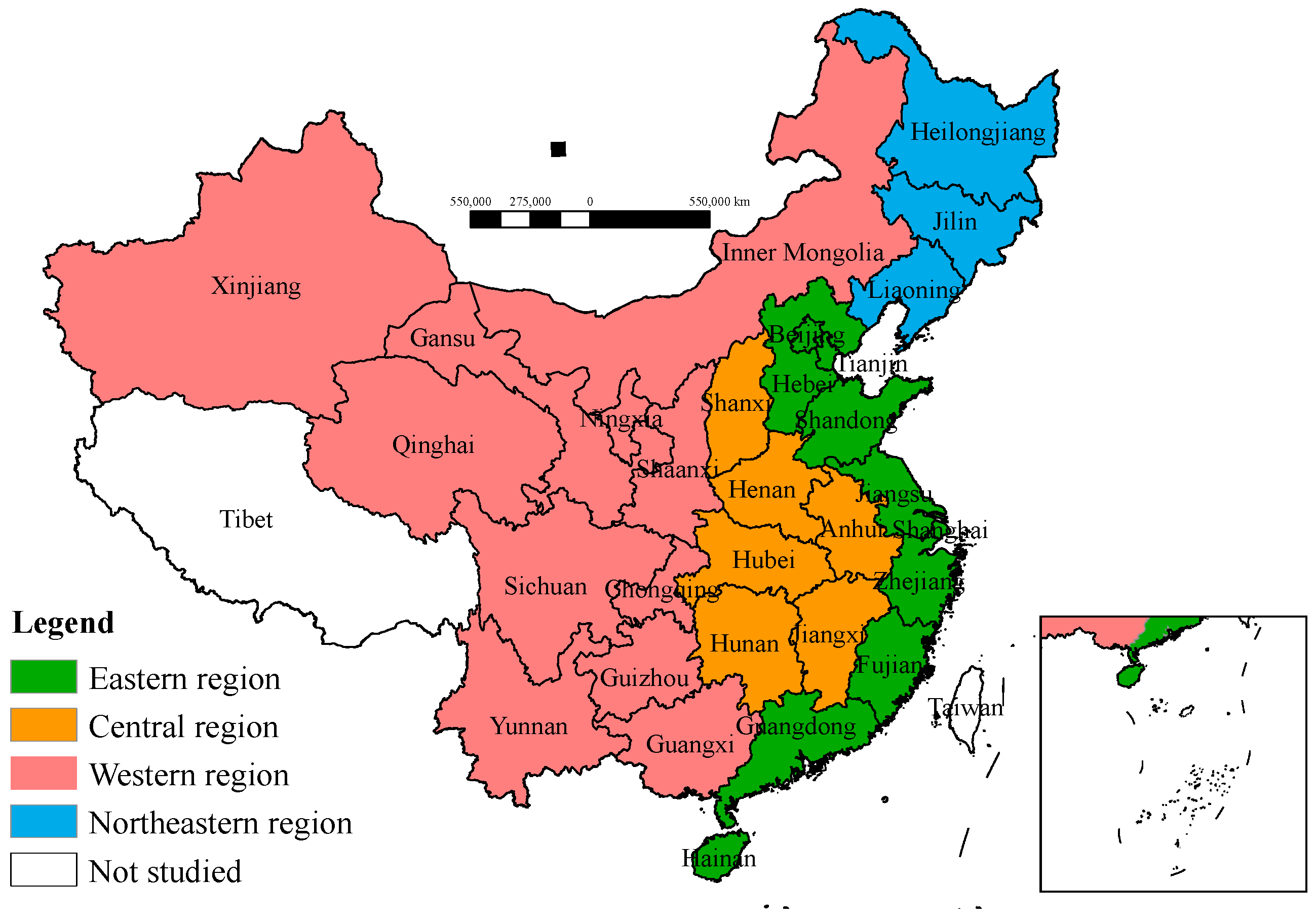
2.6. Data Sources

The dataset in this study encompasses panel data covering the period from 2015 to 2022 for 30 provinces on the Chinese mainland. To guarantee the accuracy and authenticity of the data, the sources utilized include the China Statistical Yearbook (2016–2023), the China Energy Statistical Yearbook (2016–2023), and various provincial statistical yearbooks (2016–2023). The price-related variables addressed in this study, specifically GDP and the value added in the transportation sector, are adjusted to real terms using the provincial GDP deflator and the value-added deflator for the tertiary industry, with 2000 as the base year. Descriptive statistical analyses of the different variables are presented in

Table 2. Descriptive statistics of the different variables.

Variables	Maximum	Minimum	Medium	Average	Standard Deviation	Skewness	Kurtosis	Number
TSCEI	5.6926	0.8278	2.3301	2.4468	0.9018	0.7933	3.5193	210
GDP	3.0578	0.5363	0.9088	1.1197	0.5340	2.0662	7.1152	210
IND	5.2440	0.7510	1.3086	1.4898	0.7709	3.3017	14.6388	210
URB	0.8933	0.4293	0.6099	0.6266	0.1071	0.8429	3.3692	210
TRS	0.7719	0.0149	0.1973	0.2321	0.1527	1.0402	3.8412	210
ENS	0.2055	0.0153	0.0512	0.0631	0.0358	1.7059	5.8618	210
TEC	3.9204	0.4119	1.0264	1.1404	0.5358	2.1425	10.1694	210

. Furthermore, in accordance with the regional classification method of the National Bureau of Statistics of China, the country is divided into eastern, central, western, and northeastern regions, with the provinces included in each region depicted in Figure 1.

3. Empirical Results

3.1. Basic Factual Characteristics: Accounting Results of TSCEI

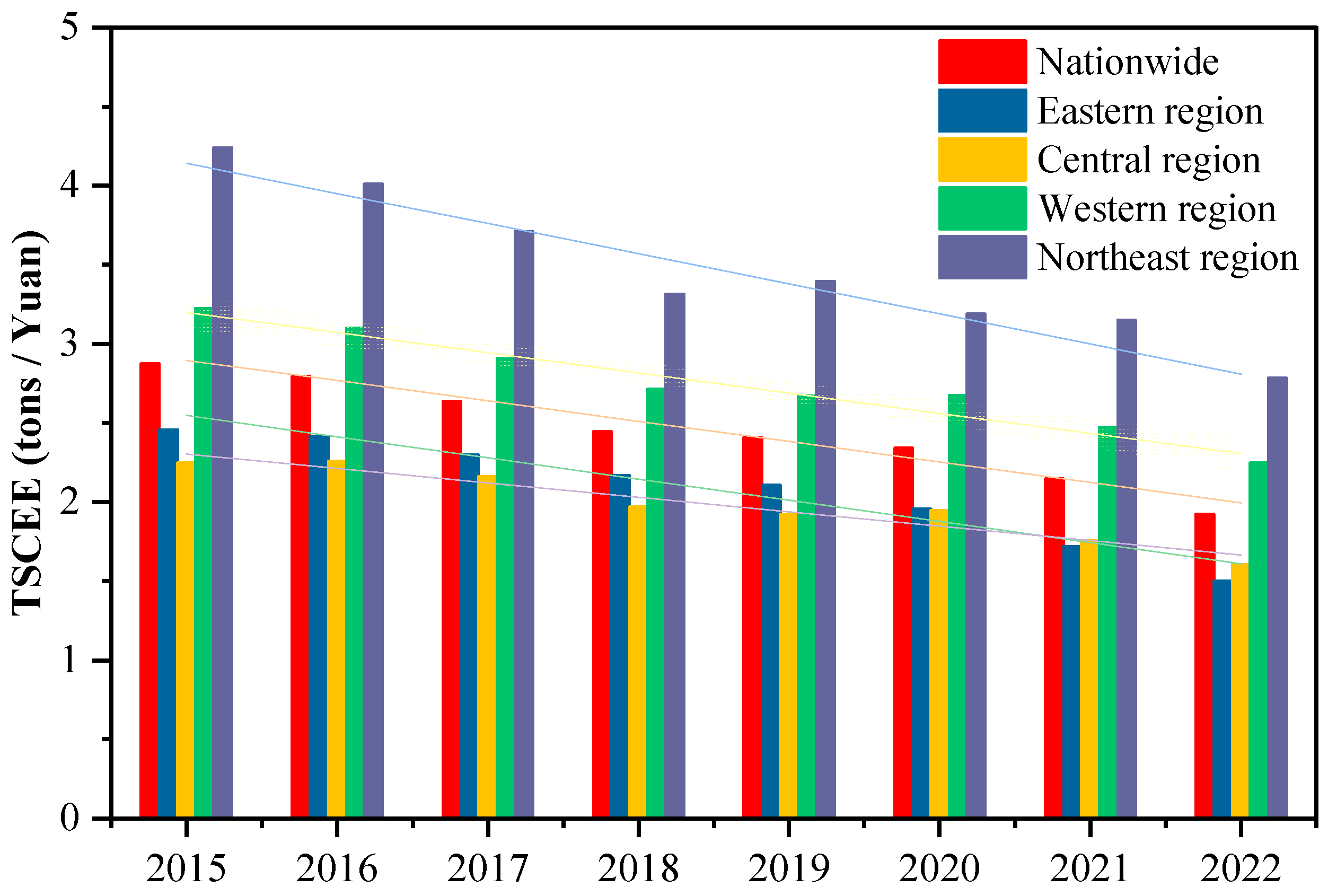
3.1.1. Temporal Evolution of TSCEI in China

Since China announced its carbon peaking target, energy consumption in the transportation sector increased from 328.32 million tons of standard coal in 2015 to 335.14 million tons in 2022, with an average annual growth rate of 0.29%. Correspondingly, carbon emissions from energy consumption rose from 767.89 million tons in 2015 to 813.04 million tons in 2022, at an average annual growth rate of 0.82%. However, TSCEI has decreased from 2.8760 tons per CNY in 2015 to 1.9249 tons per CNY in 2022, with an average of 2.4468 tons per CNY and an annual decline rate of 5.57% (see Figure 2). The decline in TSCEI surpasses the growth rates of both energy consumption and carbon emissions. The trend in TSCEI not only underscores the significant achievements of China’s transportation sector in its low-carbon economic transformation, but also serves as compelling evidence of its commitment to sustainable development.

At the regional level, TSCEI in eastern, central, western, and northeastern China has consistently declined. Specifically, in eastern China, TSCEI decreased from 2.4574 tons per CNY in 2015 to 1.5020 tons per CNY in 2022, reflecting an average annual decline rate of 6.79%. In central China, TSCEI dropped from 2.2466 tons per CNY in 2015 to 1.6064 tons per CNY in 2022, averaging an annual decline rate of 4.68%. In western China, TSCEI was reduced from 3.2271 tons per CNY in 2015 to 2.2489 tons per CNY in 2022, marking an average annual decrease of 5.03%. In northeastern China, TSCEI fell from 4.2430 tons per CNY in 2015 to 2.7836 tons per CNY in 2022, with an average annual decline of 5.84%. The average TSCEI across regions follows this pattern: central China (1.9843 tons per CNY) < eastern China (2.0785 tons per CNY) < western China (2.7532 tons per CNY) < northeastern China (3.4757 tons per CNY). Notably, the TSCEI in the western and northeastern regions is significantly higher than in the eastern and central regions. This disparity underscores the importance of inter-regional collaborative emission reduction efforts. The eastern and central regions should take proactive leadership by exploring and developing replicable and scalable low-carbon practices. Meanwhile, the western and northeastern regions should actively learn from these initiatives and implement stronger transportation emission reduction policies tailored to local conditions.

From the provincial average TSCEI levels (as shown in Figure 3), the four provinces with the lowest TSCEI levels, in ascending order, are Hebei (1.0043), Anhui (1.3729), Henan (1.4291), and Shandong (1.5132), primarily located in the eastern and central regions. Conversely, the provinces with the highest TSCEI levels, in descending order, are Heilongjiang (4.5140), Qinghai (4.0111), Xinjiang (3.7226), and Gansu (3.4450), which are mainly situated in the western and northeastern regions. Among these, Heilongjiang stands out with the highest average TSCEI, accompanied by carbon emissions per unit of economic output in the transportation sector that are far higher than those of other provinces. For instance, this is notable when compared to Hebei Province, which exhibited the lowest average TSCEI, with differences as substantial as a 4.5-fold increase. The disparity in TSCEI levels across provinces creates an uneven playing field for carbon reduction efforts. Without targeted policies that address these spatial inequalities, high-TSCEI provinces may struggle to meet national carbon reduction targets, thereby undermining the overall effectiveness of China’s transportation carbon reduction strategies. This highlights the need for China’s transportation carbon reduction strategies to account for the spatial distribution differences in TSCEI. It also underscores the severe spatial inequality challenges associated with advancing the low-carbon economic transformation within its transportation sector.

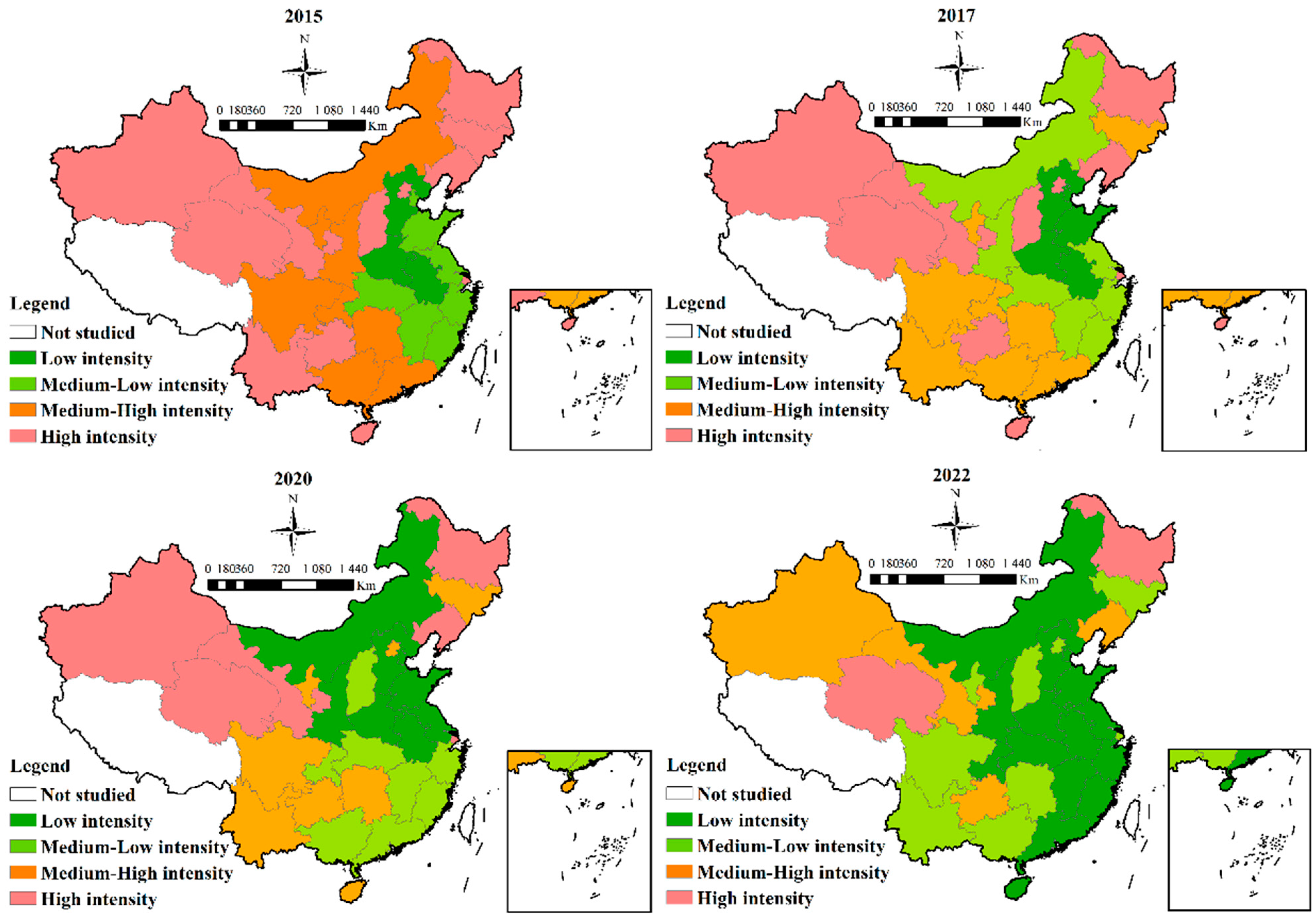
3.1.2. Spatial Distribution Trends of TSCEI in China

To further reveal the spatiotemporal pattern of TSCEI in China, this study employs the trend analysis method and ArcGIS software 10.5 to visualize the spatial distribution trends for 2015, 2017, 2019, 2021, and 2022, as well as the mean value. As depicted in Figure 4, the X-axis is oriented towards the due east, the Y-axis towards the due north, and the Z-axis represents the TSCEI value. The green and blue curves, respectively, illustrate the fitted lines of the TSCEI along the east–west and north–south directions. The blue, green, and red points correspond to the projections of the TSCEI onto the YZ, XZ, and XY planes, respectively.

The trend analysis of TSCEI mean values shows that the spatial distribution of provincial TSCEI follows a “higher in the north, lower in the south; higher in the west, lower in the east” pattern. This observation contrasts sharply with prevailing social-economic development patterns in China, indirectly indicating that regions with stronger economic development tend to have relatively lower TSCEI. Specifically, along the north–south direction, the fitted line for the provincial TSCEI consistently displays a U-shaped pattern over the years, characterized by “low in the middle and high at both ends”. However, this U shape has gradually become less pronounced over time, indicating a decreasing spatial divergence in the TSCEI along the north–south direction across China. Along the east–west direction, the fitted line of TSCEI across provinces also demonstrates a U-shape, though it is less pronounced than in the north–south direction. Furthermore, the fitted line for the central and western regions gradually flattens. Additionally, the downward trend in the TSCEI across China has contributed to the lowering of the trend lines in both the north–south and east–west directions. Overall, the TSCEI in China displays notable spatial heterogeneity.

3.2. Spatial Inequality and Spatial Autocorrelation of TSCEI in China

3.2.1. Measurement and Decomposition of Spatial Differences of TSCEI in China

The study further utilizes the Dagum Gini coefficient to quantitatively assess the extent and causes of spatial inequality in TSCEI across China. The detailed results are provided in

Table 3. The measurement of spatial differences in TSCEI.

Year	Overall Differences	Intra-regional Differences				Inter-Regional Differences
		E	C	W	N	E-C	E-W	E-N	C-W	C-N	W-N
2015	0.1966	0.2041	0.1382	0.1268	0.1401	0.1866	0.2039	0.2874	0.2037	0.3133	0.1805
2016	0.1971	0.1958	0.1457	0.151	0.1475	0.1825	0.2041	0.275	0.2001	0.2875	0.1854
2017	0.1884	0.2006	0.1279	0.1398	0.129	0.1737	0.2015	0.2641	0.1857	0.271	0.1704
2018	0.1763	0.1767	0.1343	0.1341	0.1186	0.1707	0.1822	0.2351	0.1857	0.2602	0.1567
2019	0.1853	0.1837	0.142	0.1381	0.1228	0.1783	0.1911	0.2562	0.1914	0.2777	0.1689
2020	0.1886	0.1849	0.1258	0.1585	0.1078	0.1661	0.2102	0.2562	0.1929	0.2459	0.1597
2021	0.1972	0.1762	0.1302	0.1507	0.1229	0.1642	0.221	0.3048	0.1976	0.2868	0.1753
2022	0.1958	0.1417	0.1377	0.1558	0.1488	0.1498	0.223	0.3098	0.1998	0.2806	0.1867
Average	0.1907	0.1830	0.1352	0.1444	0.1297	0.1715	0.2046	0.2736	0.1946	0.2779	0.1730

Note: E, C, W and N represent the eastern, central, western and northeastern regions of China, respectively.

and

Table 4. Decomposition of the overall differences in TSCEI.

Year	Overall Differences	Intra-Regional Differences		Inter-Regional Differences		Transvariation Density
		Source	Contribution (%)	Source	Contribution (%)	Source	Contribution (%)
2015	0.1966	0.0449	22.84	0.1101	56.02	0.0416	21.14
2016	0.1971	0.0482	24.43	0.0992	50.30	0.0498	25.27
2017	0.1884	0.0462	24.51	0.0935	49.60	0.0488	25.90
2018	0.1763	0.0434	24.61	0.0906	51.37	0.0423	24.02
2019	0.1853	0.0448	24.16	0.0977	52.74	0.0428	23.11
2020	0.1886	0.0472	25.01	0.0967	51.30	0.0447	23.69
2021	0.1972	0.0451	22.88	0.1154	58.52	0.0367	18.60
2022	0.1958	0.0435	22.22	0.1201	61.35	0.0322	16.43
Average	0.1907	0.0454	23.83	0.1029	53.90	0.0424	22.27

.

Regarding intra-regional differences, the overall TSCEI differences show an initial decline followed by an increase, decreasing slightly from 0.1966 in 2015 to 0.1958 in 2022, with an average of 0.1907. This reflects significant overall differences, mainly due to the unbalanced and insufficient development in China’s low-carbon transportation sector. The transition to low-carbon transportation varies significantly across provinces. Notably, both the eastern and central regions exhibit a trend of decreasing intra-regional differences, declining from 0.2041 and 0.1382 in 2015 to 0.1417 and 0.1377 in 2022, respectively. In contrast, the western and northeastern regions experienced a fluctuating increase, rising from 0.1268 and 0.1401 in 2015 to 0.1558 and 0.1488 in 2022, respectively. The average intra-regional differences follow this pattern: eastern region (0.1830) > western region (0.1444) > central region (0.1352) > northeastern region (0.1297). This pattern is primarily attributed to the significant variations in TSCEI in the eastern region, while TSCEI levels among provinces in the other regions remain relatively consistent. Furthermore, the average values of inter-regional differences, ranked from largest to smallest, are as follows: central–northeast (0.2779), east–northeast (0.2736), east–west (0.2046), central–west (0.1946), west–northeast (0.1730), and east–central (0.1715). Notable inter-regional differences exist between the northeast and both the eastern and central regions.

The decomposition results of overall differences reveal that the average values of $G_w$, $G_{nb}$, and $G_t$ are 0.0454, 0.1029, and 0.0424, respectively, with corresponding average contribution rates of 23.83%, 53.90%, and 22.27%, respectively. This indicates that inter-regional differences are the primary contributors to the overall TSCEI differences in China, followed by intra-regional differences and transvariation density. Regarding contribution trends, the contribution rate from intra-regional differences remains relatively stable, while the contribution rate of transvariation density exhibits a declining trend. Transvariation density reflects the contribution of cross-regional overlap to the overall differences. Its low contribution rate suggests that dividing regions into four groups effectively distinguishes different provinces. Additionally, the contribution rate of inter-regional differences increased from 56.02% in 2015 to 61.35% in 2022, indicating a marked growth trend. This underscores the importance of reducing inter-regional differences, especially between the northeast and the east and central regions, as a crucial focus for China’s transportation carbon emission reduction efforts in the coming years.

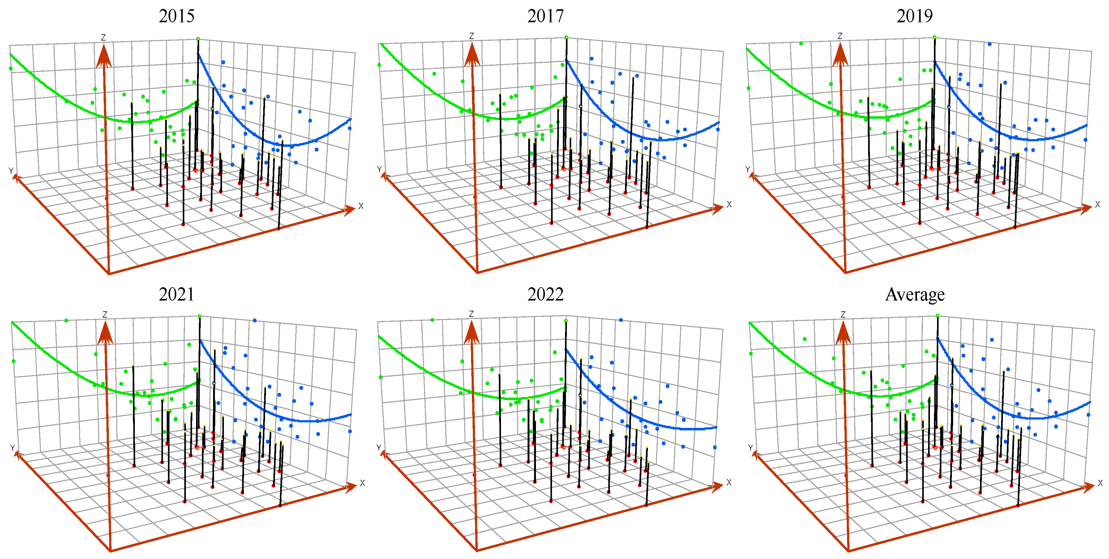
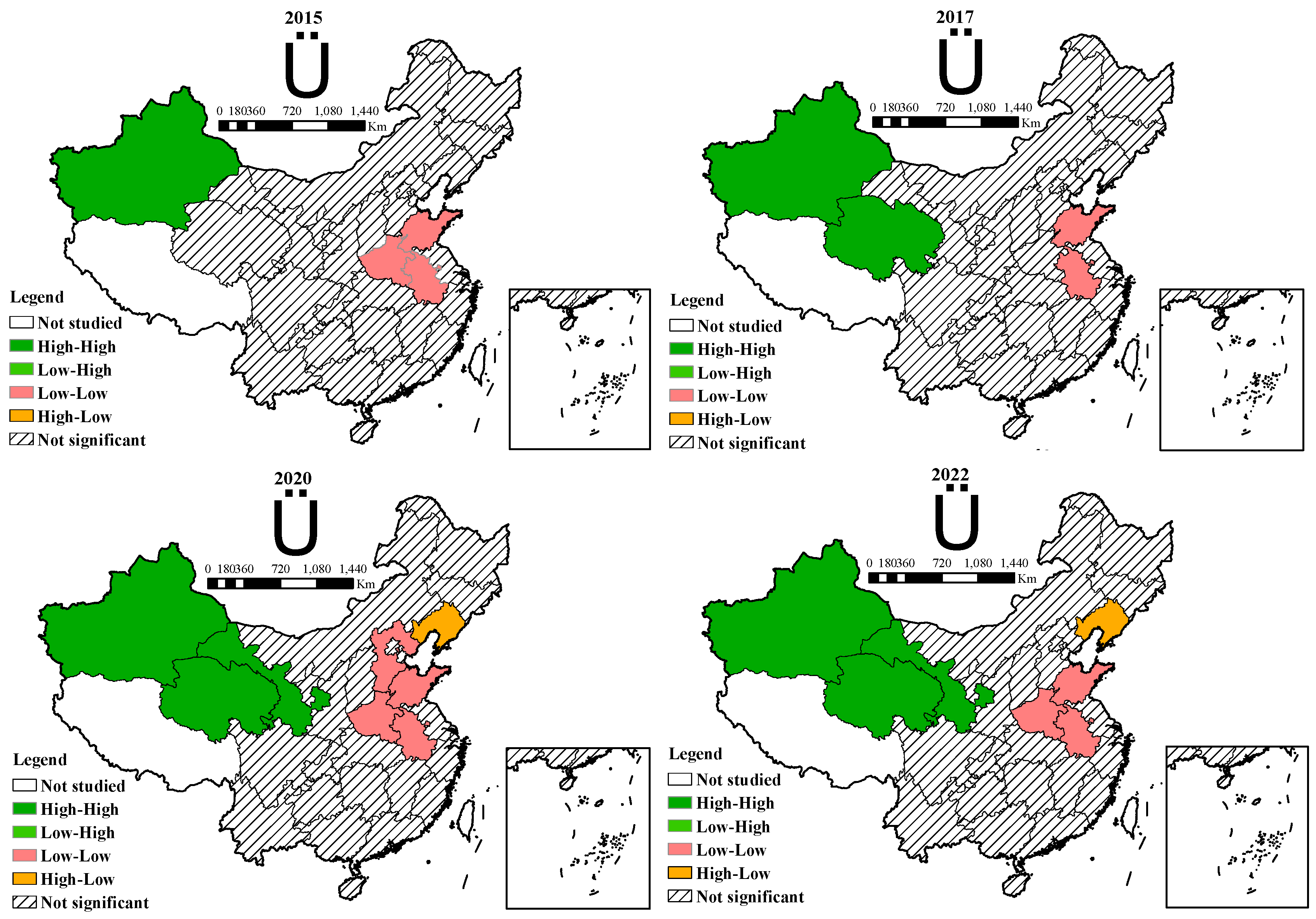
3.2.2. Spatial Autocorrelation Analysis of TSCEI in China

Using Stata 17 software, the study calculates the global Moran’s I index of TSCEI in China under the first-order Rook contiguity spatial weights matrix. As depicted in

Table 5. The global Moran’s I index of TSCEE in 2010–2022.

	2015	2016	2017	2018	2019	2020	2021	2022
Moran’ I	0.2018	0.1702	0.1833	0.2100	0.1925	0.3197	0.3084	0.2868
E(I)	−0.0345	−0.0345	−0.0345	−0.0345	−0.0345	−0.0345	−0.0345	−0.0345
Sd(I)	0.1215	0.1236	0.1227	0.1228	0.1221	0.1220	0.1218	0.1202
Z-score	1.9458	1.6560	1.7748	1.9914	1.8589	2.9023	2.8147	2.6718
p-value	0.0517 *	0.0977 *	0.0759 *	0.0464 **	0.0630 *	0.0037 ***	0.0049 ***	0.0075 ***

Note: *, **, *** indicate significance at the 10%, 5%, and 1% levels, respectively.

, the global Moran’s I index for provincial TSCEI maintained positive values throughout the study period, with p-values meeting the 10% significance level threshold. These findings imply spatial dependence in the distribution of TSCEI. Furthermore, the global Moran’s I index generally displays an upward trajectory, suggesting an increasing degree of spatial correlation in TSCEI among provinces.

To analyze the local spatial agglomeration of provincial TSCEI in China, Figure 5 shows the LISA agglomeration maps for 2015, 2017, 2020, and 2022 at the 10% significance level. In 2015, 2017, 2020, and 2022, 13.33%, 13.33%, 23.33%, and 20.00% of the provinces exhibited significant spatial agglomeration, respectively. Specifically, in 2015, the numbers of provinces in the H-H, H-L, L-L, and L-H categories were 1, 0, 3, and 0, respectively. In 2017, the corresponding numbers were 2, 0, 2, and 0. In 2020, the numbers were 3, 0, 4, and 1, and in 2022, they were 3, 0, 3, and 1. Provinces showing H-H and L-L types in 2015, 2017, 2020, and 2022 accounted for 100%, 100%, 87.50%, and 85.71% of the significant provinces, respectively. The findings reveal that the significant local spatial correlation of TSCEI among provinces in China is predominantly characterized by H-H and L-L types, indicating a strong positive spatial agglomeration pattern. Specifically, in 2015, provinces classified as H-H type included Xinjiang, while L-L type provinces included Anhui, Shandong, and Henan. By 2017, the H-H type expanded to include Xinjiang and Qinghai, while the number of L-L type provinces decreased to just Anhui and Shandong. By 2020, the H-H type further extended to Xinjiang, Qinghai, and Gansu, while the L-L type expanded to include Hebei, Anhui, Shandong, and Henan. In 2022, relative to 2020, the provinces classified as H-H type remained constant, while the L-L type provinces reduced to only Anhui, Shandong, and Henan. Geographically, provinces exhibiting L-L agglomeration are mainly concentrated in eastern and central China, while those in the H-H agglomeration type are predominantly located in western regions. Therefore, Hebei, Anhui, Henan, and Shandong not only demonstrate strong performance regarding TSCEI control, but are also identified as the L-L agglomeration type. This highlights the need to enhance the spatial diffusion effect of TSCEI in eastern and central provinces, reducing overall TSCEI levels and promoting low-carbon development in China.

3.3. Evolutionary Trend Forecasting of TSCEI in China

To reveal the evolutionary trend of TSCEI in China, this study employs the quantile method to classify the full sample into four types: low intensity ($0<TSCEI\le 1.7744$), medium–low intensity ($1.7744<TSCEI\le 2.3301$), medium–high intensity ($2.3301<TSCEI\le 2.9028$), and high intensity ($2.9028<TSCEI\le 5.6926$). Using ArcGIS software 10.5, this study generates TSCEI distribution maps for the years 2015, 2017, 2020, and 2022, which provide a visual representation of the evolution trend of provincial TSCEI, as shown in Figure 6. The data indicate an upward trend in the number of provinces classified as low and medium–low intensity, increasing from 3 and 7 in 2015 to 15 and 9 in 2022, respectively. Conversely, the number of medium–high- and high-intensity provinces declined, from 8 and 12 in 2015 to 4 and 2 in 2022, respectively. The proportion of provinces classified as low, medium–low, medium–high, and high intensity shifted from 10.00%, 23.33%, 26.67%, and 40.00% in 2015 to 50.00%, 30.00%, 13.33%, and 6.67% in 2022, respectively. Significant changes have occurred in the spatial distribution of provincial TSCEI in China throughout the study period. Specifically, in 2015, only Hebei, Anhui, and Henan were classified as low intensity. By 2022, the low-intensity provinces expanded significantly, while the number of high-intensity provinces decreased to only Heilongjiang and Qinghai. The medium–high intensity category was limited to four provinces: Liaoning, Guizhou, Gansu, and Xinjiang. Notably, the medium–high- and high-intensity provinces are concentrated primarily in the western and northeastern regions.

3.3.1. Dynamic Transfer Trend of TSCEI in China

This study further explores the dynamic transfer trends of TSCEI in China by applying the Markov chain method.

Table 6. Traditional Markov transfer probability matrix for TSCEI.

Type	N	1	2	3	4
1	45	0.8791	0.1209	0.0000	0.0000
2	51	0.1556	0.7556	0.0889	0.0000
3	56	0.0000	0.1348	0.7640	0.1011
4	58	0.0000	0.0000	0.1333	0.8667

presents the traditional Markov transfer probability matrix. Based on the calculation results, several key observations can be drawn. First, the state transfers of provincial TSCEI demonstrate stability. The probabilities of maintaining the current state, as indicated by the diagonal elements of the matrix, are significantly higher than those of transferring to other states, as indicated by the off-diagonal elements. Notably, the minimum value among the diagonal elements is 0.7556, indicating that TSCEIs across provinces have at least a 75.56% probability of remaining in their current states in the subsequent year. Provinces classified under low and high intensity types exhibit greater stability, with probabilities of retaining their current states of 87.91% and 86.67%, respectively. Second, the probability of downward transfer is higher than that of upward transfer. For example, the transfer probability from the middle–low- to the low-intensity state, denoted as $P_{21}=0.1556$, exceeds that of the transfer to the middle–high-intensity state, $P_{23}=0.0889$. Similarly, the transfer probability from the middle–high- to the middle–low-intensity state, $P_{32}=0.1348$, exceeds that of the transfer to a high intensity state, $P_{34}=0.1011$, indicating a trend toward further evolution to lower intensity levels of TSCEI in China. Third, the leapfrog state transfer of TSCEI is notably difficult to achieve. All state transfers occur between adjacent states, with zero probability for leapfrog shifts.

Given that traditional Markov matrices do not account for neighboring states’ influences, this study extends the framework by incorporating spatial lag effects, constructing a spatial Markov chain model. To verify the statistical significance of these spatial lag effects, the hypothesis test conducted in this study reveals the following: At a significance level of $\alpha =0.005$, the computed likelihood ratio statistic $Q>{\chi }^2(40)=66.77$, with a p-value of 0.0000. Thus, the null hypothesis, which posits that the state transfers of the TSCEI are spatially independent and unrelated to the state types of neighboring provinces, can be rejected. This finding suggests that the upward or downward transfer of TSCEI is not spatially isolated, but rather exhibits significant interdependencies with neighboring provinces. The spatial Markov transfer probability matrix is presented in

Table 7. Spatial Markov transfer probability matrix for TSCEE.

Neighborhoods	Type	N	1	2	3	4
1	1	17	1.0000	0.0000	0.0000	0.0000
	2	6	0.5000	0.5000	0.0000	0.0000
	3	5	0.0000	0.6000	0.4000	0.0000
	4	12	0.0000	0.0000	0.2500	0.7500
2	1	22	0.9545	0.0455	0.0000	0.0000
	2	30	0.2667	0.7000	0.0333	0.0000
	3	9	0.0000	0.4444	0.5556	0.0000
	4	14	0.0000	0.0000	0.0714	0.9286
3	1	6	1.0000	0.0000	0.0000	0.0000
	2	12	0.1667	0.7500	0.0833	0.0000
	3	30	0.0000	0.2333	0.7667	0.0000
	4	13	0.0000	0.0000	0.2308	0.7692
4	1	0	0.0000	0.0000	0.0000	0.0000
	2	3	0.0000	1.0000	0.0000	0.0000
	3	12	0.0000	0.1667	0.8333	0.0000
	4	19	0.0000	0.0000	0.1579	0.8421

.

By comparing Table 6 and Table 7, the following observations emerge: First, geospatial patterns significantly influence TSCEI evolution in China. Under varying neighborhood states, the transfer probabilities of TSCEI vary, deviating from the traditional Markov transfer probability matrix. For instance, when geospatial patterns are not considered, the probability $P_{12}=0.1209$, whereas, when a province is adjacent to provinces with medium–low intensity, $P_{12}(2)=0.0455$. This suggests that analyzing the dynamic transfer trend of TSCEI in China, while accounting for spatial lag effects, is crucial. Second, under the influence of geospatial patterns, the probabilities of state transfers in TSCEI differ depending on the type of neighboring provinces. For example, in the case of downward transfers, $P_{21}(1)=0.5000$ > $P_{21}(2)=0.2667$ > $P_{21}(3)=0.1667$ > $P_{21}=0.1556$; similarly, $P_{32}(1)=0.6000$ > $P_{32}(2)=0.4444$ > $P_{32}(3)=0.2333$ > $P_{32}(4)=0.1667$ > $P_{32}=0.1348$. In contrast, for upward transfers, $P_{12}(1)=0$ < $P_{12}(2)=0.0455$ < $P_{12}=0.1209$; and $P_{23}(1)=0$ < $P_{23}(2)=0.0333$ < $P_{23}(3)=0.0833$ < $P_{23}=0.0899$. Evidently, the probability of downward transfer increases when a province is adjacent to provinces with lower TSCEI levels, whereas upward transfers are more probable when neighboring provinces exhibit higher TSCEI levels. Third, similar to the traditional Markov transfer probability matrix, the diagonal elements correspond to higher probabilities than the non-diagonal elements, with state transfers occurring between adjacent states in the spatial Markov transfer probability matrix. This indicates that, even under the influence of spatial lag effects, the state transfers of TSCEI remain stable, with leapfrog shifts being highly improbable.

The preceding analysis demonstrates that geospatial patterns significantly influence the spatiotemporal evolution of TSCEI in China, displaying distinct spatial spillover effects. Specifically, provinces with lower TSCEI levels tend to facilitate downward transfer in neighboring provinces, thereby exhibiting positive spillover effects. Conversely, provinces with higher TSCEI levels tend to restrain downward transfer in neighboring provinces, thereby demonstrating negative spillover effects. However, the positive inter-province spillover effects on the improvement of lagged provinces are relatively limited. Consequently, it is essential for the formulation of low-carbon transportation policies to account for the potential to leverage positive spillover effects, thus contributing to the overall improvement of TSCEI in China.

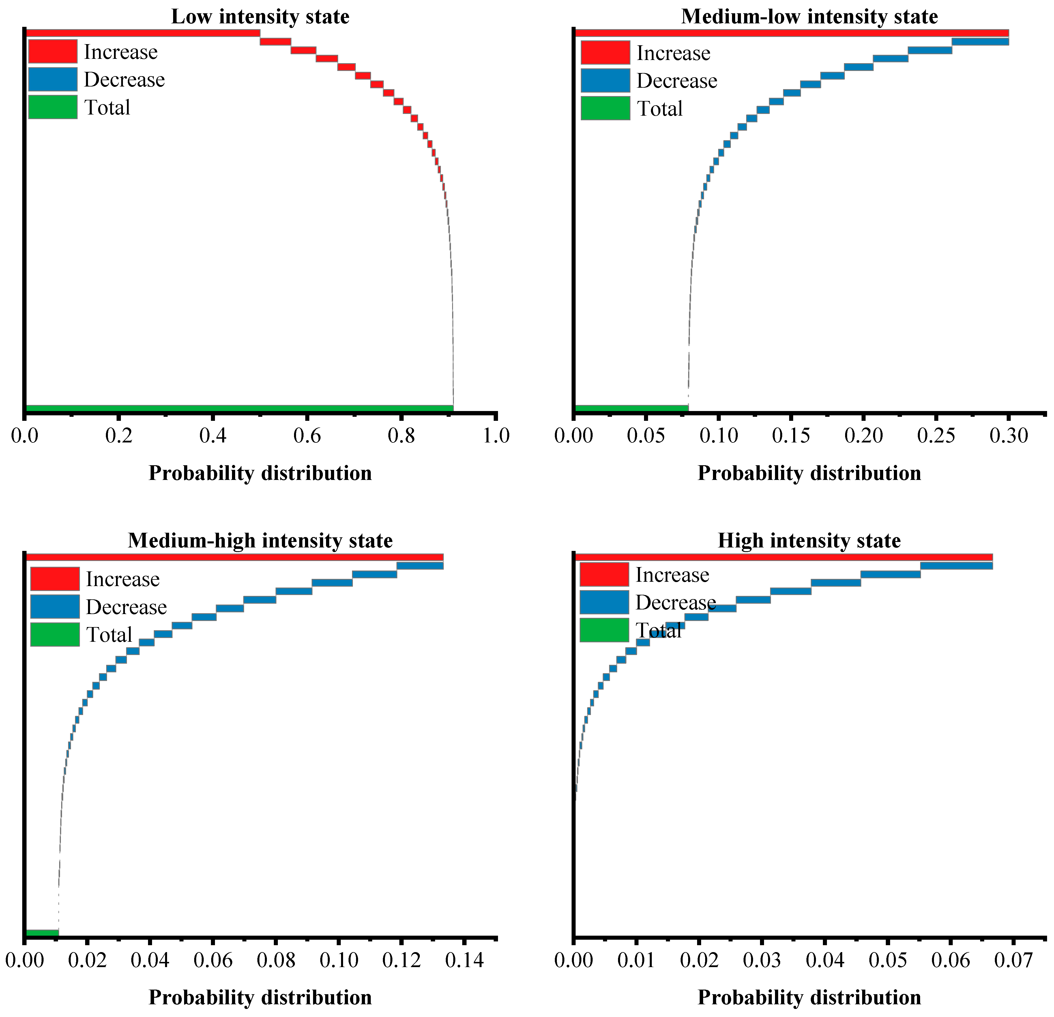
3.3.2. Future Trend Forecasting of TSCEI in China

Due to the inherent stability of TSCEI in maintaining its current state, the state transfer process has not yet reached an equilibrium or ultimate state. Thus, the state transfer process of TSCEI will continue to evolve. By calculating the limiting distributions of both traditional and spatial Markov processes, the future evolutionary trend of TSCEI in China can be effectively forecasted. Following each state transfer, the probability distributions of the various states of TSCEI for the subsequent year can be determined. When $k\to \infty$, the ultimate state probability distribution for various states of TSCEI, after $k$ shifts, can be determined.

Without considering spatial lags, a comparison between the ultimate state probabilities (as shown in Figure 7 and

Table 8. Ultimate evolution state prediction of TSCEI.

			I	II	III	IV
	Initial state (Year = 2022)		0.5000	0.3000	0.1333	0.0667
No ${\omega }_{ij}$	Ultimate state (Year$\to \infty$)		0.9098	0.0793	0.0109	0.0000
Consider ${\omega }_{ij}$	Ultimate state (Year$\to \infty$)	I	1.0000	0.0000	0.0000	0.0000
		II	0.8451	0.1441	0.0108	0.0000
		III	1.0000	0.0000	0.0000	0.0000
		IV	0.0000	1.0000	0.0000	0.0000

) and the initial state probabilities reveals a significant decrease in the number of provinces in the medium–low- and medium–high-intensity states, with no provinces in the high-intensity state. Conversely, the number of provinces in the low-intensity state has significantly increased. Specifically, under the premise of maintaining current policies, the distributions of ultimate state probabilities for the low-, medium–low-, medium–high-, and high-intensity states are 90.98%, 7.93%, 1.09%, and 0%, respectively. When accounting for spatial lags, the limiting probability distribution of the TSCEI exhibits significant differences under various geospatial patterns, in contrast to the limiting probability distribution without spatial lags. In the long term, when adjacent to provinces in the low-intensity state, the probability of a province being in the low-intensity state is 100%. Similarly, when adjacent to medium–low-intensity provinces, the probabilities of transferring to the low-, medium–low-, and medium–high-intensity states are 84.51%, 14.41%, and 1.08%, respectively. When adjacent to provinces with medium–high or high intensities, the probabilities of the TSCEI states being in the low-intensity or medium–low-intensity state are both 100%. Overall, under the current development trajectory, TSCEI tends to shift from high- to low-intensity states over time, regardless of spatial lags. The long-term trend of the TSCEI is expected to continue its decline, and the influence of neighboring states on the evolution of the TSCEI exhibits significant heterogeneity.

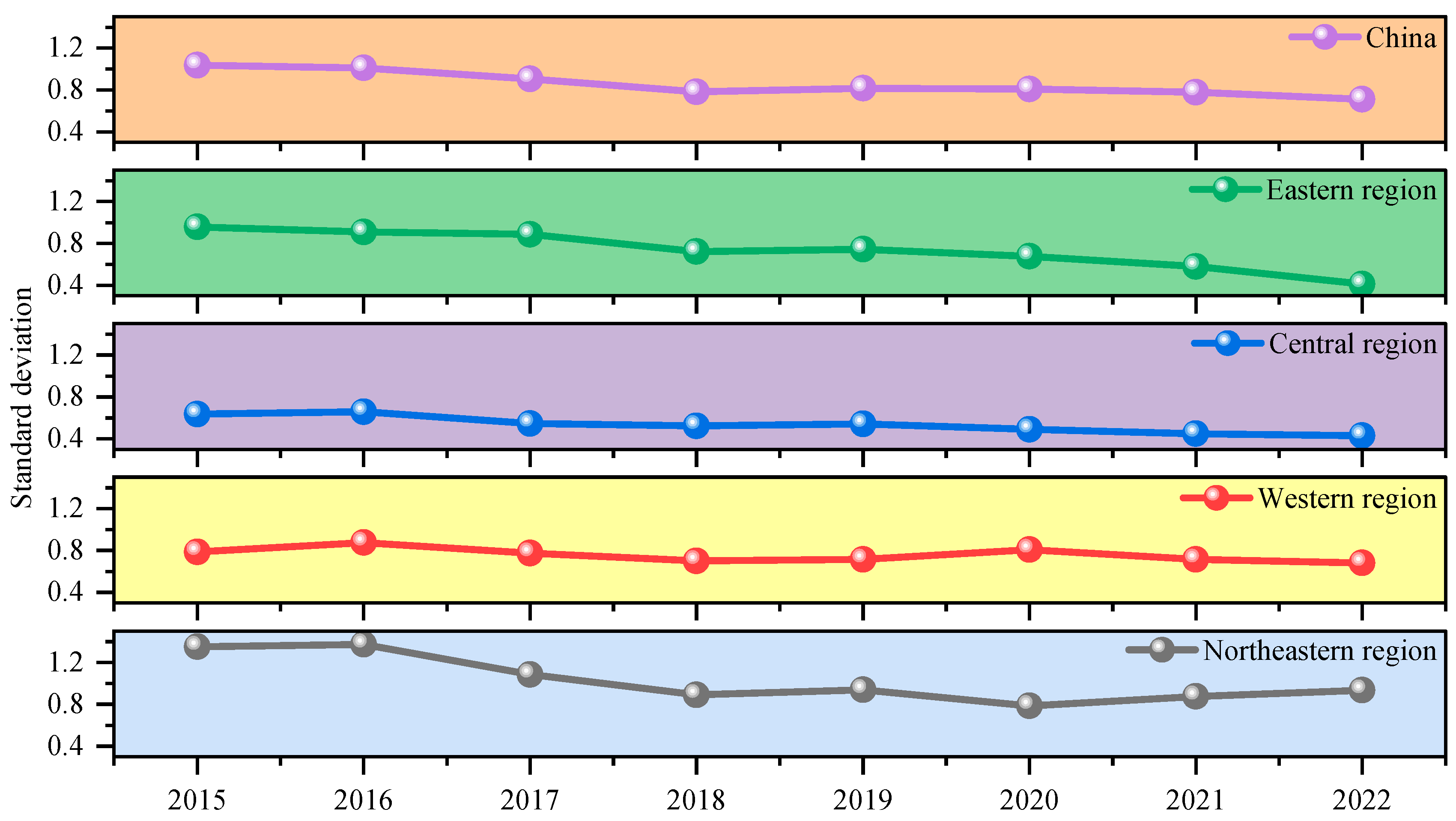
3.4. Spatial Convergence Analysis of TSCEI in China

3.4.1. $\sigma$ Convergence Analysis of TSCEI in China

Figure 8 and

Table 9. $\sigma$ convergence test of TSCEI: 2015–2022.

	China	Eastern Region	Central Region	Western Region	Northeastern Region
_Cons	1.0545 ***	1.0609 ***	0.0670 ***	0.8329 ***	1.3643 ***
	(31.34)	(32.97)	(26.91)	(20.35)	(13.38)
$\xi$	−0.0441 ***	−0.0715 ***	−0.0314 ***	−0.0168 *	−0.0746 **
	(−8.76)	(−8.98)	(−8.54)	(−2.42)	(−3.50)
R2	0.8518	0.9365	0.8941	0.3942	0.6761

Note: values in parentheses are t-values. *, **, *** indicate significance at the 10%, 5%, and 1% levels, respectively.

present the convergence results and significance tests for TSCEI at national and regional levels. At the national level, the standard deviation of TSCEI decreased from 1.0380 in 2015 to 0.7102 in 2022, reflecting a $\sigma$ convergence pattern with an average annual decline rate of 5.28%. Econometric analyses further indicate a negative time trend coefficient $\xi$ that is statistically significant at the 1% level, suggesting a clear trend of reduced TSCEI dispersion in China. Regionally, the standard deviations for the eastern, central, western, and northeastern regions fell from 0.9590, 0.6368, 0.7874, and 1.3515 in 2015 to 0.4137, 0.4311, 0.6820, and 0.9340 in 2022, respectively. The annual average decline rates for these regions were 11.32%, 5.42%, 2.03%, and 5.14%. Meanwhile, the time trend coefficients $\xi$ for all four regions are negative and statistically significant. In general, the degree of dispersion in TSCEI across China and its four regions has decreased over time, demonstrating the characteristic of $\sigma$ convergence.

3.4.2. Absolute $\beta$ Convergence Analysis of TSCEI in China

Table 10. Absolute $\beta$ convergence test of TSCEI.

	China	Eastern Region	Central Region	Western Region	Northeastern Region
Mode type	SDM	SDM	SEM	OLS	SAR
$\beta$	−0.4595 ***	−0.4954 ***	−0.4169 ***	−0.4989 **	−0.4420 **
	(−8.14)	(−4.05)	(−4.80)	(−3.04)	(−2.41)
$\rho /\lambda$	0.1667 *	0.2450 **	0.0443	—	−0.3537 *
	(1.90)	(2.23)	(0.25)		(−1.84)
$\upsilon$ (%)	0.0879	0.0977	0.0771	0.0987	0.0833
LM-Error	18.109 ***	18.791 ***	11.237 ***	0.847	4.962 **
Robust-LM-Error	5.307 **	4.401 **	1.661	0.747	0.686
LM-Lag	17.175 ***	17.397 ***	11.081 ***	0.816	4.969 **
Robust-LM-Lag	4.374 **	3.008 *	1.505	0.716	0.693 **
Time-fixed	Yes	Yes	Yes	Yes	Yes
Individual-fixed	Yes	Yes	Yes	Yes	Yes
Hausman	62.53 ***	14.06 ***	12.68 ***	7.96 ***	6.37 **
R2	0.0982	0.1130	0.0172	0.4256	0.0351

*, **, *** indicate significance at the 10%, 5%, and 1% levels, respectively.

presents the absolute $\beta$ convergence results for national and regional TSCEI, along with the corresponding annual convergence rates. To determine the optimal econometric model specification, this study first employs the LM test and the Robust-LM test to assess whether TSCEI exhibits spatial autocorrelation effects. Subsequently, the Wald test and LR test are used to determine whether the SDM model can be simplified into the SAR and SEM models. The Hausman test is applied to determine whether the econometric model should adopt random effects or fixed effects. Based on this decision, the AIC and BIC criteria are then used to determine whether to adopt individual fixed effects, time fixed effects, or individual–time fixed effects.

The results suggest a clear trend of an absolute $\beta$ convergence trend in TSCEI at both the national and regional levels. Specifically, at the 1% confidence level, significant negative convergence is observed in the national, eastern, and central regions, while the western and northeastern regions exhibit significant negative convergence at the 5% confidence level. This indicates that, without other influencing factors, TSCEI will converge to a uniform steady-state level over time. Moreover, the speed of absolute $\beta$ convergence varies across regions. The national $\beta$ convergence rate is 0.0879, while the western and eastern regions, with rates of 0.0987 and 0.0977, respectively, converge faster than the national average. In contrast, the northeastern and central regions, with rates of 0.0833 and 0.0771, respectively, experience slower convergence. Additionally, there are regional differences in spatial effects. Both the national and eastern regions exhibit significant positive spatial lag effects in both the explanatory and dependent variables at the 10% and 5% confidence levels, respectively, indicating that TSCEI changes in one province positively influence TSCEI changes in neighboring provinces, reflecting a spatial spillover effect. However, the central and northeastern regions display spatial error lags and dependent variable lags, respectively. The western region, in contrast, shows no significant spatial effects, making it suitable for conducting the absolute $\beta$ convergence test using a traditional fixed-effects panel model. It is important to note that the absolute $\beta$ convergence analysis assumes that factors such as per capita GDP, industrial structure, urbanization rate, transportation infrastructure, transportation energy structure, and technological progress are uniform across regions. However, this assumption is often unrealistic. Therefore, this study introduces control variables to perform a conditional $\beta$ convergence test.

3.4.3. Conditional $\beta$ Convergence Analysis of TSCEI in China

Following the optimal econometric model testing procedure for absolute $\beta$ convergence,

Table 11. Conditional $\beta$ convergence test of TSCEI.

	China	Eastern Region	Central Region	Western Region	Northeastern Region
Mode type	SEM	OLS	OLS	OLS	OLS
$\beta$	−0.9666 ***	−0.9815 ***	−0.9167	−0.9807 ***	−0.7901 ***
	(−50.45)	(−30.47)	(−64.43)	(−28.87)	(−6.69)
$\rho /\lambda$	0.3711 ***	—	—	—	—
	(4.14)
GDP	−0.0718	0.0529	0.0335	0.2248	0.3014
	(−1.08)	(0.42)	(0.47)	(1.10)	(0.77)
IND	−0.0694 **	−0.1799 *	−0.0318	−0.0755	−0.0326
	(−2.54)	(−2.19)	(−1.18)	(−0.90)	(−0.15)
URB	0.1827 *	0.6070	0.1628	0.7938 **	−0.9203
	(1.89)	(1.50)	(0.50)	(2.42)	(−1.46)
TRS	−0.0002	0.0026	0.0140	−0.0042	−0.0222
	(−0.03)	(0.13)	(0.83)	(−0.20)	(−0.50)
ENS	−0.1282 ***	−0.1114 *	−0.1807 ***	−0.1406 ***	−0.1736 ***
	(−11.67)	(−2.46)	(−12.81)	(−4.00)	(−6.61)
TEC	−0.9215 ***	−0.9185 ***	−1.0335 ***	−0.9627 ***	−1.0548 ***
	(−41.55)	(−15.98)	(−52.21)	(−19.82)	(−21.08)
$\upsilon$ (%)	0.4856	0.5700	0.3550	0.5640	0.2230
LM-Error	28.715 ***	0.079	0.132	0.000	0.088
Robust-LM-Error	28.882 ***	2.528	0.037	1.025	0.855
LM-Lag	1.724	10.563 ***	0.981	4.017 **	2.045
Robust-LM-Lag	1.891	13.012 ***	0.886	5.042 **	2.812 *
Time-fixed	Yes	Yes	Yes	Yes	No
Individual-fixed	Yes	Yes	Yes	Yes	No
Hausman	42.08 ***	40.07 ***	16.72 ***	32.48 ***	0.85
R2	0.8938	0.9730	0.9919	0.9567	0.9571

*, **, *** indicate significance at the 10%, 5%, and 1% levels, respectively.

presents the results of conditional $\beta$ convergence and the corresponding convergence rates for the national and regional TSCEI. The findings indicate that, first, the convergence coefficient $\beta$ is statistically significant at the 1% confidence level for both the national and regional levels, indicating the presence of conditional $\beta$ convergence. This means that, even after controlling for heterogeneity factors such as per capita GDP, industrial structure, urbanization rate, transportation structure, transportation energy structure, and technological progress, TSCEI will converge towards its respective steady-state level at both national and regional levels. Second, compared to absolute $\beta$ convergence, the conditional $\beta$ convergence rates at both the national and regional levels have accelerated. Specifically, the convergence rates for the national, eastern, central, western, and northeastern regions increased from 0.0879, 0.0977, 0.0771, 0.0987, and 0.0833 under absolute $\beta$ convergence to 0.4856, 0.5700, 0.3550, 0.5640, and 0.2230 under conditional convergence, respectively. This demonstrates the reasonableness of the selected control variables. Third, compared to the absolute $\beta$ convergence test, the spatial effects at the national and regional levels show significant changes. The national conditional $\beta$ convergence analysis shifted from the SDM model to the SEM model, with a significantly positive $\lambda$ at the 1% confidence level. In addition, traditional panel data models are deemed suitable for conducting conditional $\beta$ convergence analysis in the four regions.

From an economic perspective, significant differences exist in the magnitude and significance of the coefficients of control variables affecting the TSCEI change rate at both national and regional levels. At the national level, industrial structure, transportation energy structure, and technological progress have a significantly negative impact on the TSCEI change rate. This suggests that optimizing the industrial structure towards services and non-manufacturing industries, decarbonizing the energy structure by transitioning to electricity, and advancing low-carbon transport technologies that focus on enhancing sustainability by consuming less energy per unit of output, can effectively promote the convergence of TSCEI to lower values. In contrast, the urbanization rate significantly positively impacts the TSCEI change rate. Meanwhile, per capita GDP and transportation structure do not exert a significant influence. This absence of statistical significance does not imply that advancements in economic prosperity and the improvement of transportation structure are inconsequential to TSCEI. Instead, it suggests that these factors do not play a decisive role in propelling TSCEI towards either increased or decreased levels of convergence. Examining the regional level, the optimization of the industrial structure in the eastern region can effectively promote the convergence of TSCEI towards lower values, highlighting the importance of sectoral shifts towards more sustainable economic activities. Conversely, in the western region, the urbanization rate has a significant positive impact. What stands out even more is the overarching influence of energy structure and technological progress on TSCEI convergence across all regions. Both factors are instrumental in driving TSCEI towards lower values, indicating a clear trend towards greener energy use and innovation in transportation. Notably, technological progress emerges as a particularly powerful force of TSCEI convergence, with its impact being far more pronounced than that of other variables under consideration. This highlights the critical role of innovation in steering the transportation sector toward more sustainable practices at both national and regional scales.

4. Conclusions and Policy Implications

4.1. Conclusions

This study undertakes a thorough analysis of the spatiotemporal differentiation of TSCEI in China, investigating its dynamic transfer characteristics and long-term evolutionary trends, while also uncovering the underlying convergence mechanisms of TSCEI. The key findings are summarized as follows:

(1)

The TSCEI in China declined from 2.8760 tons per CNY in 2015 to 1.9249 tons per CNY in 2022, with an average of 2.4468 tons per CNY, reflecting nationwide efforts to reduce transportation carbon emissions. All regions in China experienced a downward trend in TSCEI. However, spatial inequality persists, with a distinct “higher in the north and west, lower in the south and east” distribution pattern;

(2)

Inter-regional differences are the dominant contributor to the overall TSCEI differences, especially for the inter-regional differences between the northeast and both the eastern and central regions. Provincial TSCEI exhibited significant spatial positive correlation and increasing spatial association. Local spatial autocorrelations were primarily in H-H and L-L agglomeration patterns, concentrated in western and specific eastern provinces, respectively;

(3)

The state transfers of TSCEI in China exhibit a notable degree of stability, with leapfrog improvements in provincial TSCEI being difficult to achieve in adjacent years. Geospatial patterns play a crucial role in the spatiotemporal evolution of TSCEI, with pronounced spatial spillover effects. In terms of long-term evolutionary trends, provincial TSCEI gradually shifts from high- to low-intensity states over time, with an equilibrium probability of 90.98% for transferring to a lower-intensity state under the premise of maintaining current policies. Additionally, the influences of different neighboring states on the long-term evolution of TSCEI demonstrate significant heterogeneity;

(4)

TSCEI at both national and regional levels displayed trends of $\sigma$ convergence and $\beta$ convergence. In tests for absolute $\beta$ convergence, the eastern and western regions exhibited higher convergence rates. After controlling for other heterogeneity variables, the conditional $\beta$ convergence rates at national and regional levels improved to varying extents. Additionally, the introducing spatial effects in the absolute and conditional $\beta$ convergence models revealed regional heterogeneity. Notably, transportation energy structure and technological progress—especially technological progress—are crucial in promoting convergence towards lower TSCEI values at both national and regional levels.

4.2. Policy Implications

Based on the findings of this study, the following policy implications are proposed to promote the convergence of TSCEI towards lower values and reduce spatial inequality in China:

(1)

Strengthening regional collaborative development strategies to promote the reduction in TSCEI—Significant inter-regional differences serve as the primary drivers of the overall TSCEI differences. This phenomenon is closely associated with the country’s intricate economic spatial distribution. Therefore, while promoting the low-carbon transformation of the transportation sectors in the eastern and central regions, greater emphasis must be placed on expediting TSCEI reduction in the western and northeastern regions. On the one hand, enhanced policy support should be directed towards the western and northeastern regions, encompassing the development of green transportation infrastructure, the optimization of transportation structures, the adoption of new energy and clean energy vehicles, and innovation in green transportation technologies. On the other hand, leveraging the demonstration and spatial radiation effects of the eastern and central regions in low-carbon transportation development—particularly in provinces such as Hebei, Anhui, Henan, and Shandong—can catalyze the low-carbon transformation of transportation in other provinces. Furthermore, it is crucial to establish cooperative mechanisms for transportation carbon reduction across neighboring provinces, urban clusters, economic zones, and major national strategic areas;

(2)

Narrowing intra-regional TSCEI differences and implementing region-specific transportation carbon reduction policies—Although in the long-term, TSCEI in China shows a trend towards a lower-intensity state and exhibits characteristics of both $\sigma$ convergence and $\beta$ convergence, the current significant spatial inequality of TSCEI across China has hindered the achievement of transportation carbon reduction targets, while the finding of the contribution of transvariation density not only supports the rationale behind the regional divisions but also highlights the distinct development paths for low-carbon transportation across different regions. Therefore, transportation carbon reduction policies must be tailored to local conditions. Specially, in the eastern region, efforts should focus on optimizing travel patterns, promoting green mobility alternatives, and prioritizing multimodal transportation and new energy vehicles. In the central region, the emphasis should be on electrifying railways and developing clean energy public transit systems to reduce reliance on traditional energy-intensive transportation modes. In the western region, characterized by vast geographical areas and higher TSCEI levels, policies should focus on developing green energy-driven transportation systems, and improving rural and cross-regional freight networks to enhance connectivity while reducing carbon intensity. In the northeastern region, with its heavy industrial base and reliance on traditional energy-intensive transportation, efforts should prioritize the electrification of key freight corridors and the modernization of public transit systems. Additionally, cross-regional collaboration should be strengthened to facilitate the diffusion of technologies and best practices from low-TSCEI provinces to high-TSCEI provinces;

(3)

Adhering to an innovation-driven strategy by leveraging energy-efficiency technologies is essential to facilitate the convergence of TSCEI toward lower values. Given that the introduction of heterogeneity control variables, particularly transportation energy structure and technological progress under the condition of $\beta$ convergence, can significantly enhance convergence rates at both national and regional levels, there is an urgent need to foster innovation in energy-efficient technologies within the transportation sector. On one hand, establishing a government-led, market-driven approach to promoting the research and development (R&D), and application of energy-saving technologies within the transportation sector, while also creating a low-carbon transportation technology supply system tailored to the specific market demands of each province, leveraging innovations in energy-saving technologies to propel the development of low-carbon transportation, is crucial. On the other hand, considering the evolution of China’s transportation energy-consumption structure, it is crucial to accelerate the application of electricity, hydrogen, and renewable energy into the transportation sector. A market-driven approach should serve as the foundation for constructing a clean, low-carbon energy transformation pathway, which, by reducing transportation energy intensity, will release greater potential for decreasing TSCEI.

4.3. Future Outlook

The findings of this study provide valuable insights into the spatial autocorrelation characteristics and convergence trends of TSCEI in China. However, several avenues for future research remain open to further enhance our understanding of this topic.

First, while this study utilized the first-order Rook contiguity spatial weight matrix, future research could explore alternative spatial weight matrices, such as those based on economic distance or economic geography. Such approaches could offer a more nuanced and comprehensive analysis of spatial interactions and their implications for TSCEI. Second, the conditional beta convergence test in this study incorporated a set of heterogeneity control variables. Future investigations could extend this by examining the potential impacts of additional factors, such as environmental regulation, factor endowments, and transportation infrastructure network density, to better understand their roles in shaping convergence patterns. Finally, although this study identified sigma convergence and meta convergence trends in TSCEI, the application of the PS convergence method could provide further clarity on whether TSCEI exhibits club convergence. This approach would help identify subgroups of regions with similar convergence behaviors, offering deeper insights into regional disparities and policy implications.

By addressing these areas, future research can build upon the findings of this study and contribute to a more robust understanding of the dynamics and drivers of TSCEI convergence in China.

References

- Liu, X.; Niu, Q.; Dong, S.; Zhong, S. How does renewable energy consumption affect carbon emission intensity? Temporal-spatial impact analysis in China. Energy 2023, 284, 128690. [Google Scholar] [CrossRef]
- Li, X.; Zhao, Z.; Zhao, Y.; Zhou, S.; Zhang, Y. Prediction of energy-related carbon emission intensity in China, America, India, Russia, and Japan using a novel self-adaptive grey generalized Verhulst model. J. Clean. Prod. 2023, 423, 138656. [Google Scholar] [CrossRef]
- Ke, N.; Chen, J.; Cheng, T. The drivers of carbon intensity and emission reduction strategies in heavy industry: Evidence from nonlinear and spatial perspectives. Ecol. Indic. 2024, 160, 111764. [Google Scholar] [CrossRef]
- IEA. Available online: https://www.iea.org/data-and-statistics/data-tools/greenhouse-gas-emissions-from-energy-data-explorer (accessed on 16 January 2025).
- Wang, Y.; Guo, C.-H.; Du, C.; Chen, X.-J.; Jia, L.-Q.; Guo, X.-N.; Chen, R.-S.; Zhang, M.-S.; Chen, Z.-Y.; Wang, H.-D. Carbon peak and carbon neutrality in China: Goals, implementation path and prospects. China Geol. 2021, 4, 720–746. [Google Scholar] [CrossRef]
- Li, Z.; Åhman, M.; Nilsson, L.J.; Bauer, F. Towards carbon neutrality: Transition pathways for the Chinese ethylene industry. Renew. Sustain. Energy Rev. 2024, 199, 114540. [Google Scholar] [CrossRef]
- Chen, J.; Feng, Y.; Zhang, Z.; Wang, Q.; Ma, F. Exploring the patterns of China’s carbon neutrality policies. J. Environ. Manag. 2024, 371, 123092. [Google Scholar] [CrossRef]
- Solaymani, S. CO2 emissions patterns in 7 top carbon emitter economies: The case of transport sector. Energy 2019, 168, 989–1001. [Google Scholar] [CrossRef]
- Peng, Z.; Li, M. What drives the spatial–temporal differentiation of transportation carbon emissions in China? Evidence based on the optimal parameter-based geographic detector model. Environ. Dev. Sustain. 2024, 1–31. [Google Scholar] [CrossRef]
- Meng, C.; Du, X.; Zhu, M.; Ren, Y.; Fang, K. The static and dynamic carbon emission efficiency of transport industry in China. Energy 2023, 274, 127297. [Google Scholar] [CrossRef]
- Lv, T.; Zhao, Q.; Fu, S.; Jin, G.; Zhang, X.; Hu, H.; Xu, G. Deciphering flows: Spatial correlation characteristics and factors influencing carbon emission intensity in the Yangtze River Delta. J. Clean. Prod. 2024, 483, 144290. [Google Scholar] [CrossRef]
- Zheng, S.; Yuan, R.; Li, N. Persistent mitigation efforts and implications for China’s emissions peak using statistical projections. Sci. Total Environ. 2022, 826, 154127. [Google Scholar] [CrossRef] [PubMed]
- Zheng, S.; Yuan, R. Sectoral convergence analysis of China’s emissions intensity and its implications. Energy 2023, 262, 125516. [Google Scholar] [CrossRef]
- Jobert, T.; Karanfil, F.; Tykhonenko, A. Convergence of per capita carbon dioxide emissions in the EU: Legend or reality? Energy Econ. 2010, 32, 1364–1373. [Google Scholar] [CrossRef]
- Yu, S.; Hu, X.; Fan, J.-l.; Cheng, J. Convergence of carbon emissions intensity across Chinese industrial sectors. J. Clean. Prod. 2018, 194, 179–192. [Google Scholar] [CrossRef]
- Huang, J.; Liu, C.; Chen, S.; Huang, X.; Hao, Y. The convergence characteristics of China’s carbon intensity: Evidence from a dynamic spatial panel approach. Sci. Total Environ. 2019, 668, 685–695. [Google Scholar] [CrossRef]
- Liu, J.; Li, S.; Ji, Q. Regional differences and driving factors analysis of carbon emission intensity from transport sector in China. Energy 2021, 224, 120178. [Google Scholar] [CrossRef]
- Zhao, P.; Zeng, L.; Li, P.; Lu, H.; Hu, H.; Li, C.; Zheng, M.; Li, H.; Yu, Z.; Yuan, D.; et al. China’s transportation sector carbon dioxide emissions efficiency and its influencing factors based on the EBM DEA model with undesirable outputs and spatial Durbin model. Energy 2022, 238, 121934. [Google Scholar] [CrossRef]
- Domagała, J.; Kadłubek, M. Economic, Energy and Environmental Efficiency of Road Freight Transportation Sector in the EU. Energies 2023, 16, 461. [Google Scholar] [CrossRef]
- Liu, J.-B.; Liu, B.-R.; Lee, C.-C. Efficiency evaluation of China’s transportation system considering carbon emissions: Evidence from big data analytics methods. Sci. Total Environ. 2024, 922, 171031. [Google Scholar] [CrossRef]
- Fang, T.; Fang, D.; Yu, B. Carbon emission efficiency of thermal power generation in China: Empirical evidence from the micro-perspective of power plants. Energy Policy 2022, 165, 112955. [Google Scholar] [CrossRef]
- Xia, W.; Ma, Y.; Gao, Y.; Huo, Y.; Su, X. Spatial-temporal pattern and spatial convergence of carbon emission intensity of rural energy consumption in China. Environ. Sci. Pollut. Res. 2024, 31, 7751–7774. [Google Scholar] [CrossRef]
- Ke, N.; Lu, X.; Zhang, X.; Kuang, B.; Zhang, Y. Urban land use carbon emission intensity in China under the “double carbon” targets: Spatiotemporal patterns and evolution trend. Environ. Sci. Pollut. Res. 2023, 30, 18213–18226. [Google Scholar] [CrossRef] [PubMed]
- Liu, Q.; Song, J.; Dai, T.; Shi, A.; Xu, J.; Wang, E. Spatio-temporal dynamic evolution of carbon emission intensity and the effectiveness of carbon emission reduction at county level based on nighttime light data. J. Clean. Prod. 2022, 362, 132301. [Google Scholar] [CrossRef]
- Zeng, G.; Guo, Y.; Nie, S.; Liu, K.Y.; Cao, Y.; Chen, L.; Ren, D.Z.; Zhang, J.Q.; Yan, B.W. Spatial characteristic of carbon emission intensity under “dual carbon” targets: Evidence from China. Glob. Nest J. 2024, 26. [Google Scholar] [CrossRef]
- Yan, J.; Su, B.; Liu, Y. Multiplicative structural decomposition and attribution analysis of carbon emission intensity in China, 2002–2012. J. Clean. Prod. 2018, 198, 195–207. [Google Scholar] [CrossRef]
- De Oliveira-De Jesus, P.M. Effect of generation capacity factors on carbon emission intensity of electricity of Latin America & the Caribbean, a temporal IDA-LMDI analysis. Renew. Sustain. Energy Rev. 2019, 101, 516–526. [Google Scholar]
- Pan, X.F.; Guo, S.C.; Xu, H.T.; Tian, M.Y.; Pan, X.Y.; Chu, J.H. China’s carbon intensity factor decomposition and carbon emission decoupling analysis. Energy 2022, 239, 122175. [Google Scholar] [CrossRef]
- Mirziyoyeva, Z.; Salahodjaev, R. Renewable energy and CO2 emissions intensity in the top carbon intense countries. Renew. Energy 2022, 192, 507–512. [Google Scholar] [CrossRef]
- Dong, F.; Yu, B.L.; Hadachin, T.; Dai, Y.J.; Wang, Y.; Zhang, S.N.; Long, R.Y. Drivers of carbon emission intensity change in China. Resour. Conserv. Recycl. 2018, 129, 187–201. [Google Scholar] [CrossRef]
- Pan, X.F.; Uddin, M.K.; Ai, B.W.; Pan, X.Y.; Saima, U. Influential factors of carbon emissions intensity in OECD countries: Evidence from symbolic regression. J. Clean. Prod. 2019, 220, 1194–1201. [Google Scholar] [CrossRef]
- Xu, J.H.; Li, Y.Y.; Hu, F.; Wang, L.; Wang, K.; Ma, W.H.; Ruan, N.; Jiang, W.Z. Spatio-Temporal Variation of Carbon Emission Intensity and Spatial Heterogeneity of Influencing Factors in the Yangtze River Delta. Atmosphere 2023, 14, 163. [Google Scholar] [CrossRef]
- Zhao, X.; Xu, H.; Yin, S.; Zhou, Y. Threshold effect of technological innovation on carbon emission intensity based on multi-source heterogeneous data. Sci. Rep. 2023, 13, 19054. [Google Scholar] [CrossRef]
- Yi, M.; Chen, D.; Wu, T.; Tao, M.; Sheng, M.S.; Zhang, Y. Intelligence and carbon emissions: The impact of smart infrastructure on carbon emission intensity in cities of China. Sustain. Cities Soc. 2024, 112, 105602. [Google Scholar] [CrossRef]
- Jiang, L.; Yang, L.; Wu, Q.; Zhang, X. How does extreme heat affect carbon emission intensity? Evidence from county-level data in China. Econ. Model. 2024, 139, 106814. [Google Scholar] [CrossRef]
- Du, Z.; Xu, J.; Lin, B. What does the digital economy bring to household carbon emissions?—From the perspective of energy intensity. Appl. Energy 2024, 370, 123613. [Google Scholar] [CrossRef]
- Fan, F.; Lei, Y. Decomposition analysis of energy-related carbon emissions from the transportation sector in Beijing. Transp. Res. Part D Transp. Environ. 2016, 42, 135–145. [Google Scholar] [CrossRef]
- Li, R.; Li, L.; Wang, Q. The impact of energy efficiency on carbon emissions: Evidence from the transportation sector in Chinese 30 provinces. Sustain. Cities Soc. 2022, 82, 103880. [Google Scholar] [CrossRef]
- Huang, F.; Zhou, D.; Wang, Q.; Hang, Y. Decomposition and attribution analysis of the transport sector’s carbon dioxide intensity change in China. Transp. Res. Part A Policy Pract. 2019, 119, 343–358. [Google Scholar] [CrossRef]
- Pettersson, F.; Maddison, D.; Acar, S.; Söderholm, P. Convergence of Carbon Dioxide Emissions: A Review of the Literature. Int. Rev. Environ. Resour. Econ. 2014, 7, 141–178. [Google Scholar] [CrossRef]
- Zhu, Y.; Liang, D.; Liu, T. Can China’s underdeveloped regions catch up with green economy? A convergence analysis from the perspective of environmental total factor productivity. J. Clean. Prod. 2020, 255, 120216. [Google Scholar] [CrossRef]
- Rodríguez-Benavides, D.; Andrés-Rosales, R.; Álvarez-García, J.; Bekun, F.V. Convergence of clubs between per capita carbon dioxide emissions from fossil fuels and cement production. Energy Policy 2024, 186, 114007. [Google Scholar] [CrossRef]
- Kounetas, K.E.; Polemis, M.L.; Tzeremes, N.G. Measurement of eco-efficiency and convergence: Evidence from a non-parametric frontier analysis. Eur. J. Oper. Res. 2021, 291, 365–378. [Google Scholar] [CrossRef]
- Sun, H.; Kporsu, A.K.; Taghizadeh-Hesary, F.; Edziah, B.K. Estimating environmental efficiency and convergence: 1980 to 2016. Energy 2020, 208, 118224. [Google Scholar] [CrossRef]
- Liddle, B.; Sadorsky, P. Energy efficiency in OECD and non-OECD countries: Estimates and convergence. Energy Effic. 2021, 14, 19. [Google Scholar] [CrossRef]
- Apergis, N.; Payne, J.E.; Rayos-Velazquez, M. Carbon Dioxide Emissions Intensity Convergence: Evidence From Central American Countries. Front. Energy Res. 2020, 7, 7. [Google Scholar] [CrossRef]
- Zhang, C.; Dong, X.; Zhang, Z. Spatiotemporal Dynamic Distribution, Regional Differences and Spatial Convergence Mechanisms of Carbon Emission Intensity: Evidence from the Urban Agglomerations in the Yellow River Basin. Int. J. Environ. Res. Public Health 2023, 20, 3529. [Google Scholar] [CrossRef]
- Li, H.Z.; Li, B.K.; Liu, H.Y.; Zhao, H.R.; Wang, Y.W. Spatial distribution and convergence of provincial carbon intensity in China and its influencing factors: A spatial panel analysis from 2000 to 2017. Environ. Sci. Pollut. Res. 2021, 28, 54575–54593. [Google Scholar] [CrossRef]
- Chen, X.; Shuai, C.; Wu, Y.; Zhang, Y. Analysis on the carbon emission peaks of China’s industrial, building, transport, and agricultural sectors. Sci. Total Environ. 2020, 709, 135768. [Google Scholar] [CrossRef]
- Gu, Y.; Li, C. Shanghai Transport Carbon Emission Forecasting Study Based on CEEMD-IWOA-KELM Model. Sustainability 2024, 16, 8140. [Google Scholar] [CrossRef]
- Demir, A.S. Modeling and forecasting of CO2 emissions resulting from air transport with genetic algorithms: The United Kingdom case. Theor. Appl. Climatol. 2022, 150, 777–785. [Google Scholar] [CrossRef]
- Tan, J.; Peng, S.; Liu, E. Spatio-temporal distribution and peak prediction of energy consumption and carbon emissions of residential buildings in China. Appl. Energy 2024, 376, 124330. [Google Scholar] [CrossRef]
- Shan, Y.; Guan, D.; Zheng, H.; Ou, J.; Li, Y.; Meng, J.; Mi, Z.; Liu, Z.; Zhang, Q. China CO2 emission accounts 1997–2015. Sci. Data 2018, 5, 170201. [Google Scholar] [CrossRef] [PubMed]
- Dagum, C. A new approach to the decomposition of the Gini income inequality ratio. Empir. Econ. 1997, 22, 515–531. [Google Scholar] [CrossRef]
- Xie, P.; Duan, Z.; Wei, T.; Pan, H. Spatial disparities and sources analysis of co-benefits between air pollution and carbon reduction in China. J. Environ. Manag. 2024, 354, 120433. [Google Scholar] [CrossRef] [PubMed]
- Zhang, Q.; Li, J.; Li, Y.; Huang, H. Coupling analysis and driving factors between carbon emission intensity and high-quality economic development: Evidence from the Yellow River Basin, China. J. Clean. Prod. 2023, 423, 138831. [Google Scholar] [CrossRef]
- Xu, L.; Du, H.; Zhang, X. Driving forces of carbon dioxide emissions in China’s cities: An empirical analysis based on the geodetector method. J. Clean. Prod. 2021, 287, 125169. [Google Scholar] [CrossRef]
- Xu, M.; Bao, C. Quantifying the spatiotemporal characteristics of China’s energy efficiency and its driving factors: A Super-RSBM and Geodetector analysis. J. Clean. Prod. 2022, 356, 131867. [Google Scholar] [CrossRef]
- Ni, G.; Fang, Y.; Niu, M.; Lv, L.; Song, C.; Wang, W. Spatial differences, dynamic evolution and influencing factors of China’s construction industry carbon emission efficiency. J. Clean. Prod. 2024, 448, 141593. [Google Scholar] [CrossRef]
- Kerkouch, A.; Bensbahou, A.; Seyagh, I.; Agouram, J. Dynamic analysis of income disparities in Africa: Spatial Markov chains approach. Sci. Afr. 2024, 24, e02236. [Google Scholar] [CrossRef]
- Tian, Q.; Shen, W.; Wang, Y.; Liu, L. Mechanism and evolution trend of digital green fusion in China’s regional advanced manufacturing industry. J. Clean. Prod. 2023, 427, 139264. [Google Scholar] [CrossRef]
- Wang, Y.; Chen, F.; Wei, F.; Yang, M.; Gu, X.; Sun, Q.; Wang, X. Spatial and temporal characteristics and evolutionary prediction of urban health development efficiency in China: Based on super-efficiency SBM model and spatial Markov chain model. Ecol. Indic. 2023, 147, 109985. [Google Scholar] [CrossRef]
- N’Drin, M.G.-R.; Dahoro, D.A.; Amin, A.; Kassi, D.F. Measuring convergence of energy and emission efficiencies and technology inequality across African countries. J. Clean. Prod. 2022, 381, 135166. [Google Scholar] [CrossRef]
- Zhang, L.; Yang, S.; Dong, Z. Evaluating disparities and convergence of financial support efficiency for resource recycling industry in China. J. Clean. Prod. 2023, 398, 136655. [Google Scholar] [CrossRef]
- Lu, X.; Lu, Z. How does green technology innovation affect urban carbon emissions? Evidence from Chinese cities. Energy Build. 2024, 325, 115025. [Google Scholar] [CrossRef]
- Lesage, J.P.; Pace, R.K. Introduction to Spatial Econometrics; CRC Press Taylor & Francis Group: New York, NY, USA, 2009. [Google Scholar]
- Elhorst, J.P. Spatial Panel Data Models; Springer: Berlin/Heidelberg, Germany, 2010. [Google Scholar]
- Huang, Y.; Zhu, H.; Zhang, Z. The heterogeneous effect of driving factors on carbon emission intensity in the Chinese transport sector: Evidence from dynamic panel quantile regression. Sci. Total Environ. 2020, 727, 138578. [Google Scholar] [CrossRef]
- Ma, Q.; Jia, P.; Kuang, H. Spatial imbalance and factors influencing carbon emission efficiency in China’s transport industry. Front. Earth Sci. 2022, 10, 986467. [Google Scholar] [CrossRef]
- Xu, G.; Zhao, T.; Wang, R. Research on Carbon Emission Efficiency Measurement and Regional Difference Evaluation of China’s Regional Transportation Industry. Energies 2022, 15, 6502. [Google Scholar] [CrossRef]