Abstract
Since the Industrial Revolution, emissions of greenhouse gases such as CO2 have soared in various countries. Different kinds of intergovernmental organizations (IGOs) were established after World War II, which aim for sustainable development. We want to investigate whether membership in IGOs can effectively reduce carbon dioxide emissions. The study uses global panel data of 168 countries from 1960 to 2014 to carry out the fixed effect regression. The results of basic regression show that there is a negative relationship between membership in IGOs and CO2 emission. The greater the number of IGOs joined by the specific sample country, the lower the CO2 emissions produced by that country will be. We use social network analysis and find that CO2 emissions will be effectively reduced if the distance of the sample country from other countries in IGO networks is smaller. In addition, joining more social IGOs can reduce CO2 emissions more than joining political and economic IGOs. Countries should be encouraged to actively participate in IGOs. IGOs provide a good platform for consultation, communication, and rule-making in environmental governance among countries.
1. Introduction
In March 2024, the World Meteorological Organization (WMO) released Global Climate Status in 2023. The report shows that global greenhouse gas concentrations, surface temperatures, Antarctic sea ice area, glacier melting, and other climate change indicators set new records in 2023. Specifically, 2023 was the hottest year in the 174-year observation record. The global near-surface average temperature is 1.45 ± 0.12 °C higher than the pre-industrial average (1850–1900), and the global average temperature anomaly has reached 1.17 °C. The past 9 years, 2015–2023, have been the hottest 9 years on record.
To protect the global environment, intergovernmental organizations led by the United Nations have played a vital role in global environmental governance. For example, the first United Nations Conference on the Human Environment was held in Stockholm and adopted the Declaration on the Human Environment in 1972. In 1987, the United Nations World Commission on Environment and Development published the Our Common Future, which first proposed the concept of “sustainable development” and established a connection between the environment and the economy. In December 2015, the Paris Agreement proposed to control the global average temperature rise to within 2 °C by the end of this century and to achieve the goal of global net zero greenhouse gas emissions by the middle of this century.
Since the Industrial Revolution, emissions of greenhouse gases such as CO2 have soared in various countries and extreme climate events have occurred frequently in various places, which not only affects the ecosystem but also poses a serious threat to the lives and property of human beings. Figure 1 shows the data of carbon dioxide emissions (kg per USD 2015 of GDP) collected from World Bank. We can see that the global unit CO2 emissions are decreasing from 1990. In 1990, the global CO2 emissions were 0.59 kg per USD 2015 of GDP, and in 2020, it decreased to 0.41 kg per USD 2015 of GDP.
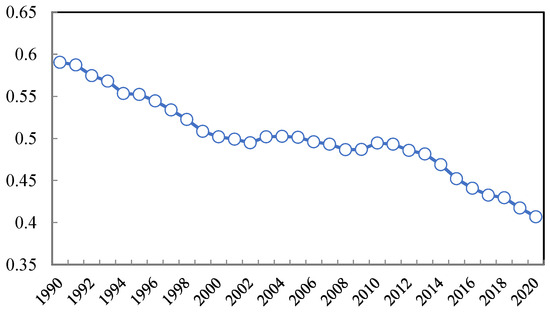
Figure 1.
CO2 emissions (kg per USD 2015 of GDP), 1990–2020.
In years of decreasing carbon dioxide emissions, the number of intergovernmental organizations is increasing. The term intergovernmental organization (IGO) refers to an entity created by treaty, involving two or more nations, to work in good faith on issues of common interest. An intergovernmental organization is not a country but exists independently of sovereign states. The European coordination mechanism of the Quadruple Alliance signed by Britain, Austria, Russia, and Prussia in 1814 directly promoted the emergence of international organizations, namely the Central Commission for the Navigation of the Rhine. The Central Commission for the Navigation of the Rhine, established in 1816, marked the birth of intergovernmental organizations.
Figure 2 shows the number of different intergovernmental organizations from 1909 to 2013. We collect the data from past editions of the Yearbook of International Organizations released by the Union of International Associations (UIA). We can see that conventional international bodies of IGOs increased rapidly before the 1980s, especially after World War II, while special types of IGO have always been the largest proportion and established faster than other international bodies of IGOs.
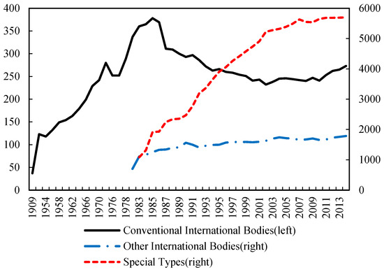
Figure 2.
Historical overview of number of intergovernmental organizations by type 1909–2013 (Appendix A shows the type classification).
Both environmental and non-environmental IGOs play an important role in global climate governance and carbon dioxide emissions. For example, the Food and Agriculture Organization of the United Nations is responsible for paying attention to the protection of natural resources and promoting advanced agricultural production methods. The International Maritime Organization is responsible for protecting the marine environment and the development of the marine environment. The World Health Organization promotes the formulation of standards for drinking water and air quality. The World Bank closely combines environmental protection with financing credit and formulates the policies and procedures for environmental impact assessment as a prerequisite for the World Bank loan project.
After the establishment of many intergovernmental international organizations, environmental protection became one of their goals. Even economic IGOs, such as the World Bank and the International Monetary Fund, have added relevant environmental protection policies and departments. What is the impact of IGOs on global warming? Has national participation in IGOs effectively reduced carbon dioxide emissions? Does the social network relationship generated with other countries in IGOs have an impact on carbon dioxide emissions?
This study aims to investigate whether membership in independent IGOs is truly effective in reducing carbon dioxide emissions, and whether the degree of connectivity among member countries in the IGO network can also effectively reduce carbon dioxide emissions. We use the fixed effect model on global panel data of 168 countries from 1960 to 2014 to estimate the effect of countries joining IGOs on CO2 emissions. We use social network analysis to calculate the degree centrality and closeness centrality of the specific sample country in IGO networks and test the effectiveness on CO2 emissions, respectively. We obtain general conclusions globally through larger databases and more rigorous empirical testing, which has theoretical significance and enriches existing research. We give out policy recommendations for IGOs to encourage countries to reduce CO2 emissions, which has practical significance.
The following content of this study is divided into five parts. The second part constructs a literature review and highlights the originality of this paper by comparing it to other research. The third part consists of the empirical model, variable description, and data. The fourth part carries out the empirical results, including basic results, robustness test, group test, and endogenous test. The fifth part compares the differences between this study and other related studies, discusses the limitations, and concludes the whole paper.
2. Literature Review
A great deal of literature has studied factors that affect the environment, and this section will focus on sorting out the influence and role of international organizations in global environmental protection. International organizations are divided into intergovernmental international organizations (IGOs) and non-governmental international organizations (NGOs). An IGO is a type of alliance or federation of countries, composed of two or more sovereign states, while an NGO is established by private individuals or civil society groups and does not enjoy rights under international law.
The intergovernmental cooperation generated by IGOs is considered an appropriate means of addressing global issues. Most IGOs are established for economic purposes, and safety, health, and the environment are also important goals (Ertrk [1]). World environmental organizations can improve the effectiveness, legitimacy, and efficiency of global environmental governance and should further leverage the role of IGOs in global environmental policy integration and climate security (Dellmuth et al. [2]).
Spilker [3] examined panel data from 114 developing countries from 1970 to 2000 and found that IGOs can provide member countries with resources to obtain the technology needed to reduce pollution and protect the environment, thereby improving the environment of developing countries. Specifically, membership in IGOs can effectively reduce air pollution and greenhouse gas emissions.
Besides Spilker [3], most studies focus on the effect of environmental international organizations. Tosun and Peters [4] found that IGOs focused on Europe and involving the European Commission are more likely to be committed to EPI based on the main legal texts of 78 IGOs. Dellmuth and Gustafsson [5] used quantitative and qualitative data obtained from extensive field surveys from 2017 to 2020 to study the environmental protection practices of IGOs and found that climate change issues that have been incorporated into IGOs are being given more attention.
Many NGOs have played an important role in environmental issues, and with the promotion and support of local citizens and the host country, environmental NGOs can effectively improve the local environmental situation (Pacheco-Vega and Murdie [6]). In addition to directly engaging in environmental protection activities, NGOs can also have a voice and influence in climate negotiations (Gulbrandsen and Andresen [7]).
Longhofer et al. [8] used history event analysis to simulate the transnational situation of environmental policy reforms from 1970 to 2010. The study found that NGOs were closely related to supporting environmental reforms, while the correlation between domestic NGOs and global environmental policies was relatively small. Chiashi [9] used cases of air pollution and industrial pollution in China to study the impact of environmental NGOs on environmental pollution, and found that environmental NGOs are an important force for civil society in solving environmental pollution problems (Aikawa [10]).
Fraser and Temocin [11] sampled 1741 municipalities in Japan and examined the role of environmental NGOs in urban emissions from 2005 to 2017. Their research found that cities with more local NGOs tend to reduce emissions, which strongly supports the efforts of civil society to avoid climate change. Bi et al. [12] identified the disclosure of pollution information by Chinese environmental NGOs as an exogenous shock and found that information disclosure significantly reduced the chemical oxygen demand emissions of manufacturing enterprises.
Li et al. [13] conducted a quantitative analysis based on panel data of environmental non-governmental organizations (ENGOs) and air pollution in OECD countries and found that ENGOs have a positive impact on improving environmental quality, mainly through increasing investment in environmental protection.
By reviewing the literature on the impact of intergovernmental and non-governmental international organizations on environmental protection, we find that there are two limitations in past studies.
First, existing research mostly focuses on case analysis and factual studies, discussing and analyzing through logical inference, lacking quantitative empirical testing. In our study, we use the fixed effect model to carry out empirical tests, and the study contains a series of robustness tests and endogenous tests to ensure the credibility of the results.
Secondly, the research time series of some empirical tests are relatively short and concentrated in specific international organizations or regions, lacking global and greater universality. Therefore, we use a larger global data panel which includes 54 years and 168 countries to find a more general principle.
Thirdly, most literature focuses on studying the impact of environmental international organizations on carbon dioxide emissions, and there is relatively little research on membership in IGOs and the relationships of countries in all IGOs on carbon dioxide reduction. Therefore, we use more credible quantitative tools and the data discussed above to test the following hypothesis.
Hypothesis:
There is a negative relationship between countries joining IGOs and CO2 emissions. The more a specific country joins IGOs, the lower the CO2 emissions produced by that country will be. The more IGOs joined by a specific country that are the same as those joined by other countries and the closer the specific country is to other countries in the IGO network, the lower its CO2 emissions will be.
3. Empirical Model, Variables Description, and Data
We use country panel data to test the impact of countries joining IGOs on CO2 emissions empirically.
3.1. Variable Description and Data
We collect the data of CO2 emissions per capital from 1960 to 2014 given by the World Bank and obtained the smoothing variable lnCO2 as the dependent variable after taking the natural logarithm.
To determine whether an international organization is an IGO, the following three conditions must be met (Wallace and Singer [14]): (1) the intergovernmental organization must be composed of at least three sovereign states; (2) intergovernmental organizations must hold regular plenary meetings at least once every ten years; (3) intergovernmental organizations must have a permanent secretariat and corresponding headquarters.
The Correlates of War Project (COW database) lists the intergovernmental organizations that meet the three conditions mentioned above from 1816 to 2014. We collect the number of IGOs in which the sample countries participated from 1960 to 2014 given by the Correlates of War Project (COW database).
From 1960 to 2014, some countries experienced changes in their political power, resulting in mergers and splits. In order to match countries with databases such as the World Bank, we manually adjusted each regime change country based on its political and economic attributes. The specific adjustment process is as follows.
First, East Germany and West Germany merged in 1990. As East Germany belonged to the Soviet Union and West Germany belonged to the United States, it was not possible to add them together. Therefore, West Germany was assigned to Germany (all literature studying Germany uses West German data as pre-1990 German data).
Second, Czechoslovakia split into two countries, the Czech Republic and Slovakia, after 1993, and the data for Czechoslovakia were directly deleted, while the data for the Czech Republic and Slovakia from 1993 to 2014 were retained.
Third, in 1975, North Vietnam occupied Saigon and South Vietnam was annihilated, resulting in the unification of the north and south into present-day Vietnam. Therefore, North Vietnamese data were retained as Vietnam and South Vietnamese data were deleted as Svietnam.
Fourth, Zanzibar is an integral part of the United Republic of Tanzania with only 2 years of data. Zanzibari data were removed, and Tanzania data were retained.
Fifth, the Republic of Yemen was formed in May 1990 by the merger of the Yemen Arab Republic (North Yemen, Nyemen) and the People’s Democratic Republic of Yemen (South Yemen, Syemen), with Islam as the state religion and Arabic as the official language. Therefore, South Yemen was deleted, and data from North Yemen before 1990 were assigned to the Republic of Yemen.
Sixth, the Republic of Macedonia gained independence from Yugoslavia in 1991. As Yugoslavia was not listed in databases such as the World Bank, Macedonia was retained and Yugoslavia was deleted.
Seventh, East Timor gained independence from Indonesia in 2003 and retained its data unchanged.
Eighth, the original database has already processed data from former Soviet Union countries, so data from countries such as Russia and Ukraine can be directly used.
We assign values to the status of sample countries in IGOs provided in the database. The “Full Membership” status is assigned a value of 1, indicating that in a specific year, the status of a specific sample country in a specific intergovernmental organization was “participating”, while other statuses are assigned a value of 0. We add up the number of IGOs that the sample countries participated in each year and smoothed the natural logarithm to obtain the explanatory variables lnIGO.
IGO networks have similarities with interpersonal networks, and their complexity and the network of connections between individuals also have commonalities. Social network analysis can characterize the clustering effects of different countries in IGOs, which can address endogenous problem. Therefore, we use social network analysis to calculate the degree centrality and closeness centrality of the specific sample country in IGO networks. The degree centrality refers to the number of IGOs jointly participated by the sample country and other countries, revealing the degree of closeness between the sample country and other countries. The closeness centrality is calculated by the distance of the sample country from other countries, which can be used to estimate the time it takes for information or resources to be transmitted.
We use data given by the Correlates of War Project to calculate the degree centrality and closeness centrality of specific sample country, recorded as Degree and Closeness, respectively. We replace the explanatory variable lnIGO with Degree and Closeness in basic regression to ensure the robustness of basic regression.
The following six variables are selected as control variables: natural logarithm of GDP (lnGDP), growth rate of GDP per capita (GDPPg), openness level (Exim), proportion of industrial added value to GDP (Industry), urbanization level (Urban), and proportion of gross capital formation to GDP (Capital). Openness level is calculated by the sum of the proportion of exports and imports of goods and services to GDP. All the control variables are collected from the World Bank. Descriptive statistics of variables are shown in Table 1.

Table 1.
Descriptive statistics of core variables.
In Table 2, we can see that the correlations between independent variables and control variables are not high, with correlation coefficients of less than 0.5., except for two relationships. The correlation between Degree and lnIGO is 0.787 (p < 0.01), and the correlation between Degree and Closeness is 0.814 (p < 0.01). These high correlations result in high VIF values, indicating a potential multicollinearity problem. However, since Degree and lnIGO, as well as Degree and Closeness, do not appear together in the models, there is no multicollinearity issue in practice.
Table 2.
Correlation analysis.
The correlation test between variables is shown in Table 2 to ensure that there is no multicollinearity among the variables before proceeding with the analysis. In Table 2, we can see that the correlations between independent variables and control variables are not high, with correlation coefficients of less than 0.5. Three independent variables are independently entered into the regression equation for fixed effects model testing, and their correlation does not affect the validity of the regression results. In addition, the control variables, except for GDP which is an absolute value, are all relative values. Performing relative value processing on the control variables can effectively reduce the collinearity of macroeconomic variables in time series.
3.2. Empirical Model Selection
This paper studies the impact of countries joining IGOs on air pollution by choosing CO2 emissions as the dependent variable and choosing the number of IGOs participated in as the independent variable. We want to focus on the coefficient β1 of the core independent variable (lnIGO) to see whether there is a significantly negative relationship between CO2 emissions and the act of joining IGOs. The model is constructed as the following Equation (1).
where i represents the ith country and t represents the tth year. lnCO2 is the dependent variable, and lnIGO is the explanatory variable. X represents the control variables, including natural logarithm of GDP (lnGDP), growth rate of GDP per capita (GDPPg), openness level (Exim), proportion of industrial added value to GDP (Industry), urbanization level (Urban), and proportion of gross capital formation to GDP (Capital).
In light of the differences among different countries, we first construct the panel variable coefficient model and select the optimal model based on the model estimation results. In addition, individual fixed effects or individual random effects need to be chosen when constructing the model. The fixed effect model is shown as Equation (2), followed by Zhang et al. [15], where Countryi captures the country fixed effect, and yeart captures the year fixed effect.
The random effect model is shown as Equations (3) and (4).
To decide which model is much more appropriate to conduct, we use the Hausman test. The null hypothesis behind the Hausman test is that there is no significant difference in the estimators between the fixed effects model and the random effects model. If the null hypothesis is rejected, the conclusion is that the random effects model is not appropriate, because the random effects may be related to one or more regressors. In this case, the fixed effects model is better than the random effects model. The results of the Hausman test are shown in Table 3. According to the Hausmann test (Prob < 0.10), we should build a model of fixed effects.
Table 3.
The results of the Hausman test.
As for country panel data, there may be cross-section dependence and slope heterogeneity in the sample. It is better to test cross-section dependence and slope heterogeneity before choosing the final regression model. If the panel data has the property of cross-section dependence and slope heterogeneity, common correlated effects mean group (CCEMG) estimator and the augmented mean group (AMG) estimator need to be applied. However, the sample data in this study are too unbalanced to conduct the two tests mentioned above, and the square terms in the model are not well applied to the tests. Therefore, we still choose the fixed effects model, which can meet the needs of the short unbalanced data and square terms followed by Li et al. [16]. In addition, to solve the problem of heteroscedasticity and sequence autocorrelation in the panel data, the fixed effects regression is clustered to the country and year level, followed by Azzimonti [17].
4. Estimated Results and Discussion
4.1. Basic Regression Results
The basic fixed effects regression results of Equation (2) are shown in Table 4. Columns (1) and (2) of Table 4 use the number of IGOs in which the specific countries participated as core independent variables. We do not control any variables in column (1). The empirical result of column (1) shows that the coefficient of lnIGO is −0.3, which is significant at the 1% level. This indicates that there is a negative relationship between CO2 emissions and countries joining IGOs and that joining IGOs can reduce CO2 emissions effectively. The larger the number of IGOs the specific sample country joins, the lower the CO2 emissions produced by the country will be. This is consistent with the hypothesis.
Table 4.
Basic Result.
We add all control variables in column (2). The number of observations drops from 4509 to 3570, and the number of sample countries drops from 187 to 168, as some countries are missing the control variables (the same data availability problem exists in Table 5, Table 6 and Table 7). From column (2), we can find that the coefficient of lnIGO is still negative, the value (−0.266) is stable, and it is significant at the 1% level, which means joining IGOs can still reduce CO2 emissions effectively after controlling other factors affecting CO2 emissions.
Table 5.
Robustness test.
Table 6.
Group test.
Table 7.
Endogenous test.
In column (1), we can find that CO2 emissions will decrease by 0.3 percentage points for each additional IGO joined by a sample country. In column (2), we can find that CO2 emissions will decrease by 0.266 percentage points for each additional IGO joined by a sample country. The regression coefficients of the control variables in column (2) indicate that increases in GDP scale and growth rate of GDP per capita will reduce CO2 emissions, while increases in industry level, urbanization, and capital accumulation will increase CO2 emissions.
Obtaining membership in IGOs takes some time, and it is not an immediate group to join. The more memberships a country has in IGOs, the more connections it has with other countries, whether economic, political, or social. The connections of countries in these international organizations will reduce carbon dioxide emissions through various channels.
We replace IGO numbers (lnIGO) with the distance of the sample country from other countries in IGO networks (Closeness) in column (3) and column (4). The empirical result of column (3) shows that the coefficient of Closeness is −9.869, which is significant at the 1% level. The empirical result of column (4) controls all other facts and shows that the coefficient of Closeness is −6.442, which is still significant at the 1% level. This implies that the relationship of CO2 emissions will be effectively reduced if the distance of the sample country from other countries in IGO networks is less.
In column (4), we can find that CO2 emissions will decrease by 6.442 percentage points for every 1% closer the sample country is to other countries in IGO networks. The regression coefficients of the control variables in column (4) also indicate that the increase of GDP scale and growth rate of GDP per capita will reduce CO2 emissions, while the increase of industry level, urbanization and capital accumulation will increase CO2 emissions, which are all significant. The coefficients of control variables remain stable, which implies the robustness of the regression model.
We replace IGO numbers (lnIGO) with the number of IGOs jointly participated by the sample country and other countries (Degree) in column (5) and column (6). The empirical result of column (5) shows that the coefficient of Degree is −3.609, which is significant at the 1% level. The empirical result of column (6) controls all other facts and shows that the coefficient of Degree is −2.271, which is still significant at the 10% level. We can see that the more IGOs jointly participated in by the sample country and other countries, the lower CO2 emissions will be.
In column (6), we can find that CO2 emissions will decrease by 2.271 percentage points for every additional same IGO joined by the sample country and other countries. The regression coefficients of the control variables in column (6) also indicate that increases in GDP scale and growth rate of GDP per capita will reduce CO2 emissions, while increases in industry level, urbanization, and capital accumulation will increase CO2 emissions, which are all significant. The coefficients of control variables remain stable, which implies the robustness of the regression model.
4.2. Robustness Test and Group Test
Although column (3) to column (6) in Table 4 shows the robustness of the basic conclusion, we still need to carry out the robustness test shown to ensure the reliability of all basic regression results. We cut the timeline of database starting from 1990 to 2014, as significant changes occurred in the world political and economic landscape after the 1990s with the dissolution of the Soviet Union. The result of the robustness test is shown in Table 5.
In column (1) and column (2) of Table 5, we use the total IGO numbers (lnIGO) joined by the sample countries as the independent variable. Column (1) does not include control variables, while column (2) includes all control variables. The results show that the coefficients of lnIGO are negative in both columns, indicating there is a negative relationship between CO2 emissions and IGO numbers joined by the sample countries, which is consistent with the basic regression results. The coefficients of the control variables in column (2) are also consistent with the basic regression results. We can also find that the absolute values of coefficients of lnIGO in column (1) and column (2) in Table 5 are a little bit larger than those in Table 4. After the 1990s, the effectiveness of reducing CO2 emissions becomes better if the sample country joins more IGOs.
In column (3) and column (4) of Table 5, we use the distance of the sample country from other countries in IGO networks (Closeness) as the independent variable. Column (3) does not include control variables, while column (4) includes all control variables. The results show that the coefficients of Closeness are negative in both columns, indicating there is a negative relationship between CO2 emissions and the distance of the sample country from other countries in IGO networks, which is consistent with the basic regression results. The coefficients of control variables in column (4) are also consistent with the basic regression results. We also find that the absolute values of the coefficients of Closeness in column (3) and column (4) in Table 5 are also larger than that in Table 4. After the 1990s, the effectiveness of reducing CO2 emissions becomes better if the distance of countries in IGO networks becomes less.
In column (5) and column (6) of Table 5, we use the number of IGOs jointly participated in by the sample country and other countries (Degree) as the independent variable. Column (5) does not include control variables, while column (6) includes all control variables. The results show that the coefficients of Degree are negative in both columns, indicating there is a negative relationship between CO2 emissions and the number of same IGOs joined by the sample country and other countries, which is consistent with the basic regression results. The coefficients of control variables in column (6) are also consistent with the basic regression results. We also find that the absolute values of coefficients of Degree in column (5) and column (6) in Table 5 are also larger than that in Table 4. After the 1990s, the effectiveness of reducing CO2 emissions becomes better if sample countries participate in more of the same IGOs as other countries.
For further analysis, we divide IGOs into three different types collected from the COW project: political IGOs (lnigo_political), social IGOs (lnigo_social), and economic IGOs (lnigo_economic). We want to test the impact of the number of sample countries participating in different IGOs on carbon dioxide emissions. The group regression results are shown in Table 6. We can find that all the coefficients are negative and the absolute values of all the coefficients are smaller than those in column (1) and column (2) of Table 4. We can find that the absolute values of the coefficients are larger in column (3) and column (4) than other columns, which implies that joining more social IGOs can reduce more CO2 emissions than joining political and economic IGOs. This makes sense because environmental IGOs are classified as social IGOs. It is worth noting that the regression coefficients in all columns are significant except those in column (4).
We can find that CO2 emissions will decrease by 0.174 percentage points for each additional political IGO joined by a sample country from column (2) and will decrease by 0.201 percentage points for every additional political IGO joined by a sample country from column (6). The regression coefficients of the control variables in column (2), column (4), and column (6) are stable and consistent with prior results.
4.3. Endogenous Problem
We apply the instrumental variables (IV)–two-stage least-squares (2SLS) method to avoid the endogenous problem caused by reciprocal causation between CO2 emissions and IGOs joined by the sample countries. The results of the endogenous test are shown in Table 7. We use the first-order lag term of independent variables as an instrumental variable to check the reliability of the basic results in column (1) and column (2), following Song et al. [18], and use the Durbin–Wu-Hausman test (DWH Test) to check whether the independent variables are endogenous or not. If the p-value of the DWH Test is smaller than 0.05 or 5%, then the variable is endogenous.
From Table 7, we can find that the endogenous problem of independent variables exists in all columns except column (4), which implies that there is an endogenous problem both statistically and logically in economics. Therefore, we use the instrumental variables (IV)–two-stage least-squares (2SLS) method to solve it.
The regression coefficients from column (1) to column (6) are consistent with the basic regression results. We can find that joining more IGOs can effectively reduce more CO2 emissions from column (1) and column (2). We can also find that CO2 emissions will be reduced more if the distance of countries in IGO networks becomes less and if countries join more of the same IGOs. After using the instrumental variables (IV)–two-stage least-squares (2SLS) method to avoid endogenous problem, the regression results are still significant at the 1% level. Therefore, we come to conclusion that the proposition can be proved and the negative relationship between CO2 emissions and joining IGOs by sample countries is reliable and credible.
4.4. Caveats
Although we carried out the endogenous test above to control for the reciprocal causation between CO2 emissions and IGOs, the dually endogenous nature of IGO membership and carbon emissions still exists. Even though the conclusions of this study are still significant after endogeneity testing in statistics, there may still be endogeneity issues in economic logic and reality.
For example, the establishment goal of the European Union (EU) is an economic and geopolitical block and the creation of the Eurozone is as a monetary union. It stands to reason that countries did not join such organizations or bankroll such projects for whimsical reasons. They did so with the intent of bolstering regional economic integration, consolidating geopolitical power, promoting international trade, capital flows, and human capital allocation, among other factors. Critically, when countries have such economic and geopolitical objectives, it is not by coincidence that they also abide by higher standards of international governance, which may include carbon emission reductions—an effect that likely became even stronger due to the increasing relevance of ESG investors.
There are a few examples of how the Eurozone membership may facilitate carbon emission reductions. Dantas et al. [19] show a monetary union provides its banks and non-financial companies with stronger government guarantees. Stronger guarantees bolster credit to projects related to green innovation, thereby reducing carbon emissions. Cortes et al. [20] show a monetary union and establishment of the ECB as a lender of last resort also facilitates monetary policy coordination and is essential to reducing disaster risks in periods of distress. The two examples above are in the context of European jurisdictions, but the economics apply to any country joining IGO, which are likely accompanied by reductions in emissions, and it is unclear which one comes first: the economic benefits of IGO membership or better governance due to the intent of joining IGOs.
5. Discussion and Conclusions
Since the Industrial Revolution, emissions of greenhouse gases such as CO2 have soared in various countries. After the establishment of many intergovernmental international organizations, environmental protection has become one of their goals. Even economic IGOs, such as the World Bank and the International Monetary Fund, have added relevant environmental protection policies and departments. What is the impact of IGOs on global warming? Has national participation in IGOs effectively reduced carbon dioxide emissions? Does the social network relationship generated with other countries in IGOs have an impact on carbon dioxide emissions? This paper studies the impact of IGO membership on CO2 emissions.
5.1. Discussion and Limitation
There are some limitations of this studies which need to be addressed in further research. Firstly, the data used in this study are from 1960 to 2014. If available in the future, the time series will need to be extended and the data will be updated to 2024 for further research. Secondly, this article studied the effects of IGO membership and closeness in IGO networks on carbon dioxide emissions but did not investigate their mechanisms of action. Detailed research and testing are needed in the future. Finally, in social network analysis, this study assigned equal weight to membership in different IGOs, but some IGOs have greater discourse power than others in the real world. In future research, it will be necessary to quantitatively measure the weight of IGOs and observe in more detail the impact of adding different types of IGOs on carbon dioxide emissions.
5.2. Conclusions
This paper uses global panel data from 168 countries from 1960 to 2014 to carry out the fixed effect regression. The results of basic regression show that there is a negative relationship between CO2 emissions and countries joining IGOs. The greater the number of IGOs the specific sample country joins, the lower the CO2 emissions produced by the country will be. This finding aligns with international environmental agreements like the Paris Agreement. By the end of 2024, more than 130 countries had announced their goal of achieving net zero emissions by the mid-21st century. When there are more intergovernmental international organizations in which a country participates, the goal of reducing carbon dioxide emissions will be easier to achieve.
We also use social network analysis and find that the relationship of CO2 emissions will be effectively reduced if the distances of the sample country from other countries in IGO networks are smaller. The more IGOs jointly participated in by the sample country and other countries, the lower CO2 emissions will be. Joining more social IGOs can reduce more CO2 emissions than joining political and economic IGOs.
This study is a supplement to previous research and provides reliable data validation and conclusion support. We have obtained general conclusions globally through larger databases and more rigorous empirical testing, which has theoretical significance. We give out policy recommendations for IGOs promoting countries to reduce CO2 emissions, which has practical significance.
5.3. Implication
According to the results of this study, we give out the following policy implications. In the current stage, the existence of IGOs is essential for global environmental protection and the governance of climate change. IGOs provide a good platform for consultation, communication, and rule-making in environmental governance among countries. Countries should be encouraged to actively participate in IGOs according to the following recommendations. First, add more environmental targets in addition to economic objectives in economic IGOs. When a country wants to obtain economic benefits in economic IGOs, it should also comply with the rules for reducing carbon dioxide emissions. Secondly, cooperation should be established between different types of IGOs. For example, climate conferences can be jointly organized by different types of IGOs, and the goal of reducing carbon dioxide often requires cooperation from different social sectors in various countries to achieve.
Author Contributions
This study is the result of teamwork. T.H. and X.L. equally contributed in designing the study, analyzing the data, writing the draft, and revising the study. Authors are ranked alphabetically by author’s last name. All authors have read and agreed to the published version of the manuscript.
Funding
This research received no external funding.
Institutional Review Board Statement
Not applicable.
Informed Consent Statement
Not applicable.
Data Availability Statement
Data are contained within the article.
Conflicts of Interest
The authors declare no conflict of interest.
Appendix A. Union of International Organizations Classification Standards
| Type | Group | Name | Examples |
| Conventional International Bodies | A | Federations of international organizations | United Nations, International Disability Alliance |
| B | Universal membership organizations | International Alliance of Women, International Council of Museums | |
| C | Intercontinental membership organizations | Adventure Travel Trade Association, World Association for Education Research | |
| D | Regionally oriented membership organizations | European Academy of Sciences, African Boxing Union | |
| Other International Bodies | E | Org’s emanating from places, persons, bodies | Energy Union, Statistical Office of the European Union |
| F | Organizations of special form | Contadora Parliament, Consumer Specialty Products Association | |
| G | Internationally oriented national organizations | Center for Middle East Development, War on Want | |
| Special Types | H | Dissolved or apparently inactive organizations | Committee of European Coffee Associations, Warsaw Treaty Organization |
| J | Recently reported bodies—not yet confirmed | Light Electric Vehicle Association, World Merit | |
| K | Subsidiary and internal bodies | Global Accrediting Group, Global University | |
| N | National organizations | European Police Association, Frontiers Foundation | |
| R | Religious orders and secular institutes | Sisters of Nazareth, Suhrawardiya | |
| S | Autonomous conference series | Asian Composer’s Conference, Economist Conferences | |
| T | Multilateral treaties, intergovernmental agreements | Naval Agreement, Nyon Arrangement | |
| U | Currently inactive nonconventional bodies | Computer People for Peace, Confederation of Chivalry |
References
- Ertrk, E. Intergovernmental Organizations (IGOs) and Their Roles and Activities in Security, Economy, Health and Environment. J. Int. Soc. Res. 2015, 8, 333. [Google Scholar] [CrossRef]
- Dellmuth, L.M.; Gustafsson, M.T.; Bremberg, N.; Mobjörk, M. Intergovernmental Organizations and Climate Security: Advancing the Research Agenda. Wiley Interdiscip. Rev. Clim. Change 2018, 9, e496. [Google Scholar] [CrossRef]
- Spilker, G. Helpful Organizations: Membership in Intergovernmental Organizations and Environmental Quality in Developing Countries. Br. J. Political Sci. 2016, 42, 345–370. [Google Scholar] [CrossRef]
- Tosun, J.; Peters, B.G. Intergovernmental Organizations’ Normative Commitments to Policy Integration: The Dominance of Environmental Goals. Environ. Sci. Policy 2018, 82, 90–99. [Google Scholar] [CrossRef]
- Dellmuth, L.M.; Gustafsson, M.T. Global Adaptation Governance: How Intergovernmental Organizations Mainstream Climate Change Adaptation. Clim. Policy 2021, 21, 868–883. [Google Scholar] [CrossRef]
- Pacheco-Vega, R.; Murdie, A. When do Environmental NGOs Work? A Test of the Conditional Effectiveness of Environmental Advocacy. Environ. Polit. 2020, 2, 1–22. [Google Scholar] [CrossRef]
- Gulbrandsen, L.H.; Andresen, S. NGO Influence in the Implementation of the Kyoto Protocol: Compliance, Flexibility Mechanisms, and Sinks. Glob. Environ. Politics 2004, 4, 54–75. [Google Scholar] [CrossRef]
- Longhofer, W.; Schofer, E.; Miric, N. NGOs, INGOs, and Environmental Policy Reform, 1970–2010. Soc. Forces 2016, 94, 1743–1768. [Google Scholar] [CrossRef]
- Chiashi, A. Multi-tiered Nature of Environmental Pollution Problems and the Pollution Control Governance in China: The Role of Environmental NGOs. Environ. Policy Gov. China 2017, 25, 159–176. [Google Scholar] [CrossRef]
- Aikawa, Y. Environmental NGOs and Environmental Pollution in China. Environ. Policy Gov. China 2017, 25, 177–194. [Google Scholar] [CrossRef]
- Fraser, T.; Temocin, P. Grassroots vs. Greenhouse: The Role of Environmental Organizations in Reducing Carbon Emissions. Clim. Change 2021, 169, 1–22. [Google Scholar] [CrossRef]
- Bi, R.; Kou, Z.; Zhao, C. Information Disclosure and Pollution Reduction: Evidence from Environmental NGO Monitoring in China. Econ. Anal. Policy 2024, 82, 1459–1473. [Google Scholar] [CrossRef]
- Li, G.; He, Q.; Wang, D. Environmental Non-governmental Organizations and Air-pollution Governance: Empirical Evidence from OECD Countries. PLoS ONE 2021, 16, 1–17. [Google Scholar] [CrossRef] [PubMed]
- Wallace, M.; Singer, J. International Governmental Organization in the Global System, 1815–1964: A Quantitative Description. Int. Organ. 1970, 24, 239–287. [Google Scholar] [CrossRef]
- Zhang, N.; Yu, K.; Chen, Z. How does Urbanization Affect Carbon Dioxide Emissions? A Cross-Country Panel Data Analysis. Energy Policy 2017, 107, 678–687. [Google Scholar] [CrossRef]
- Li, X.Y.; Liu, J.; Ni, P. The Impact of Digital Economy on CO2 Emissions: A Theoretical and Empirical Analysis. Sustainability 2021, 13, 7267. [Google Scholar] [CrossRef]
- Azzimonti, M. Does Partisan Conflict Deter FDI Inflows to the US? J. Int. Econ. 2019, 120, 162–178. [Google Scholar] [CrossRef]
- Song, Y.; Hao, F.; Hao, X.; Gozgor, G. Economic Policy Uncertainty, Outward Foreign Direct Investments, and Green Total Factor Productivity: Evidence from Firm-level Data in China. Sustainability 2021, 13, 2339. [Google Scholar] [CrossRef]
- Dantas, M.; Merkley, K.J.; Silva, F.B.G. Government Guarantees and Banks’ Income Smoothing. J. Financ. Serv. Res. 2023, 6, 123–173. [Google Scholar] [CrossRef]
- Cortes, G.S.; Gao, G.P.; Silva, F.B.G. Unconventional Monetary Policy and Disaster Risk: Evidence from the Subprime and COVID-19 Crises. J. Int. Money. Financ. 2022, 122, 102543. [Google Scholar] [CrossRef] [PubMed]
Disclaimer/Publisher’s Note: The statements, opinions and data contained in all publications are solely those of the individual author(s) and contributor(s) and not of MDPI and/or the editor(s). MDPI and/or the editor(s) disclaim responsibility for any injury to people or property resulting from any ideas, methods, instructions or products referred to in the content. |
© 2025 by the authors. Licensee MDPI, Basel, Switzerland. This article is an open access article distributed under the terms and conditions of the Creative Commons Attribution (CC BY) license (https://creativecommons.org/licenses/by/4.0/).