Energy–Carbon Coupling Modeling of Integrated Energy Systems in Low-Carbon Parks

Abstract

In integrated energy system modeling, extant research predominantly addresses single-energy system optimization or carbon emission flow models, failing to adequately elucidate the mechanisms of combined energy and carbon flow modeling in complex energy systems. This deficiency hampers a thorough analysis of the coupling relationships between energy and carbon flows, thereby posing significant challenges for resource allocation and carbon mitigation within integrated energy systems. This paper presents an innovative energy–carbon coupling model, constructing a unified framework for energy and carbon flow modeling centered on the energy hub, thereby overcoming the limitations of traditional approaches that are unable to model both energy and carbon flows concurrently. The model comprehensively examines the coupling nodes and carbon density correlations among energy conversion devices within multi-energy systems, precisely quantifying carbon emission paths and distribution across devices. This provides a novel methodology for carbon emission management in integrated energy systems. Case studies on typical integrated energy systems demonstrate the proposed model’s efficacy in low-carbon economic dispatch. The energy–carbon coupling model developed in this study offers a high-adaptability solution for integrated energy systems in multi-energy, low-carbon parks, achieving an optimal balance between economic efficiency and environmental performance under dual objectives of energy demand and carbon emission minimization.

1. Introduction

With increasing global attention on climate change, nations worldwide have set ambitious carbon neutrality targets aimed at addressing the challenges posed by climate change through carbon emission control. China has likewise pledged to achieve carbon neutrality by 2060 [1]. Against this backdrop, the development of smart low-carbon parks has emerged as an essential path for promoting energy system transformation, enhancing energy efficiency, and reducing carbon emissions. Consequently, low-carbon, energy-efficient, and clean integrated energy systems (IESs) have become a significant research focus in the field of power systems in recent years. An IES is defined as an energy configuration that, centered around the power system, couples multiple energy subsystems—such as heating, cooling, and natural gas—while coordinating and optimizing each phase of “source-network-load-storage” from a physical perspective during the planning, construction, and operational stages, resulting in an integrated system of energy production, supply, and utilization [2]. Modeling and optimizing the energy and carbon flows within an IES can increase energy utilization efficiency, reduce carbon emissions [3], and facilitate multi-energy complementarity and large-scale renewable energy deployment. This not only provides technical support for achieving the “zero-carbon” goal in energy systems but also lays a solid foundation for the promotion and application of smart low-carbon parks in the future [4].

Research on IES modeling has made considerable progress. Literature [5] proposes an energy hub model concept that succinctly illustrates the coordination and coupling relationships among multiple energy flow conversion units within the system, including electricity, gas, heat, and renewable energy. Literature [6] develops a multi-objective optimization model for the operation and planning of building-level energy stations based on energy hubs, optimizing cooling, heating, and electrical outputs. Literature [7] considers scenarios in which multi-energy flow systems comprise multiple energy hubs, using the principles of non-cooperative game theory to establish a corresponding model based on the interdependencies of coupling, complementarity, and constraints among hubs. This model yields optimized scheduling results at various confidence levels and analyzes their impacts. Literature [8] presents a novel carbon emission flow analysis model for multi-energy systems to quantify carbon emissions associated with energy transfer and conversion processes, validated through case studies. Research on low-carbon economic optimization dispatch for IESs varies by the factors considered, leading to different optimization approaches. Literature [9] develops an economic optimization dispatch model that aims to minimize the life-cycle costs of IES construction and operation within a park. The study demonstrates that the coupling and scheduling of subsystems can flexibly integrate multiple energy conversion devices, significantly reducing dependence on external energy purchases and overall system costs. Literature [10] addresses the uncertainty of supply and demand within the energy system, proposing a two-stage modeling and multi-energy flow solution method that enhances economic efficiency while reducing carbon emissions through the coordinated control of various resources. Literature [11] introduces a bilevel optimization model for low-carbon economic dispatch by accurately accounting for implied carbon emissions through the carbon flow density of external electricity sources, effectively optimizing the carbon flow distribution within the IES and enhancing system environmental performance. Literature [12] presents a coordinated optimization approach that considers long- and short-term hydrogen storage, demand response, and multiple uncertainties. The results indicate that the proposed optimization approach reduces system costs, minimizes energy waste, and achieves zero emissions.

Modeling energy and carbon flows within an IES is a complex yet critical task, providing the foundation for integrated energy–carbon optimization in smart low-carbon parks. The studies mentioned above, based on energy hub theory, model either energy or carbon flows within an IES and apply various optimization targets to optimize system dispatch. However, significant challenges persist in constructing a combined energy–carbon flow model: First, IESs typically incorporate multiple forms of energy with intricate conversion and coupling relationships, necessitating the consideration of different energy conversion pathways and the interdependence between energy and carbon flows during modeling, which significantly increases model complexity. Second, current modeling approaches face difficulties in achieving an integrated modeling of energy and carbon flows, failing to effectively reflect the coupling relationship between energy and carbon emissions within the system.

To address the complexities and challenges associated with modeling energy and carbon flows within IES, energy hub theory offers a new perspective and solution. First, energy hubs effectively integrate various forms of energy, simplifying conversion pathways among different energy types, which clarifies complex coupling relationships during the modeling process. This integrated framework enables simultaneous consideration of the interdependence between energy and carbon flows within a unified model, more accurately reflecting the coupling between energy and carbon emissions within the system. Moreover, a significant challenge of energy–carbon-coupled modeling in this study lies in balancing model accuracy with computational complexity reduction. The assumptions made during the modeling process tend to be idealized, excluding factors such as equipment aging and failures. Under ideal conditions, the model assumes adjustable equipment efficiency and high operational stability of the system environment.

To address these issues, this paper proposes an innovative energy–carbon coupling model based on the energy hub framework. This model offers the ability to couple and integrate multiple energy types, effectively managing the conversion and flow of various energy forms. The energy–carbon coupling model not only accurately represents energy conversion processes but also embeds carbon emission factors, enabling a precise calculation of carbon emissions at each step of energy conversion. This clear representation of the coupling between energy and carbon flows enables an integrated modeling of both flows. Additionally, the model can calculate carbon emissions across the four major components of an IES—source, network, load, and storage—supporting life-cycle carbon emission management. By combining energy and carbon flow models, the energy–carbon coupling model simplifies the separate modeling process, reduces computational complexity, and clarifies and unifies the representation and calculation of energy and carbon flows.

The main contributions of this study can be summarized as follows:

• This study proposes an energy hub-based energy–carbon coupling modeling method, achieving a simultaneous integrated modeling of multiple energy flows and carbon flows and effectively revealing the complex coupling between energy conversion and carbon emissions within the system.
• By analyzing carbon emissions across the four major components of an IES—source, network, load, and storage—the study realizes life-cycle carbon emission management, enhancing system efficiency, supporting national carbon reduction goals, and providing solid technical support for the promotion of smart low-carbon parks.
• By simplifying the computational process for complex energy and carbon flow coupling, the model significantly reduces computational complexity while ensuring accuracy, thereby enhancing the efficiency and operability of optimized dispatch, making the model more feasible for practical engineering applications.

2. Construction of the Coupled Energy and Carbon Flow Model for Integrated Energy Systems

The integrated energy system is generally dominated by electricity and natural gas, with the energy supply network composed of power distribution networks, thermal pipelines, cooling supply networks, and natural gas pipelines. The system includes various energy conversion and storage devices to meet the demands for four types of loads—electricity, heat, cooling, and gas—on the user side. The energy conversion devices primarily consist of photovoltaic (PV) systems, wind turbines (WTs), gas turbines (EGTs), gas boilers (GHBs), electric boilers (EHBs), electric chillers (ECs), absorption chillers (ACs), carbon capture and storage (CCS) units, power-to-gas (P2G) systems, and combined cooling, heating, and power (CCHP) units. The energy storage devices include energy storage batteries (ES), thermal storage tanks (HS), chilled storage tanks (CS), and gas storage tanks (GS). A specific structural diagram of the integrated energy system is shown in Figure 1. This paper constructs the models of various energy conversion devices based on ideal operating conditions, assuming stable device performance with fixed parameters, and does not consider the impact of device aging or environmental changes on the energy conversion efficiency.

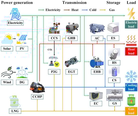
Figure 1. Specific structure of the integrated energy system.

2.1. Models of Various Devices in the Integrated Energy System

2.1.1. Gas Turbine

The gas turbine (EGT) operates under optimal conditions, where the power consumed by the combustion of natural gas and the power generated can be expressed as follows:

$$P_{\mathrm{EGT}}{\eta }_{\mathrm{EGT},\mathrm{e}}=P_{\mathrm{EGT},\mathrm{e}}$$

(1)

The relationship between the carbon flow density at the input and output ports of the gas turbine can be expressed as follows:

$${\rho }_{\mathrm{EGT}}{\eta }_{\mathrm{EGT},\mathrm{e}}={\rho }_{\mathrm{EGT},\mathrm{e}}$$

(2)

where $P_{\mathrm{EGT}}$ represents the gas consumption power of the gas turbine, $P_{\mathrm{EGT},\mathrm{e}}$ is the power generated by the gas turbine, ${\rho }_{\mathrm{EGT}}$ denotes the carbon flow density at the input port of the gas turbine, ${\rho }_{\mathrm{EGT},\mathrm{e}}$ is the carbon flow density at the output port for the electric load of the gas turbine, and ${\eta }_{\mathrm{EGT},\mathrm{e}}$ represents the power generation efficiency of the gas turbine.

2.1.2. Gas Boiler

Under suitable operating conditions, the gas boiler (GHB) consumes natural gas and converts the internal energy of the gas into thermal energy. The specific energy conversion relationship is as follows:

$$P_{\mathrm{GHB}}{\eta }_{\mathrm{GHB}}=P_{\mathrm{GHB},\mathrm{h}}$$

(3)

The relationship between the carbon flow density at the input and output ports of the gas boiler can be expressed as follows:

$${\rho }_{\mathrm{GHB}}{\eta }_{\mathrm{GHB}}={\rho }_{\mathrm{GHB},\mathrm{h}}$$

(4)

where $P_{\mathrm{GHB}}$ represents the gas consumption power of the gas boiler, $P_{\mathrm{GHB},\mathrm{h}}$ denotes the heat output power of the gas boiler, ${\rho }_{\mathrm{GHB}}$ is the carbon flow density at the input port of the gas boiler, ${\rho }_{\mathrm{GHB},\mathrm{h}}$ is the carbon flow density at the output port of the gas boiler, and ${\eta }_{\mathrm{GHB}}$ signifies the energy conversion efficiency of the gas boiler.

2.1.3. Electric Boiler

The electric boiler (EHB) directly converts electrical energy into thermal energy to supply the user load. Under suitable operating conditions, the energy conversion relationship can be expressed as follows:

$$P_{\mathrm{EHB}}{\eta }_{\mathrm{EHB}}=P_{\mathrm{EHB},\mathrm{h}}$$

(5)

The relationship between the carbon flow density at the input and output ports of the electric boiler can be expressed as:

$${\rho }_{\mathrm{EHB}}{\eta }_{\mathrm{EHB}}={\rho }_{\mathrm{EHB},\mathrm{h}}$$

(6)

where $P_{\mathrm{EHB}}$ represents the power consumption of the electric boiler, $P_{\mathrm{EHB},\mathrm{h}}$ denotes the heat generation power of the electric boiler, ${\rho }_{\mathrm{EHB}}$ indicates the carbon flow density at the input port of the electric boiler, ${\rho }_{\mathrm{EHB},\mathrm{h}}$ signifies the carbon flow density at the output port of the electric boiler, and ${\eta }_{\mathrm{EHB}}$ represents the energy efficiency of the electric boiler.

2.1.4. Electric Chiller

The electric chiller (EC) operates by consuming electrical energy for cooling. Under suitable operating conditions, its operational model is similar to that of a lithium bromide absorption chiller:

$$P_{\mathrm{EC}}{\eta }_{\mathrm{EC}}=P_{\mathrm{EC},\mathrm{c}}$$

(7)

The relationship of carbon flow density at the input and output ports of the electric chiller can be expressed as follows:

$${\rho }_{\mathrm{EC}}{\eta }_{\mathrm{EC}}={\rho }_{\mathrm{EC},\mathrm{c}}$$

(8)

In the equation, $P_{\mathrm{EC}}$ and $P_{\mathrm{EC},\mathrm{c}}$ represent the power consumption and cooling power of the electric chiller, respectively; ${\rho }_{\mathrm{EC}}$ and ${\rho }_{\mathrm{EC},\mathrm{c}}$ denote the carbon flow density at the input and output ports of the electric chiller, respectively; and ${\eta }_{\mathrm{EC}}$ signifies the coefficient of the performance of the electric chiller.

2.1.5. Absorption Chiller

The absorption chiller (AC) operates under suitable conditions, converting thermal energy into cooling energy to directly meet the cooling demands of users. Let the input thermal power of the absorption chiller be denoted as $P_{\mathrm{AC}}$ and the output cooling power as $P_{\mathrm{AC},\mathrm{c}}$. The relationship between them can be expressed as follows:

$$P_{\mathrm{AC}}{\eta }_{\mathrm{AC}}=P_{\mathrm{AC},\mathrm{c}}$$

(9)

The carbon flow density relationship between the input and output ports of the absorption chiller can be expressed as follows:

$${\rho }_{\mathrm{AC}}{\eta }_{\mathrm{AC}}={\rho }_{\mathrm{AC},\mathrm{c}}$$

(10)

In the equation, ${\eta }_{\mathrm{AC}}$ represents the coefficient of performance of the absorption chiller, commonly referred to as the energy efficiency ratio, which indicates the ratio of the cooling capacity to the heat input of the absorption chiller during operation. ${\rho }_{\mathrm{AC}}$ and ${\rho }_{\mathrm{AC},\mathrm{c}}$ represent the carbon flow densities at the input and output ports of the absorption chiller, respectively.

2.1.6. Carbon Capture System

The carbon capture system (CCS) solely consumes electrical energy to enrich CO₂, which is then transported to the power-to-gas (P2G) system. Within the integrated energy system, CCS serves as a consumer of electrical energy and does not generate any cooling, heating, electrical, or gas loads. The energy hub model for CCS is characterized by one input and zero outputs. The quantity corresponding to the input end of the coupling matrix is denoted by 1, indicating that all the electrical energy input to the CCS system is utilized.

2.1.7. Power-to-Gas

The power-to-gas (P2G) system operates under suitable conditions, where the power consumed for the electrolysis of water and the hydrogen production power can be expressed as follows:

$$P_{\mathrm{P}2\mathrm{G}}{\eta }_{\mathrm{P}2\mathrm{G}}=P_{\mathrm{P}2\mathrm{G},\mathrm{g}}$$

(11)

The relationship between the carbon flow density at the input and output ports of the P2G can be expressed as follows:

$${\rho }_{\mathrm{P}2\mathrm{G}}{\eta }_{\mathrm{P}2\mathrm{G}}={\rho }_{\mathrm{P}2\mathrm{G},\mathrm{g}}$$

(12)

where $P_{\mathrm{P}2\mathrm{G}}$ represents the power consumed by the electrolysis of water, $P_{\mathrm{P}2\mathrm{G},\mathrm{g}}$ denotes the hydrogen production power of the P2G system, ${\rho }_{\mathrm{P}2\mathrm{G}}$ is the carbon flow density at the input port of the P2G, ${\rho }_{\mathrm{P}2\mathrm{G},\mathrm{g}}$ is the carbon flow density at the output port of the P2G, and ${\eta }_{\mathrm{P}2\mathrm{G}}$ represents the energy conversion efficiency of the P2G system.

2.1.8. Combined Cooling, Heating, and Power System

The relationships among the power consumed by the combustion of natural gas, the power generated, the thermal power produced, and the cooling power supplied by the combined cooling, heating, and power (CCHP) system under suitable operating conditions can be expressed as follows:

$$P_{\mathrm{CCHP}}{\eta }_{\mathrm{CCHP},\mathrm{e}}=P_{\mathrm{CCHP},\mathrm{e}}$$

(13)

$$P_{\mathrm{CCHP}}{\eta }_{\mathrm{CCHP},\mathrm{h}}=P_{\mathrm{CCHP},\mathrm{h}}$$

(14)

$$P_{\mathrm{CCHP}}{\eta }_{\mathrm{CCHP},\mathrm{c}}=P_{\mathrm{CCHP},\mathrm{c}}$$

(15)

The relationship between the carbon flow density at the input port of the CCHP system and the carbon flow densities of the output electrical load, output thermal load, and output cooling load can be expressed as follows:

$${\rho }_{\mathrm{CCHP}}{\eta }_{\mathrm{CCHP},\mathrm{e}}={\rho }_{\mathrm{CCHP},\mathrm{e}}$$

(16)

$${\rho }_{\mathrm{CCHP}}{\eta }_{\mathrm{CCHP},\mathrm{h}}={\rho }_{\mathrm{CCHP},\mathrm{h}}$$

(17)

$${\rho }_{\mathrm{CCHP}}{\eta }_{\mathrm{CCHP},\mathrm{c}}={\rho }_{\mathrm{CCHP},\mathrm{c}}$$

(18)

In the equation, $P_{\mathrm{CCHP}}$ represents the gas consumption power of the CCHP unit; $P_{\mathrm{CCHP},\mathrm{e}}$, $P_{\mathrm{CCHP},\mathrm{h}}$, and $P_{\mathrm{CCHP},\mathrm{c}}$ denote the power outputs for electricity generation, heating, and cooling, respectively. Additionally, ${\rho }_{\mathrm{CCHP}}$ represents the carbon flow density at the CCHP output port, ${\rho }_{\mathrm{CCHP},\mathrm{e}}$, ${\rho }_{\mathrm{CCHP},\mathrm{h}}$, and ${\rho }_{\mathrm{CCHP},\mathrm{c}}$ correspond to the carbon flow densities for the output electrical load, output thermal load, and output cooling load, respectively, while ${\eta }_{\mathrm{CCHP},\mathrm{e}}$, ${\eta }_{\mathrm{CCHP},\mathrm{h}}$, and ${\eta }_{\mathrm{CCHP},\mathrm{c}}$ indicate the generation efficiency, heating efficiency, and cooling efficiency of the unit, respectively.

2.1.9. Energy Storage Device

The typical physical model [11] of the energy storage device is represented as follows:

$$SO{C}_i(t)=(1-{\delta }_i\mathsf{\Delta }t)SO{C}_i(t_0)+(P_i^{\mathrm{ch}}{\eta }_i^{\mathrm{ch}}-{\displaystyle \frac{P_i^{\mathrm{dis}}}{{\eta }_i^{\mathrm{dis}}}})\mathsf{\Delta }t$$

(19)

In the equation, $i\in \left\{\mathrm{ES},\mathrm{HS},\mathrm{CS},\mathrm{GS}\right\}$; $SO{C}_i(t)$ and $SO{C}_i(t_0)$ represent the energy stored in the energy storage device at times t and t₀, which includes electricity, heat, cooling, and gas; ${\delta }_i$ denotes the self-consumption rate of the energy storage de-vice, measured in %/h; $\mathsf{\Delta }t$ represents the time span from t₀ to t; $P_i^{\mathrm{ch}}$ and $P_i^{\mathrm{dis}}$ correspond to the charging and discharging power of the energy storage battery, respectively; ${\eta }_i^{\mathrm{ch}}$ and ${\eta }_i^{\mathrm{dis}}$ represent the charging and discharging efficiencies of the energy storage battery, respectively.

2.2. Analysis of Energy–Carbon Coupling Relationships in Integrated Energy Systems

For energy conversion devices, all carbon emissions associated with input energy should be allocated to the output energy. The total carbon flow density at the input port is equal to the total carbon flow density at the output port. The carbon emission balance expression can be represented as follows:

$$F={\rho }_{in}{E}_{in}={\rho }_{out}{E}_{out}$$

(20)

where F denotes the carbon emissions, and ${\rho }_{in}$ and ${\rho }_{out}$ represent the carbon flow densities at the input and output ports of the energy conversion equipment, respectively. $E_{in}$ and $E_{out}$ correspond to the energy input and energy output.

Similarly, for multi-output conversion devices, the carbon emission balance expression also holds, namely:

$$F={\displaystyle \sum _{i=1}^n{\rho }_i{E}_i}={\rho }_1{E}_1+{\rho }_2{E}_2+\cdots +{\rho }_n{E}_n$$

(21)

In this expression, ${\rho }_i$ represents the carbon flux density at a specific load output port, $E_i$ denotes the energy at a specific load output port, n is the number of multiple energy flows within the integrated energy system, and i represents the i-th energy flow within the system.

Taking a typical combined cooling, heating, and power (CCHP) system as an example, we can analyze the energy–carbon coupling relationships. The CCHP system consists of a gas turbine (EGT), an absorption chiller (AC), and a heat recovery boiler (HRB). Initially, the gas turbine is powered by natural gas, producing approximately 30% of the electric load, 50% waste heat in the form of exhaust gas, and 10–20% losses. The heat recovery device then partially combusts additional natural gas fuel, utilizing the waste heat exhaust to generate thermal load, while simultaneously transmitting a portion of the power to the lithium bromide absorption chiller to produce cooling load. Consequently, this setup enables cascaded energy utilization, meeting the demands of cooling, heating, and electricity loads concurrently.

The heat recovery boiler recycles the waste heat generated during the gas turbine’s electricity production, supplying it back into the system. It plays a critical role in realizing cascaded energy utilization, linking various energy supply devices, and enhancing connections between cooling, heating, and electric loads. This not only reduces energy loss in the system but also enhances the system’s economic efficiency. Under suitable operating conditions, the following energy conversion relationships are satisfied:

$$P_{\mathrm{EGT},\mathrm{h}}{\eta }_{\mathrm{HRB}}\left(1-{\eta }_{\mathrm{loss},\mathrm{h}}\right)=P_{\mathrm{HRB},\mathrm{h}}$$

(22)

where $P_{\mathrm{EGT},\mathrm{h}}$ represents the heat output power of the gas turbine, $P_{\mathrm{HRB},\mathrm{h}}$ is the heat output power of the heat recovery boiler, ${\eta }_{\mathrm{HRB}}$ is the thermal efficiency of the heat recovery boiler, and ${\eta }_{\mathrm{loss},\mathrm{h}}$ denotes the heat loss from the gas turbine to the heat recovery boiler.

The energy–carbon coupling relationship diagram of CCHP is shown in Figure 2, where the energy and carbon flow densities satisfy the carbon emission balance equation, namely,

$${\rho }_{\mathrm{CCHP},\mathrm{e}}{E}_{\mathrm{CCHP},\mathrm{e}}+{\rho }_{\mathrm{CCHP},\mathrm{h}}{E}_{\mathrm{CCHP},\mathrm{h}}+{\rho }_{\mathrm{CCHP},\mathrm{c}}{E}_{\mathrm{CCHP},\mathrm{c}}={\rho }_{\mathrm{CCHP}}{E}_{\mathrm{CCHP}}$$

(23)

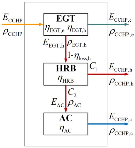
Figure 2. Schematic diagram of the energy–carbon coupling relationship in CCHP.

Energy conversion devices within the energy hub can be categorized into four types: single input–single output, single input–multiple output, multiple input–single output, and multiple input–multiple output. Each energy conversion device is defined as an Energy Conversion Unit (ECU). Special ECUs include energy flow aggregation points and separation points. The energy flow aggregation point gathers multiple energy inputs into a single-energy output, while the energy flow separation point divides a single-energy input into multiple same-type energy flows, which are then directed to the output. The schematic of energy conversion devices within the energy hub is shown in Figure 3.

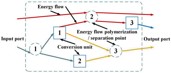
Figure 3. Schematic diagram of energy conversion devices within the energy hub.

Using energy aggregation points and energy separation points as examples, the energy–carbon coupling relationships are analyzed. The schematic diagram of the energy–carbon coupling relationships for the energy aggregation point ECU1 and the energy separation point ECU2 is shown in Figure 4. In energy separation point ECU2, the energy and carbon flow are distributed to two branches, with distribution ratios of ${\eta }_1$ and $1-{\eta }_1$, respectively. The energy and carbon emissions output from ECU2 are illustrated in the figure, and the coupling relationship of energy flow and carbon flow in the ECU still satisfies the carbon emission balance expression, namely:

$$\begin{array}{l}{E}_{\mathrm{Grid}}{\rho }_{\mathrm{Grid}}=\left(E_{\mathrm{Grid}}+E_{\mathrm{PV}}+E_{\mathrm{WT}}\right){\rho }_{\mathrm{Grid},\mathrm{i}}\\ ={\eta }_1\left(E_{\mathrm{Grid}}+E_{\mathrm{PV}}+E_{\mathrm{WT}}\right){\rho }_{\mathrm{Grid},1}+\left(1-{\eta }_1\right)\left(E_{\mathrm{Grid}}+E_{\mathrm{PV}}+E_{\mathrm{WT}}\right){\rho }_{\mathrm{Grid},2}\end{array}$$

(24)

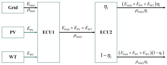
Figure 4. Schematic diagram of the energy–carbon coupling relationship of ECU.

2.3. Energy–Carbon Coupling Model of the Integrated Energy System

The core of energy hub modeling lies in solving the coupling matrix that reflects the conversion and transmission relationships of multi-energy flows and carbon flows between the system’s input and output ports. This paper will progressively solve the multi-part coupling matrix of the integrated energy system based on the constructed partial models. The results of the partial modeling of the integrated energy system are shown in Figure 5.

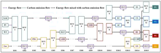
Figure 5. Results of partial modeling of the system.

From Figure 5, it can be observed that EH₁ contains four input ports and two output ports. Based on the known parameters, the coupling matrix C₁ of EH₁ can be determined as follows:

$$C_1=\left[\begin{array}{cccc}1& 1& 1& 0\\ 0& 0& 0& 1\end{array}\right]$$

(25)

Similarly, EH₂ contains two input ports and three output ports. The coupling matrix C₂ of EH₂ can be determined based on the known parameters as follows:

$$C_2=\left[\begin{array}{cc}{\eta }_1& 0\\ 1-{\eta }_1& 0\\ 0& 1\end{array}\right]$$

(26)

EH₃ contains three input ports and three output ports. The coupling matrix C₃ of EH₃ can be determined based on the known parameters as follows:

$$C_3=\left[\begin{array}{ccc}1& 0& 0\\ 0& {\eta }_{\mathrm{P}2\mathrm{G}}& 0\\ 0& 0& 1\end{array}\right]$$

(27)

EH₄ contains three input ports and two output ports. The coupling matrix C₄ of EH₄ can be determined based on the known parameters as follows:

$$C_4=\left[\begin{array}{ccc}1& 0& 0\\ 0& 1& 1\end{array}\right]$$

(28)

EH₅ contains two input ports and four output ports. The coupling matrix C₅ of EH₅ can be determined based on the known parameters as follows:

$$C_5=\left[\begin{array}{cc}1& 0\\ 0& {\eta }_2\\ 0& {\eta }_3\\ 0& 1-{\eta }_2-{\eta }_3\end{array}\right]$$

(29)

EH₆ contains four input ports and four output ports. The coupling matrix C₆ of EH₆ can be determined based on the known parameters as follows:

$$C_6=\left[\begin{array}{cccc}1& 0& 0& 0\\ 0& {\eta }_{\mathrm{EGT}}& 0& 0\\ 0& 0& {\eta }_{\mathrm{GHB}}& 0\\ 0& 0& 0& 1\end{array}\right]$$

(30)

EH₇ contains four input ports and three output ports. The coupling matrix C₇ of EH₇ can be determined based on the known parameters as follows:

$$C_7=\left[\begin{array}{cccc}1& 1& 0& 0\\ 0& 0& 1& 0\\ 0& 0& 0& 1\end{array}\right]$$

(31)

EH₈ contains three input ports and four output ports. The coupling matrix C₈ of EH₈ can be determined based on the known parameters as follows:

$$C_8=\left[\begin{array}{ccc}{\eta }_4& 0& 0\\ 1-{\eta }_4& 0& 0\\ 0& 1& 0\\ 0& 0& 1\end{array}\right]$$

(32)

EH₉ contains four input ports and four output ports. The coupling matrix C₉ of EH₉ can be determined based on the known parameters as follows:

$$C_9=\left[\begin{array}{cccc}1& 0& 0& 0\\ 0& {\eta }_{\mathrm{EGB}}& 0& 0\\ 0& 0& 1& 0\\ 0& 0& 0& 1\end{array}\right]$$

(33)

EH₁₀ consists of four input ports and three output ports. The coupling matrix C₁₀ of EH₁₀ can be derived from the known parameters:

$$C_{10}=\left[\begin{array}{cccc}1& 0& 0& 0\\ 0& 1& 1& 0\\ 0& 0& 0& 1\end{array}\right]$$

(34)

EH₁₁ consists of three input ports and five output ports. The coupling matrix C₁₁ of EH₁₁ can be derived from the known parameters:

$$C_{11}=\left[\begin{array}{ccc}{\eta }_5& 0& 0\\ 1-{\eta }_5& 0& 0\\ 0& {\eta }_6& 0\\ 0& 1-{\eta }_6& 0\\ 0& 0& 1\end{array}\right]$$

(35)

EH₁₂ consists of five input ports and five output ports. The coupling matrix C₁₂ of EH₁₂ can be derived from the known parameters:

$$C_{12}=\left[\begin{array}{ccccc}1& 0& 0& 0& 0\\ 0& {\eta }_{\mathrm{EC}}& 0& 0& 0\\ 0& 0& {\eta }_{\mathrm{AC}}& 0& 0\\ 0& 0& 0& 1& 0\\ 0& 0& 0& 0& 1\end{array}\right]$$

(36)

EH₁₃ consists of five input ports and five output ports. The coupling matrix C₁₃ of EH₁₃ can be derived from the known parameters:

$$C_{13}=\left[\begin{array}{ccccc}1& 0& 0& 0& 0\\ 0& 1& 1& 0& 0\\ 0& 0& 0& 0& 0\\ 0& 0& 0& 1& {\eta }_7\\ 0& 0& 0& 0& 1-{\eta }_7\end{array}\right]$$

(37)

EH₁₄ consists of five input ports and seven output ports. The coupling matrix C₁₄ of EH₁₄ can be derived from the known parameters:

$$C_{14}=\left[\begin{array}{ccccc}{\eta }_{\mathrm{ES}}& 0& 0& 0& 0\\ 0& {\eta }_{\mathrm{CS}}& 0& 0& 0\\ 0& 0& {\eta }_{\mathrm{HS}}& 0& 0\\ 0& 0& 0& {\eta }_{\mathrm{CCHP},\mathrm{e}}& 0\\ 0& 0& 0& {\eta }_{\mathrm{CCHP},\mathrm{c}}& 0\\ 0& 0& 0& {\eta }_{\mathrm{CCHP},\mathrm{h}}& 0\\ 0& 0& 0& 0& {\eta }_{\mathrm{GS}}\end{array}\right]$$

(38)

EH₁₅ consists of seven input ports and four output ports. The coupling matrix C₁₅ of EH₁₅ can be derived from the known parameters:

$$C_{15}=\left[\begin{array}{ccccccc}1& 0& 0& 1& 0& 0& 0\\ 0& 1& 0& 0& 1& 0& 0\\ 0& 0& 1& 0& 0& 1& 0\\ 0& 0& 0& 0& 0& 0& 1\end{array}\right]$$

(39)

To establish the energy hub model of the integrated energy system, it is necessary to solve for the system input vector, output vector, and the coupling matrix that reflects the multi-energy flow conversion relationship between the input and output ports.

First, the system input vector is determined by the elements of the system input ports. Since photovoltaic generation units and wind power generation units do not produce CO₂, the input ports sequentially include the input power from the grid, photovoltaic generation, wind power generation, and the natural gas network, as well as the carbon flow densities from the grid and the natural gas network. The input vector P can be expressed as follows:

$$P=\left[\begin{array}{c}{P}_{\mathrm{grid}}\\ P_{\mathrm{pv}}\\ P_{\mathrm{wt}}\\ P_{\mathrm{gas}}\\ {\rho }_{\mathrm{i},\mathrm{grid}}\\ {\rho }_{\mathrm{i},\mathrm{gas}}\end{array}\right]$$

(40)

In the equation, $P_{\mathrm{grid}}$ represents the input power from the grid, $P_{\mathrm{pv}}$ denotes the input power from photovoltaic generation, $P_{\mathrm{wt}}$ signifies the input power from wind power generation, $P_{\mathrm{gas}}$ indicates the input power from the natural gas network, ${\rho }_{\mathrm{i},\mathrm{grid}}$ represents the carbon flow density from the grid, and ${\rho }_{\mathrm{i},\mathrm{gas}}$ denotes the carbon flow density from the natural gas network.

Similarly, the output vector of the energy hub is determined by the elements of the output ports. The output ports sequentially include the output power for electrical load, thermal load, cooling load, and gas load, along with the corresponding carbon flow densities for electricity, heat, cooling, and gas loads. Therefore, the output vector L can be expressed as follows:

$$L=\left[\begin{array}{c}{P}_{\mathrm{el}}\\ P_{\mathrm{cl}}\\ P_{\mathrm{hl}}\\ P_{\mathrm{gl}}\\ {\rho }_{\mathrm{o},\mathrm{el}}\\ {\rho }_{\mathrm{o},\mathrm{cl}}\\ {\rho }_{\mathrm{o},\mathrm{hl}}\\ {\rho }_{\mathrm{o},\mathrm{gl}}\end{array}\right]$$

(41)

In the equation, $P_{\mathrm{el}}$, $P_{\mathrm{hl}}$, $P_{\mathrm{cl}}$, and $P_{\mathrm{gl}}$ represent the output power of electrical load, thermal load, cooling load, and gas load, respectively, while ${\rho }_{\mathrm{o},\mathrm{el}}$, ${\rho }_{\mathrm{o},\mathrm{hl}}$, ${\rho }_{\mathrm{o},\mathrm{cl}}$, and ${\rho }_{\mathrm{o},\mathrm{gl}}$ denote the carbon flow densities for electricity, heat, cooling, and gas loads, respectively.

Finally, based on the specific sub-model construction of the integrated energy system within the park, the resulting energy–carbon modeling framework for the comprehensive energy system is illustrated in Figure 6, with the formulation for solving the system coupling matrix C derived as follows:

$$C=C_{15}{C}_{14}{C}_{13}\dots C_3{C}_2{C}_1$$

(42)

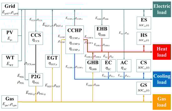
Figure 6. Results of the energy–carbon modeling for the integrated energy system.

By substituting each of the obtained coupling matrices for the respective EH units into Equation (44), the integrated energy hub model for the comprehensive energy system selected in this study is derived as follows:

$$\left[\begin{array}{c}{P}_{\mathrm{el}}\\ P_{\mathrm{cl}}\\ P_{\mathrm{hl}}\\ P_{\mathrm{gl}}\\ {\rho }_{\mathrm{o},\mathrm{el}}\\ {\rho }_{\mathrm{o},\mathrm{cl}}\\ {\rho }_{\mathrm{o},\mathrm{hl}}\\ {\rho }_{\mathrm{o},\mathrm{gl}}\end{array}\right]=\left[\begin{array}{cccccc}{C}_{11}& C_{12}& C_{13}& C_{14}& 0& 0\\ C_{21}& C_{22}& C_{23}& C_{24}& 0& 0\\ C_{31}& C_{32}& C_{33}& C_{34}& 0& 0\\ C_{41}& C_{42}& C_{43}& C_{44}& 0& 0\\ 0& 0& 0& 0& C_{55}& C_{56}\\ 0& 0& 0& 0& C_{65}& C_{66}\\ 0& 0& 0& 0& C_{75}& C_{76}\\ 0& 0& 0& 0& C_{85}& C_{86}\end{array}\right]\left[\begin{array}{c}{P}_{\mathrm{grid}}\\ P_{\mathrm{pv}}\\ P_{\mathrm{wt}}\\ P_{\mathrm{gas}}\\ {\rho }_{\mathrm{i},\mathrm{grid}}\\ {\rho }_{\mathrm{i},\mathrm{gas}}\end{array}\right]$$

(43)

In this equation, C_j represents the coupling matrix of each sub-model within the energy hub, $j\in \left\{1,2,3\dots 14,15\right\}$, while C_mn denotes elements of the comprehensive energy–carbon coupling matrix C for the entire integrated energy system, $m\in \left\{1,2,3\dots 7,8\right\},n\in \left\{1,2,3,4,5,6\right\}$.

Thus, the construction of the energy–carbon coupling model for the energy hub within the integrated energy system is now complete.

3. Low-Carbon Economic Optimal Scheduling Based on Energy–Carbon Coupled Modeling

This paper presents a low-carbon economic optimization method based on energy–carbon coupling modeling. The optimization scheduling framework is shown in Figure 7 and consists of four main steps: (1) constructing the energy–carbon coupling model of the integrated energy system; (2) designing a low-carbon economic optimization scheduling model based on the energy–carbon coupling model; (3) using the PSO algorithm for optimization, generating the Pareto front; (4) finally, applying the TOPSIS multi-objective decision-making algorithm to select the optimal solution and obtain the best operational plan.

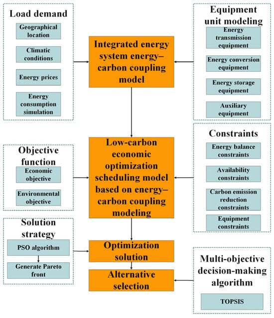
Figure 7. IES optimization process flowchart.

3.1. Objective Function

This study optimizes the scheduling of the integrated energy system, coordinating resources in the electricity, heating, cooling, and gas subsystems to meet load demands and system operation constraints. By optimizing storage devices and employing demand-side management, the objective is to minimize both operating costs and carbon emissions.

3.1.1. System Operating Cost

The operating cost of the integrated energy system includes electricity purchase costs, gas purchase costs, operation and maintenance costs of each device, and curtailment costs associated with photovoltaic and wind power generation units.

$$\begin{array}{l}\min C=C_{\mathrm{ele}}+C_{\mathrm{gas}}+C_{\mathrm{om}}+C_{\mathrm{loss}}\\ C_{\mathrm{ele}}={\displaystyle \sum _{t=1}^T{\lambda }_e}(t)P_{\mathrm{grid}}^{\mathrm{buy}}(t)\\ C_{\mathrm{gas}}={\displaystyle \sum _{t=1}^T{\lambda }_g}(t)P_{\mathrm{gas}}^{\mathrm{buy}}(t)\\ C_{\mathrm{om}}={\displaystyle \sum _{t=1}^T{\displaystyle \sum _{i=1}^N{\lambda }_{om,i}}}{P}_i(t)\\ C_{\mathrm{loss}}={\displaystyle \sum _{t=1}^T[}{\lambda }_{solar}{P}_{solar}^{loss}(t)+{\lambda }_{wind}{P}_{wind}^{loss}(t)]\end{array}$$

(44)

In this equation, C represents the system operating cost; $C_{\mathrm{ele}}$ denotes the cost of electricity purchase; $C_{\mathrm{gas}}$ denotes the cost of gas purchase; $C_{\mathrm{om}}$ represents the operation and maintenance cost of equipment; $C_{\mathrm{loss}}$ represents the cost of curtailed energy; ${\lambda }_e$, ${\lambda }_g$, ${\lambda }_{solar}$, and ${\lambda }_{wind}$ are the electricity purchase price, gas purchase price, curtailed photovoltaic price, and curtailed wind power price, respectively; ${\lambda }_{om,i}$ denotes the operation and maintenance coefficient of the i-th piece of equipment; $P_{\mathrm{grid}}^{\mathrm{buy}}(t)$, $P_{\mathrm{gas}}^{\mathrm{buy}}(t)$, $P_i(t)$, $P_{solar}^{loss}(t)$, and $P_{wind}^{loss}(t)$ represent, respectively, the purchased electricity, purchased gas, output power of the i-th device, curtailed PV power, and curtailed wind power at time t.

3.1.2. System Carbon Emission

The carbon emissions of the integrated energy system consist of the sum of the carbon emissions from the electrical, thermal, cooling, and gas loads at the system load end.

$$\min F={\displaystyle \sum _{t=1}^{24}{\rho }_{\mathrm{o},\mathrm{el},t}{P}_{\mathrm{el},t}}+{\rho }_{\mathrm{o},\mathrm{cl},t}{P}_{\mathrm{cl},t}+{\rho }_{\mathrm{o},\mathrm{hl},t}{P}_{\mathrm{hl},t}+{\rho }_{\mathrm{o},\mathrm{gl},t}{P}_{\mathrm{gl},t}$$

(45)

In the equation, $P_{\mathrm{el},t}$, $P_{\mathrm{hl},t}$, $P_{\mathrm{cl},t}$, and $P_{\mathrm{gl},t}$ represent the output power of the electrical, thermal, cooling, and gas loads at time t, respectively. Meanwhile, ${\rho }_{\mathrm{o},\mathrm{el},t}$, ${\rho }_{\mathrm{o},\mathrm{hl},t}$, ${\rho }_{\mathrm{o},\mathrm{cl},t}$, and ${\rho }_{\mathrm{o},\mathrm{gl},t}$ represent the carbon flux densities of the electrical, thermal, cooling, and gas loads at time t, respectively.

3.2. Constraints

3.2.1. Equipment Power Constraints

$$P_{i,\min }\le P_i(t)\le P_{i,\max }$$

(46)

In this equation, $P_{i,\min }$ and $P_{i,\max }$ represent the upper and lower output limits of the i-th device.

3.2.2. Energy Storage Component’s Periodic Energy Constraints

$$\left\{\begin{array}{l}SO{C}_{i,\min }\le SO{C}_i(t)\le SO{C}_{i,\max }\hfill \\ SO{C}_i(T)=SO{C}_i(0)\hfill \end{array}\right.$$

(47)

In the equation, $SO{C}_{i,\min }$, $SO{C}_{i,\max }$, and $SO{C}_i(0)$ represent the upper and lower limits of the energy storage device i; $SO{C}_i(t)$ denotes the state of energy storage at time t.

3.2.3. Ramp Rate Constraints

$$\left|\begin{array}{c}\mathsf{\Delta }{P}_i\end{array}\right|\le P_{i,climb}$$

(48)

In the equation, $\mathsf{\Delta }P$ represents the output variation of device i; $P_{i,climb}$ denotes the ramp rate of the device.

3.2.4. Interaction Power Constraint Between the Integrated Energy System and the Upper-Level Power Grid and Gas Network

$$\begin{array}{l}0⩽P_{\mathrm{grid}}^{\mathrm{buy}}(t)⩽P_{\mathrm{grid},\max }^{\mathrm{buy}}\\ 0⩽P_{\mathrm{grid}}^{\mathrm{sell}}(t)⩽P_{\mathrm{grid},\max }^{\mathrm{sell}}\\ 0⩽P_{\mathrm{gas}}^{\mathrm{buy}}(t)⩽P_{\mathrm{gas},\max }^{\mathrm{buy}}\\ 0⩽P_{\mathrm{gas}}^{\mathrm{sell}}(t)⩽P_{\mathrm{gas},\max }^{\mathrm{sell}}\end{array}$$

(49)

In the equation, $P_{\mathrm{grid},\max }^{\mathrm{buy}}$ and $P_{\mathrm{grid},\max }^{\mathrm{sell}}$ represent the maximum allowable purchase and sale power between the integrated energy system and the upper-level power grid, while $P_{\mathrm{gas},\max }^{\mathrm{buy}}$ and $P_{\mathrm{gas},\max }^{\mathrm{sell}}$ denote the maximum allowable purchase and sale gas power between the integrated energy system and the upper-level gas network.

3.2.5. Carbon Flow Density Constraint at the Load Side

$$\begin{array}{l}0<{\rho }_{\mathrm{o},\mathrm{el},t}<{\rho }_{\mathrm{o},\mathrm{el},\max }\\ 0<{\rho }_{\mathrm{o},\mathrm{cl},t}<{\rho }_{\mathrm{o},\mathrm{cl},\max }\\ 0<{\rho }_{\mathrm{o},\mathrm{hl},t}<{\rho }_{\mathrm{o},\mathrm{hl},\max }\\ 0<{\rho }_{\mathrm{o},\mathrm{gl},t}<{\rho }_{\mathrm{o},\mathrm{gl},\max }\end{array}$$

(50)

In the equation, ${\rho }_{\mathrm{o},\mathrm{el},\max }$, ${\rho }_{\mathrm{o},\mathrm{cl},\max }$, ${\rho }_{\mathrm{o},\mathrm{hl},\max }$, and ${\rho }_{\mathrm{o},\mathrm{gl},\max }$ represent the upper limit values of the carbon flow densities for electric, cooling, heating, and gas loads, respectively.

3.2.6. Equipment Carbon Emission Constraints

$$0<{\displaystyle \sum _{t=1}^{24}{\rho }_{k,t}{P}_{k,t}}<E_{k,\max },k\in \mathsf{\Omega }$$

(51)

In the equation, $E_{k,\max }$ represents the upper limit of carbon emissions for device k. $\mathsf{\Omega }$ denotes the collection of all energy conversion devices within the park. ${\rho }_{k,t}$ indicates the carbon flow density generated by device k during operation, while $P_{k,t}$ signifies the power output of device k at time t.

4. Results and Discussion

4.1. Basic Data

4.1.1. Low-Carbon Industrial Park Integrated Energy System

The case study in this paper selects a typical low-carbon industrial park integrated energy system as illustrated in Figure 1, which has been improved based on the research in reference [13], focusing on low-carbon economic optimization scheduling. The scheduling period is set to 24 h, with a unit scheduling duration of 1 h. The external electricity purchase price and external gas purchase price are depicted in Figure 8. The full-day output of the wind power units, the full-day output of the photovoltaic units, and the electric, thermal, cooling, and gas load demands of the IES on a typical day are shown in Figure 9.

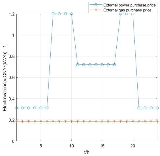
Figure 8. External electricity purchase price and external gas purchase price.

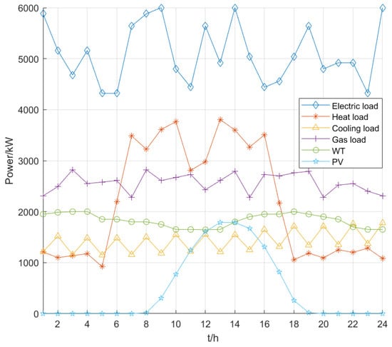
Figure 9. Photovoltaic and wind power output and load demand.

The carbon flow density of electrical energy supplied by the upper-level power grid and the carbon flow density of natural gas supplied by the upper-level gas grid are shown in Figure 10. The carbon flow density of natural gas supplied by the upper-level gas grid remains constant over time. The equipment parameters in the IES are listed in Table 1 [14].

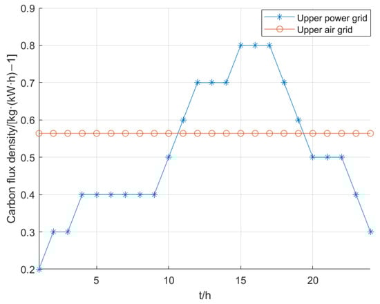
Figure 10. Carbon flow densities of the upper-level power grid and gas network.

Table 1. Equipment parameters of the IES.

Type	Rated Capacity/kW	Efficiency/%	Maximum Climb Rate /(kW·min−1)	Operation and Maintenance Cost (CNY/kW)
EGT	1000 kW	0.33	33.3 kW/min	0.063 CNY/kW
PV	2000 kW	/	/	0.0235 CNY/kW
WT	2000 kW	/	/	0.0196 CNY/kW
GHB	500 kW	0.9	/	0.012 CNY/kW
EHB	500 kW	0.95	/	0.02 CNY/kW
EC	2000 kW	4	/	0.015 CNY/kW
AC	800 kW	0.8	/	1.6 × 10−4 CNY/kW
P2G	4000 kW	0.8	/	0.08 CNY/kW
CCHP	5000 kW	0.3, 1.36, 1.03	/	0.05 CNY/kW
ES	4000 kW	0.95	/	0.0018 CNY/kW
HS	300 kW	0.88	/	0.0016 CNY/kW
CS	300 kW	0.95	/	0.0016 CNY/kW
GS	200 m3	0.95	/	0.0018 CNY/m3

To verify the advantages of the low-carbon economic scheduling model for the IES compared to independent optimization of economic and environmental objectives, three scenarios are selected for this study.

Scenario 1: Coupled scheduling of the four subsystems of the IES—electricity, heating, cooling, and gas—where the objective function considers only the optimization of the system’s operational costs.

Scenario 2: Coupled scheduling of the four subsystems of the IES—electricity, heating, cooling, and gas—where the objective function focuses solely on the optimization of the system’s carbon emissions.

Scenario 3: Coupled scheduling of the four subsystems of the IES—electricity, heating, cooling, and gas—where the objective function accounts for both the operational costs and carbon emissions of the system. This represents the proposed low-carbon economic scheduling model based on energy–carbon coupling modeling.

4.1.2. Integrated Energy System for Commercial Park Buildings

This case study selects a typical integrated energy system for commercial park buildings as shown in Figure 11, with its energy–carbon modeling results depicted in the same figure. The model is improved based on the work in reference [15] for low-carbon economic optimization scheduling. The scheduling period is 24 h per day, with a unit scheduling duration of 1 h. The external electricity purchase price and external natural gas purchase price are shown in Table 2, while the daily output of the photovoltaic units and the electricity, heating, cooling, and gas load demands of the IES on a typical day are illustrated in Figure 12.

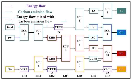
Figure 11. Energy–carbon modeling results of the integrated energy system for commercial park buildings.

Table 2. External electricity and gas purchase prices.

Time	External Electricity Purchase Price (CNY/kW·h)	External Gas Purchase Price (CNY/kW·h)
1:00–8:00	0.41	0.366
9:00–11:00	1.00	0.386
12:00–13:00	0.41	0.366
14:00–18:00	1.00	0.386
19:00–20:00	1.35	0.482
21:00–22:00	1.00	0.386
23:00–24:00	0.41	0.366

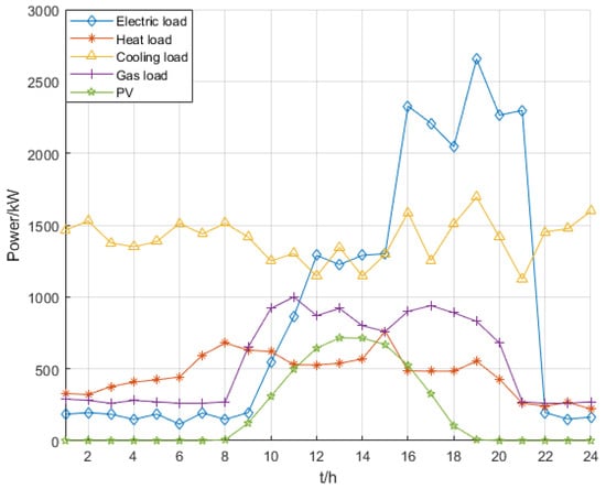
Figure 12. Photovoltaic output and load demand.

The carbon flow density of electricity supplied by the upper-level power grid is set to 0.7921 kg/kW·h, and the carbon flow density of natural gas supplied by the upper-level gas network is set to 0.564 kg/kW·h, both of which remain constant over time. The parameters of the devices within the IES [15] are shown in Table 3.

Table 3. Device parameters of the IES.

Type	Rated Capacity/kW	Efficiency/%	Operation and Maintenance Cost (CNY/kW)
PV	800 kW	/	0.0235 CNY/kW
GHB	550 kW	0.8	0.012 CNY/kW
EHB	400 kW	0.95	0.02 CNY/kW
EC	200 kW	4	0.015 CNY/kW
AC	1000 kW	0.7	16 × 10−5 CNY/kW
CHP	550 kW	0.35, 0.45	0.05 CNY/kW
ES	1500 kW	0.8	0.0018 CNY/kW
HS	130 m3	0.9	0.0016 CNY/kW

4.2. Optimization Scheduling Results Analysis

4.2.1. Research and Discussion on the Optimization Scheduling Results of the Industrial Park

Table 4 presents the optimization results for the three scenarios. It can be observed that in Scenario 3, utilizing the proposed low-carbon economic scheduling model based on energy–carbon coupling modeling, the total operational cost of the system increases by 5058 CNY while reducing carbon emissions by 1328 kg. Although the carbon emissions in Scenario 2 are 978 kg lower than in Scenario 3, the total operational cost of the system in Scenario 2 is 3702 CNY higher than that in Scenario 3.

Table 4. Industrial park optimization results for the three scenarios.

Scenario	Total System Operating Cost/CNY	Equipment Operation and Maintenance Cost/CNY	Cost of Purchasing Electricity/CNY	Cost of Gas Purchase/CNY	Carbon Emission/kg
1	53,882	5508.9	38,978.5	9394.6	85,421
2	62,669	6725.1	46,857.5	9086.4	83,115
3	58,967	5991.1	44,514.8	8461.1	84,093

The operating curve of the power grid is shown in Figure 13. The electricity demand of the industrial park remains stable between 4000 and 6000 kW·h. From 0 to 7 h, the output of photovoltaic power generation is zero, resulting in a higher electricity purchase from the upper grid. This is due to the lack of solar power generation during nighttime, requiring the grid to meet the demand. Between 8 and 18 h, the output of photovoltaic power generation gradually increases, while the electricity demand also rises, leading to an increased electricity purchase from the upper grid. During this time, solar generation helps meet a portion of the demand, but the grid still provides supplementary power. From 19 to 23 h, the electricity demand decreases, and the output of photovoltaic power generation is zero, stabilizing the purchase from the upper grid at around 2500 kW·h. With lower demand in the evening, the grid’s electricity purchase stabilizes. It can be observed from the figure that, through the multi-objective optimization under the low-carbon economic optimal operation mode, the load curve has been optimized compared to the economically optimal operation mode based on fixed electricity for heating, thereby transferring some loads during peak electricity consumption periods to off-peak periods, effectively achieving the peak shaving and valley filling of electricity demand.

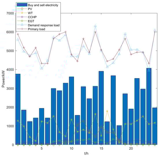
Figure 13. Grid operation curves for industrial park.

The operating curve of the heating network is illustrated in Figure 14. The period from 6:00 to 18:00 represents the peak heating demand. During this time, the heating demand is at its highest, typically corresponding to the morning and evening hours when the industrial park experiences the most significant need for heating. It can be observed that, through the multi-objective optimization under the optimal operation mode of the low-carbon economy, the load curve is smoother compared to the load curve under the economic optimal operation mode based on electricity for heating. This optimization strategy helps to reduce heating peaks and smooth out fluctuations, enhancing system efficiency. The heat storage tank stores heat during the low-demand periods and releases heat during the peak demand periods. By utilizing thermal storage, the system can shift energy use from off-peak to peak periods, reducing the need for additional heating during high-demand hours. At certain moments, the heat output from the CCHP slightly exceeds the heating demand of the industrial park, as some waste heat from the CCHP is absorbed by the absorption chiller, ultimately converting it into cooling load. This is a demonstration of the integrated use of waste heat in the system, which improves overall energy efficiency by simultaneously meeting heating and cooling demands.

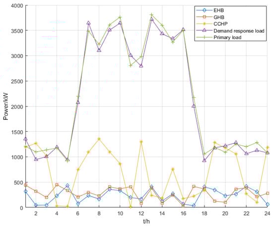
Figure 14. Operating curves of heating networks in industrial park.

The operating curve of the cooling network is shown in Figure 15. The cooling load demand of the industrial park fluctuates between 1000 and 1800 kW·h. This fluctuation is typical of cooling demand, which varies with external temperature changes and occupancy patterns within the industrial park. It can be observed that, through the multi-objective optimization under the low-carbon economic optimal operation mode, the load curve is smoother compared to that of the economic optimal operation mode based on electricity-based heating. The optimization approach reduces sharp spikes in cooling demand, leading to more efficient energy use throughout the day. The cooling storage tank stores cooling during low cooling demand periods and releases cooling during peak cooling demand periods, which helps to alleviate the pressure during peak cooling times to some extent.

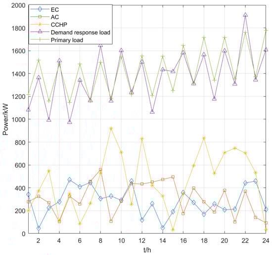
Figure 15. Operating curves of cooling networks in industrial park.

The operating curve of the gas network is shown in Figure 16. The gas load demand of the industrial park remains stable between 2000 and 3000 kW·h. This stable demand is typical of gas usage in the industrial park, which is primarily used for heating and certain industrial processes. It can be observed from the figure that, through the multi-objective optimization under the low-carbon economic optimal operation mode, the load curve is smoother compared to that of the economic optimal operation mode based on electric heating. This smoothing effect is due to the optimization strategy that balances the gas consumption more evenly, avoiding spikes during peak demand periods. At certain times, the quantity of gas purchased from the upper gas network and the gas production from P2G slightly exceed the gas load demand of the industrial park, as a certain amount of gas load is required as input for the CCHP, gas turbine, and gas boiler. The excess gas is stored or used for these energy conversion devices, ensuring that there is enough supply for heating and power generation, especially during high demand.

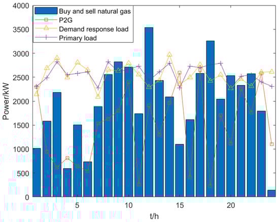
Figure 16. Natural gas network operating curves for industrial park.

The carbon emissions of electricity, heating, cooling, and gas loads, as well as the total carbon emissions of the integrated energy system (IES), are depicted in Figure 17. The carbon emissions from the electricity load are relatively stable overall, with minor fluctuations, maintaining a low level due to the high proportion of clean energy utilized by the grid. This stability is due to the grid’s reliance on renewable energy sources. The carbon emissions from the heating load show a significant upward trend from 6:00 to 18:00, particularly peaking at noon, as this period corresponds to increased heating or hot water demand in buildings, predominantly relying on natural gas as the energy source, leading to a marked rise in carbon emissions with the increase in demand. This peak is driven by higher natural gas use for heating during the day. The carbon emissions from the cooling load fluctuate significantly during the daytime, peaking at noon, which is associated with the cooling demand triggered by rising temperatures. The cooling demand increases during midday, leading to higher emissions. The carbon emissions from the gas load are low and stable, attributable to the relatively stable demand for gas in the system. Gas consumption remains steady, resulting in stable emissions. The total carbon emissions of the IES exhibit a notable increasing trend from 12:00 to 18:00, particularly due to high demand for heating and cooling loads during this period, resulting in increased system carbon emissions. This increase is due to simultaneous high heating and cooling demand. Conversely, the total carbon emissions significantly decrease during early morning and evening off-peak periods, indicating that reduced nighttime load demand leads to lower operational loads for the system’s equipment, thereby reducing carbon emissions. Lower demand during off-peak hours results in reduced emissions.

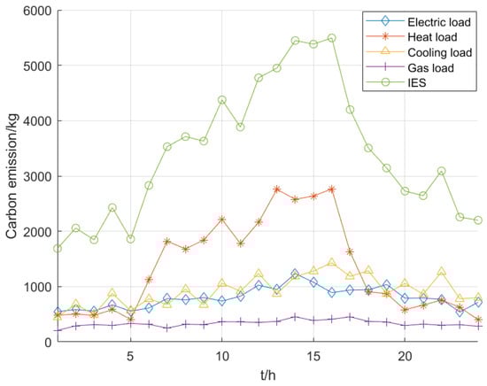
Figure 17. Carbon emission curves of industrial park.

4.2.2. Research and Discussion on the Optimization Scheduling Results of the Commercial Park

Table 5 presents the optimization results for three scenarios. It can be observed that Scenario 3, which adopts the low-carbon economic optimization scheduling model based on energy–carbon coupling proposed in this paper, reduces the system’s carbon emissions by 966 kg while increasing the total operating cost by 1501 CNY. Although the carbon emissions in Scenario 2 are 1381 kg lower than those in Scenario 3, the total operating cost of the system in Scenario 2 is 1785 CNY higher than that in Scenario 3.

Table 5. Commercial park optimization results for the three scenarios.

Scenario	Total System Operating Cost/CNY	Equipment Operation and Maintenance Cost/CNY	Cost of Purchasing Electricity/CNY	Cost of Gas Purchase/CNY	Carbon Emission/kg
1	15,657	469.1	12,400	2787.9	32,699
2	18,943	552.9	15,108	3282.1	30,352
3	17,158	491.3	13,133	3533.7	31,733

The grid operation curve is shown in Figure 18. The electricity load demand in the commercial park fluctuates between 100 and 2700 kW·h. From 0 to 7 h, the PV power generation output is zero, resulting in a higher electricity purchase from the upper grid. From 8 to 21 h, the PV power generation output gradually increases, and as the commercial park starts its operations, the electricity load demand also gradually increases, leading to a rise in electricity purchases from the upper grid. From 22 to 23 h, the electricity load demand decreases, the PV output remains at zero, and the electricity purchase from the upper grid stabilizes at around 1200 kW·h. The electricity demand in the commercial park shows a clear time correlation with the PV power output. When the PV power generation is insufficient, the demand for electricity from the upper grid increases; when the PV generation is sufficient, the electricity purchase demand decreases but still increases with business activities. Optimizing the collaborative operation of PV generation and electricity purchase from the grid is of great significance in improving energy efficiency and reducing electricity purchase costs [16].

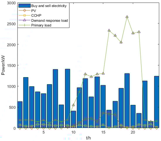
Figure 18. Grid operating curves for commercial park.

The heating network operation curve is shown in Figure 19. From 7 to 19 h is the heating peak. The thermal energy storage tank stores heat during low-demand periods and releases it during peak demand. At certain times, the heat output from the gas boiler slightly exceeds the heating load of the industrial park, as some waste heat from the gas boiler is absorbed by the absorption chiller and converted into cooling load. The curve shows that the thermal energy storage tank effectively balances energy over time, easing the supply–demand pressure during peak heating. Additionally, the gas boiler efficiently meets the heating demand while also providing cooling through the absorption chiller, achieving comprehensive thermal energy utilization. This combined heating and cooling approach improves energy efficiency and supports the park’s low-carbon operation [17].

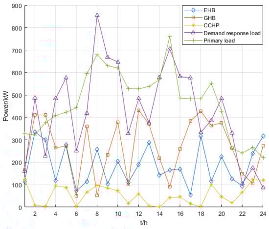
Figure 19. Operating curves of heating networks in commercial park.

The cooling network operation curve is shown in Figure 20. The cooling load demand of the industrial park fluctuates between 1000 and 1800 kW·h. Through the multi-objective optimization of the low-carbon economic optimal operation model, the cooling network load curve is smoother compared to the economic operation model based on electric heating. This indicates that the system has fully accounted for variations in cooling load demand during the optimization scheduling, achieving a balanced distribution and stable operation of the cooling network load. This contributes to improving the overall operational efficiency and energy utilization of the cooling network.

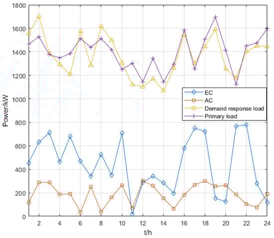
Figure 20. Operating curves of cooling networks in commercial park.

The gas network operation curve is shown in Figure 21. The gas load demand of the industrial park fluctuates between 200 and 1000 kW·h. From 0 to 7 h, the gas purchase from the upper-level gas network increases significantly, exceeding the gas load demand. This is primarily due to the operation of the CHP and gas boilers to meet certain amounts of electricity and heat load demands. The multi-objective optimization of the low-carbon economic optimal operation model results in a smoother gas load curve compared to the economic operation model based on electric heating. However, with the introduction of demand response, the fluctuation amplitude of the gas load has increased slightly to balance the electricity load, reflecting the regulatory effect of the electricity–gas-coordinated optimization scheduling on the overall operation of the system.

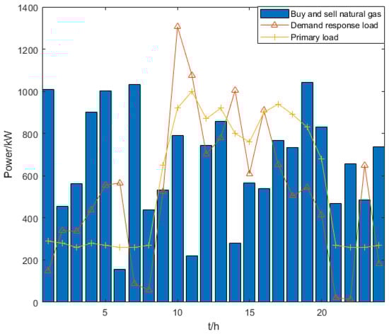
Figure 21. Natural gas network operating curves for commercial park.

Figure 22 illustrates the variation trends of carbon emissions from electricity, heat, cooling, and gas loads, as well as the total carbon emissions of the IES. It can be observed that carbon emissions from electricity and cooling loads fluctuate minimally and remain at a relatively low level, while carbon emissions from heating and gas loads fluctuate significantly, particularly during peak periods. This indicates that heating and gas equipment have a more pronounced impact on carbon emissions. The total carbon emissions of the integrated energy system exhibit a clear daily variation pattern, with higher emissions during daytime peak periods and a decrease during nighttime off-peak periods. This reflects the impact of load aggregation on carbon emissions. By optimizing the scheduling strategy of the integrated energy system and coordinating the operation of various loads, not only can peak carbon emissions be reduced, but the overall carbon emission level can also be effectively lowered. The experimental results show that through multi-energy complementarity and demand response, the energy utilization efficiency of the park can be improved, achieving low-carbon operation and providing effective support for the park’s green development.

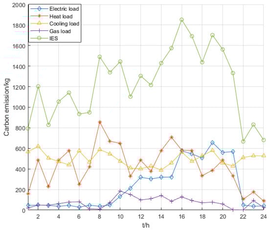
Figure 22. Carbon emission curves of commercial park.

4.3. Discussion

This study proposes an energy–carbon coupling model based on an energy hub and demonstrates its significant advantages across different regions and diverse energy structures through modeling and optimization experiments on the integrated energy systems of industrial low-carbon parks and commercial building complexes. The model promotes an in-depth implementation of sustainable development concepts in the energy sector. The proposed model exhibits exceptional regional adaptability: in industrial parks with high and stable energy demand, it ensures the continuous supply of production energy effectively. In commercial parks, where load fluctuations are significant due to business activities, the model flexibly accommodates dynamic load demands, providing efficient energy optimization strategies that significantly reduce resource waste and environmental impact, thereby facilitating the sustainable utilization of energy. By combining experiments on both types of parks, this research offers multi-scenario comparative validation, systematically testing the model’s accuracy and effectiveness in both depth and breadth. It also identifies potential areas for improvement, further enhancing the model’s reliability in practical applications. The practical experiences gained in this study provide valuable references for systems with similar regional characteristics and energy structures, contributing not only to improving operational efficiency and stability in the energy industry but also to reducing carbon emissions and achieving harmony between energy and the environment. The research results highlight the broad application prospects and critical reference value of the model in optimizing low-carbon energy systems, offering substantial support for the implementation of sustainable development initiatives.

Compared with existing studies, this research surpasses the limitations of single-energy or carbon flow modeling by delving into the intricate coupling relationships among various energy conversion devices and demonstrating the feasibility of integrated optimization. However, the current optimization strategy still faces several limitations, including a high dependency on data, insufficient capability to handle uncertainties, simplifications in equipment operational characteristics, and limited adaptability to market price fluctuations. Future research should aim to enhance the model’s ability to address uncertainties, strengthen real-time monitoring and adaptive control capabilities, and develop dynamic models to investigate equipment degradation patterns and maintenance strategies in greater depth. Moreover, expanding the forms of energy and system scale could integrate emerging energy sources such as hydrogen into the system framework and extend the model’s application to city-level and larger integrated energy systems. By incorporating advanced technologies such as smart grids, the Internet of Things, and artificial intelligence, precise data acquisition and improved intelligence levels can be leveraged to explore the model’s scalability and its deep integration with emerging technologies. This would provide more comprehensive and efficient solutions for low-carbon economic optimization, supporting the transition toward sustainable energy development.

5. Conclusions

This paper proposes an energy–carbon coupling model suitable for the low-carbon economic optimization dispatch of integrated energy systems based on the energy hub modeling method. Firstly, by constructing the energy–carbon coupling model of the integrated energy system, the complex coupling relationships between energy flows and carbon flows among the system’s devices were analyzed in depth, addressing the shortcomings of existing models that only focus on the separate modeling of energy flows or carbon flows. This model not only leverages the advantages of multi-energy integration and conversion but also facilitates the joint modeling of energy flows and carbon flows, along with comprehensive lifecycle carbon emission management, making the calculations of energy and carbon emissions more accurate and consistent. Secondly, based on this model, this paper conducts a low-carbon economic optimization dispatch of the integrated energy system. Through reasonable energy allocation and dispatch strategies, this approach effectively controls economic costs while achieving low-carbon objectives, fully embodying the concept of sustainable development. Finally, the validity of the energy–carbon coupling modeling was verified through case analysis, further demonstrating the model’s applicability in the low-carbon economic optimization dispatch of integrated energy systems. It provides an effective modeling solution for low-carbon parks with multiple energy forms, showcasing promising application prospects.

References

- Chen, S.; Wei, Z.; Gu, W.; Guo, Q. Transformation and change of energy system under carbon neutral target: Multi-energy flow synergy technology. Power Autom. Equip. 2021, 41, 3–12. [Google Scholar]
- Song, D.; Meng, W.; Dong, M.; Yang, J.; Wang, J.; Chen, X.; Huang, L. A critical survey of integrated energy system: Summaries, methodologies and analysis. Energy Convers. Manag. 2022, 266, 115863. [Google Scholar] [CrossRef]
- Lv, G.; Cao, B.; Jun, L.; Liu, G.; Ding, Y.; Yu, J.; Zang, Y.; Zhang, D. Optimal scheduling of integrated energy system under the background of carbon neutrality. Energy Rep. 2022, 8, 1236–1248. [Google Scholar] [CrossRef]
- Xiong, Y.; Chen, L.; Zheng, T.; Si, Y.; Mei, S. Optimized allocation of hydrogen energy storage for integrated energy system in low carbon park considering coupling characteristics of electricity, heat and gas. Power Autom. Equip. 2021, 41, 31–38. [Google Scholar]
- Geidl, M.; Koeppel, G.; Favre-Perrod, P.; Klockl, B.; Andersson, G.; Frohlich, K. Energy hubs for the future. IEEE Power Energy Mag. 2007, 5, 24–30. [Google Scholar] [CrossRef]
- Evins, R. Multi-level optimization of building design, energy system sizing and operation. Energy 2015, 90, 1775–1789. [Google Scholar] [CrossRef]
- Zhang, W. Research on Optimal Scheduling of Multi-Energy Flow System Containing Uncertain Energy Access. Master’s Thesis, North China Electric Power University, Beijing, China, 2020. [Google Scholar]
- Cheng, Y.; Zhang, N.; Wang, Y.; Yang, J.; Kang, C.; Xia, Q. Modeling carbon emission flow in multiple energy systems. IEEE Trans. Smart Grid 2018, 10, 3562–3574. [Google Scholar] [CrossRef]
- Sun, Q.; Xie, D.; Nie, Q.; Zhang, L.; Chen, Q.; Chen, J. Study on economic optimal dispatch of integrated energy system in park with electricity-heat-cooling-gas load. China Electr. Power 2020, 53, 79–88. [Google Scholar]
- Dupont, B.; Dietrich, K.; DeJonghe, C.; Ramos, A.; Belmans, R. Impact of residential demand response on power system operation: A Belgian case study. Appl. Energy 2014, 122, 1–10. [Google Scholar] [CrossRef]
- Yang, Y.; Yi, W.; Wang, C.; Wang, M.; Wu, Z.; Mu, Y.; Zheng, M. Low-carbon economic dispatch of integrated energy system in park based on carbon emission flow theory. Electr. Power Constr. 2022, 43, 33–41. [Google Scholar]
- Song, Y.; Mu, H.; Li, N.; Wang, H.; Kong, X. Optimal scheduling of zero-carbon integrated energy system considering long-and short-term energy storages, demand response, and uncertainty. J. Clean. Prod. 2024, 435, 140393. [Google Scholar] [CrossRef]
- Wang, R.; Sun, Q.; Hu, W.; Zhang, H.; Wang, P. A new type of power system trend calculation for “carbon peak and carbon neutral”. Glob. Energy Internet 2022, 5, 439–446. [Google Scholar]
- Huang, Y.; Sun, Q.; Li, Y.; Gao, W.; Gao, D.W. A multi-rate dynamic energy flow analysis method for integrated electricity-gas-heat system with different time-scale. IEEE Trans. Power Deliv. 2022, 38, 231–243. [Google Scholar] [CrossRef]
- Yang, J. Research on Low-Carbon and Economic Operation Scheduling Method of Regional Multi-Body Building Integrated Energy System. Master’s Thesis, Hangzhou University of Electronic Science and Technology, Hangzhou, China, 2024. [Google Scholar]
- Yang, L.; Li, X.; Sun, M.; Sun, C. Hybrid policy-based reinforcement learning of adaptive energy management for the Energy transmission-constrained island group. IEEE Trans. Ind. Inform. 2023, 19, 10751–10762. [Google Scholar] [CrossRef]
- Luo, Y.; Zeng, B.; Zhang, W.; Liu, Y.; Shi, Q.; Liu, W. Coordinative Planning of Public Transport Electrification, RESs and Energy Networks for Decarbonization of Urban Multi-Energy Systems: A Government-Market Dual-Driven Framework. IEEE Trans. Sustain. Energy 2023, 15, 538–555. [Google Scholar] [CrossRef]
Disclaimer/Publisher’s Note: The statements, opinions and data contained in all publications are solely those of the individual author(s) and contributor(s) and not of MDPI and/or the editor(s). MDPI and/or the editor(s) disclaim responsibility for any injury to people or property resulting from any ideas, methods, instructions or products referred to in the content. |
© 2025 by the authors. Licensee MDPI, Basel, Switzerland. This article is an open access article distributed under the terms and conditions of the Creative Commons Attribution (CC BY) license (https://creativecommons.org/licenses/by/4.0/).