Optimal Strategy and Performance for a Closed-Loop Supply Chain with Different Channel Leadership and Cap-and-Trade Regulation

Abstract

Cap-and-trade is widely recognized as an effective mechanism for curbing carbon emissions, and it significantly influences the operational decisions within supply chains. This study investigates a three-echelon closed-loop supply chain (CLSC) consisting of one original equipment manufacturer, one traditional retailer, and one independent third-party collector. The manufacturer invests in cleaner technologies to produce green products and remanufactures new products from used items recycled by the third-party collector. Considering different channel power structures, three Stackelberg game models are developed, and their optimal solutions are derived using the backward induction. Additionally, the combined effects of remanufacturing-related and carbon-related parameters on economic and environmental benefits as well as social welfare are investigated under different settings. Moreover, the derived results are validated via numerical simulation. The findings indicate that: (1) Each channel member is incentivized to act as the leader role within the CLSC to maximize profits. (2) A loose cap-and-trade regulation is conducive to enhancing the emission abatement rate, collection rate, and overall performance for the CLSC. (3) The retailer-led model is the best option for capturing more economic benefits and social welfare, while the third party-led model can always achieve the best environmental performance regardless of carbon trading price. These research findings can provide valuable insights for policymakers and decision makers engaged in CLSC.

1. Introduction

Environmental deterioration and the greenhouse effect are becoming more severe due to excessive greenhouse gas emissions and environmental pollution. To pursue sustainable development, many countries have issued carbon control legislations to curb carbon emissions by using emission-reducing materials and cleaner production technologies, including European countries, Japan, India, China, etc. [1,2]. In particular, cap-and-trade regulation is regarded as one of the most effective mechanisms to restrict carbon emissions. It is a market-based mechanism to directly limit the quantity of carbon dioxide emissions [3,4,5]. Under this carbon regulation policy, government agencies initially allocate a specific carbon quota to individual enterprises (called the carbon cap), and the carbon emission credits can be traded through the carbon trading market based on the emissions released by the enterprises in the latter operational age [6].

The government’s emission regulation policies significantly impact enterprises’ operations management, forcing them to optimize their operational strategies to balance economic and environmental benefits [5]. In response to cap-and-trade regulation, an increasing number of manufacturers make more effort to reduce carbon emissions by adopting green technologies and establishing reverse logistics and remanufacturing systems [7]. For instance, many automakers, including General, Tesla, and BYD Motors, have engaged in developing clean engines and new energy vehicles. In addition, in the fast fashion industry, H&M, Mark&Spencer, and Levi’s are investing in low-carbon technologies to produce greener products [2,8]. As a case in point, in October 2020, H&M launched a new clothing recycling system “LOOP” in Sweden so as to achieve a positive impact on the climate [9]. Therefore, it is critical to establish mathematical models to evaluate the influence of cap-and-trade regulation on the firms’ pricing, emission abatement decision, and performance under the CLSC framework.

In practice, CLSC is regarded as an effective method for curbing carbon emissions and saving production costs, and has been widely recognized by both practitioners and academics [10,11,12]. As an eco-friendly production manner, it can not only create additional value from used items but also reduce carbon emissions during the manufacturing process [13]. Many leading firms are committed to operating remanufacturing systems by building reverse supply chains, such as Apple, Hewlett-Packard, Canon, Xerox, Caterpillar and Huawei, etc. [14,15]. For instance, Xerox saved 40–65% of its production costs by implementing a recycling program [16], and Volkswagen decreased production costs by 70% by collecting used automobile engines and parts [2]. In addition, Apple has launched a trade-in program for reusing and recycling used products, and its carbon emissions associated with aluminum were decreased by 72% by recycling aluminum in 2020 [17,18]. Therefore, to promote the sustainability development of CLSC, it is essential and urgent to examine how carbon control regulations affect remanufacturing and emission abatement decisions in the context of CLSC, while such questions need to be studied further considering the cap-and-trade policy.

In reality, the cap-and-trade policy and remanufacturing are complementary processes, and the policy is beneficial to the remanufacturing industry [19]. Hence, it is crucial to examine the joint effects of cap-and-trade regulation and remanufacturing on economic and environmental benefits for the CLSC. Even though several previous works have discussed the interactions between remanufacturing and cap-and-trade regulations within the CLSC context, those studies only considered the situation where the manufacturer dominates the CLSC [20]. Although an increasing number of studies are examining how cap-and-trade regulation affects optimal solutions and performance of CLSC, most of them only focus on the case where the manufacturer dominates the whole supply chain, while our study aims to investigate the simultaneous effects of different channel power structures and cap-and-trade regulation on the operations management of the CLSC, particularly in the presence of sustainability investment.

In addition, different agents have charged different channel powers in supply chain, and this can exert great impacts on operational decisions and performance of channel members [21]. Several previous works have studied the effects of channel leadership on optimal strategies within the CLSC framework [22,23,24]; however, none of them have been considered the cap-and-trade regulation policy and emission abatement decisions. Nonetheless, our study takes the manufacturer’s emission abatement decision into account with different Stackelberg game models due to sustainability investment playing an essential role in coping with rigorous carbon emission regulations. Some references are closer to our study, including Zhou et al. [25], Zhang et al. [26], and Yang et al. [27], but those works did not integrate channel leadership and cap-and-trade regulation into a remanufacturing CLSC with third-party collection, whereas our study focuses on investigating the interactions among those factors.

This paper aims to address the following research questions:

• What are the equilibrium outcomes of the three Stackelberg game models associated with different channel power structures and cap-and-trade regulation?
• How do remanufacturing-related and carbon-related parameters jointly affect the optimal pricing, collection, and emission reduction decisions of channel members, as well as supply chain profitability, total carbon emissions, and social welfare of the CLSC?
• Which proposed model is the best choice in terms of economic and environmental benefits as well as social welfare, respectively?

To address the above questions, we formulated three different Stackelberg game models within a CLSC in which a third-party collector is responsible for recycling used items. Moreover, the joint effects of remanufacturing, channel power structures, and cap-and-trade regulation on optimal equilibrium solutions, profitability, total carbon emissions, and the social welfare of the proposed models are examined. Furthermore, we identified which proposed model is the best option in terms of economic and environmental benefits as well as social welfare, respectively, by conducting comparative analysis and numerical experiments. The findings indicate that remanufacturing is conducive to improving the emission reduction rate, channel members’ profits, and social welfare of the CLSC. Each channel member is motivated to dominate the overall CLSC, while there is no proposed model that can always achieve the best environmental performance. The retailer-led model demonstrates superior economic benefits and social welfare compared to the other two models.

The innovations and contributions of this paper lie in the following two aspects:

• In contrast to the previous literature, our work constructs three Stackelberg game models that correspond to different channel power structures in a CLSC involving third-party collection, and the optimal equilibrium outcomes of the proposed models are systematically analyzed and compared. The derived research conclusions are beneficial to the decision makers with a better understanding of their competitive strategies under different scenarios.
• Most of the previous works have not considered cap-and-trade regulation and different channel power structures simultaneously within a CLSC, whereas our study not only examines the simultaneous impacts of remanufactured-related and carbon-related parameters on economic and environmental benefits as well as social welfare, but also identifies the optimal choice for channel members from different perspectives.

The remainder of this paper is organized as follows. Section 2 reviews the relevant literature. Section 3 describes the problem, model formulation, and analysis. The comparative analysis is proposed in Section 4, and Section 5 describes the numerical experiments. Section 6 first summarizes the conclusions and managerial insights, then ends the paper with conclusions and future research directions. All proofs are presented in Appendix A, Appendix B, Appendix C and Appendix D.

2. Literature Review

Our study is closely related to two research streams: one is the CLSC with cap-and-trade regulation, and the other is operations management of the CLSC involving different channel power structures.

2.1. Remanufacturing CLSC with Cap-and-Trade Regulation

Recently, studies on CLSC management under the cap-and-trade regulation have received considerable attention from scholars [20,27]. Some works have discussed the influence of cap-and-trade regulation on remanufacturing, emission reductions, and pricing decisions. Yang et al. [13] analyzed the effect of cap-and-trade regulation on a CLSC where the take-back process is overtaken by different participants, i.e., the manufacturer, retailer, and third-party collector. The results found that remanufacturing can effectively improve the emission reduction efforts and profits of the manufacturer and retailer. Mondal and Giri [11] developed one centralized and three manufacturer-led decentralized game models in a green CLSC considering governmental intervention and cap-and-trade regulation policies. The analysis demonstrated that both the government subsidies and cap-and-trade policies are profitable to all channel members. Wang and Wu [19] explored emission reduction and collection strategies considering cap-and-trade regulation and consumer environmental awareness when different agents led the collection. The results found that when the parameters met a certain condition, the manufacturer leading the collection was conducive to improving the return rate, emission reduction rate, and profit for the whole supply chain.

In addition, several scholars have investigated the combined effects of carbon control policies or governmental green subsidies on the operations decisions of CLSCs. Cheng et al. [14] studied a CLSC network including the low-emission manufacturers and high-emission manufacturers under the carbon tax and cap-and-trade regulations. The optimal strategies of the CLSC network are analyzed with the assumption that the new and remanufactured products are homogeneous. Lyu et al. [2] systematically investigated the impacts of the cap-and-trade, strict carbon cap, and carbon tax policies on the manufacturer’s recycling and emission reduction decisions. The results showed that the manufacturer is inclined to the carbon tax or cap-and-trade, but never prefers a strict carbon cap. Chai et al. [28] developed three stylized models to analyze the effects of the government subsidy policy and the carbon cap-and-trade policy on remanufacturing in a CLSC. The research results indicated that both the government subsidy policy and the cap-and-trade policy are able to promote remanufacturing.

The above-mentioned literature discussed the interactions between cap-and-trade regulation and remanufacturing within the CLSC context. However, those studies neglected the effects of channel power structures on the operational decisions and performance of channel members, whereas our research centers on formulating three third-party collection models associated with different channel leaderships using two-stage Stackelberg game theory.

2.2. CLSCs Involving Different Channel Power Structures

Many scholars have paid enormous attention to optimal pricing, and performance with the manufacture dominates entire closed-loop supply chains [29,30,31,32]. Nevertheless, those employed studies are only concerned with the situations where the manufacturer dominates the whole supply chain, resulting in limited managerial insights. However, to a great extent, channel power structure has a substantial effect on the acquisition efficiency and even on the performance of the entire CLSC [33].

Several previous works have discussed the impacts of different channel leadership on the operational decisions of the CLSCs [34,35,36]. Gao et al. [22] investigated the influence of different channel power structures on the optimal pricing, collection, and sale effort decisions, as well as the performance of the CLSC. The outcomes showed that the CLSC with a dominant retailer is the most profitable when the demand expansion effectiveness of the collection effort is relatively high. Zheng et al. [37] examined the effects of forward channel competition and different power structures on a dual-channel closed-loop supply chain where the third-party takes charge of the take-back process. A centralized model and three decentralized models, viz., the manufacturer-led, retailer-led, and collector-led models, are analyzed. The results revealed that each channel member has an incentive to play the channel leader’s role. Ranjbar et al. [24] considered a three-level closed-loop supply chain consisting of a manufacturer, a retailer, and a third-party collector, and the optimal pricing and collection decisions associated with different leadership with retailer collecting and third-party collecting were evaluated. They pointed out that the retailer leadership model is often the most effective scenario in CLSC. Wang et al. [38] studied a three-echelon CLSC considering corporate social responsibility and retailers’ sales efforts under information symmetry and information asymmetry situations, and three Stackelberg game models with the third-party collection were constructed and analyzed under different channel power structures. Suvadarshini et al. [39] studied a multi-channel supply chain where the OEM designed an efficient multi-channel recollection structure in which recollection agents competitively recollect used products. The effects of competition, collection efficiencies, individual rationality, and information asymmetry on the optimal equilibrium solutions of the CLSC were analyzed.

The aforesaid literature discussed optimal pricing, reverse channel selection, and performance of the CLSCs with different channel leadership, and most of them involved third-party recycling or third-party-led settings. However, the abovementioned works did not discuss the optimal pricing and emission reduction decisions or performance in the presence of the cap-and-trade policy under different situations.

2.3. Research Gaps

Based on observations from current and extant literature, the existing research gaps are summarized as follows:

• Although some prior works have discussed the optimal pricing and performance of CLSCs under different channel leadership, most have ignored the effect of cap-and-trade regulation on the optimal solutions and performance of the channel members and have not considered third-party collecting. In reality, cap-and-trade regulation significantly influences the operational efficiency of CLSCs, and third-party collectors play a vital role in recycling and remanufacturing processes.
• Several prior studies have explored the optimal emission reduction decisions and performance of the CLSCs in light of the cap-and-trade regulation policy. However, few works have investigated the combined effects of remanufacturing-related and carbon-related parameters on economic and environmental benefits, or social welfare under different CLSC settings.

To address these research questions, we integrated cap-and-trade regulation into a CLSC framework in which the third-party collector is responsible for collecting end-of-life products under different circumstances. We also established three Stackelberg game models in the context of CLSCs. Furthermore, we investigated the optimal equilibrium solutions, economic and environmental benefits, and social welfare of the proposed models via numerical simulations.

Table 1. Summary of relevant papers and the position of our study.

Research Paper	Stackelberg Game	Green Investment	CPT	CLSC	Third-Party Collection
Wang et al. [34]	√			√	√
Zheng et al. [37]	√			√	√
Zerang et al. [40]	√			√	√
Ranjbar et al. [24]	√			√	√
Liu et al. [29]				√	√
Yang et al. [13]	√	√	√	√	√
Lyu et al. [2]	√	√	√	√
Zhang et al. [12]		√		√	√
Wang et al. [38]	√			√	√
Mondal and Giri [22]		√	√	√
Cheng et al. [14]		√	√	√
Zhang et al. [26]		√	√	√	√
Wang et al. [41]	√	√	√	√
Fang et al. [6]	√	√	√	√
Present research	√	√	√	√	√

CLSC: closed-loop supply chain; CPT: cap-and-trade. In addition, √ indicates that the corresponding study related to this main factor.

summarizes the distinctions between previous studies and our work.

3. Model Construction and Analysis

In this section, we investigate a CLSC consisting of a manufacturer, a retailer, and a third-party collector considering different types of channel leadership and cap-and-trade regulation. In the forward supply chain, the manufacturer produces green products using eco-friendly technology to curb carbon emissions, then wholesales the green product to the downstream retailer, who is responsible for selling them to meet the consumer demand in the end market. In the reverse supply chain, the manufacturer subcontracts an independent third-party collector to recycle end-of-life products for the remanufacturing process. The CLSC framework is described as follows (Figure 1):

3.1. Notation

The model notations used throughout the paper are summarized in

Table 2. Definition of variables and parameters.

Symbol	Explanation
w	The wholesale price per unit product (USD, decision variable)
p	The retail price per unit product (USD, decision variable)
e	The emission reduction rate per unit product (decision variable), 0 < e < 1
τ	The return rate of used products (decision variable), 0 < τ < 1
$b$	The transfer price of the manufacturer to the third-party collector for per unit used product (USD, decision variable)
$c_n$	The marginal cost of the new product with raw materials (USD)
$c_r$	The marginal cost of the remanufactured product with used items (USD) $0<c_r<c_n$
$\Delta$	The production cost savings of remanufacturing a new product with used products (USD), $\Delta =c_n-c_r$
$m$	The carbon trading price (USD/ton)
$\lambda$	The emission intensity of unit remanufactured product, $\lambda \in \left(0, 1\right)$; the larger $\lambda$ denotes the more carbon emissions released in the remanufacturing process
$e_0$	The initial carbon emission for per unit product (ton)
$g$	The carbon quota for per unit product (ton)
$\varphi$	The base market demand (unit/year))
$\beta$	The price sensitivity to the market demand
$B$	The coefficient of collection cost ($\mathrm{USD}/{\mathrm{t}\mathrm{o}\mathrm{n}}^2$)
$k$	The coefficient of emission reduction cost ($\mathrm{USD}/{\mathrm{t}\mathrm{o}\mathrm{n}}^2$)
$s$	Total cost savings from remanufacturing a new product with used items (USD), $s=\Delta +m{e}_0\left(1-\lambda \right)$
${ \pi }_i^j$	The channel member’s profit, the subscripted $i\in \left\{m, r, t, s\right\}$ represents the manufacturer, retailer, third-party collector and the whole CLSC respectively; the superscripted $j\in \left\{M, R, T\right\}$ represents the manufacturer-led, retailer-led, and third-party-led game models, respectively
${ E}^j$	The total carbon emissions of different Stackelberg game models (ton)
${SW}^j$	The social welfare of different Stackelberg game models

for clarity.

3.2. Assumptions

To guarantee the validity of the proposed models, several necessary assumptions are presented as follows.

Assumption 1.

The demand function is linear and deterministic, expressed as $D\left(p\right)=\varphi -\beta p$. Note that this type of demand function is widely applied and well established in supply chain management [13,42]. Additionally, to guarantee that market demand in each model and the channel members’ profits remain positive, we assume that $\varphi >\beta p$,  $p>w>c_n+m\left(e_0-g\right)$.

Assumption 2.

Consumers perceive the value of remanufactured products to be equivalent to that of new ones because both types of products serve the same function and appearance. Consequently, the willingness to pay for the new and remanufactured products is assumed to be equal [11,16,43,44].

Assumption 3.

Assume that $s\ge b>A$, where $A$ denotes the unit collection cost that the third party pays for the consumer. For simplicity, $A$ is supposed to be zero, and it is noted that this assumption does not influence the conclusions derived in our study [37]. Furthermore, the above inequality implies that the total cost savings from remanufacturing a new product using used products should not be less than the unit transfer payment that the manufacturer pays to the third-party collector [28].

Assumption 4.

The sustainable investment cost is a quadratic function with respect to the emission reduction rate, which is characterized as $I\left(e\right)=k{e}^2/2$. $k$ is an investment scaling parameter [40,45,46]. Similarly, the collection cost function of the third-party collector is expressed as $I\left(\tau \right)=B{\tau }^2$ [47,48], which reflects the economic relationship between collection cost and the return rate of used products. According to prior literature [25,49], the parameters $k$ and $B$ are supposed to be sufficiently large to ensure the existence of an interior equilibrium solution for each game model, i.e., $k>max\left\{{\displaystyle \frac{B\beta m^2+bk\beta \left(\Delta -b+m{e}_0\left(1-\lambda \right)\right)}{2B}},\beta m^2\right\}$, $B>{\displaystyle \frac{k\left(\Delta +e_0\left(m-m\lambda \right)\right)\left(2\beta \left(\Delta +e_0\left(m-m\lambda \right)\right)+\varphi -\beta c_n-\left(e_0-g\right)m\beta \right)}{8\left(2k-m^2\beta \right)}}$.

Assumption 5.

Under cap-and-trade regulation, the manufacturers can purchase (sell) carbon credit in the carbon trading market when their emissions are greater (smaller) than their carbon quota. Without loss of generality, we assume that the purchasing and selling prices of a unit carbon credit are identical [26,50].

Assumption 6.

The carbon emissions of a unit remanufactured product are $\lambda$ percent of those of a new product during the production process. The value of $\lambda$ is influenced by various factors, such as the manufacturer’s remanufacturing technology, the product’s recycling ability and its physical properties [13]. Since the original carbon emissions per unit of a new product are $e_0$, the unit remanufactured product’s emissions are equal to $\lambda e_0$. Furthermore, the average carbon emissions for producing a unit green product is represented by $\overline{e}=e_0\left(1-\tau \right)+\lambda e_0\tau -e=e_0\left(1+\lambda \tau -\tau \right)-e$, and total carbon emission is a linear function with respect to the market demand, i.e., $E^j=\overline{e}{D}^j$ [51,52].

In the following, we focus on developing three Stackelberg game models in which the third-party collector is responsible for recycling used products under different channel power structures and cap-and-trade regulation, i.e., the manufacturer-led model, the retailer-led model, and the third-party-led model; the optimal equilibrium solutions of three Stackelberg game models are derived, respectively, using the backward induction procedure; and the superscript * indicates the equilibrium solution of the models.

3.3. Three Stackelberg Game Models

In Stackelberg game models, each entity tends to pursue its own profit maximization. By using the Stackelberg game theory, three third-party collecting models are developed by considering different channel power structures and the cap-and-trade mechanism. The company acts as the game leader who has earned more channel power than other companies, and other companies are the game followers. Given the above assumptions and conditions, the profit function for the manufacturer, retailer, and third-party collector are formulated as follows:

$${\pi }_m=\left(w-c_n+\tau \left(\Delta -b\right)\right)\left(\varphi -\beta p\right)-m\left(\varphi -\beta p\right)\left(\left(e_0\left(1+\lambda \tau -\tau \right)-e\right)-g\right)-{\displaystyle \frac{1}{2}}k{e}^2$$

$${\pi }_r=\left(p-w\right)\left(\varphi -\beta p\right)$$

$${\pi }_t=b\tau \left(\varphi -\beta p\right)-B{\tau }^2$$

(1)

3.3.1. Manufacturer-Led Model

In this scenario, we assume that the manufacturer possesses sufficient channel power to directly influence the decisions of other agents and, therefore, acts as the game leader in the CLSC. The literature concerning manufacturer-Stackelberg game models is well established. In practice, many original equipment manufacturers serve as the game leaders who not only engage in manufacturing green products using green technologies, but also remanufacture new products with used items, such as Xerox, Dell, Acer, General Motors, and Tesla [25,41,47].

The sequence of events is described as follows:

• The manufacturer first determines the optimal wholesale price $w^M$, emission reduction rate $e^M,$ and transfer price $b^M$.
• Then the retailer decides on optimal retail price $p^M$ and the third-party collector decides on optimal return rate ${\tau }^M$ based on the decision information announced by the manufacturer.

The optimization problem of the manufacturer-led model can be expressed as:

$$\mathit{Leader}: \underset{w^M, e^M, b^M}{\mathrm{m}\mathrm{a}\mathrm{x}}{\pi }_m^M=\left(w^m-c_n+{\tau }^M\left(\Delta -b^M\right)\right)\left(\varphi -\beta p^M\right)-m\left(\varphi -\beta p^M\right)\left(\left(e_0\left(1+\lambda {\tau }^M-{\tau }^M\right)-e^M\right)-g\right)-{\displaystyle \frac{1}{2}}k{\left(e^M\right)}^2$$

$$\mathit{Follower}: \underset{p^M}{\max }{\pi }_r^M=\left(p^M-w^M\right)\left(\varphi -\beta p^M\right)$$

$$\mathit{Follower}: \underset{{\tau }^M}{\max }{\pi }_t^M\left({\tau }^M\right)=b^M{\tau }^M\left(\varphi -\beta p^M\right)-B{\left({\tau }^M\right)}^2$$

(2)

$$\left\{\begin{array}{l}\underset{w^M, e^M, b^M}{\mathrm{Max}}{\pi }_m^M=\left(w^M,e^M,b^M,p^M,{\tau }^M\right)\\ s.t. \left\{\begin{array}{l}{p}^M=\arg \underset{p^M}{\max }{\pi }_r^M\left(w^M,e^M,b^M,p^M\right)\\ {\tau }^M=\arg \underset{{\tau }^M}{\max }{\pi }_t^M\left({\tau }^M\right)\end{array}\right.\end{array}\right.$$

(3)

We use the backward induction approach to derive the optimum solution, and Proposition 1 is shown below.

Proposition 1.

There exists an optimal equilibrium solution and a total carbon emission for the manufacturer-led model:

$$w^{M*}={\displaystyle \frac{\varphi k\beta {\left(\Delta +{me}_0\left(1-\lambda \right)\right)}^2-8Bk\beta \left(c_n+\left(e_0-g\right)m\right)-4B\varphi \left(2k-m^2\beta \right)}{\beta \left(-4B\left(4k-m^2\beta \right)+k\beta {\left(\Delta +{me}_0\left(1-\lambda \right)\right)}^2\right)}}$$

$$p^{M*}={\displaystyle \frac{\varphi k\beta {\left(\Delta +e_0\left(m-m\lambda \right)\right)}^2-4B\left(k\left(c_n+\left(e_0-g\right)m\right)\beta +\left(3k-m^2\beta \right)\varphi \right)}{\beta \left(4B\left(m^2\beta -4k\right)+k\beta {\left(\Delta +{me}_0\left(1-\lambda \right)\right)}^2\right)}}$$

$$e^{M*}={\displaystyle \frac{4Bm\left(c_n\beta +\left(e_0-g\right)m\beta -\varphi \right)}{4B\left(m^2\beta -4k\right)+k\beta {\left(\Delta +{me}_0\left(1-\lambda \right)\right)}^2}}$$

$${\tau }^{M*}={\displaystyle \frac{k\left(\Delta +e_0\left(m-m\lambda \right)\right)\left(c_n\beta +\left(e_0-g\right)m\beta -\varphi \right)}{4B\left(m^2\beta -4k\right)+k\beta {\left(\Delta +e_0\left(m-m\lambda \right)\right)}^2}}$$

$$b^{M*}={\displaystyle \frac{\Delta +{me}_0\left(1-\lambda \right)}{2}}$$

$$E^{M*}={\displaystyle \frac{\left(4Bk\right(\varphi {-c}_n\beta +(e_0-g)m\beta \left)\right(-e_{0}k\left(\Delta +e_{0}m\left(1-\lambda \right)\right)+F_1+F_2)}{{\left(4B\left(m^2\beta -4k\right)+k\beta {\left(\Delta +{me}_0\left(1-\lambda \right)\right)}^2\right)}^2}}$$

(4)

where $F_1=\beta \left(mg+\Delta -c_n\left(1-\lambda \right)-gm\lambda \right)+\varphi \left(1-\lambda \right)$, $F_2=4B\left(4e_{0}k-m\left(\varphi -c_n\beta +gm\beta \right)\right)$. Consequently, the profits of channel members are obtained as:

$${\pi }_r^{M*}={\displaystyle \frac{16B^2{k}^2{\left(\varphi -c_n\beta -\left(e_0-g\right)m\beta \right)}^2}{\beta {\left(4B\left(m^2\beta -4k\right)+k\beta {\left(\Delta +m{e}_0\left(1-\lambda \right)\right)}^2\right)}^2}}$$

$${\pi }_t^{M*}={\displaystyle \frac{B{k}^2{\left(\Delta +e_{0}m\left(1-\lambda \right)\right)}^2{\left(\varphi -c_n\beta -\left(e_0-g\right)m\beta \right)}^2}{{\left(4B\left(m^2\beta -4k\right)+k\beta {\left(\Delta +m{e}_0\left(1-\lambda \right)\right)}^2\right)}^2}}$$

$${\pi }_m^{M*}={\displaystyle \frac{2Bk{\left(c_n\beta +\left(e_0-g\right)m\beta -\varphi \right)}^2}{\beta \left(4B\left(m^2\beta -4k\right)+k\beta {\left(\Delta +m{e}_0\left(1-\lambda \right)\right)}^2\right)}}$$

(5)

Proposition 1 indicates that, in the manufacturer-led model, the optimal transfer price is positively correlated with the total cost savings and carbon trading price, which means that the transfer payment of the manufacturer to the third-party collector increases with the carbon trading price and the total cost savings.

Proof. 

See Appendix A □.

Lemma 1.

The relationship between the carbon-related parameters and optimal decisions and profits is given as:

(1) 

${\displaystyle \frac{\partial w^{M*}}{\partial k}}>0$, ${\displaystyle \frac{\partial p^{M*}}{\partial k}}>0$, ${\displaystyle \frac{\partial e^{M*}}{\partial k}}<0$, ${\displaystyle \frac{\partial {\tau }^{M*}}{\partial k}}>0$, ${\displaystyle \frac{\partial {\pi }_i^{M*}}{\partial k}}<0$

(2) 

${\displaystyle \frac{\partial w^{M*}}{\partial g}}<0$, ${\displaystyle \frac{\partial p^{M*}}{\partial g}}<0$, ${\displaystyle \frac{\partial e^{M*}}{\partial g}}>0$, ${\displaystyle \frac{\partial {\tau }^{M*}}{\partial g}}>0$, ${\displaystyle \frac{\partial {\pi }_i^{M*}}{\partial g}}>0$

(3) 

${\displaystyle \frac{\partial w^{M*}}{\partial e_0}}>0$, ${\displaystyle \frac{\partial p^{M*}}{\partial e_0}}>0$, ${\displaystyle \frac{\partial e^{M*}}{\partial e_0}}<0$, ${\displaystyle \frac{\partial {\tau }^{M*}}{\partial e_0}}<0$, ${\displaystyle \frac{\partial {\pi }_m^{M*}}{\partial e_0}}<0$, ${\displaystyle \frac{\partial {\pi }_r^{M*}}{\partial e_0}}<0$, ${\displaystyle \frac{\partial {\pi }_t^{M*}}{\partial e_0}}>0$

Proof. 

See Appendix A □.

Lemma 1 demonstrates that the optimal decisions and the channel members’ profits are affected by the cost coefficient of emission reduction, the carbon quota per unit product, and the initial carbon emissions per unit product. Lemma 1 generates the following managerial insights:

• The optimal wholesale price, retail price, and channel members’ profits are increasing in the cost coefficient of emission reduction $k$, while the optimal emission reduction rate and collection rate are decreased in it. This can be explained by the fact that the larger $k$indicates lower efficiency of the manufacturer’ green investment in curbing carbon emissions, which forces the manufacturer to cut down on green investment, so the emission reduction rate of the product goes down. Meanwhile, the wholesale price and retail price are enhanced as $k$ increases, resulting in the market demand and profits of the channel members being reduced, and then the third-party collector has less incentive to make more efforts to recycle used products, leading to a decrease in the return rate.
• The larger $g$ implies that the government enacts loose cap-and-trade regulation. It encourages manufacturers to actively engage in reducing carbon emissions by increasing green investments, which generates a higher emission reduction rate. Additionally, the larger $g$ means that the manufacturer suffers less capital pressure in carbon trading costs, which stimulates him to lower the wholesale price, and the retailer is willing to cut down the retail price, thereby enhancing market demand and improving the channel members’ profits. Furthermore, the increased market demand motivates the third-party collector to intensify their collection efforts, which leads to a rise in the return rate.
• The larger initial carbon emissions force the manufacturer to suffer more economic stress in reducing carbon emissions, which leads to the manufacturer preferring to purchase carbon credits from the carbon trading market. Consequently, the manufacturer tends to cut down on green investments and increase wholesale prices, so a lower emission reduction rate and a higher retail price are generated. Since the higher retail price has shrunk the market share of green products, the profits of channel members have declined. Accordingly, the third party has less incentive to recycle used products due to the narrowed market demand, but the larger initial carbon emissions are conducive to the third party capturing a higher transfer price and receiving more profits.

Lemma 2.

The relationships between the remanufacturing-related parameters and optimal decisions and profits are:

(1) 

${\displaystyle \frac{\partial w^{M*}}{\partial B}}>0$, ${\displaystyle \frac{\partial p^{M*}}{\partial B}}>0$, ${\displaystyle \frac{\partial e^{M*}}{\partial B}}<0$, ${\displaystyle \frac{\partial {\tau }^{M*}}{\partial B}}<0$, ${\displaystyle \frac{\partial {\pi }_i^{M*}}{\partial B}}<0$

(2) 

${\displaystyle \frac{\partial w^{M*}}{\partial \Delta }}<0$, ${\displaystyle \frac{\partial p^{M*}}{\partial \Delta }}<0$, ${\displaystyle \frac{\partial e^{M*}}{\partial \Delta }}>0$, ${\displaystyle \frac{\partial {\tau }^{M*}}{\partial \Delta }}>0$, ${\displaystyle \frac{\partial {\pi }_i^{M*}}{\partial \Delta }}>0$

(3) 

${\displaystyle \frac{\partial w^{M*}}{\partial \lambda }}>0$, ${\displaystyle \frac{\partial p^{M*}}{\partial \lambda }}>0$, ${\displaystyle \frac{\partial e^{M*}}{\partial \lambda }}<0$, ${\displaystyle \frac{\partial {\tau }^{M*}}{\partial \lambda }}<0$, ${\displaystyle \frac{\partial {\pi }_i^{M*}}{\partial \lambda }}<0$

Lemma 2 indicates that the optimal decisions and profits of channel members are influenced by the collection scaling parameter, the net production cost savings from remanufacturing, and the emission intensity of the remanufactured product. Lemma 2 generates the following managerial insights:

• The larger $B$ makes the third-party collector suffer more inefficiency in the take-back process, so it has less motivation to recycle more used products. Accordingly, fewer used products for the remanufacturing process leads to an increase in production costs, so the channel prices of the product will be increased, resulting in less market demand and profits for the channel members; in turn, the manufacturer lacks capital in emission reduction and a lower emission reduction rate is created.
• The greater $\Delta$ means that the manufacturer can obtain more net production cost savings from remanufacturing. It is beneficial to prompt the manufacturer to transfer a higher payment to the third-party collector, which stimulates the third-party collector to recycle more used products, thereby resulting in production cost reduction. Consequently, the wholesale price and retail price charged by the manufacturer and retailer, respectively, become lower; then, the market demand is expanded and their profits are elevated. Meanwhile, the manufacturer gains sufficient capital to invest in carbon abatement, and therefore, the emission reduction rate rises.
• The larger $\lambda$, the carbon emissions are reduced by the remanufacturing process, which leads to the promotion effect of remanufacturing in emission reduction becoming less efficient. Thus, the total cost savings from remanufacturing decline and the transfer price paid to the third-party collector becomes lower, leading to not only higher carbon trading costs but also a lower collection rate, which entails higher wholesale prices and retail prices, resulting in turn in a narrowed market share and lower profit. Meanwhile, the manufacturer lacks the motivation to expend more effort on carbon reduction, and as a result, the emission reduction rate of the product becomes lower. From the above analysis, we can conclude that remanufacturing is conducive to curbing carbon emissions for the CLSC. Readers can refer to Appendix A for more details and explanations.

3.3.2. Retailer-Led Model

Under this Stackelberg game setting, the retailer has earned sufficient channel power and acts as the game leader, with the manufacturer and the third-party collector playing the follower role. In reality, several large retailers, such as Walmart, Carrefour, and Tesco, can influence sales by adjusting channel prices for chasing more margins [33,37]. As a result, the profits of their upstream manufacturers or suppliers are squeezed to some extent.

The sequence of events is described as follows:

• The retailer first determines the optimal selling price $p^R$ to obtain the highest profit.
• Then, the manufacturer decides on the optimal wholesale price $w^R$, emission reduction rate $e^R$, and transfer price $b^R$, which depend on the retailer’s decision.
• At last, the third-party collector makes the optimal decision on return rate ${\tau }^R$ based on the given decisions of the retailer and manufacturer.

The optimization problem of the retailer-led model can be formulated as:

$$\mathit{Leader}: \underset{p^R}{\max }{\pi }_r^R=\left(p^R-w^R\right)\left(\varphi -\beta p^R\right)$$

$$Follower:\underset{w^R, e^R, b^R}{\mathrm{m}\mathrm{a}\mathrm{x}}{\pi }_m^R=\left(w^R-c_n+{\tau }^R\left(\Delta -b^R\right)\right)\left(\varphi -\beta p^R\right)-m\left(\varphi -\beta p^R\right)\left(\left(e_0\left(1+\lambda {\tau }^R-{\tau }^R\right)-e^R\right)-g\right)-{\displaystyle \frac{1}{2}}k{\left(e^R\right)}^2$$

$$\mathit{Follower}: \underset{{\tau }^R}{\max }{\pi }_t^R\left({\tau }^R\right)=b^R{\tau }^R\left(\varphi -\beta p^R\right)-B{\left({\tau }^R\right)}^2$$

(6)

$$\left\{\begin{array}{l}\underset{p^R}{\mathrm{Max}}{\pi }_r^R=\left(w^R,p^R\right)\\ s.t. \left\{\begin{array}{l}\left(w^R, e^R, b^R\right)=\arg \underset{w^R, e^R, b^R}{\mathrm{m}\mathrm{a}\mathrm{x}}{\pi }_m^R\left(w^R,e^R,b^R,p^R,{\tau }^R\right)\\ {\tau }^R=\arg \underset{{\tau }^R}{\max }{\pi }_t^R\left({\tau }^R,p^R,b^R \right)\end{array}\right.\end{array}\right.$$

(7)

The optimal equilibrium solution of the retailer-led model can be realized by the backward induction method, and Proposition 2 is presented as below.

Proposition 2.

There exists an optimal solution and a total carbon emission for the retailer-led model, which are given by:

$$w^{R*}={\displaystyle \frac{\left(2k\beta {\left(\Delta +e_0\left(m-m\lambda \right)\right)}^2\left(c_n\beta +\left(e_0-g\right)m\beta +\varphi \right)-{4F}_3\right)}{\beta \left(B\right(4m^2\beta -8k)+k\beta {\left(\Delta +{me}_0\left(1-\lambda \right)\right)}^2}}$$

$$p^{R*}={\displaystyle \frac{k\beta {\left(\Delta +m{e}_0\left(1-\lambda \right)\right)}^2\varphi -2B\left(k\left(c_n+\left(e_0-g\right)m\right)\beta +\left(3k-2m^2\beta \right)\varphi \right)}{\beta \left(B\left(4m^2\beta -8k\right)+k\beta {\left(\Delta +m{e}_0\left(1-\lambda \right)\right)}^2\right)}}$$

$$e^{R*}={\displaystyle \frac{2Bm\left(c_n\beta +\left(e_0-g\right)m\beta -\varphi \right)}{B\left(4m^2\beta -8k\right)+k\beta {\left(\Delta +e_{0}m\left(1-\lambda \right)\right)}^2}}$$

$${\tau }^{R*}={\displaystyle \frac{k\left(e_{0}m\left(\lambda -1\right)\right)\left(e_0\beta +\left(e_0-g\right)m\beta -\varphi -\Delta \right)}{8B\left(2k-m^2\beta \right)-2k\beta {\left(\Delta +e_{0}m\left(1-\lambda \right)\right)}^2}}$$

$$b^{R*}={\displaystyle \frac{\Delta +{me}_0\left(1-\lambda \right)}{2}}$$

$$E^{R*}={\displaystyle \frac{Bk\left(\varphi -e_0\beta -\left(e_0-g\right)m\beta \right)F_4-F_5}{{\left(B\left(8k-4m^2\beta \right)-k\beta {\left(\Delta +e_{0}m\left(1-\lambda \right)\right)}^2\right)}^2}}$$

(8)

where $F_3={\displaystyle \frac{1}{2}}B\left(\left(c_n+m\left(e_0-g\right)\right)\beta \left(3k-m^2\beta \right)+\left(k-m^2\beta \right)\varphi \right)$, $F_4=\beta \left(c_n-2\Delta -m\left(e_0+g\right)\left(1-\lambda \right)-c_n\lambda \right)-\left(1-\lambda \right)\varphi$, $F_5=4B\left(c_{n}m\beta +e_0\left(4k-m^2\beta \right)-m\left(gm\beta +\varphi \right)\right)$.

Proof. 

See Appendix B □.

Proposition 2 implies that the optimal transfer payment of the manufacturer in the retailer-led model is same as that in the manufacturer-led model. Consequently, the profits of the channel members can be realized, and are given by:

$${\pi }_r^{R*}={\displaystyle \frac{Bk{\left(\varphi -c_n\beta -\left(e_0-g\right)m\beta \right)}^2}{\beta \left(B\left(8k-4m^2\beta \right)-k\beta {\left(\Delta +e_{0}m\left(1-\lambda \right)\right)}^2\right)}}$$

$${\pi }_t^{R*}={\displaystyle \frac{B{k}^2{\left(\Delta +e_0\left(m-m\lambda \right)\right)}^2{\left(c_n\beta +\left(e_0-g\right)m\beta -\varphi \right)}^2}{4{\left(B\left(4m^2\beta -8k\right)+k\beta {\left(\Delta +e_{0}m\left(1-\lambda \right)\right)}^2\right)}^2}}$$

$${\pi }_m^{R*}={\displaystyle \frac{Bk{\left(\varphi -c_n\beta -\left(e_0-g\right)m\beta \right)}^2}{2\beta \left(B\left(8k-4m^2\beta \right)-k\beta {\left(\Delta +e_{0}m\left(1-\lambda \right)\right)}^2\right)}}$$

(9)

The impacts of the carbon-related and remanufacturing-related factors on the optimal decisions and profits of the channel members in the retailer-led model are similar to the manufacturer-led model case, so their analysis is omitted here. Readers can refer to Appendix B for more details and explanations.

3.3.3. Third-Party-Led Model

With the rapid development of the remanufacturing industry, several giant collectors gradually earn strong channel power to determine the return value of used products, and therefore play the leader role in the CLSC, such as Sims Metal Management, AER Worldwide, IBM’s Global Asset Recovery Services, etc. [33,37,53]. Herein, we assume that the third-party collector is the game leader, while the manufacturer and retailer are the game followers.

The sequence of events is introduced as follows:

• The third-party collector firstly determines the optimum return rate ${\tau }^T$ and transfer price $b^T$.
• Afterward, the manufacturer decides on the optimum wholesale price $w^T$ and emission reduction rate $e^T$.
• Finally, the retailer makes the optimum retail price $p^T$ depend on the decision information of the manufacturer and third-party collector.

The optimization problem of the third-party-led model can be formulated as:

$$\mathit{Leader}: \underset{{\tau }^T, b^T}{\max }{\pi }_t^T\left({\tau }^T, b^T\right)=b^T{\tau }^T\left(\varphi -\beta p^T\right)-B{\left({\tau }^T\right)}^2$$

$$\mathit{Follower}: \underset{w^T, e^T}{\mathrm{m}\mathrm{a}\mathrm{x}}{\pi }_m^T=\left(w^T-c_n+{\tau }^T\left(\Delta -b^T\right)\right)\left(\varphi -\beta p^T\right)-m\left(\varphi -\beta p^T\right)\left(\left(e_0\left(1+\lambda {\tau }^T-{\tau }^T\right)-e^T\right)-g\right)-{\displaystyle \frac{1}{2}}k{\left(e^T\right)}^2$$

$$\mathit{Follower}: \underset{p^T}{\max }{\pi }_r^T=\left(p^T-w^T\right)\left(\varphi -\beta p^T\right)$$

(10)

$$\left\{\begin{array}{l}\underset{{\tau }^T, b^T}{\max }{\pi }_t^T\left({\tau }^T, b^T\right)=\left({\tau }^T, b^T, p^T\right)\\ s.t. \left\{\begin{array}{l}\left(w^T, e^T\right)=\arg \underset{w^T, e^T}{\mathrm{m}\mathrm{a}\mathrm{x}}{\pi }_m^T\left(w^T,e^T,b^T,p^T,{\tau }^T\right)\\ p^T=\arg \underset{p^T}{\max }{\pi }_r^T\left(w^T,p^T\right)\end{array}\right.\end{array}\right.$$

(11)

The equilibrium solution can be obtained via the backward induction method. Proposition 3 and the related lemmas are presented below.

Proposition 3.

There exists an optimal equilibrium solution and total carbon emissions in the third-party-led model, which are given by:

$$w^{T*}={\displaystyle \frac{2k\left(c_n+\left({\mathrm{e}}_0-g\right)m\right)\beta +\left(2k-m^2\beta \right)\varphi }{\beta \left(4k-m^2\beta \right)}}$$

$$p^{T*}={\displaystyle \frac{k\left(c_n+\left(e_0-g\right)m\right)\beta +\left(3k-m^2\beta \right)\varphi }{\beta \left(4k-m^2\beta \right)}}$$

$$e^{T*}={\displaystyle \frac{m\left(\varphi {-c}_n\beta -\left(e_0-g\right)m\beta \right)}{4k-m^2\beta }}$$

$${\tau }^{T*}={\displaystyle \frac{k\left(e_{0}m\left(\lambda -1\right)-\Delta \right)\left(c_n\beta +\left(e_0-g\right)m\beta -\varphi \right)}{B\left(8k-2m^2\beta \right)}}$$

$$b^{T*}=\Delta +m{e}_0\left(1-\lambda \right)$$

$$E^{T*}={\displaystyle \frac{k\left(\varphi -\beta c_n-\left(e_0-g\right)m\beta \right)\left(8Bk{e}_0+F_6-2Bm\left(\varphi -\beta c_n+gm\beta \right)\right)}{2B{\left(m^2\beta -4k\right)}^2}}$$

(12)

where $F_6=k{e}_0\left(\Delta -m{e}_0\left(1-\lambda \right)\right)\left(1-\lambda \right)\left(c_n\beta +\left(e_0-g\right)m\beta -\varphi \right)$.

Proposition 3 indicates that the transfer payment of the manufacturer in the third-party-led model is higher than that in other Stackelberg game models due to the fact that the third-party collector has more sufficient bargaining power in the CLSC. Accordingly, the profits of channel members can be achieved as follows:

$${\pi }_r^{T*}={\displaystyle \frac{k^2{\left(\varphi -c_n\beta -\left(e_0-g\right)m\beta \right)}^2}{\beta {\left(4k-m^2\beta \right)}^2}}$$

$${\pi }_t^{T*}={\displaystyle \frac{k^2{\left(\Delta +e_{0}m\left(1-\lambda \right)\right)}^2{\left(\varphi -c_n\beta -\left(e_0-g\right)m\beta \right)}^2}{4B{\left(4k-m^2\beta \right)}^2}}$$

$${\pi }_m^{T*}={\displaystyle \frac{k{\left(\varphi -c_n\beta -\left(e_0-g\right)m\beta \right)}^2}{2\beta \left(4k-m^2\beta \right)}}$$

(13)

Proof. 

See Appendix C □.

Lemma 3.

The relationships between carbon-related parameters and optimal decisions and profits are given by:

(1) 

${\displaystyle \frac{\partial w^{T*}}{\partial k}}>0$, ${\displaystyle \frac{\partial p^{T*}}{\partial k}}>0$, ${\displaystyle \frac{\partial e^{T*}}{\partial k}}<0$, ${\displaystyle \frac{\partial {\tau }^{T*}}{\partial k}}<0$, ${\displaystyle \frac{\partial {\pi }_i^{T*}}{\partial k}}<0$.

(2) 

${\displaystyle \frac{\partial w^{T*}}{\partial g}}<0$, ${\displaystyle \frac{\partial p^{T*}}{\partial g}}<0$, ${\displaystyle \frac{\partial e^{T*}}{\partial g}}>0$, ${\displaystyle \frac{\partial {\tau }^{T*}}{\partial g}}>0$, ${\displaystyle \frac{\partial {\pi }_i^{T*}}{\partial g}}>0$.

(3) 

${\displaystyle \frac{\partial w^{T*}}{\partial e_0}}>0$, ${\displaystyle \frac{\partial p^{T*}}{\partial e_0}}>0$, ${\displaystyle \frac{\partial e^{T*}}{\partial e_0}}<0$, ${\displaystyle \frac{\partial {\tau }^{T*}}{\partial e_0}}<0$, ${\displaystyle \frac{\partial {\pi }_m^{T*}}{\partial e_0}}<0$, ${\displaystyle \frac{\partial {\pi }_r^{T*}}{\partial e_0}}<0$, ${\displaystyle \frac{\partial {\pi }_t^{T*}}{\partial e_0}}>0$.

The analysis of Lemma 3 is similar to Lemma 1, so we omit it here.

Lemma 4.

The relationships between remanufacturing-related parameters and optimal decisions and profits are:

(1) 

${\displaystyle \frac{\partial w^{T*}}{\partial B}}=0$, ${\displaystyle \frac{\partial p^{T*}}{\partial B}}=0$, ${\displaystyle \frac{\partial e^{T*}}{\partial B}}=0$, ${\displaystyle \frac{\partial {\tau }^{T*}}{\partial B}}<0$, ${\displaystyle \frac{\partial {\pi }_m^{T*}}{\partial B}}=0$, ${\displaystyle \frac{\partial {\pi }_r^{T*}}{\partial B}}=0$, ${\displaystyle \frac{\partial {\pi }_t^{T*}}{\partial B}}<0$.

(2) 

${\displaystyle \frac{\partial w^{T*}}{\partial \Delta }}=0$, ${\displaystyle \frac{\partial p^{T*}}{\partial \Delta }}=0$, ${\displaystyle \frac{\partial e^{T*}}{\partial \Delta }}=0$, ${\displaystyle \frac{\partial {\tau }^{T*}}{\partial \Delta }}>0$, ${\displaystyle \frac{\partial {\pi }_m^{T*}}{\partial \Delta }}=0$, ${\displaystyle \frac{\partial {\pi }_r^{T*}}{\partial \Delta }}=0$, ${\displaystyle \frac{\partial {\pi }_t^{T*}}{\partial \Delta }}>0$.

(3) 

${\displaystyle \frac{\partial w^{T*}}{\partial \lambda }}=0$, ${\displaystyle \frac{\partial p^{T*}}{\partial \lambda }}=0$, ${\displaystyle \frac{\partial e^{T*}}{\partial \lambda }}=0$, ${\displaystyle \frac{\partial {\tau }^{T*}}{\partial \lambda }}<0$, ${\displaystyle \frac{\partial {\pi }_m^{T*}}{\partial \lambda }}=0$, ${\displaystyle \frac{\partial {\pi }_r^{T*}}{\partial \lambda }}=0$, ${\displaystyle \frac{\partial {\pi }_t^{T*}}{\partial \lambda }}<0$.

Proof. 

See Appendix B □.

By observing Lemma 4, one can see that the collection scaling parameter, the net production cost savings from remanufacturing, and the emission intensity of the remanufactured product have no business with the optimal wholesale price, retail price, emission reduction rate, or profits of channel members. The reason why is that, in the third-party-led model, the third-party has captured the upper bound value of the transfer price, i.e., $b^T=\Delta +m{e}_0\left(1-\lambda \right),$ because it has charged sufficient channel power to determine the return value of a unit used product. As mentioned before, the transfer payment of used products is the direct cost for the CLSC, so when the total cost savings from remanufacturing are undertaken by the third-party collector, the optimal decisions and profits of the channel members are not affected by those factors anymore.

Furthermore, the highest transfer price stimulates the third-party collector to boost collection investment, and the return rate of the used products is raised. Moreover, the larger $\lambda$ indicates the weaker promotion effect of the remanufacturing process in emission reduction, which leads to the third-party collector charging less for the transfer payment; thereby, its profit gains go down. On the contrary, the larger $\Delta$ indicates that the manufacturer can benefit more from used product collection, which stimulates the manufacturer to elevate the transfer price for the third-party collector. In addition, the smaller $\lambda$ and the greater $\Delta$ reflect the manufacturer’s ability to perform key activities in remanufacturing, which entails the manufacturer and third-party collector making more efforts in recycling. Readers can refer to Appendix C for more details and explanations.

4. Comparative Analysis

In this section, we concentrate on comparing the optimal decisions and profit levels of the channel members under different settings. Based on the optimal equilibrium outcomes and profits derived from Section 3, we obtain the following propositions.

Proposition 4.

The optimal wholesale prices and retail prices in three Stackelberg game models are related as follows: $w^{T*}>w^{M*}>w^{R*}$, $p^{T*}>p^{M*}>p^{R*}$. Consequently, $D^{R*}>D^{M*}>D^{T*}$. Proof of Proposition 4 is displayed in Appendix D.

Proposition 4 implies that the wholesale price and retailing price of the product in the third-party-led model are the highest, while those in the retailer-led model are the lowest. The reason is that the manufacturer pays the most transfer payments in the third-party-led model, which promotes him to elevate the wholesale price to make up for profit loss. Accordingly, the retailer raises her retail price to earn more margins, which leads to higher retail prices than those in other game models. However, when the retailer dominates the whole CLSC, the retailer tends to force the manufacturer to reduce the wholesale price; therefore, the retailer has more ability to lower the retail price to expand the market demand.

Proposition 5.

The optimal emission reduction rates in three Stackelberg game models are related as follows: $e^{R*}>e^{M*}>e^{T*}$. Proof of Proposition 5 is displayed in Appendix D.

Proposition 5 indicates that the emission reduction rate in the third-party-led model is lower than those of the other models, while the emission reduction rate is the highest in the retailer-led model. The profit margins of the manufacturer are squeezed when the retailer leads the entire CLSC, which forces the manufacturer to reduce the carbon trading costs to avoid more profit loss; thus, he is willing to invest more in emission reduction. However, when the third-party collector overtakes the entire CLSC, the manufacturer needs to tolerate more heavy transfer payments, which leads to less incentive for the manufacturer to curb carbon emissions, so the emission reduction rate in the third-party-led model is the lowest.

Proposition 6.

The optimal transfer prices and the optimal return rates in three Stackelberg game models are related as follows: $b^{T*}>b^{M*}=b^{R*}$ and ${\tau }^{T*}>{\tau }^{R*}>{\tau }^{M*}$. Proof of Proposition 6 is displayed in Appendix D.

Proposition 6 demonstrates that the optimal transfer price is the highest in the third-party-led model, and the transfer prices between the manufacturer-led model and retailer-led model are equal. Accordingly, the return rate in the third-party-led model is highest while the manufacturer-led model generates the lowest return rate. The third-party collector can obtain the upper bound transfer price in the third-party-led model, which stimulates it to take back more used products to chase more profits. In addition, the market demand in the manufacturer-led model is lower than that in the retailer-led model, resulting in the third party having less motivation to collect used products. Consequently, the return rate in the manufacturer-led model declines sharply.

Proposition 7.

The profits of the manufacturer, retailer and third-party collector in three Stackelberg game models satisfy the relationship as follows: ${\pi }_m^{M*}>{\pi }_m^{T*}>{\pi }_m^{R*}$, ${\pi }_r^{R*}>{\pi }_r^{M*}>{\pi }_r^{T*}$ and ${\pi }_t^{T*}>{\pi }_t^{R*}>{\pi }_t^{M*}$. Proof of Proposition 7 is displayed in Appendix D.

Proposition 7 reveals that, regardless of who undertakes the leader role in the CLSC, the highest profits can be captured among three Stackelberg game models. Therefore, one knows that the player that has the greater channel power can earn more profits for himself. As a result, each channel member has an incentive to play a leadership role in such a CLSC. As the analytical results of the comparison between the total carbon emissions, CLSC profits, and social welfare are too complicated to compare directly, we use numerical experiments to discuss them in the next section.

5. Numerical Simulation

In this section, we concentrate on conducting several numerical experiments to verify the proposed analysis results and further discuss the impacts of key parameters on economic and environmental benefits, as well as the social welfare of three Stackelberg game models. By referring to the previous literature [13,25], the parameter data set is chosen as $\varphi =100$, $\beta =2$, $c_n=10$, $B=100$, $\Delta \in \left[3, 7\right]$,$e_0\in \left[0.8, 1.2\right]$, $\lambda \in \left[0.2, 1\right]$, $k\in \left[100, 200\right]$, $m\in \left[1, 4\right]$, $g\in \left[0.4, 1\right]$, which satisfies the previous inequality constraints.

5.1. Impact of Carbon Trading Price

This subsection focuses on illustrating how the carbon trading price $m$ affects the optimal decisions, profitability, and total carbon emissions of the CLSC. Note that $k=150$, $\Delta =5,$ $e_0=1$, $\lambda =0.7$, and $g=0.8$.

Figure 2 shows the influence of carbon trading price on the optimal decisions, profitability, and total carbon emissions. Some results are presented as follows:

• Figure 2a–d are plotted to examine the optimal wholesale price, retail price, and return rate in three different game models, which increase with $m$. Furthermore, the emission reduction rates in the manufacturer-led and retailer-led models increase with $m$, while the emission reduction rate in the third-party-led model decreases with $m$. The manufacturer’s carbon trading costs increase as the carbon trading price increases, which leads to the manufacturer preferring to invest more in emission reduction to seek more carbon quota surpluses or reducing carbon trading costs. In the manufacturer-led and retailer-led models, only if the profit gains from selling the carbon quota surplus are greater than the emission reduction cost will the emission reduction rate charged by the manufacturer be improved; otherwise, the emission reduction rate will decline, as presented in Figure 2e. Meanwhile, the manufacturer tends to reduce the wholesale price to expand product sales, which is conducive to raising his profit levels, but the retailer and third-party collector will also benefit from it, as displayed in Figure 2f,g. Furthermore, the manufacturer makes the highest transfer payment in the third-party-led model along with generating the highest return rate, leading to the manufacturer lacking the motivation to invest in emission reduction. Under this scenario, when the total carbon emissions of the manufacturer are larger than the total carbon quota, the manufacturer has to purchase the carbon credits from the carbon trading market, leading to a profit reduction for him.
• As illustrated in Figure 2h, the carbon trading price has a great impact on the total carbon emissions for different Stackelberg game models. When the carbon trading price is relatively low ($m\in [1, 1.59])$, the retail-led model achieves the maximum value of the total carbon emissions, while the minimum value is achieved in the third-party-led model. With a mild increase in $m$, $\left(m\in \left[1.59, 1.69\right]\right)$, the manufacturer-led model obtains the best environmental performance and generates the least carbon emissions. However, when the carbon trading price is at a relatively high value ($m\in [1.69,2.76])$, the third-party-led model always yields more total carbon emissions than other models. As the carbon trading price increases to exceed a certain threshold $\left(m\in \left[2.76, 4\right]\right)$, the retailer-led model leads to the lowest carbon emissions. Therefore, we can conclude that the leader of the CLSC is not always beneficial to enhancing environmental performance.

5.2. Impacts of Key Parameters on Total Carbon Emissions

This subsection focuses on examining how the key parameters affect total carbon emissions under three different game models. Figure 3 depicts a numerical study of the low carbon trading price ($m=1$) and the high carbon trading price ($m=3$), respectively. Some managerial insights are derived as follows:

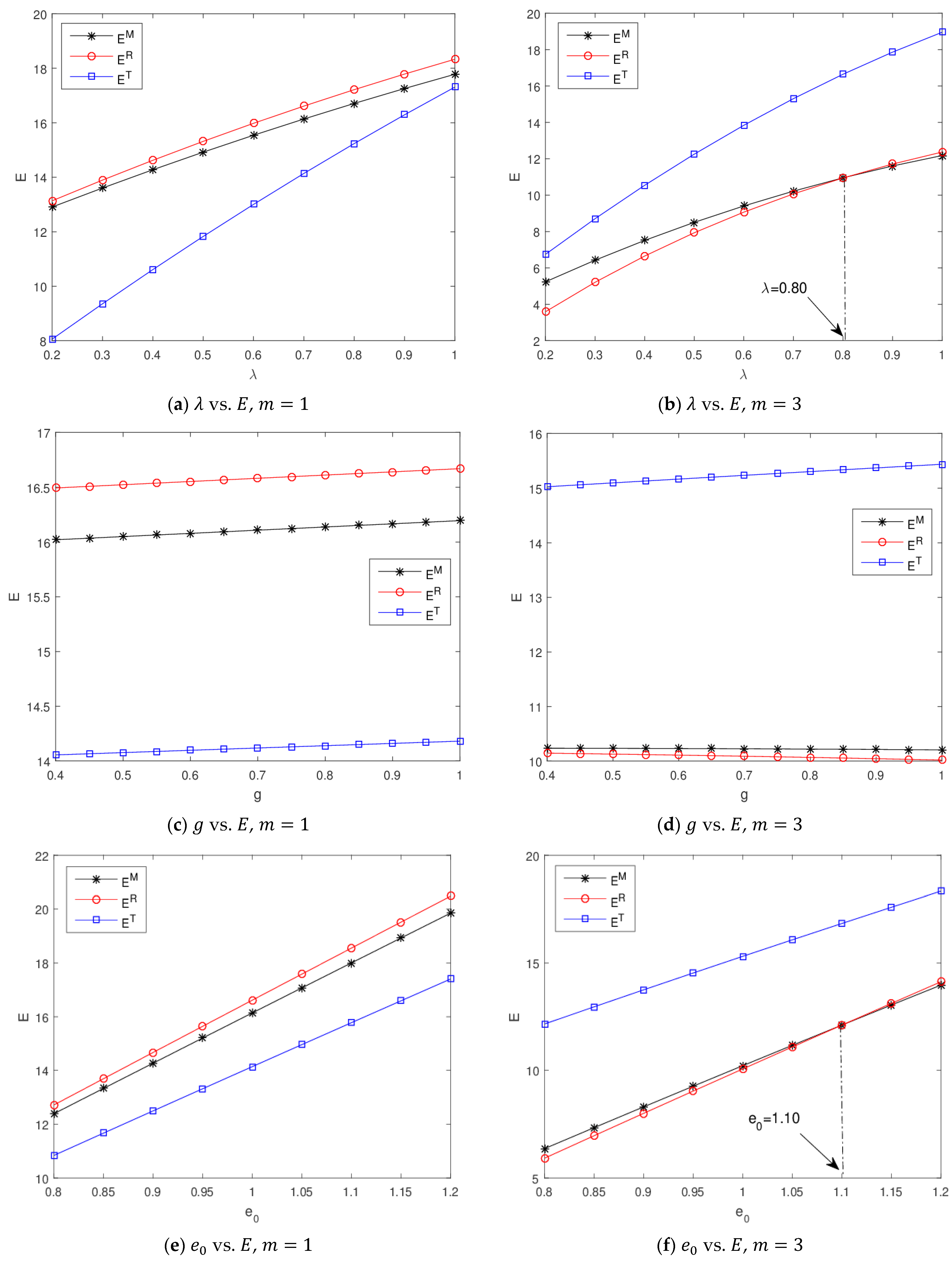
• Figure 3a,b depict the total carbon emissions and the change in the emission intensity of the remanufactured product $\lambda$. One knows that the total carbon emissions in the three Stackelberg game models increase with $\lambda$, which indicates that a large $\lambda$ is detrimental to improving the environmental benefits. The retailer-led model generates the most carbon emissions, and the third-party-led model creates the lowest carbon emissions when the carbon trading price is low, while the carbon emissions reach their maximum value in the third-party-led model when the carbon trading price is large, and the retailer-led model yields the lowest carbon emissions when $\lambda <0.8$. Otherwise, the manufacturer-led model is the most effective in enhancing environmental performance compared with other models.
• Figure 3c,d illustrates the total carbon emissions with the change in the carbon quota of a unit product $g$. When the carbon trading price is smaller, a greater $g$ corresponds to higher total carbon emissions, which implies that the loose carbon regulation is detrimental to curbing carbon emissions in such a situation. However, the carbon emissions in the third-party-led model increase with $g$, while the carbon emissions in the manufacturer-led and retailer-led models decrease with $g$. Also, the retailer-led model always generates lower carbon emissions than other models. Therefore, the retailer-led model is the best option for the closed-loop supply chain when the carbon price is high from the perspective of environmental protection.
• In observing Figure 3e,f, it becomes evident that the total carbon emissions increase with the original carbon emissions per unit product $e_0$ in different game models, i.e., the larger $e_0 \mathrm{i}\mathrm{s}$, the more total carbon emissions are generated in the production process. Moreover, the third-party-led model yields the lowest carbon emissions when the carbon trading price is low $\left(m=1\right),$while a high carbon trading price $\left(m=3\right)$leads to the third-party-led model creating the most carbon emissions.
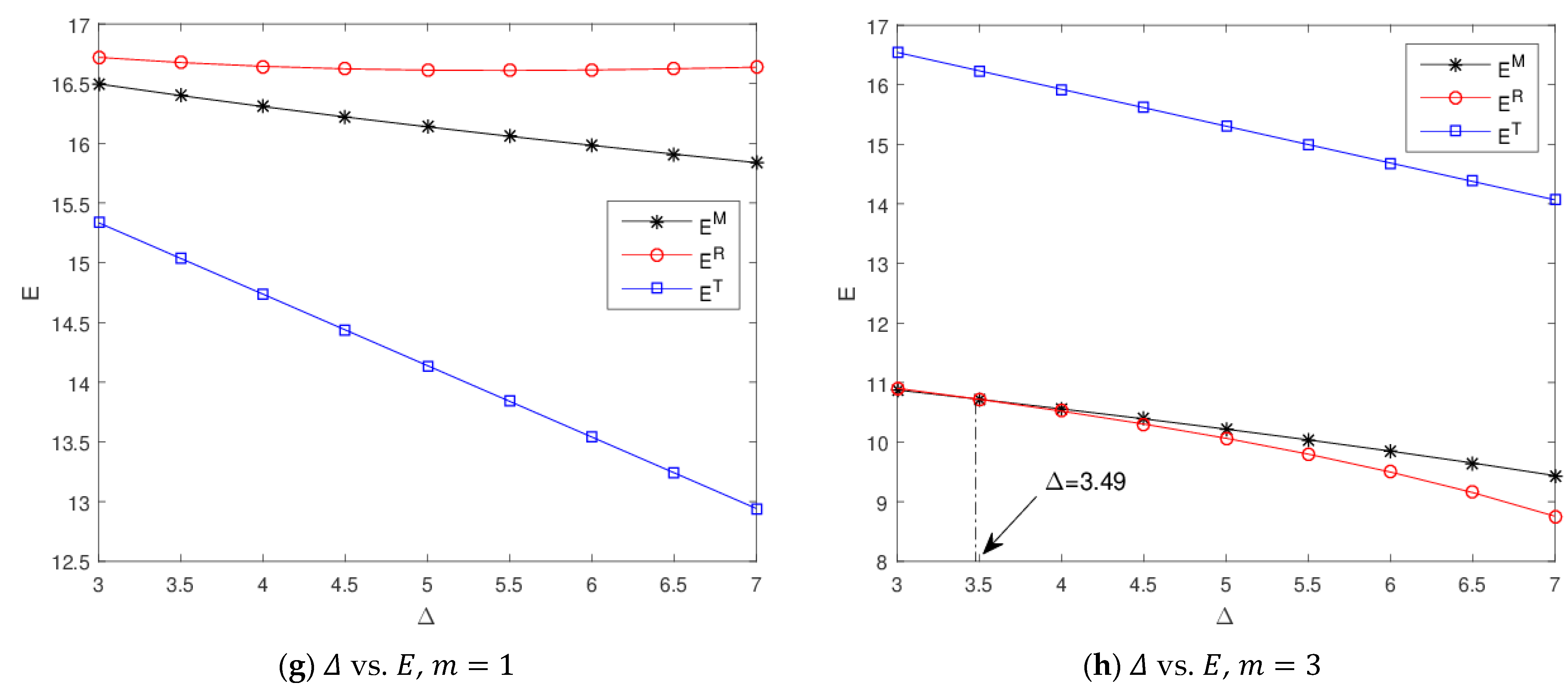
• Figure 3g,h presents the variation trend of the total carbon emissions with respect to the net production cost savings from remanufacturing $∆$ in different game models. When the carbon price is low enough, the carbon emissions of the manufacturer-led and the third-party-led models are reduced significantly, but the total carbon emissions have a slight variation, with $∆$ increasing in the retailer-led model. This demonstrates that the large ∆ can cause the manufacturer to pursue a higher emission reduction rate; thereby, the total carbon emissions are decreased. In addition, the third-party-led model achieves the greatest total carbon emissions, while the retailer-led model obtains the lowest total carbon emissions when $∆$ exceeds a certain threshold $\left(∆>3.49\right),$ in addition to the greater carbon trading price.

5.3. Impacts of Key Parameters on Profit of CLSC

In this subsection, we concentrate on investigating the joint effects of key parameters on the profits of three Stackelberg game models. Note that the original values taken for the model parameters are $\Delta =5$, $\lambda =0.7$, $g=0.8$, $k=150$, and $e_0=1$. For convenience in the analysis, we no longer consider the unit of the model parameters. Note that the values of key parameters remain unchanged when studying the simultaneous effects of the other two parameters.

Some observations are derived by conducting several numerical experiments, which are shown as follows:

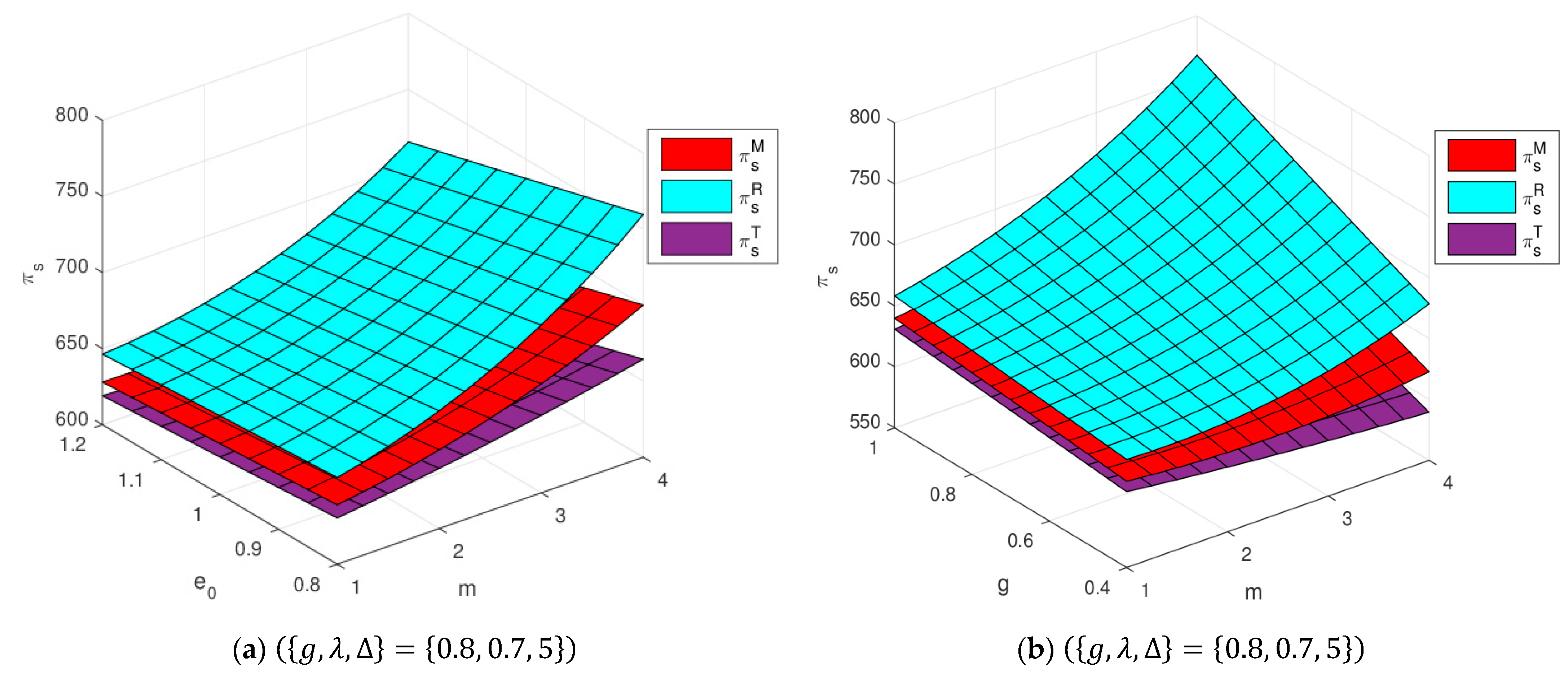
• Figure 4 is proposed to study the joint effects of the two parameters on the total profits of three different game models. One can observe that the total profits in the retailer-led model are always greater than those in other models, and the third-party-led model gains the lowest profits, which indicates the third-party-led model is least preferred from the perspective of economic performance.
• The profit levels of the three game models are improved significantly with varying values of $m,$ and their profit variations are not obvious with respect to $e_0$, as shown in Figure 4a. The greater $g$ is beneficial to enhancing the profits of the entire closed-loop supply chain, and the larger $m$ is conducive to improving the economic performance for the manufacturer-led and retailer-led models, but it leads to a profit reduction for the third-party-led model, as shown in Figure 4b. By observing Figure 4c, one can see that the relatively low $\lambda$ combined with the relatively high $\Delta$ is always conducive to elevating total profits for three game models. Moreover, Figure 4d shows that the total profits in three Stackelberg game models are reduced simultaneously, which is associated with the higher values of $\lambda$ and $k$.

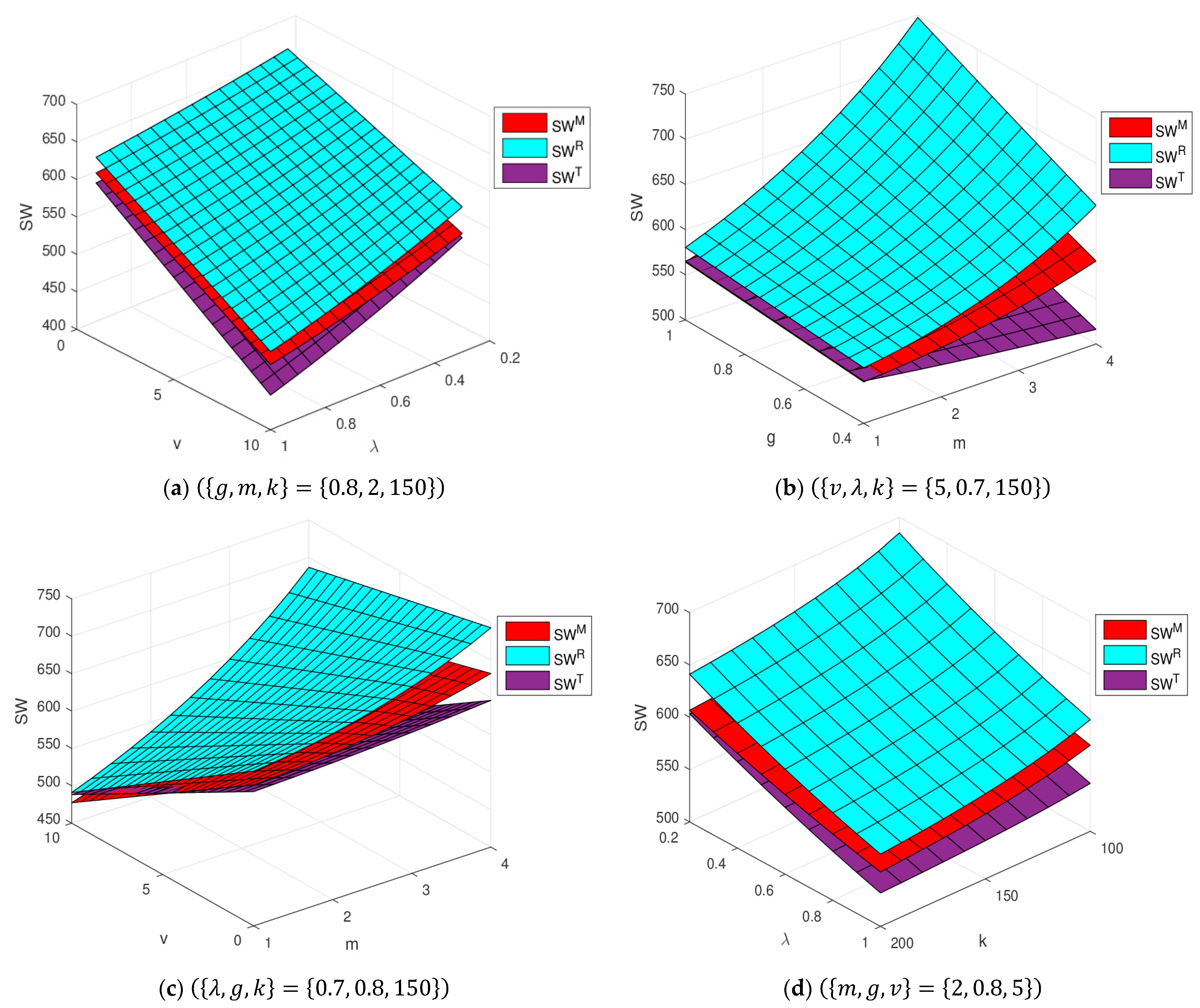
5.4. Impacts of Key Parameters on Social Welfare of CLSC

In this section, we want to explore the impacts of key parameters on the social welfare of three Stackelberg game models by performing several numerical experiments. In line with prior research [3,51], the social welfare function of the closed-loop supply chain can be formulated as follows:

$${SW}^j={\pi }_s^j+{CS}^j-v{E}^j$$

(14)

where $v$ reflects the environmental damage coefficient of the carbon emissions, which translates the emissions into monetary units. In equation (14), the first term denotes the total profits of the closed-loop supply chain; the second term indicates the consumer surplus, which is expressed as ${CS}^j=D^2/2\beta$ [3]; and the third term represents the negative impact of carbon emissions on the environment.

Figure 5 shows a comparison of the social welfare levels in three Stackelberg game models under the cap-and-trade regulation. It is apparent that the large environmental damage coefficient $\nu$ causes the social welfare of the CLSC to tolerate more losses. Therefore, the large values of $v$ and $\lambda$ are a disadvantage to improving social welfare levels, as displayed in Figure 5a. In Figure 5b, we know that the retailer-led model is the best option to obtain more social welfare for the closed-loop supply chain. Furthermore, when the value of $v$ is greater than a certain threshold and the carbon trading price $m$ is small enough, the social welfare levels in the third-party-led model are higher than that in the retailer-led model; otherwise, the third-party-led model is always the worst situation in terms of social welfare.

The joint effects of $g$ and $m$ on the social welfare of the closed-loop supply chain are shown in Figure 5c. One can see that the social welfare levels are the highest in the retailer-led model, while the lowest social welfare levels appear in the third-party-led model when the carbon trading price is relatively larger, regardless of the change of $g$. However, the manufacturer-led model generates the least social welfare when the carbon trading price is small enough. In addition, it is obvious that the smaller values of $\lambda$ and $k$ act as an advantage in terms of increasing the social welfare for the three Stackelberg game models, as shown in Figure 5d.

According to the above analysis, we can conclude that the relationships of social welfare in different game models are closely related to the carbon trading price and the environmental damage coefficient. Moreover, the retailer-led model is always the best choice for the CLSC from the perspective of social welfare.

6. Conclusions, Managerial Implications, and Future Research Directions

In the present paper, we investigate a three-level CLSC comprising a manufacturer, a retailer, and a third-party collector considering the effects of different channel power structures and cap-and-trade regulation. Three different game models are established via Stackelberg game theory, and their optimal equilibrium outcomes are obtained through the backward induction approach. We focus on exploring the joint impacts of carbon-related and remanufacturing-related parameters on optimal solutions, total carbon emissions, supply chain profits, and social welfare under different scenarios. We compare the optimum solutions and performances of channel members in the three Stackelberg game models. Furthermore, several numerical experiments are conducted to identify the best choices for the CLSC in terms of environmental and social performance under various parameter conditions. Several interesting analytical results are derived.

6.1. Findings

• Under the cap-and-trade regulation, the highest/lowest optimal wholesale and retail prices are generated in the third-party-led/retailer-led model. Moreover, a looser cap-and-trade policy and the greater net production cost savings from remanufacturing correspond to a lower wholesale and retail price, respectively, whereas the larger values of initial carbon emissions per unit product, the emission intensity of the remanufactured product, and the emission reduction cost coefficient correspond to a higher wholesale and retail price, respectively.
• The optimal transfer payment is relative to the initial carbon emissions per unit of product, the net production cost savings of remanufacturing, and the carbon emission cost savings per unit of the remanufactured product. Furthermore, the optimal transfer price in the third-party-led model is higher than those in the manufacturer-led and retailer-led models.
• The return rate consistently reaches the highest level in the third-party-led model, while the return rate of the manufacturer-led model is the lowest. Moreover, which model can achieve the emission reduction rate and return rate depends on parameter conditions.
• The carbon trading price significantly impacts optimal solutions, environmental and economic benefits, as well as social welfare. A larger carbon trading price stimulates the manufacturer to make more of an effort to reduce carbon emissions. Moreover, the emission reduction rate and profits of channel members are positive correlated with the carbon trading price in the retailer-led and third-party-led models, while they are negatively correlated with the carbon trading price in the manufacturer-led model.
• The retailer-led model is the best option for the CLSC capturing more economic benefits. Whoever undertakes the leader role will obtain the highest profit levels among three Stackelberg game models, so each channel member is driven to play the leader role in the CLSC.
• The retailer-led model always creates the most social welfare compared with the other two game models. In addition, when the carbon trading price exceeds a certain threshold, the social welfare level in the manufacturer-led model is higher than that of the third party-led model.

6.2. Managerial Implications

• Remanufacturing and green investment are beneficial to curbing carbon emissions. To encourage enterprises to actively build reverse supply chains and invest in low-carbon technologies, the government should provide financial subsidies to the enterprises, which can accelerate the creation of the green production system and a low-carbon circular economy.
• A loose cap-and-trade regulation is conducive to improving the greenness of products and the recovery rate of end-of-life products, as well as elevating the overall profit of the CLSC. Therefore, at the beginning of the carbon emission reduction project, the carbon emission credits issued by government departments should not be too low, which is conducive to the enterprises making more efforts in green investment and remanufacturing.
• Under different channel power structures, the carbon trading price has different effects on the carbon emission reduction rate and the manufacturers’ profit. To promote manufacturers to reduce carbon emissions and operational costs, it is essential for government departments to regulate carbon trading prices to some extent, thereby improving the operational efficiency of the CLSC.

6.3. Research Limitations and Future Research Directions

Indeed, our work still has some research limitations and can be extended in the following directions. First, the demand function used in our work is a deterministic function that does not consider random factors, so future research can develop a mathematical model that incorporates uncertainty scenarios related to market demand, remanufacturing and production costs, etc. Second, we assume that new and remanufactured products are indistinguishable in the consumer market. However, in reality, consumers’ willingness to pay for the new and remanufactured products is different in most cases; therefore, investigating the optimal decisions with two types of products competing in the same market is an interesting topic. Third, green products may attract more consumers with low-carbon preferences, while the proposed game model does not consider the consumers’ purchase behavior, so integrating the consumers’ low-carbon preference into the Stackelberg game model of the CLSC is a future study direction. Lastly, the channel members in the CLSC usually exhibit social preferences behaviors, such as risk aversion and fairness concern, and tend to act as bounded rational agents, so it is essential to incorporate those operational behavior factors into CLSC game models in future studies.

References

1. Yang, M. Green investment and e-commerce sales mode selection strategies with cap-and-trade regulation. Comput. Ind. Eng. 2023, 177, 109036. [Google Scholar] [CrossRef]
2. Lyu, R.; Zhang, C.; Li, Z.; Li, Y. Manufacturers’ integrated strategies for emission reduction and recycling: The role of government regulations. Comput. Ind. Eng. 2021, 163, 107769. [Google Scholar] [CrossRef]
3. Ghashghaei, M.; Golpîra, H. Optimal integration of electricity supply chain and sustainable closed-loop supply chain. Expert Syst. Appl. 2024, 241, 122464. [Google Scholar] [CrossRef]
4. Zhu, C.; Ma, J. Dynamic strategies of horizontal low-carbon supply chains under double carbon policies: A bounded rationality perspective. Comput. Ind. Eng. 2023, 181, 109309. [Google Scholar] [CrossRef]
5. Xu, S.; Govindan, K.; Wang, W.; Yang, W. Supply chain management under cap-and-trade regulation: A literature review and research opportunities. Int. J. Prod. Econ. 2024, 271, 109199. [Google Scholar] [CrossRef]
6. Fang, H.; Yu, L.; Zhang, Z. Promoting consumer returns in closed-loop supply chains under cap-and-trade regulation: A cooperative recycling advertising perspective. J. Clean. Prod. 2024, 436, 140584. [Google Scholar] [CrossRef]
7. Li, J.; Lai, K.K.; Li, Y.M. Remanufacturing and low-carbon investment strategies in a closed-loop supply chain under multiple carbon policies. Int. J. Logist. Res. App. 2022, 27, 170–192. [Google Scholar] [CrossRef]
8. Kou, X.; Liu, H.; Liu, H.; Yu, X. Cooperative emission reduction in the supply chain: The value of green marketing under different power structures. Environ. Sci. Pollut. Res. 2022, 29, 68396–68409. [Google Scholar] [CrossRef]
9. Wang, Y.; Wang, D.; Cheng, T.; Zhou, R.; Gao, J. Decision and coordination of E-commerce closed-loop supply chain chains with fairness concern. Transp. Res. Part E Logist. Transp. Rev. 2023, 173, 103092. [Google Scholar] [CrossRef]
10. Sabbaghnia, A.; Heydari, J.; Uelkue, M.A.; Zolfaghari, S. Sustainable supply chain coordination: Extant literature, trends, and future research directions. Ann. Oper. Res. 2024, 05852. [Google Scholar] [CrossRef]
11. Mondal, C.; Giri, B.C. Retailers’ competition and cooperation in a closed-loop green supply chain under governmental intervention and cap-and-trade policy. Oper. Res. 2022, 22, 859–894. [Google Scholar] [CrossRef]
12. Zhang, X.; Li, Q.; Liu, Z.; Chang, C. Optimal pricing and remanufacturing mode in a closed-loop supply chain of WEEE under government fund policy. Comput. Ind. Eng. 2021, 151, 106951. [Google Scholar] [CrossRef]
13. Yang, L.; Hu, Y.; Huang, L. Collecting mode selection in a remanufacturing supply chain under cap-and-trade regulation. Eur. J. Oper. Res. 2020, 287, 480–496. [Google Scholar] [CrossRef]
14. Cheng, P.; Ji, G.; Zhang, G.; Shi, Y. A closed-loop supply chain network considering consumer’s low carbon preference and carbon tax under the cap-and-trade regulation. Sustain. Prod. Consump. 2022, 29, 614–635. [Google Scholar] [CrossRef]
15. Wang, J.; He, S. Government interventions in closed-loop supply chains with modularity design. Int. J. Prod. Econ. 2023, 264, 108965. [Google Scholar] [CrossRef]
16. Savaskan, R.C.; Bhattacharya, S.; Van Wassenhove, L.N. Closed-loop supply chain models with product remanufacturing. Manag. Sci. 2004, 50, 239–252. [Google Scholar] [CrossRef]
17. Dou, G.; Choi, T. Does implementing trade-in and green technology together benefit the environment? Eur. J. Oper. Res. 2021, 295, 517–533. [Google Scholar] [CrossRef]
18. Guo, Y.; Wang, M.; Yang, F. Joint emission reduction strategy considering channel inconvenience under different recycling structures. Comput. Ind. Eng. 2022, 169, 108159. [Google Scholar] [CrossRef]
19. Wang, Z.; Wu, Q. Carbon emission reduction and product collection decisions in the closed-loop supply chain with cap-and-trade regulation. Int. J. Prod. Res. 2020, 59, 4359–4383. [Google Scholar] [CrossRef]
20. Hu, X.; Yang, Z.; Sun, J.; Zhang, Y. Carbon tax or cap-and-trade: Which is more viable for Chinese remanufacturing industry? J. Clean. Prod. 2019, 243, 118606. [Google Scholar] [CrossRef]
21. Zheng, B.; Jin, L.; Huang, G.; Chu, J. Retailer’s optimal CSR investment in closed-loop supply chains: The impacts of supply chain structure and channel power structure. 4OR 2023, 21, 301–327. [Google Scholar] [CrossRef]
22. Gao, J.; Han, H.; Hou, L.; Wang, H. Pricing and effort decisions in a closed-loop supply chain under different channel power structures. J. Clean. Prod. 2016, 112, 2043–2057. [Google Scholar] [CrossRef]
23. Maiti, T.; Giri, B.C. Two-way product recovery in a closed-loop supply chain with variable markup under price and quality dependent demand. Int. J. Prod. Econ. 2017, 183, 259–272. [Google Scholar] [CrossRef]
24. Ranjbar, Y.; Sahebi, H.; Ashayeri, J.; Teymouri, A. A competitive dual recycling channel in a three-level closed loop supply chain under different power structures: Pricing and collecting decisions. J. Clean. Prod. 2020, 272, 122623. [Google Scholar] [CrossRef]
25. Zhou, Y.; Zhang, Y.; Wahab, M.I.M.; Goh, M. Channel leadership and performance for a closed-loop supply chain considering competition. Transp. Res. Part E Logist. Transp. Rev. 2023, 175, 103151. [Google Scholar] [CrossRef]
26. Zhang, C.; Li, H.; Tian, Y.X. Manufacturer’s carbon abatement strategy and selection of spent power battery collecting mode based on echelon utilization and cap-and-trade policy. Comput. Ind. Eng. 2023, 177, 109079. [Google Scholar] [CrossRef]
27. Yang, L.; Wang, G.; Ke, C. Remanufacturing and promotion in dual-channel supply chains under cap-and-trade regulation. J. Clean. Prod. 2018, 204, 939–957. [Google Scholar] [CrossRef]
28. Chai, Q.; Sun, M.; Lai, K.; Xiao, Z. The effects of government subsidies and environmental regulation on remanufacturing. Comput. Ind. Eng. 2023, 178, 109126. [Google Scholar] [CrossRef]
29. Liu, Z.; Chen, J.; Diallo, C. Optimal production and pricing strategies for a remanufacturing firm. Int. J. Prod. Econ. 2018, 204, 290–315. [Google Scholar] [CrossRef]
30. Tang, S.; Wang, W.; Zhou, G. Remanufacturing in a competitive market: A closed-loop supply chain in a Stackelberg game framework. Expert Syst. Appl. 2020, 161, 113655. [Google Scholar] [CrossRef]
31. Zhang, C.; Lyu, R.; Li, Z.; MacMillen, S.J. Who should lead raw materials collection considering regulatory pressure and technological innovation? J. Clean. Prod. 2021, 298, 126762. [Google Scholar] [CrossRef]
32. Wan, N. Impacts of sales mode and recycling mode on a closed-loop supply chain. Int. J. Syst. Sci. Oper. Logist. 2023, 10, 2221076. [Google Scholar] [CrossRef]
33. Choi, T.; Li, Y.; Xu, L. Channel leadership, performance and coordination in closed loop supply chains. Int. J. Prod. Econ. 2013, 146, 371–380. [Google Scholar] [CrossRef]
34. Wang, W.; Zhang, Y.; Zhang, K.; Bai, T.; Shang, J. Reward-penalty mechanism for closed-loop supply chains under responsibility-sharing and different power structures. Int. J. Prod. Econ. 2015, 170, 178–190. [Google Scholar] [CrossRef]
35. Taleizadeh, A.A.; Sadeghi, R. Pricing strategies in the competitive reverse supply chains with traditional and e-channels: A game theoretic approach. Int. J. Prod. Econ. 2019, 215, 48–60. [Google Scholar] [CrossRef]
36. Liu, W.; Qin, D.; Shen, N.; Zhang, J.; Jin, M.; Xie, N.; Chen, J.; Chang, X. Optimal pricing for a multi-echelon closed loop supply chain with different power structures and product dual differences. J. Clean. Prod. 2020, 257, 120281. [Google Scholar] [CrossRef]
37. Zheng, B.; Yang, C.; Yang, J.; Zhang, M. Dual-channel closed loop supply chains: Forward channel competition, power structures and coordination. Inter. J. Prod. R. 2017, 55, 3510–3527. [Google Scholar] [CrossRef]
38. Wang, Q.; Chen, K.B.; Wang, S.B.; Liu, W.J. Channel structures and information value in a closed-loop supply chain with corporate social responsibility based on the third-party collection. Appl. Math. Model. 2022, 106, 482–506. [Google Scholar] [CrossRef]
39. Suvadarshini, P.; Biswas, I.; Srivastava, S. Impact of reverse channel competition, individual rationality, and information asymmetry on multi-channel closed-loop supply chain design. Int. J. Prod. Econ. 2023, 259, 108818. [Google Scholar] [CrossRef]
40. Ding, J.; Chen, W.; Wang, W. Production and carbon emission reduction decisions for remanufacturing firms under carbon tax and take-back legislation. Comput. Ind. Eng. 2020, 143, 106419. [Google Scholar] [CrossRef]
41. Wang, Q.; Xiu Xu, S.; Ji, X.; Zhao, N. Joint decisions on selling mode choice and emission reduction investment under cap-and-trade regulation. Int. J. Prod. Res. 2023, 62, 6753–6780. [Google Scholar] [CrossRef]
42. Yang, Y.; Goodarzi, S.; Bozorgi, A.; Fahimnia, B. Carbon cap-and-trade schemes in closed-loop supply chains: Why firms do not comply? Transp. Res. Part E Logist. Transp. Rev. 2021, 156, 102486. [Google Scholar] [CrossRef]
43. Lin, Y.; Yu, Z.; Wang, Y.; Goh, M. Performance evaluation of regulatory schemes for retired electric vehicle battery recycling within dual-recycle channels. J. Environ. Manag. 2023, 332, 117354. [Google Scholar] [CrossRef]
44. Ghosh, S.K.; Seikh, M.R.; Chakrabortty, M. Analyzing a stochastic dual-channel supply chain under consumers’ low carbon preferences and cap-and-trade regulation. Comput. Ind. Eng. 2020, 149, 106765. [Google Scholar] [CrossRef]
45. Narang, P.; Kanti De, P.; Peng Lim, C.; Kumari, M. Optimal recycling model selection in a closed-loop supply chain for electric vehicle batteries under carbon cap-trade and reward-penalty policies using the Stackelberg game. Comput. Ind. Eng. 2024, 196, 110512. [Google Scholar] [CrossRef]
46. Xu, J.; Jia, R.; Wang, B.; Xu, A.; Zhu, X. The optimal emission reduction and recycling strategies in construction material supply chain under carbon cap–trade mechanism. Sustainability 2023, 15, 9181. [Google Scholar] [CrossRef]
47. Chen, C.K.; Ulya, M.A. Analyses of the reward-penalty mechanism in green closed-loop supply chains with product remanufacturing. Int. J. Prod. Econ. 2019, 210, 211–223. [Google Scholar] [CrossRef]
48. Reong, S.; Chen, J.-M.; Yu, J.C.-P.; Hsiao, Y.-L.; Wee, H.-M. Optimal inbound/outbound pricing model for remanufacturing in a closed-loop supply chain. Int. J. Ind. Eng. 2022, 29, 8309. [Google Scholar]
49. Li, Z.; Pan, Y.; Yang, W.; Ma, J.; Zhou, M. Effects of government subsidies on green technology investment and green marketing coordination of supply chain under the cap-and-trade mechanism. Energ. Econ. 2021, 101, 105426. [Google Scholar] [CrossRef]
50. Zhang, Y.; Zhang, T. Complex dynamics of a low-carbon supply chain with government green subsidies and carbon cap-and-trade policies. Int. J. Bifurcat. Chaos 2022, 32, 2250090. [Google Scholar] [CrossRef]
51. Yenipazarli, A. Managing new and remanufactured products to mitigate environmental damage under emissions regulation. Eur. J. Oper. Res. 2016, 249, 117–130. [Google Scholar] [CrossRef]
52. Zhang, Y.; Zhang, T. Dynamic analysis of a dual-channel closed-loop supply chain with fairness concerns under carbon tax regulation. Environ. Sci. Pollut. Res. 2022, 29, 57543–57565. [Google Scholar] [CrossRef] [PubMed]
53. Tontini, G.; Söilen, K.S.; Zanchett, R. Nonlinear antecedents of customer satisfaction and loyalty in third-party logistics services (3PL). Asia Pac. J. Mark. Logist. 2017, 29, 1116–1135. [Google Scholar] [CrossRef]
Figure 1. The CLSC framework.
Sustainability 17 01042 g001
Figure 2. Impact of carbon trading price.
Sustainability 17 01042 g002aSustainability 17 01042 g002b
Figure 3. The influences of key parameters on total carbon emissions.
Sustainability 17 01042 g003aSustainability 17 01042 g003b
Figure 4. Influences of key parameters on the channel members’ profits.
Sustainability 17 01042 g004aSustainability 17 01042 g004b
Figure 5. Influences of key parameters on social welfare.
Sustainability 17 01042 g005