Prediction and Analysis of Spatiotemporal Evolution Trends of Water Quality in Lake Chaohu Based on the WOA-Informer Model

Abstract

Lakes, as key freshwater reserves and ecosystem cores, supply human water, regulate climate, sustain biodiversity, and are vital for global ecological balance and human sustainability. Lake Chaohu, as a crucial ecological barrier in the middle and lower reaches of the Yangtze River, faces significant environmental challenges to regional sustainable development due to water quality deterioration and consequent eutrophication issues. To address the limitations of conventional monitoring techniques, including insufficient spatiotemporal coverage and high operational costs in lake water quality assessment, this study proposes an enhanced Informer model optimized by the Whale Optimization Algorithm (WOA) for predictive analysis of concentration trends of key water quality parameters—dissolved oxygen (DO), permanganate index (CODMn), total phosphorus (TP), and total nitrogen (TN)—across multiple time horizons (4 h, 12 h, 24 h, 48 h, and 72 h). The results demonstrate that the WOA-optimized Informer model (WOA-Informer) significantly improves long-term water quality prediction performance. Comparative evaluation shows that the WOA-Informer model achieves average reductions of 9.45%, 8.76%, 7.79%, 8.54%, and 11.80% in RMSE metrics for 4 h, 12 h, 24 h, 48 h, and 72 h prediction windows, respectively, along with average improvements of 3.80%, 5.99%, 11.23%, 17.37%, and 23.26% in R² values. The performance advantages become increasingly pronounced with extended prediction durations, conclusively validating the model’s superior capability in mitigating error accumulation effects and enhancing long-term prediction stability. Spatial visualization through Kriging interpolation confirms strong consistency between predicted and measured values for all parameters (DO, CODMn, TP, and TN) across all time horizons, both in concentration levels and spatial distribution patterns, thereby verifying the accuracy and reliability of the WOA-Informer model. This study successfully enhances water quality prediction precision through model optimization, providing robust technical support for water environment management and decision-making processes.

1. Introduction

“Humans dwell by water, and civilizations thrive with water” [1]. As a critical natural resource sustaining Earth’s ecosystem balance and human societal development, freshwater protection against pollution carries significant strategic importance [2]. In recent years, rapid socioeconomic development and population growth have led to massive industrial and agricultural wastewater discharge into rivers, ultimately flowing into lakes and causing severe water pollution [3]. For instance, the Caspian Sea, a vital global water body whose water volume accounts for approximately 40% of the total water volume of the world’s lakes, exhibits distinct differentiation in its aquatic trophic status—the proportions of oligotrophic, mesotrophic, and eutrophic states are 66%, 20%, and 13%, respectively. Moreover, the current eutrophication process is continuing to advance, with the eutrophic state showing a growing trend [4]. In water pollution monitoring, the concentration of water quality factors serves as the core indicator. Constructing prediction models for major pollutant concentrations to accurately capture early signs of dynamic changes in lake water quality provides a basis for relevant authorities to respond in a timely manner, thereby safeguarding drinking water safety and maintaining ecosystem health. Water quality prediction is a key focus of water environment research and also an important foundation for water resource management and pollution prevention and control [5,6].

Advancements in data acquisition and computing performance have made data-driven machine learning methods highly advantageous in water quality simulation. Compared to traditional mechanistic models relying on linear computations via differential equation solving, machine learning, with its superior data processing and fitting capabilities, more flexibly constructs models to predict complex water quality changes [7,8,9]. For example: Wei Liu et al. established a MIC-SVR model to effectively estimate DO concentrations in the Tanjiang River, providing accurate predictions for water environment protection and resource management decisions [10]; Aggarwal Mohit et al. used response surface methodology with AdaBoost and XGBoost to evaluate interactions between TOC, NH₄⁺, TN, and PO₄³⁻ and their treatment impacts, enhancing prediction reliability through cross-validation with RSM [11]; Chen Yasong et al. developed three machine learning models to predict NH₄⁺, COD, SMX, and heavy metals in constructed wetland effluents, demonstrating that integrating scientific data analysis with machine learning supports practical engineering [12]; Mao Tianyu et al. combined multispectral imaging with BP neural networks for CODMn measurement, offering high speed, resolution, and reagent-free operation [13]; Lu Hao et al. improved lake TN/TP temporal prediction by incorporating internal nutrient loading into machine learning algorithms [14]; Li Lucen et al. used LSTM to predict organic/inorganic oxidizable pollutants, guiding targeted water quality improvement [15]; Hongyu Zuo et al. proposed the VMD-TCN-ARIMA model, reducing DO prediction RMSE by 41.05% and computation time by 26.06% [16]; Tong An et al. enhanced LSTM with feature adaptive weighting and long-term memory focusing (DA-LSTM), improving accuracy and generalization [17]; Bi Jing et al. developed the VBAED hybrid model by fusing VMD, bidirectional input Attention, BiLSTM encoder/decoder, and bidirectional temporal attention, validated as superior for water quality prediction [18]; Chen Zhanfeng et al. constructed a Bi-LSTM model with dual temporal and feature attention, achieving excellent performance in predicting water quality at 8 Pearl River estuaries and providing a new technical path for high-precision prediction under complex hydrodynamics [19].

Based on the aforementioned research status and gaps, this study takes Chaohu Lake as the research area, focuses on four core water quality parameters, namely dissolved oxygen (DO), permanganate index (CODMn), total phosphorus (TP), and total nitrogen (TN), and proposes the use of the Whale Optimization Algorithm (WOA) to optimize the hyperparameters of the Informer model, thereby developing the WOA-Informer model. The specific research objectives are as follows: (1) utilize the WOA-Informer model to achieve accurate prediction of the concentration evolution trends of Chaohu Lake’s core water quality parameters (DO, CODMn, TP, TN) over five future time horizons, 4 h, 12 h, 24 h, 48 h, and 72 h, and (2) visualize the prediction results of the WOA-Informer model using the Kriging interpolation method to intuitively present the concentration and spatial distribution evolution processes of Chaohu Lake’s water quality parameters over different prediction time horizons, verify the consistency between the model’s prediction results and the measured values, and confirm the model’s accuracy and reliability. This study aims to provide effective technical support for water environment management and decision-making in the Chaohu Lake Basin, assist in the early warning of eutrophication and pollution prevention and control in Chaohu Lake, and promote the improvement of regional aquatic ecological environment quality and sustainable development.

2. Materials and Methods

2.1. Overview of the Research Area

Lake Chaohu is situated between 117°25′–117°58′ E longitude and 31°16′–31°32′ N latitude in the central part of Anhui Province. The topography of the Lake Chaohu basin is higher in the west and lower in the east. The lakebed elevation generally ranges from 5 to 6 m, with an average water depth of 2.65 m and a maximum depth of 6.78 m. The area around Chaohu Lake is located at the junction of the two major paraplatforms (tectonic plates) of the Sino-Korean and Yangtze, with a landform pattern of being surrounded by mountains on three sides and adjacent to the lake on one side. The total population of its basin was approximately 10.6 million in 2024. The lake covers an area of approximately 780 km², with a corresponding storage capacity of about 2 BCM. It serves as a crucial drinking water source for Hefei and Chaohu cities [20,21]. As one of China’s five largest freshwater lakes, Lake Chaohu is located in the middle and lower reaches of the Yangtze River, connecting the Yangtze and Huaihe rivers, and serves as a vital channel for the Yangtze-to-Huaihe Water Diversion Project. The lake receives water from about 33 tributaries, with nine major inflow and outflow rivers, including the Nanfei River, Shiwuli River, Pai River, Hangbu River, Zhegao River, Shuangqiao River, Zhao River, Baishitian River, and Yuxi River [22].

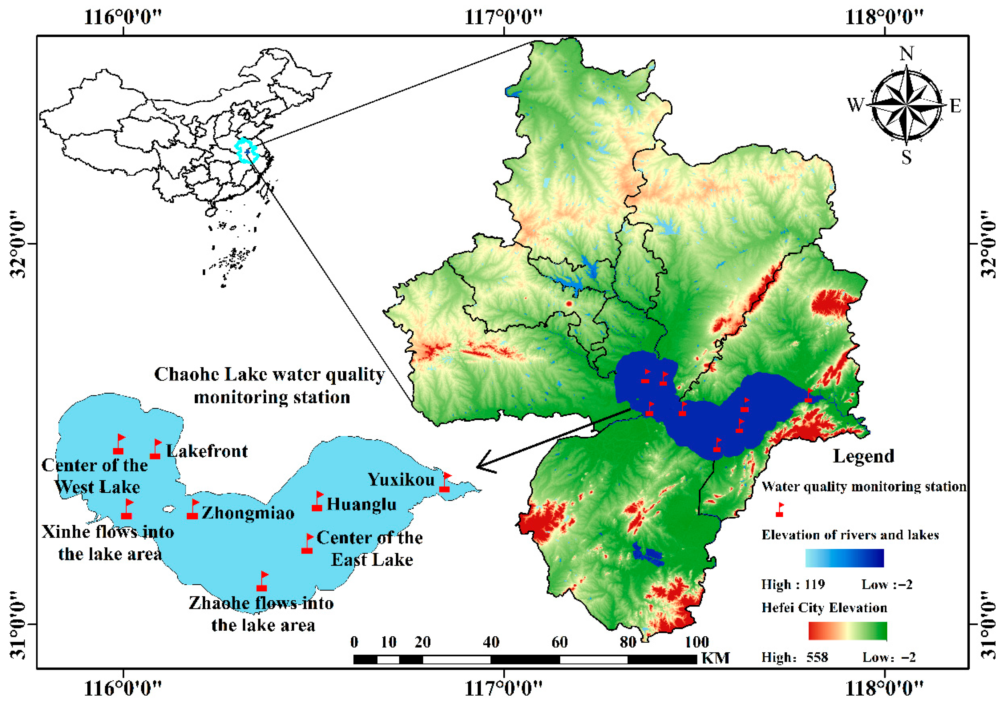
Over the past three decades, rapid population growth and industrial/agricultural development in the Lake Chaohu basin have caused a massive discharge of wastewater, elevated nutrient and organic matter concentrations, and an accelerated eutrophication process in the lake [23,24]. According to recent monitoring data, Lake Chaohu’s water quality has consistently remained at Class IV (based on China’s water quality standards), with total phosphorus (TP) being the primary pollutant. Significant amounts of nitrogen- and phosphorus-laden wastewater are discharged into the lake annually, compounded by agricultural non-point source pollution. These factors have caused severe eutrophication, leading to recurrent algal blooms (cyanobacterial blooms), which deplete dissolved oxygen (DO), harm aquatic life, and elevate the permanganate index (CODMn). Consequently, the overall water quality of Lake Chaohu continues to deteriorate [25,26,27]. Given these challenges, predicting the spatiotemporal trends of Lake Chaohu’s water quality parameters can provide early warnings and support effective water quality management. The spatial distribution of the study area, Chaohu Lake, and its water quality monitoring stations is shown in Figure 1.

2.2. Data Analysis

The study area is Lake Chaohu, and the water quality monitoring data were obtained from the National Surface Water Quality Automatic Monitoring Real-time Data Release Platform (https://szzdjc.cnemc.cn:8070/GJZ/Business/Publish/Main.html, accessed on 15 April 2025). Water quality monitoring data from 2021 to 2024 were selected as the research dataset. The water quality data from each monitoring station were recorded every 4 h, with 6 measurements per day. The collected water quality parameters include: Water temperature (°C), pH, Dissolved oxygen (DO, mg/L), Permanganate index (CODMn, mg/L), Ammonia nitrogen (NH₃-N, mg/L), Total phosphorus (TP, mg/L), Total nitrogen (TN, mg/L), Electrical conductivity (EC, μs/cm), Turbidity (NTU), Chlorophyll-a (Chl, mg/L), Algal density (Cell/L). The information on the water quality monitoring stations in Lake Chaohu used in this study is presented in

Table 1. Water quality monitoring station information of Lake Chaohu.

Number	Cross-Section Name	Longitude	Latitude
1	East Lake Center	117.6200	31.5220
2	Hubin	117.4203	31.6461
3	Huanglu	117.6331	31.5778
4	West Lake Center	117.3725	31.6527
5	Xinhe Inflow Zone	117.3832	31.5674
6	Yuxikou	117.8008	31.6025
7	Zhaohe Inflow Zone	117.5605	31.4726
8	Zhongmiao	117.4696	31.5674

.

2.3. Data Processing

During long-term monitoring, limitations in sensor network stability and climatic factors may lead to abnormal or missing water quality data due to equipment failures, network disruptions, and river drying. Additionally, environmental noise reduces the accuracy of water quality data [28]. To ensure the effective application of monitoring data in this study, systematic processing of missing values and outliers is required to guarantee data completeness and reliability.

2.3.1. Handling of Missing Values

Missing data may lead to decreased stability of prediction models and reduced reliability of results, so missing data need to be imputed [29]. Missing values can be categorized into three types: missing completely at random (MCAR), missing at random (MAR), and missing not at random (MNAR). Corresponding imputation methods should be adopted for different types of missing values [30].

In this study, Little’s Test of Missing Completely at Random (Little’s MCAR) was used to determine the type of missing water quality data. The null hypothesis (H₀) of this test is that the data are missing completely at random (MCAR), meaning that the occurrence of missing values is unrelated to other observed or unobserved values; the alternative hypothesis (H₁) is that the data are not missing completely at random (non-MCAR). The p-value is calculated via the chi-square distribution. If the p-value is greater than the set significance level (usually set at 0.05), H₀ is accepted (i.e., the data are MCAR); otherwise, H₀ is rejected [31]. Little’s MCAR test results for each water quality monitoring station are shown in

Table 2. Results of Little’s MCAR Test for Data from Each Water Quality Monitoring Point.

Monitoring Site	Chi-Square Value	Degrees of Freedom	p-Value	Null Hypothesis Holds
East Lake Center	0.0186	83,568	1.0	H0
Hubin	0.0125	92,460	1.0	H0
Huanglu	0.0154	87,552	1.0	H0
West Lake Center	0.0112	89,268	1.0	H0
Xinhe Inflow Zone	0.009	90,192	1.0	H0
Yuxikou	0.1170	100,440	1.0	H0
Zhaohe Inflow Zone	0.0187	88,356	1.0	H0
Zhongmiao	0.0094	98,304	1.0	H0

.

According to the results of Little’s MCAR test in Table 2,

Table 3. Basic information of water quality parameter data.

Monitoring Site	Water Quality Parameters	Max	Min	Mean	Standard Deviation	Variance	Median
East Lake Center	DO	14.5280	5.0720	9.6817	1.9475	3.7927	9.4760
	CODMn	6.4835	1.9097	4.1495	0.8164	0.6665	4.0590
	TP	0.1512	0.0050	0.0673	0.0286	0.0008	0.0609
	TN	2.5530	0.0500	1.1670	0.5038	0.2538	1.0800
Hubin	DO	14.9881	4.5951	9.7906	2.0757	4.3083	9.6970
	CODMn	7.4463	1.8251	4.5568	1.0059	1.0118	4.3635
	TP	0.2296	0.0245	0.0950	0.0445	0.0020	0.0826
	TN	3.1040	0.2080	1.6426	0.5506	0.3032	1.6360
Huanglu	DO	15.3556	5.0230	10.1327	2.0809	4.3302	9.9345
	CODMn	5.9420	1.8885	3.8083	0.8077	0.6524	3.6810
	TP	0.1144	0.0050	0.0588	0.0215	0.0005	0.0562
	TN	3.2527	0.0510	1.2494	0.7850	0.6162	1.0160
West Lake Center	DO	14.9370	4.2710	9.5889	2.1603	4.6667	9.4970
	CODMn	7.2879	2.4020	4.8132	0.9273	0.8600	4.6883
	TP	0.2524	0.0050	0.1095	0.0523	0.0027	0.0956
	TN	4.0203	0.2560	2.1340	0.7544	0.5692	2.0728
Xinhe Inflow Zone	DO	14.8680	3.9940	9.4349	2.1778	4.7428	9.3620
	CODMn	7.7930	2.0690	4.8698	1.0718	1.1486	4.8190
	TP	0.2142	0.0050	0.0992	0.0426	0.0018	0.0891
	TN	3.3120	0.0820	1.6253	0.6259	0.3917	1.5033
Yuxikou	DO	12.4800	2.9900	7.9578	1.9872	3.9490	7.9024
	CODMn	5.1080	0.5690	2.8265	0.9108	0.8296	2.8490
	TP	0.1145	0.0359	0.0749	0.0156	0.0002	0.0743
	TN	2.7573	0.6445	1.6972	0.4174	0.1742	1.6587
Zhaohe Inflow Zone	DO	15.1200	4.4600	9.7573	2.1448	4.6002	9.6500
	CODMn	7.5680	1.6040	4.5030	1.1751	1.3810	4.2240
	TP	0.1484	0.0050	0.0699	0.0290	0.0008	0.0653
	TN	3.2242	0.0500	1.5771	0.6112	0.3736	1.5466
Zhongmiao	DO	14.6350	4.5930	9.5966	2.0447	4.1810	9.4290
	CODMn	6.5650	1.9467	4.2201	0.8764	0.7681	4.0462
	TP	0.1865	0.0050	0.0839	0.0388	0.0015	0.0764
	TN	2.7820	0.2680	1.5193	0.5007	0.2507	1.5210

,

Table 4. Formulas of Evaluation Indicators.

Evaluation Indicators	Formula	Optimal Value
RMSE	$RMSE=\sqrt{{\displaystyle \frac{1}{n}}{\displaystyle \sum _{i=1}^n{\left(y_i-{\widehat{y}}_i\right)}^2}}$	0
R2	$R^2=1-{\displaystyle \frac{{\displaystyle {\sum }_{i=1}^n{\left({\widehat{y}}_i-y_i\right)}^2}}{{\displaystyle {\sum }_{i=1}^n{\left(y_i-\overline{y}\right)}^2}}}$	1

and

Table 5. Optimal Parameter Settings for Manual Parameter Tuning of the Informer Model.

Number	Model Parameters	Parameter Settings
1	Input duration	24 h, 72, 144 h, 192 h, 240 h
2	Predicted duration	4 h, 12 h, 24 h, 48 h, 72 h
3	e_layers	2
4	d_layers	1
5	d_model	512
6	s_layers	2
7	n_heads	8
8	d_ff	2048
9	learning_rate	0.0001
10	batch_size	32
11	train_epochs	6

, a p-Value > 0.5 indicates that the data satisfies the MCAR assumption (H₀), meaning the missing data is completely random. Given the large dataset from each monitoring station and the inherently nonlinear nature of the data, this study employs cubic spline interpolation to fill missing values in the water quality time series data [32].

Cubic spline interpolation is a method that uses piecewise third-order polynomial functions to estimate missing values. It ensures smoothness and continuity at the nodes by fitting the missing data with cubic polynomial functions within each interval. The specific computational formula is as follows.

$$S_i\left(x\right)=y_i+b_i\left(x-x_i\right)+c_i{\left(x-x_i\right)}^2+d_i{\left(x-x_i\right)}^3$$

(1)

$$b_i={\displaystyle \frac{y_{i+1}-y_i}{h_i}}-{\displaystyle \frac{h_i}{3}}\left(2M_i+M_{i+1}\right)$$

(2)

$$c_i=M_i,d_i={\displaystyle \frac{M_{i+1}-M_i}{3h_i}}$$

(3)

where $x$ and $x_i$ are the positions of the data points; $y_i$ is the function value at the data point; $h_i$ is the length of the interval; $b_i$ is the linear coefficient; $c_i$ is the quadratic coefficient; $d_i$ is the cubic coefficient; and $M_i$ and $M_{i+1}$ are the second-order derivative values.

2.3.2. Handling of Outliers

Currently, in time series tasks, outliers are commonly present in actually collected data [33]. During the monitoring process, water quality data are susceptible to isolated anomalies, periodic anomalies, and abrupt anomalies due to environmental mutations, device failures, transmission interference, etc. [34]. The 3σ criterion, as an outlier detection method, has high practicality in processing a large number of outliers in time series data and is widely used by numerous scholars. It can effectively identify and eliminate abnormal data points that do not conform to data patterns, thereby improving the accuracy and reliability of data analysis [35].

The 3σ criterion is widely applied in time series outlier processing due to its strong practicality. It calculates the mean (μ) and standard deviation (σ) of the data, and defines data beyond the range [μ − 3σ, μ + 3σ] as outliers. According to statistical principles, approximately 99% of the data should fall within this interval. Figure 2 shows the outlier detection results of water quality parameters (DO, CODMn, TP, TN) at the monitoring station in the center of the eastern half of the lake. In the figure, “Upper Limit” represents the upper limit of the water quality data (i.e., μ + 3σ), “Lower Limit” represents the lower limit (i.e., μ − 3σ), “Mean Value” is the data mean, and “Origin Data” is the actually monitored water quality data values; data outside the range of upper and lower limits in the figure are identified as outliers and require further processing.

Outliers in data can interfere with the model training process and prediction results, thus requiring outlier identification and replacement before model training, which helps improve the model’s generalization ability and the accuracy of current water quality analysis. As shown in Figure 2, data points of each water quality indicator that fall outside the interval [μ − 3σ, μ + 3σ] are identified as outliers and require targeted handling. To avoid the reoccurrence of outliers during processing, replacement is performed using the average of 200 data points before and after the outlier. This method can avoid the recurrence of outliers to the greatest extent while retaining the trend characteristics and overall fluctuation patterns of the data, thereby reducing the negative impact of data on model training and learning. The results of outlier replacement for water quality parameters (DO, CODMn, TP, TN) at the monitoring station at the center of the eastern half-lake are shown in Figure 3.

2.3.3. Normalization Processing

To avoid interference with model prediction results caused by differences in units and value ranges among various water quality indicators, normalization is required. This process retains all features, converts data into a dimensionless form within the 0–1 range, unifies statistical distributions, enables data comparability, and improves the accuracy and stability of the model [36]. Basic information on water quality parameters is shown in Table 3. To facilitate direct comparison between predicted results and measured values, denormalization of the predicted data is necessary to maintain a consistent scale with the measured data, supporting subsequent direct analysis of water quality health status. The formulas for normalization and denormalization are shown in (4) and (5), respectively.

$$X_{norm}={\displaystyle \frac{X-X_{\min }}{X_{\max }-X_{\min }}}$$

(4)

$$X=X_{norm}·\left(X_{\max }-X_{\min }\right)+X_{\min }$$

(5)

where $X$ is the original data, $X_{\min }$ and $X_{\max }$ are the minimum and maximum values of the data, respectively. The normalized data $X_{norm}$ falls within the range [0, 1].

3. Research Methods

3.1. Informer Model

The Informer model is a lightweight improvement of the traditional Transformer, designed to address issues such as complex architecture, redundant self-attention blocks, high computational load, and slow output speed. By introducing a sparsification mechanism, a distillation mechanism, and a generative decoder, the model significantly improves prediction accuracy and shortens prediction time. In 2021, scholars proposing this Transformer-based optimized algorithm [37], which achieved three major breakthroughs: proposing a probabilistic sparse self-attention mechanism, introducing a self-attention distillation method, and adopting a generative decoder to optimize the prediction process. The improved Informer is more capable of capturing input-output correlations in long sequence processing, and its structure is shown in Figure 4.

(1)

Embedding layer: An innovative input representation strategy is designed for long sequence prediction, integrating local timestamps, scalar projections, and global timestamps. This breaks through the limitations of traditional attention mechanisms in mining global information and capturing long-term dependencies, enhancing the performance of extracting long-distance dependencies.

(2)

Encoder layer: The encoder layer is composed of multiple stacked Informer blocks. Each Informer block contains two main components: a self-attention mechanism and a distillation operation.

①. The multi-head probabilistic sparse self-attention mechanism based on K-L divergence reduces memory consumption and computational costs by analyzing the long-tailed distribution of self-attention scores, using K-L divergence to identify distribution differences in the query matrix Q, and screening key queries. Its calculation formula is shown in (6).

$$KL\left(q\parallel p\right)=\ln {\displaystyle {\sum }_{l=1}^{L_K}{e}^{q_i{k}_l^T/\sqrt{d}}}-{\displaystyle \frac{1}{L_K}}{\displaystyle {\sum }_{j=1}^{L_K}{q}_i}{k}_j^T/\sqrt{d}-\ln L_K$$

(6)

To estimate the distance between the query matrix Q and a uniform distribution, the Informer model employs U-dot product evaluation, proposing an approximation method to identify the sparsity characteristics of Q and reduce computational complexity. This method computes attention scores based on top-u values and sets a sampling parameter u. The corresponding calculation formula is shown in Equation (7).

$$A\left(Q,K,V\right)=Soft\max ({\displaystyle \frac{\overline{Q}{K}^T}{\sqrt{d}}})V$$

(7)

where $\overline{Q}$ denotes the selectively extracted subset of critical query matrices, K is the key matrix, V is the value matrix, and d represents the dimensionality of the Q, K, and V matrices. With these improvements, the Informer significantly enhances prediction performance and computational efficiency compared to the Transformer. Its encoder incorporates residual connection units and normalization layers, and employs a multi-head attention mechanism to capture and discriminate information from the input sequence.

②. The Informer model adopts a probabilistic sparse self-attention mechanism to handle long sequence data, and effectively captures long-range dependencies through feature distillation techniques. During the feature mapping process, the model performs hierarchical optimization, enhancing the weights of key feature vectors. Specifically, when the feature sequence is passed from layer j to layer j + 1, feature refinement is achieved via a distillation operation, as defined in Equation (8).

$$X_{j+1}^t=MaxPool(ELU(Conv1d({[X_j^t]}_{AB})))$$

(8)

(3)

Decoder layer: In constructing the decoder, researchers can choose various strategies, such as using models like fully connected layers or recurrent neural networks. However, the design of the Informer decoder often mimics the structure of the encoder to ensure functional synergy and consistency; despite structural similarities, their parameters are generally not shared, aiming to maintain the model’s flexibility and independence to better adapt to the needs of diverse prediction tasks.

3.2. Whale Optimization Algorithm (WOA)

The Whale Optimization Algorithm (WOA) is a novel intelligent optimization algorithm. By simulating individual collaboration and target tracking strategies in whale foraging, it balances global search capability and adaptability, with the algorithm being simple and efficient [38]. Its core idea derives from the simulation of whale predatory behavior, covering three stages: encirclement, attack, and prey searching, based on which an optimization model is constructed. Specifically, after humpback whales locate prey, they trap the prey by creating a spiral bubble net, attack during spiral ascent, and achieve prey searching and predation through process reduction [39]. The algorithm process can be implemented through the following steps:

(1)

Initialization of Whale Positions: Each whale is randomly initialized within a D-dimensional solution space. The position of each whale is then updated based on two distinct strategies: spiral updating and bubble-net attack updating. In the spiral updating strategy, the whale simulates local search by spiraling around the prey, mimicking the spiral movement during hunting. The corresponding update formula is given in Equation (9).

$$X_{t+1} =X_t+A·\mid C·X_{target} -X_t \mid$$

(9)

where $X_t$ represents the current position of the whale, $X_{target}$ denotes the position of the current optimal solution (the prey’s position), A is a coefficient that controls the width of the spiral, and C is a coefficient used to control the direction of the whale’s rotation around the prey. The definitions of coefficients A and C are given in Equation (10).

$$\begin{array}{l}A=2a·r-a\\ C=2·r\end{array}$$

(10)

where a decreases linearly from 2 to 0, r is a random number 0 ≤ r ≤ 1, and A controls the range of the whale’s spiral motion.

(2)

Update the whale’s position: The update rule of the Whale Optimization Algorithm is divided into two main types based on the whale’s behavior: spiral update and bubble-net update.

(3)

Spiral update: The whale moves in a spiral around the prey, simulating a local search behavior. The calculation formula for this update method is shown in Equation (11).

$$X_{t+1 }=X_t -D·\mid C·X_{target }-X_t \mid$$

(11)

where D is the distance between the whale and the target solution, defined in Equation (12).

$$D=\mid C·X_{target}-X_t\mid$$

(12)

(4)

Iterative update mechanism: The Whale Optimization Algorithm (WOA) selects behaviors based on the distance to the prey: a spiral update is used for short distances, while a bubble-net update is applied for long distances.

(5)

Termination condition: The algorithm terminates the search process based on either the maximum number of iterations or when the convergence threshold is reached.

The Whale Optimization Algorithm (WOA) demonstrates significant advantages due to its unique bionic mechanism: First, it enhances global search capabilities by simulating bubble-net behavior, effectively avoiding local optima; second, the spiral update improves local search precision; third, it has fewer control parameters (a, r), making it easier to apply to various optimization problems; fourth, it exhibits better convergence speed than traditional methods in multi-peak optimization; and fifth, its simulation of natural predation behavior gives it good adaptability, enabling it to handle multi-dimensional complex optimization problems.

3.3. Evaluation Indicators of the Model

This study uses Root Mean Square Error (RMSE), and the coefficient of determination (R²) to comprehensively evaluate the model’s performance. The formulas for each evaluation metric are shown in Table 4.

In the formula, $y_i$ represents the i-th observed value, ${\widehat{y}}_i$ represents the i-th predicted value, $n$ is the sample size, and $\overline{y}$ is the mean of the observed values.

4. Results and Analysis

4.1. Impact of Prediction Duration on Model Performance

This study uses the control variable method for model experimentation, aiming to explore the impact of model input length and prediction length on model performance. By fixing other model parameters, the input length and prediction length are adjusted separately to evaluate their effects on the prediction results. The input length, prediction length, and manually tuned optimal parameter settings for the model are shown in Table 5.

Multiple control variable experiments were conducted to investigate the impact of input length on the model. In the experiments, the input lengths were set to 24 h, 72 h, 144 h, 192 h, and 240 h, combined with prediction lengths of 4 h, 12 h, 24 h, 48 h, and 72 h. The model accuracy and runtime were compared. As shown in

Table 6. Average Prediction Accuracy for Different Prediction Steps under Different Prediction Step Lengths.

Number of Trials	Step Input Length (h)	Training Duration	Average Model Accuracy R2 (%)
1	24	1 min 27 s	44.81
2	72	2 min 6 s	51.63
3	144	2 min 39 s	63.19
4	192	4 min 57 s	63.57
5	240	7 min 32 s	64.02

, when the input length was 144 h, the model’s overall performance was the best. As the input length increased further, the improvement in model accuracy became more limited, while the training time significantly increased. Therefore, 144 h was chosen as the input length for subsequent experiments.

Through experiments on input length, it was found that when the input length was 144 h, the model exhibited excellent accuracy and runtime performance. To further investigate the impact of prediction length on model performance, a control variable experiment for prediction length was conducted. In the experiment, prediction lengths of 4 h, 12 h, 24 h, 48 h, and 72 h were used, and the results for each prediction length were compared. For the convenience of plotting, the monitoring stations of East Lake Center, Lakeshore, Huanglu, West Lake Center, Xihe Inflow Area, Yuxikou, Zhaohou Inflow Area, and Zhongmiao are represented as Site 1, Site 2, Site 3, Site 4, Site 5, Site 6, Site 7, and Site 8, respectively.

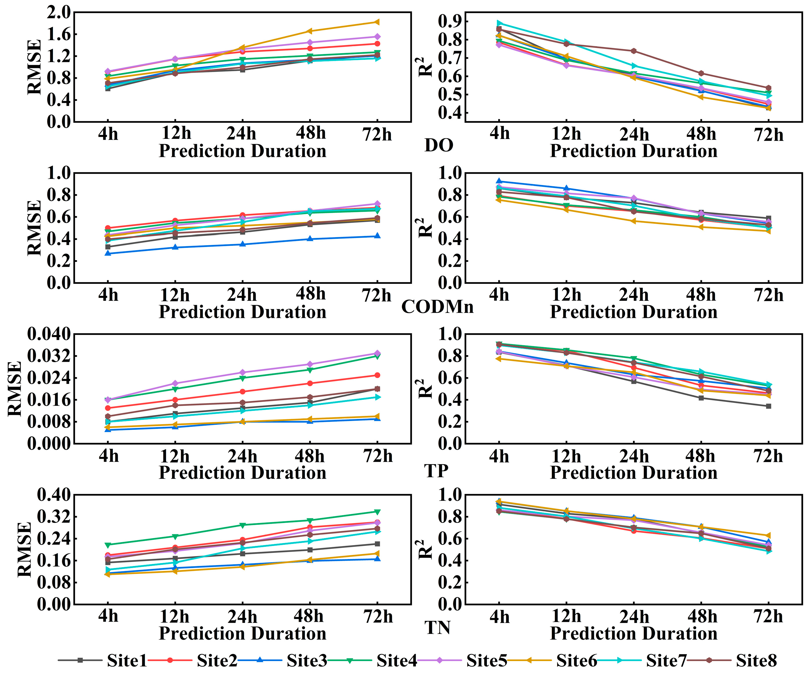
Comprehensive analysis of Figure 5 and Figure 6 reveals that the prediction performance of the Informer model for various water quality parameters at different stations decreases with the increase in prediction duration, characterized by an increase in RMSE and a decrease in R². The details are as follows:

(1)

For DO, the average RMSE is 1.105, with a maximum value of 1.822 (Station 6) and a minimum value of 0.606 (Station 1); the average R² is 0.634, with a maximum value of 0.890 (Station 7) and a minimum value of 0.426 (Station 6). As the prediction duration increases, the prediction performance of DO gradually decreases: RMSE increases from 0.606 to 1.822, with an average increase of 43.46%; R² decreases from 0.890 to 0.426, with an average decrease of 43.40%.

(2)

For CODMn, the average RMSE is 0.517, with a maximum value of 0.720 (Station 5) and a minimum value of 0.267 (Station 3); the average R² is 0.680, with a maximum value of 0.924 (Station 3) and a minimum value of 0.471 (Station 6). With the extension of prediction duration, the prediction performance of CODMn gradually declines: RMSE rises from 0.267 to 0.720, with an average increase of 34.58%; R² drops from 0.924 to 0.471, with an average decrease of 37.21%.

(3)

For TP, the average RMSE is 0.016, with a maximum value of 0.033 (Station 5) and a minimum value of 0.005 (Station 3); the average R² is 0.668, with a maximum value of 0.912 (Station 4) and a minimum value of 0.342 (Station 1). As the prediction duration increases, the prediction performance of TP gradually deteriorates: RMSE increases from 0.005 to 0.033, with an average increase of 49.61%; R² decreases from 0.912 to 0.342, with an average decrease of 45.76%.

(4)

For TN, the average RMSE is 0.206, with a maximum value of 0.339 (Station 4) and a minimum value of 0.110 (Station 6); the average R² is 0.724, with a maximum value of 0.939 (Station 6) and a minimum value of 0.486 (Station 7). With the increase in prediction duration, the prediction performance of TN gradually decreases: RMSE increases from 0.110 to 0.339, with an average increase of 39.07%; R² decreases from 0.939 to 0.486, with an average decrease of 39.54%.

Overall, in the predictions with durations of 4 h, 12 h, 24 h, 48 h, and 72 h, the model performance declines significantly with the increase in duration, with an average increase of 41.68% in RMSE and an average decrease of 41.48% in R².

Comprehensive analysis of Figure 5 and Figure 6 shows that the model maintains good prediction performance during the 4 h to 12 h period; while in the 24 h to 72 h period, due to the error accumulation effect, its performance gradually declines, with the prediction accuracy at 72 h decaying particularly significantly. At the parameter level, the prediction performance of DO and CODMn remains stable; TP and TN, however, exhibit a prominent increase in long-term prediction errors due to their high environmental sensitivity. At the station level, Stations 8 and 2 show good prediction stability, Station 5 performs the best, while Stations 1 and 3 are relatively poor. Overall, the model’s prediction performance is significantly negatively correlated with the time dimension, declining gradually as the prediction cycle extends, and the decay is more obvious under longer prediction durations. Although manual parameter tuning can slightly improve performance, it has the limitations of heavy workload and limited effectiveness.

4.2. The Impact of Optimized Algorithms on the Model

From the results in Section 4.1, it can be seen that the prediction performance of the Informer model decreases as the prediction duration increases, with a more significant decline after 48 h. Although manual parameter tuning can slightly improve performance, it has the problems of heavy workload and limited effectiveness. To avoid unreasonable parameter settings limiting model performance, the Whale Optimization Algorithm (WOA) is introduced to optimize the key hyperparameters of Informer, aiming to find optimal parameter combinations that maximize prediction capability. The parameter settings of WOA are shown in

Table 7. Parameter Settings of the Whale Optimization Algorithm.

Number	Parameters of the WOA	Setting of Numerical Values
1	hunting_party	25
2	spiral_param	1
3	mu	1
4	min_values	−100
5	max_values	100
6	iterations	500

.

In Table 7, hunting_party represents the size of the whale population (i.e., the number of solutions); spiral_param is the spiral parameter that controls the whale’s spiral movement; mu is a parameter related to the reproduction process; min_values and max_values represent the minimum and maximum values of the solution space; iterations refers to the number of iterations. The WOA is used to optimize the parameters of the Informer model, and the function accepts five parameters (X1, X2, X3, X4, X5), which represent the hyperparameters of the Informer model. Their specific roles are as follows: X1 is used to calculate d_model, controlling the model’s dimensionality; X2 is used to set dropout, which is the dropout rate applied during training to prevent overfitting; X3 is used to set d_ff, which is the hidden layer dimensionality of the feed-forward neural network; X4 is used to set e_layers, which represents the number of encoder layers; X5 is used to set d_layers, which represents the number of decoder layers.

After optimizing the hyperparameters of the Informer model using the Whale Optimization Algorithm (WOA), the best parameter configuration was obtained. After performing a global automatic search for the optimal combination of X1, X2, X3, X4, and X5 with the WOA, the water quality time-series data was predicted, and the prediction results are as follows.

Through the analysis of Figure 7 and Figure 8, the Informer model optimized by the Whale Optimization Algorithm (WOA) (WOA-Informer) has achieved significant improvements in the RMSE metrics for predicting the water quality parameters DO, CODMn, TP, and TN in Chaohu Lake. The specific performance is as follows:

In DO prediction, compared with the original Informer model, WOA-Informer reduced the RMSE by an average of 11.60% (4 h), 11.76% (12 h), 9.89% (24 h), 8.98% (48 h), and 11.07% (72 h) across Stations 1–7. The maximum reduction at each time point occurred at Station 6 (26.30% at 4 h, 33.72% at 12 h, 42.89% at 24 h, 50.24% at 48 h, 47.26% at 72 h), while the minimum reductions were concentrated at Station 5 (6.18% at 4 h, 3.74% at 12 h, 3.15% at 72 h) and Station 3 (1.77% at 48 h).

For CODMn prediction, the average RMSE reduction rates of WOA-Informer were 7.75% (4 h), 3.21% (12 h), 4.71% (24 h), 7.46% (48 h), and 9.80% (72 h). The maximum reductions were observed at Station 6 (12.68% at 4 h), Station 1 (5.49% at 12 h), and Station 5 (10.96% at 24 h, 50.24% at 48 h, 22.50% at 72 h). The minimum reductions were at Station 7 (1.55% at 4 h), Station 8 (0.66% at 12 h, 2.39% at 48 h), Stations 1–2 (1.95% at 24 h), and Station 4 (3.95% at 72 h).

In TP prediction, the average RMSE reduction rates were 12.44% (4 h), 14.97% (12 h), 10.98% (24 h), 10.01% (48 h), and 14.44% (72 h). The maximum improvements were at Station 3 (20.00% at 4 h, 25.00% at 24 h, 25.00% at 48 h), Station 8 (28.57% at 12 h), and Station 7 (17.65% at 72 h). The minimum reductions were at Stations 4–5 (6.25% at 4 h), Station 5 (4.55% at 12 h, 3.85% at 24 h, 3.45% at 48 h), and Station 6 (10.00% at 72 h).

For TN prediction, the average RMSE reduction rates were 6.01% (4 h), 5.09% (12 h), 5.57% (24 h), 7.71% (48 h), and 11.90% (72 h). The most significant improvements were at Station 1 (10.46% at 4 h) and Station 7 (12.42% at 12 h, 22.93% at 24 h, 15.15% at 48 h, 19.17% at 72 h). The minimum reductions were at Station 8 (1.82% at 4 h), Station 5 (1.54% at 12 h), Station 2 (1.27% at 24 h), Station 6 (4.29% at 48 h), and Station 3 (9.09% at 72 h).

In summary, WOA-Informer significantly improved the prediction performance of water quality parameters across different monitoring stations and prediction durations, fully verifying the effectiveness of the WOA in optimizing the overall prediction capability of the Informer model.

Analysis of Figure 9 and Figure 10 reveals that the Informer model optimized by the WOA (WOA-Informer) has significantly improved the prediction performance of Chaohu Lake’s water quality parameters (DO, CODMn, TP, and TN) in terms of the R² metric. The performance of each parameter across different stations and prediction durations is as follows:

In DO prediction, the R² values of WOA-Informer showed an average increase of 4.51%, 8.81%, 14.10%, 16.08%, and 23.52% in the 4 h, 12 h, 24 h, 48 h, and 72 h predictions at Stations 1–7, respectively. Specifically, the R² (4 h) at Station 1 increased from 0.860 to 0.875, and the R² (72 h) significantly improved from 0.427 to 0.572; the R² (72 h) at Stations 2 and 7 increased by 25.96% (0.447→0.563) and 21.6% (0.494→0.601), respectively; the R² (4 h) at Station 6 rose from 0.822 to 0.924, with the 72 h R² increasing by 12.42%.

For CODMn prediction, the R² of WOA-Informer increased by an average of 6.56% (4 h), 7.27% (12 h), 13.17% (24 h), 17.93% (48 h), and 18.22% (72 h) under the same stations and durations. The maximum increase at each duration occurred at Station 6 (15.78% at 4 h, 22.74% at 12 h, 36.83% at 24 h, 37.67% at 48 h, 28.24% at 72 h); the minimum increases were concentrated at Station 3 (0.54% at 4 h), Station 5 (0.009% at 12 h, 1.95% at 24 h, 9.39% at 72 h), and Station 1 (6.40% at 48 h).

In TP prediction, the R² of WOA-Informer increased by an average of 2.23% (4 h), 5.57% (12 h), 12.91% (24 h), 27.82% (48 h), and 30.12% (72 h). The maximum increases at each duration were observed at Station 6 (8.39% at 4 h, 10.45% at 12 h) and Station 1 (29.58% at 24 h, 57.07% at 48 h, 58.19% at 72 h); the minimum increases were concentrated at Station 4 (0.44% at 4 h, 2.69% at 24 h), Station 2 (0.47% at 12 h), and Station 7 (3.80% at 48 h, 8.52% at 72 h).

For TN prediction, the R² of WOA-Informer increased by an average of 1.89%, 2.30%, 4.74%, 7.64%, and 21.17% in the 4 h, 12 h, 24 h, 48 h, and 72 h predictions at Stations 1–7, respectively. Specifically, the R² (72 h) at Station 1 increased from 0.517 to 0.681 (a 31.7% improvement); the R² (72 h) at Station 3 rose from 0.569 to 0.690 (a 21.3% increase); the R² at Station 2 showed a steady improvement with extended prediction durations (e.g., from 0.860 to 0.896, an increase of 4.19%); the R² (4 h) at Station 6 slightly increased to 0.939, with a smaller rise in long-term predictions, which may be related to the stable TN concentration at this station and its low susceptibility to external interference.

In summary, WOA-Informer significantly improved the R² values in predicting all water quality parameters, and the improvement amplitude generally increased with extended prediction durations, fully verifying the effectiveness of the WOA in optimizing model performance.

In summary, after optimizing Informer parameters via the Whale Optimization Algorithm (WOA), the WOA-Informer model maintains stable performance in short-term time series prediction and achieves significant improvements in long-term time series prediction. The prediction accuracy of dissolved oxygen (DO), permanganate index (CODMn), total phosphorus (TP), and total nitrogen (TN) has been enhanced, among which DO and TP, which exhibit strong time series variability, show the most significant improvements. For the 72 h prediction duration, the model’s R² metrics have all improved, indicating that WOA can enhance the model’s ability to extract temporal characteristics of water quality and significantly improve the prediction accuracy of long-term water quality evolution trends. Therefore, to study the future evolution trends of Chaohu Lake’s water quality parameters, the trained WOA-Informer model is used to predict the future time series of Chaohu Lake’s water quality, clarify its evolution trends, and provide a basis for formulating targeted rectification measures, controlling the concentrations of water quality parameters, and thereby improving the water quality of Chaohu Lake.

4.3. Analysis of the Actual Application Results of the WOA-Informer Model

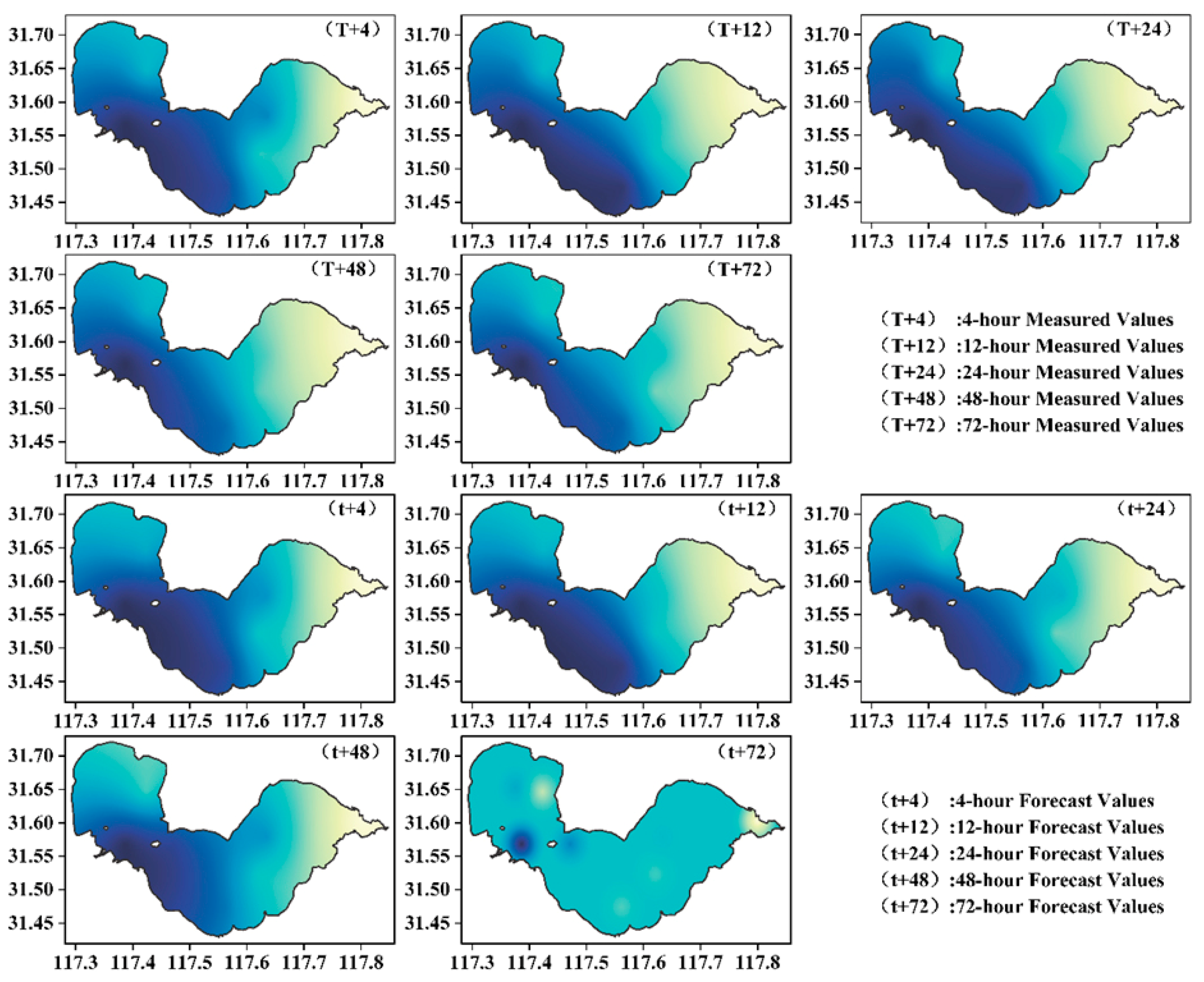
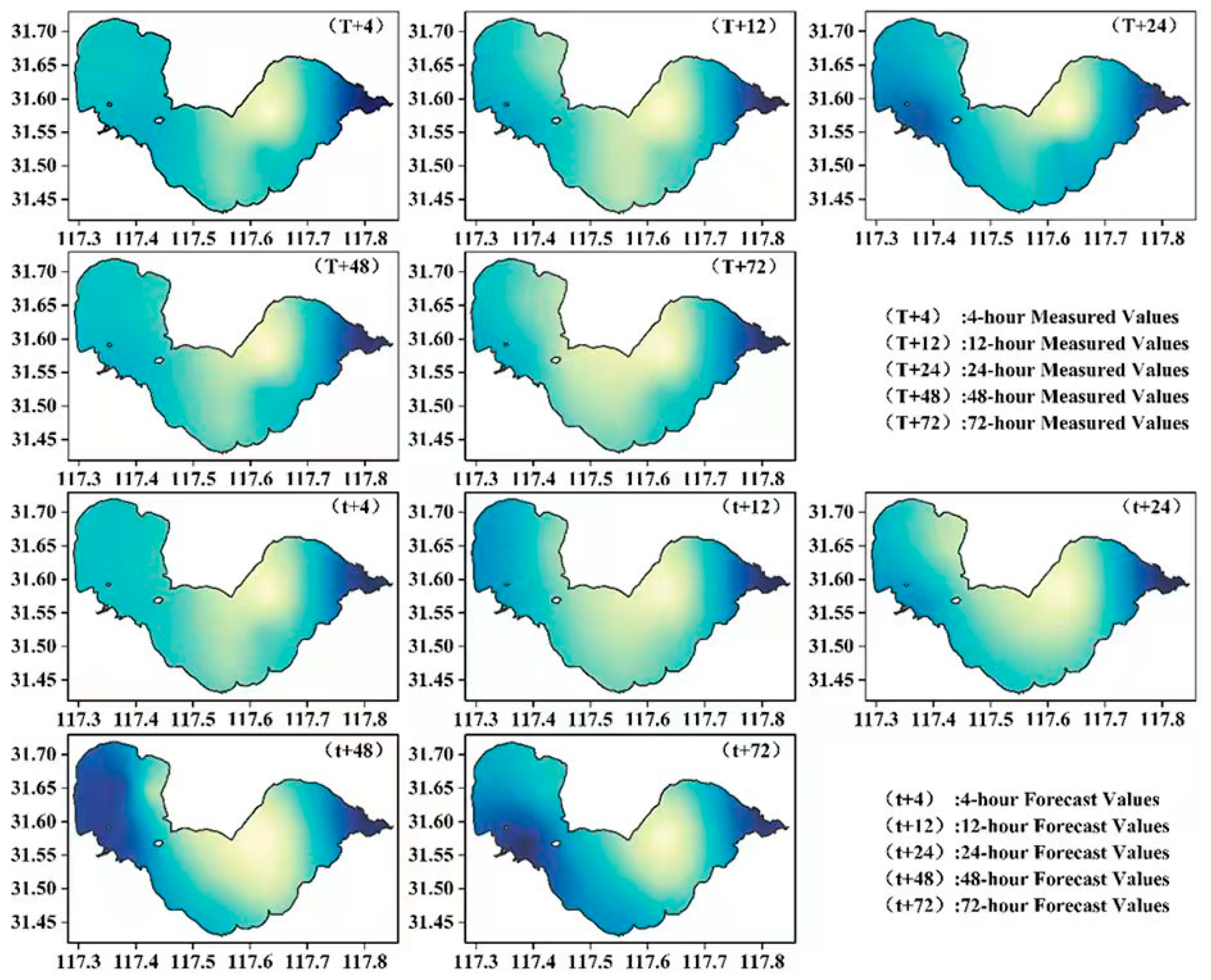
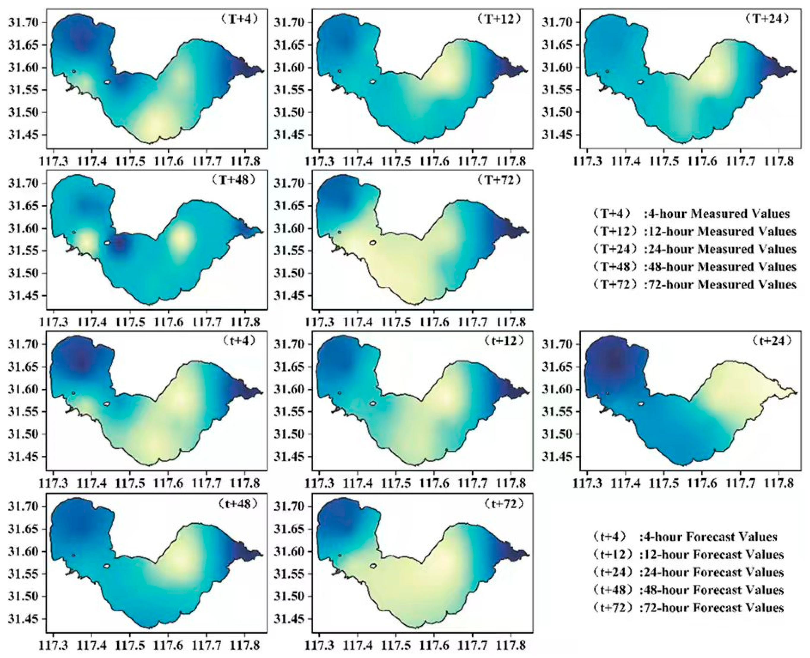
To more intuitively illustrate the concentration evolution patterns of the water quality parameters—Dissolved Oxygen (DO), Permanganate Index (CODMn), Total Phosphorus (TP), and Total Nitrogen (TN)—in Lake Chaohu over the next 4 h, 12 h, 24 h, 48 h, and 72 h, this study employs a dataset comprising 70,128 time-series samples (8766 observations per station × 8 monitoring stations), collected at 4-h intervals from 2021 to 2024. This dataset was used to train the WOA-Informer model. Based on the trained model, predictions were made for the concentrations of DO, CODMn, TP, and TN at specific future timestamps: 4:00 on 1 January 2025 (4 h ahead), 12:00 noon on 1 January (12 h ahead), 00:00 on 2 January (24 h ahead), 00:00 on 3 January (48 h ahead), and 00:00 on 4 January (72 h ahead). The predicted values for all eight monitoring stations at each timestamp were then visualized using Kriging interpolation, providing a clear depiction of the spatial distribution and temporal evolution of water quality parameters in Lake Chaohu.

4.3.1. Dissolved Oxygen (DO)

The comparison between the predicted concentrations of DO in Lake Chaohu for the future 4 h, 12 h, 24 h, 48 h, and 72 h using the WOA-Informer model and the observed values is shown in

Table 8. Comparison of Predicted and Measured Values of DO Concentration by the Mode.

Monitoring Site		Site 1	Site 2	Site 3	Site 4	Site 5	Site 6	Site 7	Site 8
4 h	T + 4	12.31	14.11	14.05	14.58	12.69	11.32	13.39	13.72
	t + 4	11.98	13.94	13.82	14.31	12.49	11.24	12.86	13.53
12 h	T + 4	12.36	14.54	13.66	14.59	12.42	11.16	13.49	12.66
	t + 4	12.06	13.88	13.35	13.99	12.18	11.28	12.73	12.64
24 h	T + 4	12.26	14.44	13.50	14.51	12.36	11.05	13.70	12.73
	t + 4	12.11	13.45	13.38	13.99	12.27	11.20	12.75	12.72
48 h	T + 4	12.14	14.01	13.71	15.05	12.31	11.29	13.51	12.94
	t + 4	12.18	12.79	13.18	13.46	12.08	11.21	12.37	12.62
72 h	T + 4	12.12	13.68	13.31	14.45	12.42	11.23	13.17	12.78
	t + 4	12.26	12.22	12.99	13.88	11.88	11.23	12.70	12.54

Note: T represents the actual measurement; t represents the prediction.

. It can be concluded that for the t + 4 prediction, the maximum error percentage is 3.9%, while the minimum error is 0.7%; for the t + 12 prediction, the maximum error percentage is 5.6%, and the minimum error is 0.2%; for the t + 24 prediction, the maximum error percentage is 10.6%, and the minimum error is 0.4%; for the t + 48 prediction, the maximum error percentage is 10.7%, and the minimum error is 0.7%; for the t + 72 prediction, the maximum error percentage is 3.9%, and the minimum error is 0.02%. This demonstrates that the WOA-Informer model also provides accurate predictions for future data. However, as the forecast horizon increases, the prediction accuracy gradually decreases.

Figure 11 presents the comparison between the observed concentrations of DO and the predicted concentrations of DO at future time points (T + 4, T + 12, T + 24, T + 48, and T + 72) based on the WOA-Informer model. From Figure 11, it can be observed that the distribution of DO at T + 4, T + 12, T + 24, T + 48, and T + 72 shows that, over time, high concentrations gradually spread from the Xinhe River inlet area towards the western and eastern lake centers. At T + 48 and T + 72, high concentrations shift from the western and eastern lake centers back towards the Xinhe River inlet area. In the WOA-Informer model’s predictions, at t + 4, t + 12, and t + 24, high concentrations of DO are mainly concentrated in the Xinhe River inlet and Zhaohua River inlet areas, with signs of spreading towards the western and eastern lake centers. At t + 48, the high-concentration DO area begins to shrink towards the Xinhe River and Zhaohua River inlet areas. However, at t + 72, it is evident that the simulation error of the WOA-Informer model increases. Overall, the predicted concentration distribution of DO at t + 4, t + 12, t + 24, t + 48, and t + 72 based on the WOA-Informer model shows a high degree of consistency with the actual DO distribution.

4.3.2. Permanganate Index (CODMn)

The comparison between the predicted concentrations of CODMn in Lake Chaohu for the future 4 h, 12 h, 24 h, 48 h, and 72 h using the WOA-Informer model and the observed values is shown in

Table 9. Comparison of Predicted and Measured Values of CODMn Concentration by the Mode.

Monitoring Site		Site 1	Site 2	Site 3	Site 4	Site 5	Site 6	Site 7	Site 8
4 h	T + 4	2.94	3.27	3.97	4.07	2.00	3.40	3.56	3.39
	t + 4	2.80	3.32	3.76	3.99	3.30	3.25	3.67	3.20
12 h	T + 4	2.79	3.27	3.50	3.68	3.02	1.57	3.89	3.01
	t + 4	2.89	3.28	3.65	3.96	3.25	3.27	3.90	3.14
24 h	T + 4	2.96	3.29	3.79	3.54	3.21	1.45	3.73	3.21
	t + 4	2.98	3.28	3.70	4.08	3.42	3.28	3.96	3.18
48 h	T + 4	2.81	3.20	3.68	3.77	3.22	3.59	3.72	3.29
	t + 4	3.15	3.30	3.78	4.27	3.55	3.33	4.09	3.29
72 h	T + 4	2.71	3.33	3.68	4.11	3.02	2.49	3.57	3.07
	t + 4	3.31	3.31	3.86	4.45	3.67	3.37	4.02	3.35

Note: T represents the actual measurement; t represents the prediction.

. It can be concluded that for the t + 4 prediction, the maximum error percentage is 64.8% (at the Lakeside station), and the minimum error is 0.16%; for the t + 12 prediction, the maximum error percentage occurs at the Yuxikou station, with the minimum error being 0.3%; for the t + 24 prediction, the station with the maximum error percentage is also Yuxikou station, with the minimum error being 0.4%; for the t + 48 prediction, the maximum error percentage is 13.3%, and the minimum error is 0.03%; for the t + 72 prediction, the maximum error percentage is 35.3%, and the minimum error is 0.6%. Upon analyzing the stations with large errors, it is noted that the observed data used in this study were not processed. The large errors occurred at points where the observed values showed significant discrepancies from neighboring data, suggesting that there may be monitoring errors at these points.

Figure 12 shows the comparison between the observed concentrations of CODMn and the predicted concentrations of CODMn at future time points (T + 4, T + 12, T + 24, T + 48, and T + 72) based on the WOA-Informer model. From Figure 12, it can be seen that as time progresses, the concentration of CODMn gradually spreads from the Xinhe River inlet and Zhongmiao station to the surrounding areas. At T + 24, the area of high concentration distribution is the largest. Between T + 48 and T + 72, the concentration of CODMn gradually decreases, starting from the Zhaohua River inlet and spreading outward, with the high-concentration distribution area reaching its minimum at T + 72. In the WOA-Informer model’s predictions, at t + 4, the high-concentration regions are located in the Xinhe River inlet and Zhongmiao station, which is consistent with the observed values. Meanwhile, at t + 12 and t + 24, CODMn further spreads, gradually extending towards the western and eastern lake centers. At t + 48 and t + 72, the high-concentration areas gradually shrink, with the smallest high-concentration distribution area at t + 72. Overall, the predicted concentration distribution of CODMn at future time points (4 h, 12 h, 24 h, 48 h, and 72 h) based on the WOA-Informer model shows consistency with the actual distribution and evolution process of CODMn.

4.3.3. Total Phosphorus (TP)

The comparison between the predicted concentrations of TP for the future time points (T + 4, T + 12, T + 24, T + 48, and T + 72) using the WOA-Informer model and the observed values is shown in

Table 10. Comparison of Predicted and Measured Values of TP Concentration by the Mode.

Monitoring Site		Site 1	Site 2	Site 3	Site 4	Site 5	Site 6	Site 7	Site 8
4 h	T + 4	0.036	0.030	0.038	0.040	0.038	0.058	0.036	0.019
	t + 4	0.038	0.034	0.039	0.041	0.040	0.062	0.041	0.024
12 h	T + 4	0.039	0.035	0.041	0.047	0.038	0.062	0.041	0.027
	t + 4	0.040	0.040	0.040	0.049	0.041	0.067	0.049	0.029
24 h	T + 4	0.038	0.033	0.035	0.047	0.034	0.053	0.038	0.021
	t + 4	0.040	0.046	0.044	0.055	0.041	0.068	0.046	0.032
48 h	T + 4	0.038	0.031	0.036	0.041	0.035	0.060	0.037	0.019
	t + 4	0.040	0.051	0.048	0.065	0.046	0.070	0.066	0.038
72 h	T + 4	0.041	0.038	0.033	0.045	0.038	0.063	0.040	0.027
	t + 4	0.041	0.056	0.052	0.074	0.048	0.072	0.054	0.031

Note: T represents the actual measurement; t represents the prediction.

. It can be concluded that for the prediction at t + 4, the maximum error percentage is 24.6%, while the minimum error is 0.7%; for the prediction at t + 12, the maximum error percentage is 21.2%, and the minimum error is 0.2%; for the prediction at t + 24, the maximum error percentage is 55.3%, and the minimum error is 6.6%; for the prediction at t + 48, the maximum error percentage is 95.4% (Huanglu station), and the minimum error is 5.69%; for the prediction at t + 72, the maximum error percentage is 64% (Xinhe River inlet area), and the minimum error is 0.06%. After error analysis, it was found that the original observed data used in this study were not pre-processed, and some abnormal data points had significant differences from adjacent monitoring values, which could have been caused by measurement errors or equipment malfunctions.

Figure 13 shows the comparison between the observed concentrations of TP and the predicted concentrations at future time points (T + 4, T + 12, T + 24, T + 48, and T + 72) using the WOA-Informer model. From Figure 13, it can be observed that for the predictions at t + 4, t + 12, and t + 24, the model’s predicted values are highly consistent with the TP evolution characteristics reflected by the observed data. However, for the predictions at t + 48 and t + 72, there is some discrepancy between the model’s predictions and the observed TP evolution. In particular, the TP concentration distribution in the eastern half of the lake remains relatively consistent, while there is a noticeable difference between the predicted and observed values in the western half of the lake. The possible reason for this phenomenon is that the abnormal values at certain monitoring points had a significant impact on the overall distribution pattern, leading to an increase in prediction errors.

4.3.4. Total Nitrogen (TN)

The comparison between the predicted TN concentrations at future time points (T + 4, T + 12, T + 24, T + 48, and T + 72) using the WOA-Informer model and the observed values is shown in

Table 11. Comparison of Predicted and Measured Values of TN Concentration by the Mode.

Monitoring Site		Site 1	Site 2	Site 3	Site 4	Site 5	Site 6	Site 7	Site 8
4 h	T + 4	1.120	0.870	1.486	1.052	1.393	1.634	1.554	1.043
	t + 4	1.214	1.037	1.443	1.158	1.503	1.727	1.706	0.994
12 h	T + 4	1.339	1.230	1.428	1.267	1.337	2.180	1.772	0.579
	t + 4	1.326	1.139	1.426	1.369	1.433	1.986	1.737	0.968
24 h	T + 4	1.505	1.259	1.505	1.462	1.506	2.163	1.676	0.800
	t + 4	1.309	1.406	1.411	1.377	1.540	0.863	1.711	0.959
48 h	T + 4	1.218	1.261	1.664	0.965	1.436	1.574	1.459	0.946
	t + 4	1.296	1.432	1.411	1.397	1.563	1.862	1.674	0.944
72 h	T + 4	1.623	1.251	1.447	1.061	1.337	1.957	1.950	1.169
	t + 4	1.400	1.448	1.418	1.421	1.583	1.855	1.745	1.327

Note: T represents the actual measurement; t represents the prediction.

. It can be concluded that for the t + 4 prediction, the maximum error percentage is 19.2%, with the minimum error percentage being 2.9%. For the t + 12 prediction, the maximum error percentage is 67.1%, with the minimum error being 0.1%. For the t + 24 prediction, the maximum error percentage is 60.1%, with the minimum error being 2.1%. For the t + 48 prediction, the maximum error percentage is 44.7%, with the minimum error being 0.23%. For the t + 72 prediction, the maximum error percentage is 33.9%, with the minimum error being 2%. In general, as the prediction time increases, the errors fluctuate significantly. The maximum error percentage reaches its peak at the 12-h prediction, then gradually decreases, while the minimum error remains at a low level.

Figure 14 shows the comparison between the observed TN concentrations and the concentrations predicted by the WOA-Informer model for the future time points (T + 4, T + 12, T + 24, T + 48, and T + 72). From the analysis of Figure 14, it can be concluded that for the short-term predictions at t + 4 and t + 12, as well as the medium-term prediction at t + 24, the trend prediction results of the WOA-Informer model are generally consistent with the concentration changes and distribution characteristics reflected by the monitoring data. However, for the long-term predictions at t + 48 and t + 72, the prediction performance of the WOA-Informer model shows a significant decline. Specifically, the high-concentration area in the western half of the lake is systematically underestimated, and the predicted concentrations in the eastern half of the lake are overestimated. Overall, the spatial heterogeneity is reduced. A possible reason for this phenomenon is that the collected water quality monitoring data was not processed before use, and noise interference may exist.

5. Discussion

With the rapid advancement of urbanization and industrialization, water resources are increasingly threatened by severe pollution [40]. Under the active promotion of ecological environment big data construction and its application in early warning and forecasting, ecological monitoring of water resources and the prediction of water quality evolution trends have become critical research topics in the current context [41]. By monitoring and forecasting the evolution trends of water quality characteristics such as pH value, dissolved oxygen (DO), permanganate index (CODMn), ammonia nitrogen, and total phosphorus (TP), it is possible to effectively assess the degree of water pollution and issue timely warnings regarding changes in water quality [42]. This holds significant scientific and practical importance for advancing the digital management of Chaohu Lake, improving the water environment quality of the watershed, and safeguarding regional water security. Against this backdrop, this study takes the time-series water quality data from 8 monitoring stations around Chaohu Lake during 2021–2024 as the foundation, integrates the Whale Optimization Algorithm (WOA) with the Informer model to construct a WOA-Informer hybrid model. After training the model using data from 2021 to 2024, the study predicts key water quality parameters such as DO, CODMn, TP, and total nitrogen (TN) in early 2025 for forecast horizons of 4 h, 12 h, 24 h, 48 h, and 72 h. Additionally, Kriging interpolation is employed to visualize the observed and predicted spatiotemporal distributions of these parameters across the same forecast horizons. The visualization results indicate that the concentrations and distributions of DO, CODMn, TP, and TN are generally consistent within the 4 h, 12 h, and 24 h forecast horizons; while in the 48 h and 72 h forecast horizons, although there are relatively large discrepancies at some stations, the overall trends remain similar. This successfully achieves the trend prediction of DO, CODMn, TP, and TN concentrations and distributions in Chaohu Lake for the upcoming 4 h, 12 h, 24 h, 48 h, and 72 h, providing technical support for the early warning of water quality evolution.

However, there are still obvious limitations in the current field of water quality monitoring and prediction. On one hand, traditional water quality monitoring methods are restricted by insufficient spatiotemporal coverage, long time consumption, and high labor intensity, making it difficult to fully reflect changes in the water environment and future trends [43]. On the other hand, although deep learning models (such as the Informer model) are widely used in water quality prediction tasks and have advantages in handling long-sequence time-series data, the performance of such models is highly dependent on parameter settings and optimization strategies. During long-term forecasting, they are prone to error accumulation, leading to a decline in prediction accuracy and stability, which makes it difficult to meet the requirements of long-term water quality forecasting in complex and dynamic aquatic environments [44,45,46]. To address this, many researchers have attempted to combine machine learning algorithms with water quality monitoring data to achieve accurate predictions [47,48]. This study also optimizes the parameters of the Informer model by introducing WOA, constructing the WOA-Informer model, which significantly improves the long-term water quality prediction performance for Chaohu Lake. Compared with the original Informer model, the WOA-Informer model reduces the Root Mean Square Error (RMSE) by an average of 9.45%, 8.76%, 7.79%, 8.54%, and 11.80% for the 4 h, 12 h, 24 h, 48 h, and 72 h prediction tasks, respectively, and increases the coefficient of determination (R²) by an average of 3.80%, 5.99%, 11.23%, 17.37%, and 23.26%. Moreover, as the forecast horizon extends, its advantages in mitigating error accumulation and improving long-term prediction stability become more prominent [49]. Nevertheless, this optimization scheme is still only targeted at the Chaohu Lake region and has not been fully verified in other watersheds or environmental scenarios, so the generalization ability of the model needs to be further expanded.

In the future, further research can be carried out in the following directions: First, apply the WOA-Informer model to more different types of watersheds (such as rivers, reservoirs, and coastal waters), combine the water quality characteristics and environmental factors of each region to verify and optimize the model parameters, and further improve the adaptability and generalization ability of the model under complex environmental conditions, thereby providing an effective technical path for water quality prediction in other regions. Second, on the basis of the existing water quality parameter prediction, incorporate more dynamic factors affecting water quality (such as meteorological conditions, hydrological regimes, and the intensity of human activities) to construct a more comprehensive multi-factor coupled prediction model, and enhance the accuracy and foresight of water quality evolution trend prediction. Third, based on the long-term prediction advantages of the model, combine it with the ecological environment big data platform to develop an integrated water quality early warning and management system, realizing the seamless connection of water quality prediction, risk assessment, and emergency decision-making. This will provide more comprehensive theoretical and methodological support for watershed water environment governance and water security assurance, and promote the development of water quality prediction technology in a more efficient and practical direction.

6. Conclusions

To meet the long-term forecasting requirements for water quality parameters of Chaohu Lake, this study constructed an improved Informer model based on the Whale Optimization Algorithm (WOA), named WOA-Informer. Focusing on core water quality parameters including dissolved oxygen (DO), chemical oxygen demand (CODMn), total phosphorus (TP), and total nitrogen (TN), the study systematically compared and evaluated the forecasting performance of the WOA-Informer model before and after optimization by WOA under five prediction time horizons: 4 h, 12 h, 24 h, 48 h, and 72 h. On this basis, the model was further used to predict the spatiotemporal evolution patterns of Chaohu Lake’s water quality parameters within the aforementioned future time horizons. The prediction results were visualized using Kriging interpolation, and the main research conclusions were finally formulated.

(1)

The use of the WOA to adaptively optimize the Informer model significantly enhances the model’s ability to recognize complex temporal features of water quality parameters. After optimization, the model’s performance in long-term 72-h prediction tasks shows a significant reduction in Root Mean Square Error (RMSE), with the RMSE for dissolved oxygen (DO) and total phosphorus (TP) decreasing by 47.27% and 28.57%, respectively. The maximum improvement in the coefficient of determination (R²) reaches 31.7%, which fully demonstrates the superiority of the Whale Optimization Algorithm in reducing error accumulation and enhancing long-term prediction stability.

(2)

Within the short-term prediction range (4–12 h), the WOA-Informer model exhibits excellent performance, with the average R² not falling below 0.85. However, as the prediction duration increases, the model’s prediction accuracy shows a downward trend. Overall, the model improves prediction accuracy for longer time spans compared to the Informer model, especially in predicting total nitrogen (TN) and total phosphorus (TP) concentrations. The average R² for 72 h predictions decreases to 0.55 and 0.52, respectively. Additionally, in the spatial dimension, the prediction accuracy difference between Huanglu station and Yuxikou station is particularly notable, revealing the potential impacts and limitations of pollutant transport pathways and hydrological environmental factors on the model’s generalization performance.

(3)

The Kriging interpolation method is used to visualize the WOA-Informer model’s predictions of dissolved oxygen (DO), chemical oxygen demand (CODMn), total phosphorus (TP), and total nitrogen (TN) in Chaohu Lake for the next 4 h, 12 h, 24 h, 48 h, and 72 h. The predicted water quality concentration and distribution trends closely align with the actual measurements, demonstrating the accuracy and reliability of the WOA-Informer model. Additionally, using Kriging interpolation to convert the model’s prediction results into visual images provides a reliable tool for real-time water quality monitoring and pollution warning in Chaohu Lake.

References

1. Uddin, M.G.; Bamal, A.; Diganta, M.T.M.; Sajib, A.M.; Rahman, A.; Abioui, M.; Olbert, A.I. The role of optimizers in developing data-driven model for predicting lake water quality incorporating advanced water quality model. Alex. Eng. J. 2025, 122, 411–435. [Google Scholar] [CrossRef]
2. Baron, J.S.; Poff, N.L.; Angermeier, P.L.; Dahm, C.N.; Gleick, P.H.; Hairston, N.G., Jr.; Jackson, R.B.; Johnston, C.A.; Richter, B.D.; Steinman, A.D. Meeting ecological and societal needs for freshwater. Ecol. Appl. 2002, 12, 1247–1260. [Google Scholar] [CrossRef]
3. Liu, M.; Li, J.; Li, Y.; Gao, W.; Lu, J. Data-driven identification of pollution sources and water quality prediction using Apriori and LSTM models: A case study in the Hanjiang River basin. J. Contam. Hydrol. 2025, 272, 104570. [Google Scholar] [CrossRef]
4. Mozafari, Z.; Noori, R.; Siadatmousavi, S.M.; Afzalimehr, H.; Azizpour, J. Satellite-based monitoring of eutrophication in the Earth’s largest transboundary lake. GeoHealth 2023, 7, e2022GH000770. [Google Scholar] [CrossRef]
5. Noor, S.S.M.; Saad, N.A.; Akhir, M.F.M.; Rahim, M.S.A. QUAL2K Water Quality Model: A Comprehensive Review of Its Applications, and Limitations. Environ. Model. Softw. 2024, 184, 106284. [Google Scholar] [CrossRef]
6. Nong, X.; He, Y.; Chen, L.; Wei, J. Machine learning-based evolution of water quality prediction model: An integrated robust framework for comparative application on periodic return and jitter data. Environ. Pollut. 2025, 369, 125834. [Google Scholar] [CrossRef]
7. Chen, P.; Wang, B.; Wu, Y.; Wang, Q.; Huang, Z.; Wang, C. Urban river water quality monitoring based on self-optimizing machine learning method using multi-source remote sensing data. Ecol. Indic. 2023, 146, 109750. [Google Scholar] [CrossRef]
8. Liang, Y.; Ding, F.; Liu, L.; Yin, F.; Hao, M.; Kang, T.; Zhao, C.; Wang, Z.; Jiang, D. Monitoring water quality parameters in urban rivers using multi-source data and machine learning approach. J. Hydrol. 2025, 648, 132394. [Google Scholar] [CrossRef]
9. Zhong, H.; Yuan, Y.; Luo, L.; Ye, J.; Chen, M.; Zhong, C. Water quality prediction of MBR based on machine learning: A novel dataset contribution analysis method. J. Water Process Eng. 2022, 50, 103296. [Google Scholar] [CrossRef]
10. Liu, W.; Lin, S.; Li, X.; Li, W.; Deng, H.; Fang, H.; Li, W. Analysis of dissolved oxygen influencing factors and concentration prediction using input variable selection technique: A hybrid machine learning approach. J. Environ. Manag. 2024, 357, 120777. [Google Scholar] [CrossRef]
11. Mohit, A.; Remya, N. Exploring effects of carbon, nitrogen, and phosphorus on greywater treatment by polyculture microalgae using response surface methodology and machine learning. J. Environ. Manag. 2024, 356, 120728. [Google Scholar] [CrossRef]
12. Tan, X.; Bai, Y.; Yue, X.; Jia, X. A Mamba-based method for multi-feature water quality prediction fusing dual denoising and attention enhancement. J. Hydrol. 2025, 660, 133424. [Google Scholar] [CrossRef]
13. Mao, T.; Jiang, C.; Bian, H.; Meng, X.; Jiang, C.; Cai, Y. Permanganate index detection using multi-spectral images combined with BP neural network algorithm. Optik 2022, 268, 169787. [Google Scholar] [CrossRef]
14. Lu, H.; Yang, L.; Fan, Y.; Qian, X.; Liu, T. Novel simulation of aqueous total nitrogen and phosphorus concentrations in Taihu Lake with machine learning. Environ. Res. 2022, 204, 111940. [Google Scholar] [CrossRef] [PubMed]
15. Li, L. Study on dissolved oxygen, ammonia-nitrogen and permanganate index in water of Lake Dianchi. In Proceedings of the IOP Conference Series: Materials Science and Engineering, Guangzhou, China, 20–22 December 2019; Volume 806, No. 1. p. 012008. [Google Scholar]
16. Zuo, H.; Gou, X.; Wang, X.; Zhang, M. A combined model for water quality prediction based on VMD-TCN-ARIMA optimized by WSWOA. Water 2023, 15, 4227. [Google Scholar] [CrossRef]
17. An, T.; Feng, K.; Cheng, P.; Li, R.; Zhao, Z.; Xu, X.; Zhu, L. Adaptive prediction for effluent quality of wastewater treatment plant: Improvement with a dual-stage attention-based LSTM network. J. Environ. Manag. 2024, 359, 120887. [Google Scholar] [CrossRef] [PubMed]
18. Bi, J.; Chen, Z.; Yuan, H.; Zhang, J. Accurate water quality prediction with attention-based bidirectional LSTM and encoder–decoder. Expert Syst. Appl. 2024, 238, 121807. [Google Scholar] [CrossRef]
19. Ding, F.; Hao, S.; Jiang, M.; Liu, H.; Wang, J.; Hao, B.; Yuan, H.; Mao, H.; Hu, Y.; Li, W.; et al. An improved graph neural network integrating indicator attention and spatio-temporal correlation for dissolved oxygen prediction. Ecol. Inform. 2025, 87, 103126. [Google Scholar] [CrossRef]
20. Wu, L.; Liu, K.; Wang, Z.; Yang, Y.; Sang, R.; Zhu, H.; Wang, X.; Pang, Y.; Tong, J.; Liu, X.; et al. Temporal–Spatial Variations in Physicochemical Factors and Assessing Water Quality Condition in River–Lake System of Chaohu Lake Basin, China. Sustainability 2025, 17, 2182. [Google Scholar] [CrossRef]
21. Yao, S.; Zhang, Y.; Wang, P.; Xu, Z.; Wang, Y.; Zhang, Y. Long-term water quality prediction using integrated water quality indices and advanced deep learning models: A case study of Chaohu Lake, China, 2019–2022. Appl. Sci. 2022, 12, 11329. [Google Scholar] [CrossRef]
22. Gao, X.; Qian, Y.; Fang, Y.; Shi, X.; Yao, S.; Dong, B.; Ji, K.; Wang, Z. Road network expansion and landscape dynamics in the Chaohu Lake wetland: A 20-year analysis. Ecol. Indic. 2025, 173, 113443. [Google Scholar] [CrossRef]
23. Gobler, C.J.; Drinkwater, R.W.; Anthony, A.; Goleski, J.A.; Famularo-Pecora, A.M.E.; Wallace, M.K.; Straquadine, N.R.W.; Hem, R. Sewage-and fertilizer-derived nutrients alter the intensity, diversity, and toxicity of harmful cyanobacterial blooms in eutrophic lakes. Front. Microbiol. 2024, 15, 1464686. [Google Scholar] [CrossRef]
24. Luo, L.; Tan, J.; Dzakpasu, M.; Lou, C.; Guo, W.; Ngo, H.H.; Wang, X. Impact of recharge water source quality on Chlorella vulgaris growth and biomass: Strategies for eutrophication control in urban landscape lakes. Sci. Total Environ. 2024, 957, 177740. [Google Scholar] [CrossRef]
25. Wang, Z.; Sun, F.; Sang, Y.; Wu, F. Drivers analysis and future scenario-based predictions of nutrient loads in key lakes and reservoirs of the Yangtze River Catchment. J. Environ. Manag. 2025, 374, 124078. [Google Scholar] [CrossRef]
26. Sun, T.; Zhu, L.; Huang, T.; Tao, P.; Bao, Y.; Wang, B.; Sun, Q.; Chen, K. Seasonal distribution patterns of P-cycling-related microbes and its association with internal phosphorus release in the eutrophic Lake Chaohu, China. J. Environ. Sci. 2025, 154, 226–237. [Google Scholar] [CrossRef]
27. Ding, F.; Hao, S.; Zhang, W.; Jiang, M.; Chen, L.; Yuan, H.; Wang, N.; Li, W.; Xie, X. Using multiple machine learning algorithms to optimize the water quality index model and their applicability. Ecol. Indic. 2025, 172, 113299. [Google Scholar] [CrossRef]
28. Rodriguez-Perez, J.; Leigh, C.; Liquet, B.; Kermorvant, C.; Peterson, E.; Sous, D.; Mengersen, K. Detecting technical anomalies in high-frequency water-quality data using artificial neural networks. Environ. Sci. Technol. 2020, 54, 13719–13730. [Google Scholar] [CrossRef]
29. Zhang, Y.; Thorburn, P.J. Handling missing data in near real-time environmental monitoring: A system and a review of selected methods. Future Gener. Comput. Syst. 2022, 128, 63–72. [Google Scholar] [CrossRef]
30. Pham, T.M.; Pandis, N.; White, I.R. Missing data, part 2. Missing data mechanisms: Missing completely at random, missing at random, missing not at random, and why they matter. Am. J. Orthod. Dentofac. Orthop. 2022, 162, 138–139. [Google Scholar] [CrossRef] [PubMed]
31. Little, R.J. A test of missing completely at random for multivariate data with missing values. J. Am. Stat. Assoc. 1988, 83, 1198–1202. [Google Scholar] [CrossRef]
32. More, K.S.; Wolkersdorfer, C. Exploring advanced statistical data analysis techniques for interpolating missing observations and detecting anomalies in mining influenced water data. ACS EST Water 2023, 4, 1036–1045. [Google Scholar] [CrossRef]
33. Du, X.; Zuo, E.; Chu, Z.; He, Z.; Yu, J. Fluctuation-based outlier detection. Sci. Rep. 2023, 13, 2408. [Google Scholar] [CrossRef]
34. Sun, Z.; Gao, M.; Jiang, A.; Zhang, M.; Gao, Y.; Wang, G. Incomplete data processing method based on the measurement of missing rate and abnormal degree: Take the loose particle localization data set as an example. Expert Syst. Appl. 2023, 216, 119411. [Google Scholar] [CrossRef]
35. Sun, G.; Jiang, P.; Xu, H.; Yu, S.; Guo, D.; Lin, G.; Wu, H. Outlier detection and correction for monitoring data of water quality based on improved VMD and LSSVM. Complexity 2019, 2019, 9643921. [Google Scholar] [CrossRef]
36. Wang, Y.; Qu, D.; Zhao, C.; Yang, D. Study on CA-CFAR Algorithm Based on Normalization Processing of Background Noise for HI of Optical Fiber. Photonic Sens. 2018, 8, 341–350. [Google Scholar] [CrossRef]
37. Zhou, H.; Zhang, S.; Peng, J.; Zhang, S.; Li, J.; Xiong, H.; Zhang, W. Informer: Beyond efficient transformer for long sequence time-series forecasting. In Proceedings of the AAAI Conference on Artificial Intelligence, Online, 2–9 February 2021; Volume 35, No. 12. pp. 11106–11115. [Google Scholar]
38. Huang, Y.; Ngaopitakkul, A.; Yoomak, S. Charging pile fault prediction method combining whale optimization algorithm and long short-term memory network. Energy Inform. 2025, 8, 70. [Google Scholar] [CrossRef]
39. Wang, J.; Han, Y.; Wang, H.; Ding, J.; Yi, C. Prediction of rolling bearing performance degradation based on whale optimization algorithm and backpropagation model. J. Low Freq. Noise Vib. Act. Control 2025, 44, 290–301. [Google Scholar] [CrossRef]
40. Kishore, S.; Malik, S.; Shah, M.P.; Bora, J.; Chaudhary, V.; Kumar, L.; Sayyed, R.Z.; Ranjan, A. A comprehensive review on removal of pollutants from wastewater through microbial nanobiotechnology-based solutions. Biotechnol. Genet. Eng. Rev. 2024, 40, 3087–3112. [Google Scholar] [CrossRef]
41. Wang, X.; Li, Y.; Qiao, Q.; Tavares, A.; Liang, Y. Water quality prediction based on machine learning and comprehensive weighting methods. Entropy 2023, 25, 1186. [Google Scholar] [CrossRef]
42. Xu, T.; Ma, W.; Chen, J.; Duan, L.; Li, H.; Zhang, H. Water quality of Lake Erhai in Southwest China and its projected status in the near future. Water 2024, 16, 972. [Google Scholar] [CrossRef]
43. Zheng, Y.; Wei, C.; Fu, H.; Li, H.; He, Q.; Yu, D.; Fu, M. Spatial-temporal evolution analysis of pollutants in Daitou River watershed based on Sentinel-2 satellite images. Ecol. Indic. 2024, 166, 112436. [Google Scholar] [CrossRef]
44. Hu, Y.; Lyu, L.; Wang, N.; Zhou, X.; Fang, M. Application of machine learning model optimized by improved sparrow search algorithm in water quality index time series prediction. Multimed. Tools Appl. 2024, 83, 16097–16120. [Google Scholar] [CrossRef]
45. Dong, Y.; Wang, J.; Niu, X.; Zeng, B. Combined water quality forecasting system based on multiobjective optimization and improved data decomposition integration strategy. J. Forecast. 2023, 42, 260–287. [Google Scholar] [CrossRef]
46. Song, C.; Yao, L. A hybrid model for water quality parameter prediction based on CEEMDAN-IALO-LSTM ensemble learning. Environ. Earth Sci. 2022, 81, 262. [Google Scholar] [CrossRef]
47. Dharmarathne, G.; Abekoon, A.M.S.R.; Bogahawaththa, M.; Alawatugoda, J.; Meddage, D.P.P. A review of machine learning and internet-of-things on the water quality assessment: Methods, applications and future trends. Results Eng. 2025, 26, 105182. [Google Scholar] [CrossRef]
48. Islam, M.S.; Yin, H.; Rahman, M. Long-term trend prediction of surface water quality of two main river basins of China using Machine Learning Method. Procedia Comput. Sci. 2024, 236, 257–264. [Google Scholar] [CrossRef]
49. Deng, Z.; Wan, J.; Ye, G.; Wang, Y. Data-driven prediction of effluent quality in wastewater treatment processes: Model performance optimization and missing-data handling. J. Water Process Eng. 2025, 71, 107352. [Google Scholar] [CrossRef]
Figure 1. Chaohu Lake water quality monitoring station information.
Sustainability 17 09521 g001
Figure 2. Detection Results of Water Quality Outliers at the Central Station of Eastern Lake Chaohu, (a) DO; (b) CODMn; (c) TP; (d) TN.
Sustainability 17 09521 g002
Figure 3. Water quality outlier replacement results at the central station of the eastern half-lake, (a) DO; (b) CODMn; (c) TP; (d) TN.
Sustainability 17 09521 g003
Figure 4. Structure diagram of the Informer model.
Sustainability 17 09521 g004
Figure 5. Prediction results of the Informer model for various water quality parameters.
Sustainability 17 09521 g005
Figure 6. Visualization of the prediction results of the Informer model in terms of RMSE and R2.
Sustainability 17 09521 g006
Figure 7. Comparison of the RMSE index before and after the Informer model is optimized by 3 WOA.
Sustainability 17 09521 g007
Figure 8. Comparison of the trend of RMSE before and after Informer model optimization by 4-WOA.
Sustainability 17 09521 g008
Figure 9. Comparison of R2 values before and after WOA optimization of the Informer model.
Sustainability 17 09521 g009
Figure 10. Comparison of the trend of R2 before and after the optimization of Informer model by WOA.
Sustainability 17 09521 g010
Figure 11. Comparison of the measured and predicted values of the concentration of DO at future moments.
Sustainability 17 09521 g011
Figure 12. Comparison of the measured and predicted values of the concentration of CODMn at future moments.
Sustainability 17 09521 g012
Figure 13. Comparison of the measured and predicted values of the concentration of TP at future moments.
Sustainability 17 09521 g013
Figure 14. Comparison of the measured and predicted values of the concentration of TN at future moments.
Sustainability 17 09521 g014