
The Carbon Footprint of Pharmaceutical Logistics: Calculating Distribution Emissions

 , , and
Abstract
1. Introduction
1.1. Pharmaceutical Supply Chains and Logistics
1.2. Emissions of Pharmaceutical Supply Chains and Logistics Processes
- (a)
- Developing a data collection and emission calculation methodology for the distribution of pharmaceutical products;
- (b)
- Collecting real-world data and applying the developed methodology to these data to determine the carbon intensity of distribution-related activities such as road transport and warehousing of pharmaceutical products.
2. Literature Review
2.1. Frameworks for Pharmaceutical Distribution
2.2. Emission Intensity Factors
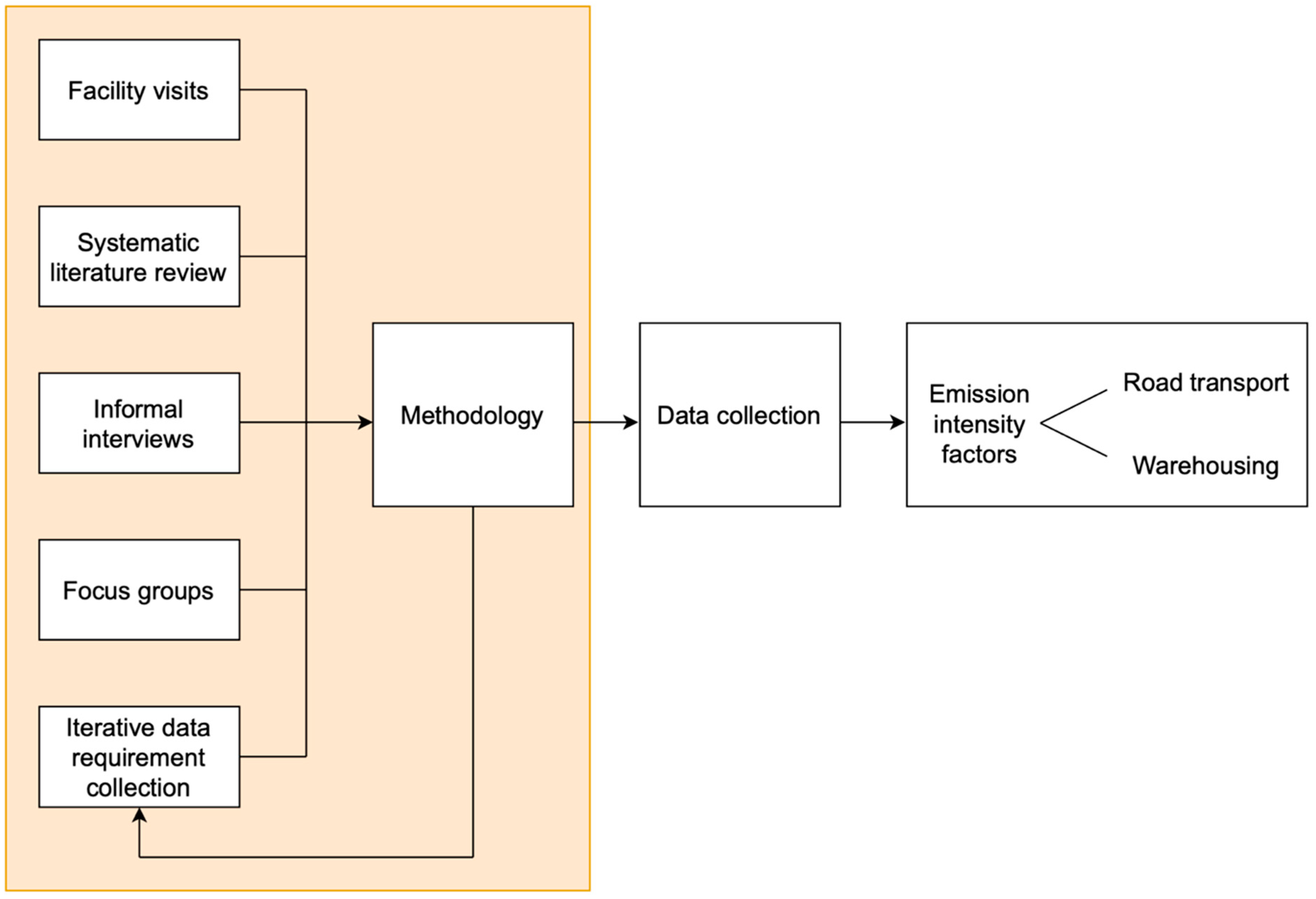
3. Methodology
4. Emission Calculation Methodology for Pharmaceutical Distribution
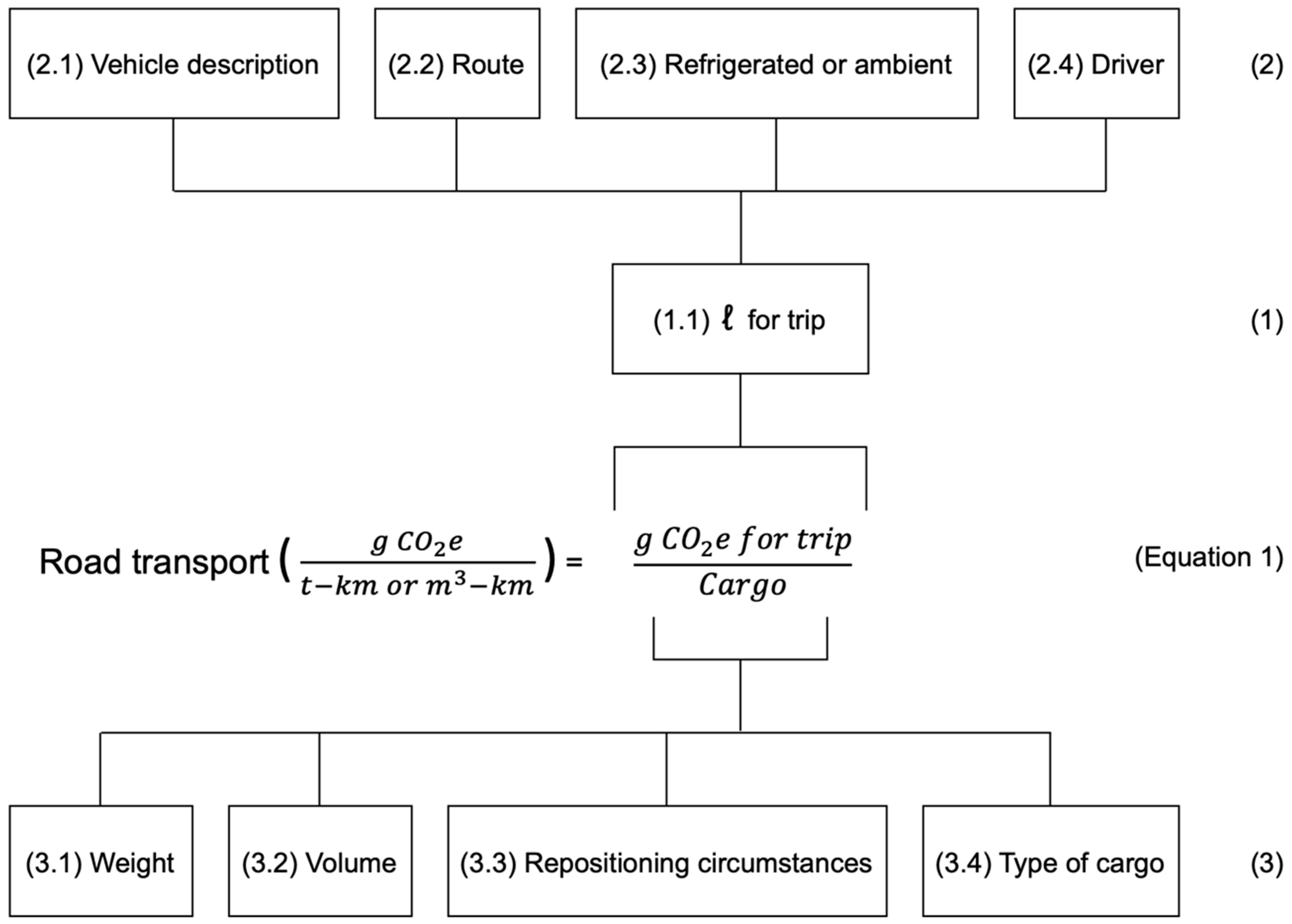
4.1. Road Transportation
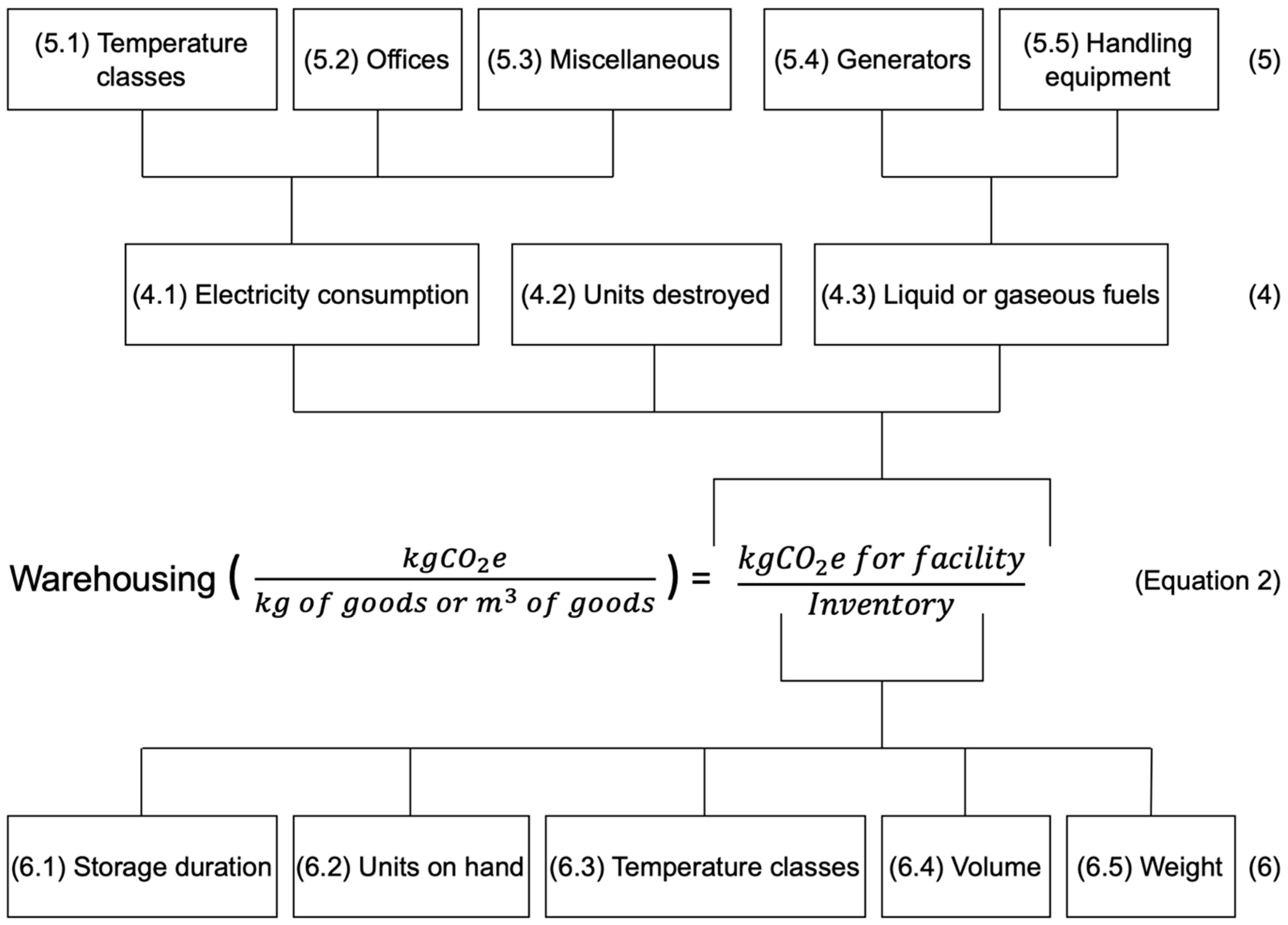
4.2. Warehousing
- Cold stores: Separated allocated areas with controlled temperatures are designed to store temperature-sensitive pharmaceutical products. Cold stores include refrigerators, freezers, and larger refrigerated rooms, for example, and should be included due to the significant contribution to the electricity consumption in the facility, which can be found in the company’s utility bill.
- Ambient cooling systems: The heating, ventilation, and air cooling (HVAC) systems used to control the temperature and humidity levels of ambient storage areas. These systems consume electricity in the process of cooling and circulating air in the warehouse, and this can be found in the energy management system and HVAC logs of the company.
- Lighting refers to types of lighting fixtures used to ensure visibility in a facility. If different parts of the facility have different types of lighting, then this variable is applicable. The contribution that lighting makes to the electricity consumption in the facility varies based on the number of fixtures, the duration of time in which the lights are operational, and their wattage. This variable can be found in utility bills as well as energy audits in the company.
- Specific machinery refers to different types of mechanical equipment that are used in the facility, such as conveyor belts, automated systems, and sorting and packing machines. This variable contributes to the electricity consumption of the facility, and its impact depends on the power rating and duration of use of the different types of machinery. This variable can be found in machine logs, OEM data sheets, energy metres on individual machines, and utility bills in the company.
5. Emission Intensity Factors for Distributing Pharmaceutical Products
5.1. Data Availability
- (a)
- The maximum empty running (%) is set at 50%. This implies that vehicles return empty for half of their trips. The reasoning behind this is that if it is greater than 50%, then logistics service providers will incur a loss and go bankrupt.
- (b)
- The minimum load factor (%) is set at 10% in terms of weight and volume. The load factor percentage represents the degree to which the vehicle’s capacity is utilised during transportation. The logic behind this assumption is that a 3PL will not load below 10% because it will cause a loss and skew the results disproportionately.
- (a)
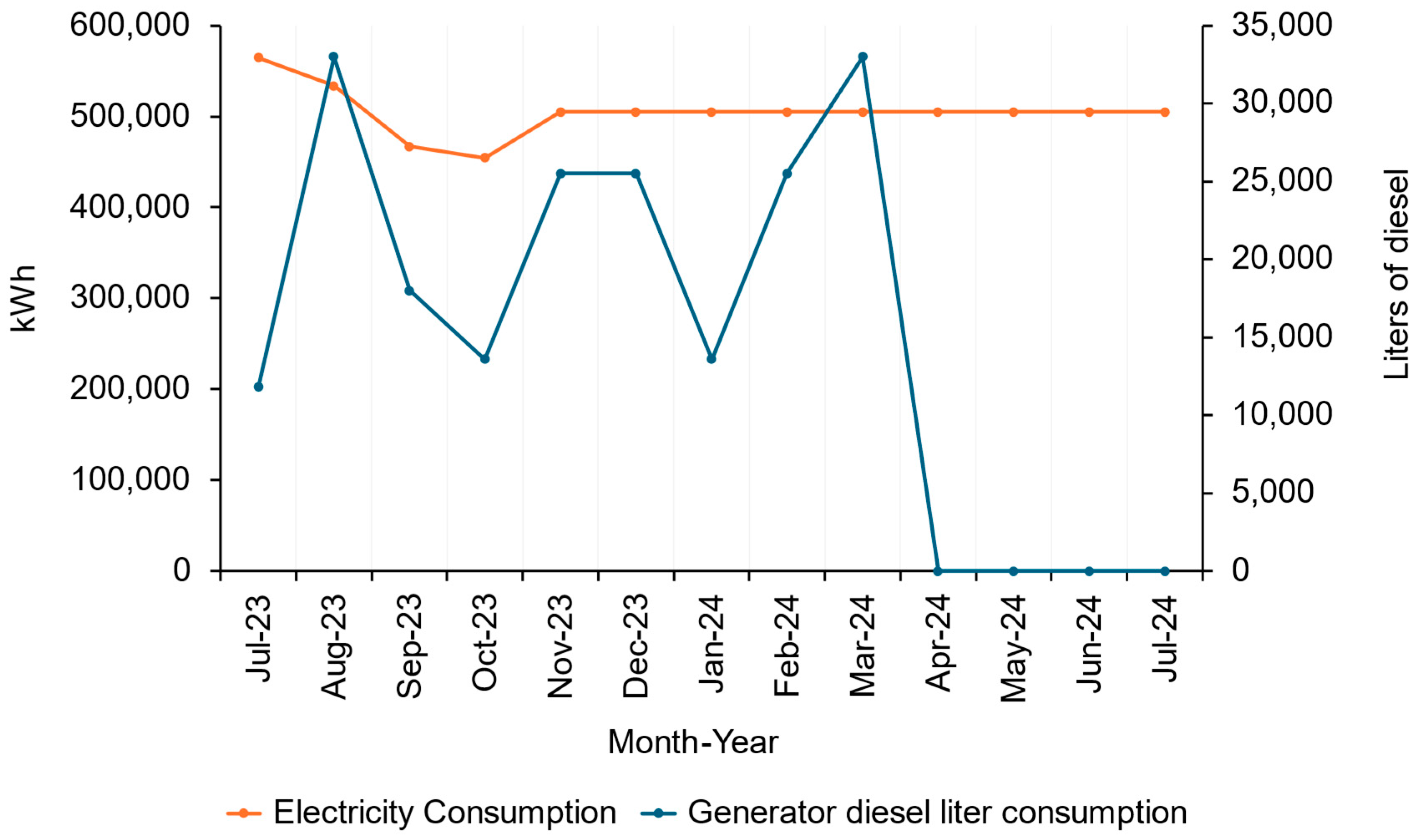
- For the months beyond October 2023 (November 2023–July 2024), electricity consumption was estimated by averaging the first four months of recorded data (July 2023–October 2023), resulting in an assumed consistent monthly consumption of 504,839 kWh. This average was applied uniformly to maintain consistency in the absence of specific monthly data.
- (b)
- To estimate diesel usage for the period November 2023–July 2024, the researchers utilised historical data on load-shedding stages. Load-shedding is a South African term used to describe deliberate and scheduled power outages implemented by Eskom to prevent the entire power grid from collapsing. Each month from July 2023 to October 2023 had a recorded load-shedding stage alongside a corresponding diesel consumption value. Where historical load-shedding stages matched those in months lacking data, the researchers assumed similar diesel consumption levels.
5.2. Results—Road Transport
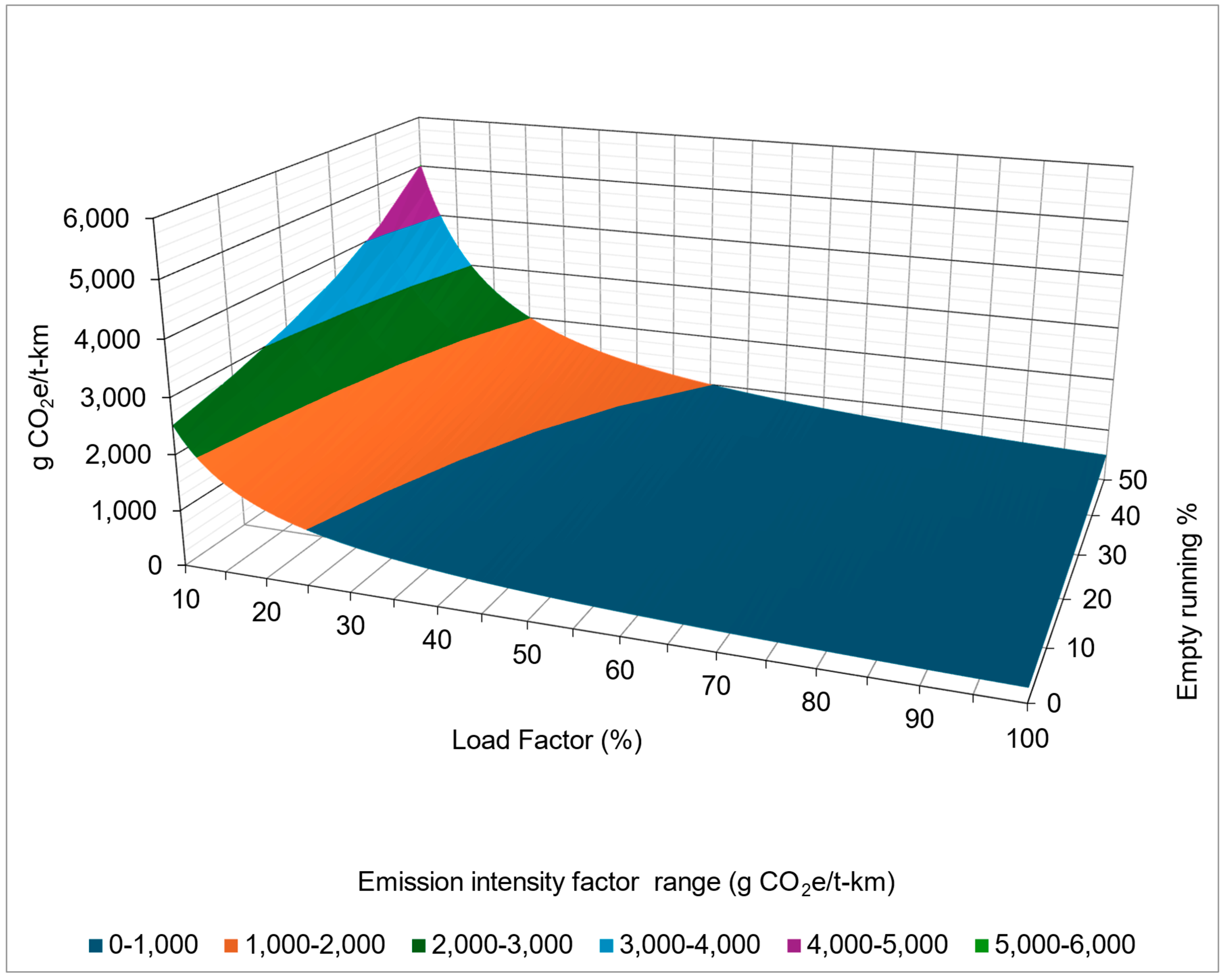
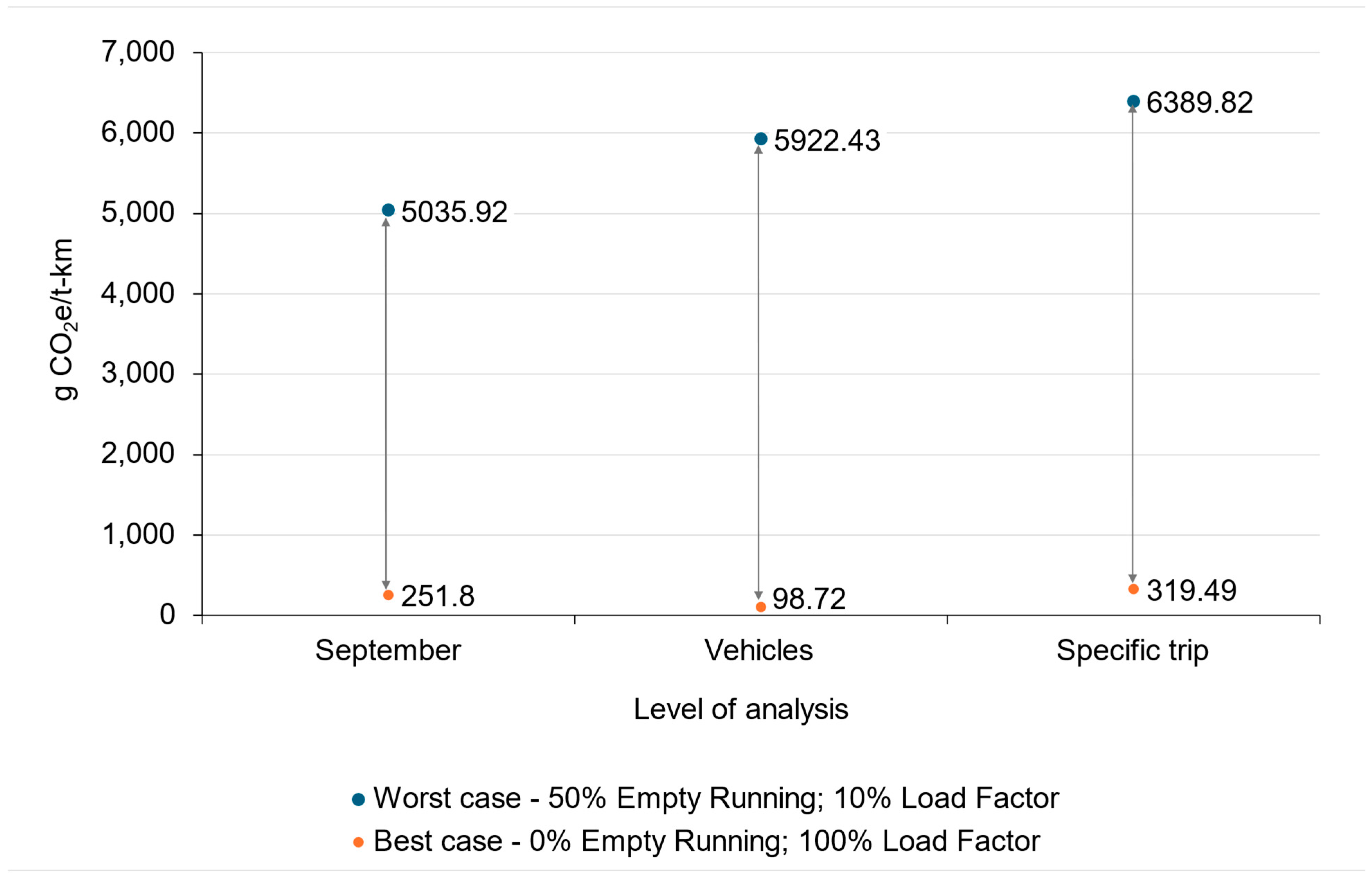
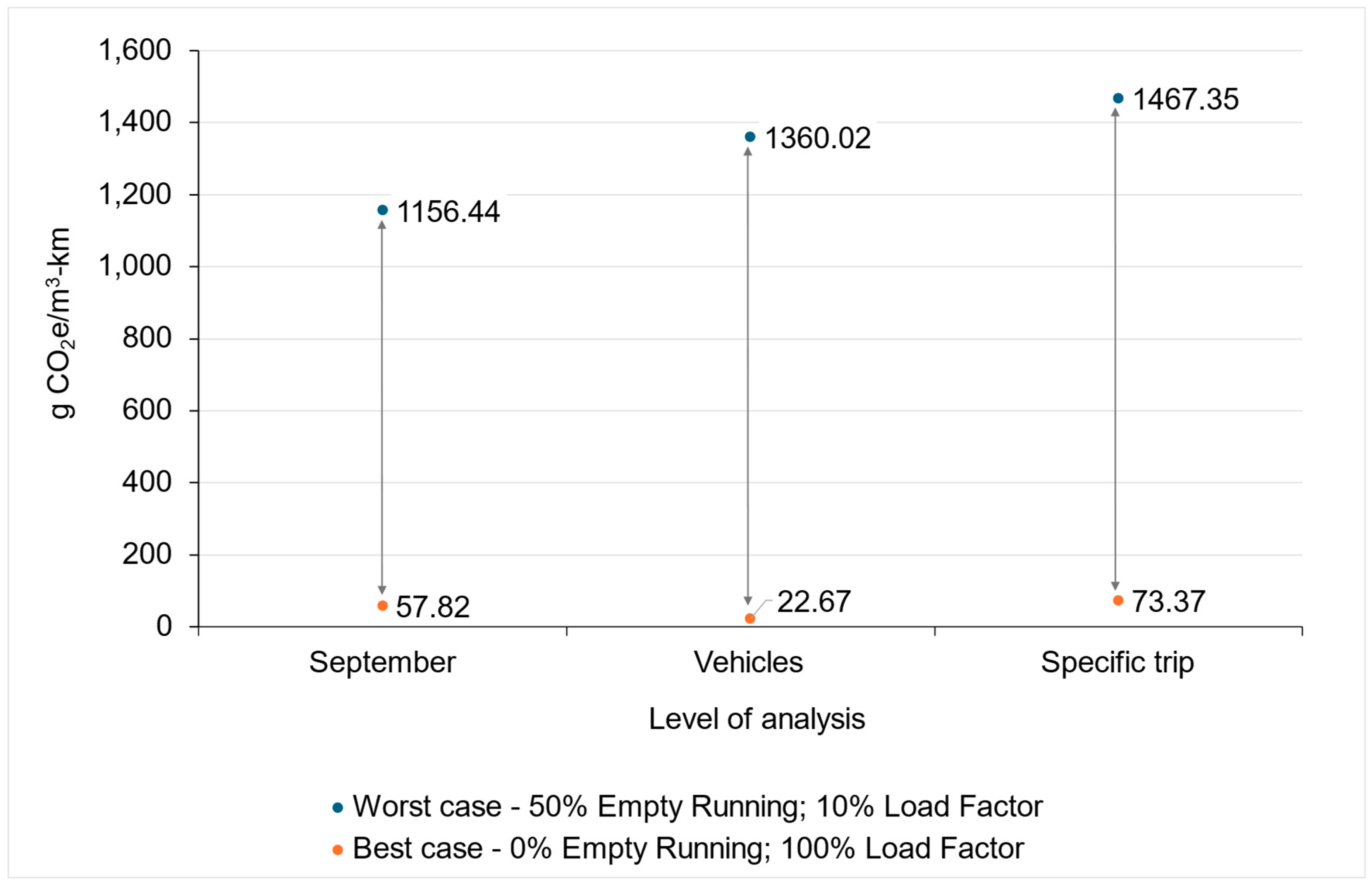
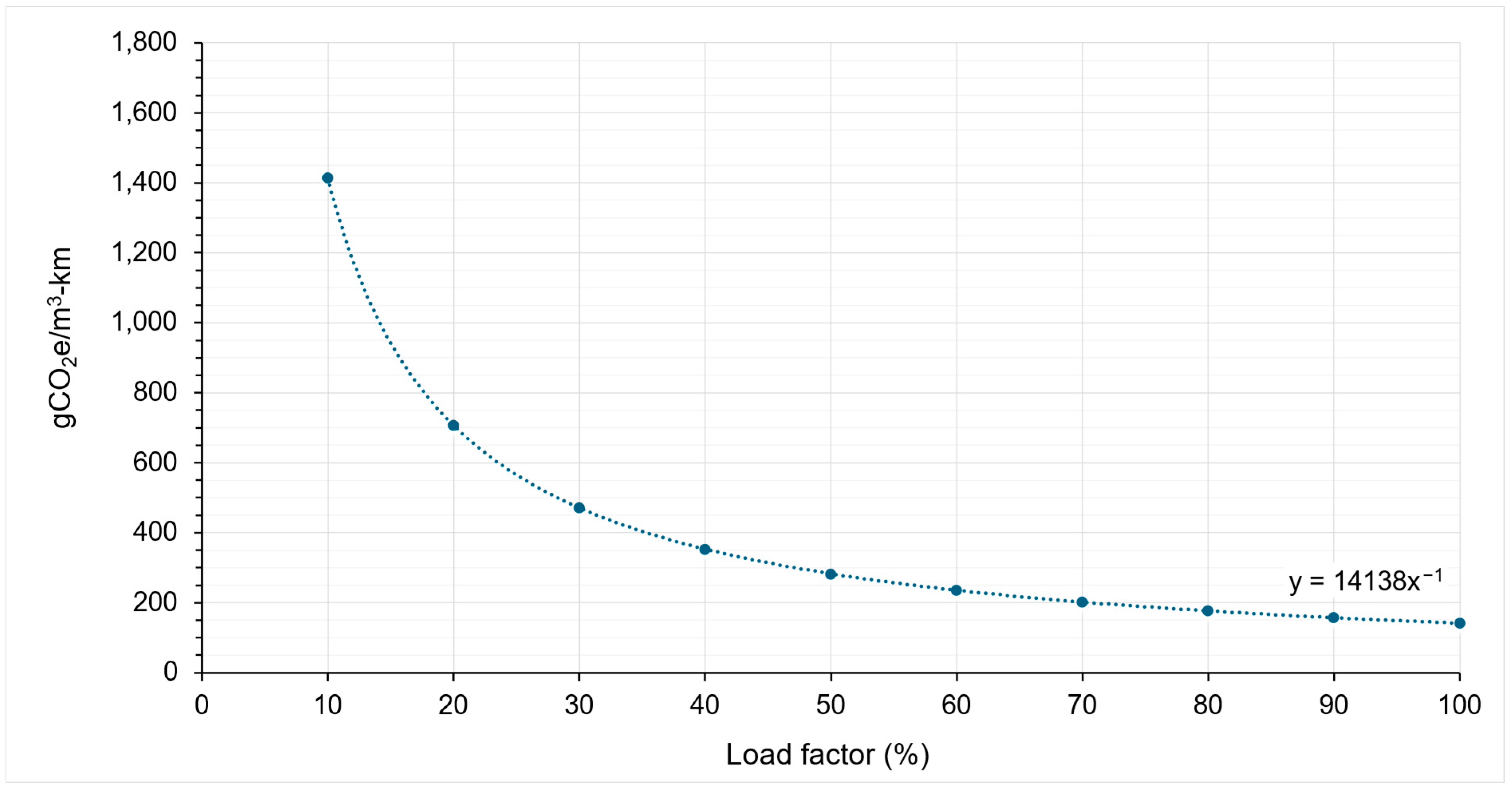
5.2.1. The Impact of Load Factor and Empty Running
- Worst case scenario (blue data points)—this scenario represents the highest emissions, with conditions of 50% empty running and a 10% load factor.
- Best case scenario (orange points)—this scenario represents the lowest emissions, with conditions of a 0% empty running and a 100% load factor.
5.2.2. Emission Intensity Factors of Road Transport
5.3. Results—Warehousing
5.3.1. Overview of the Facility
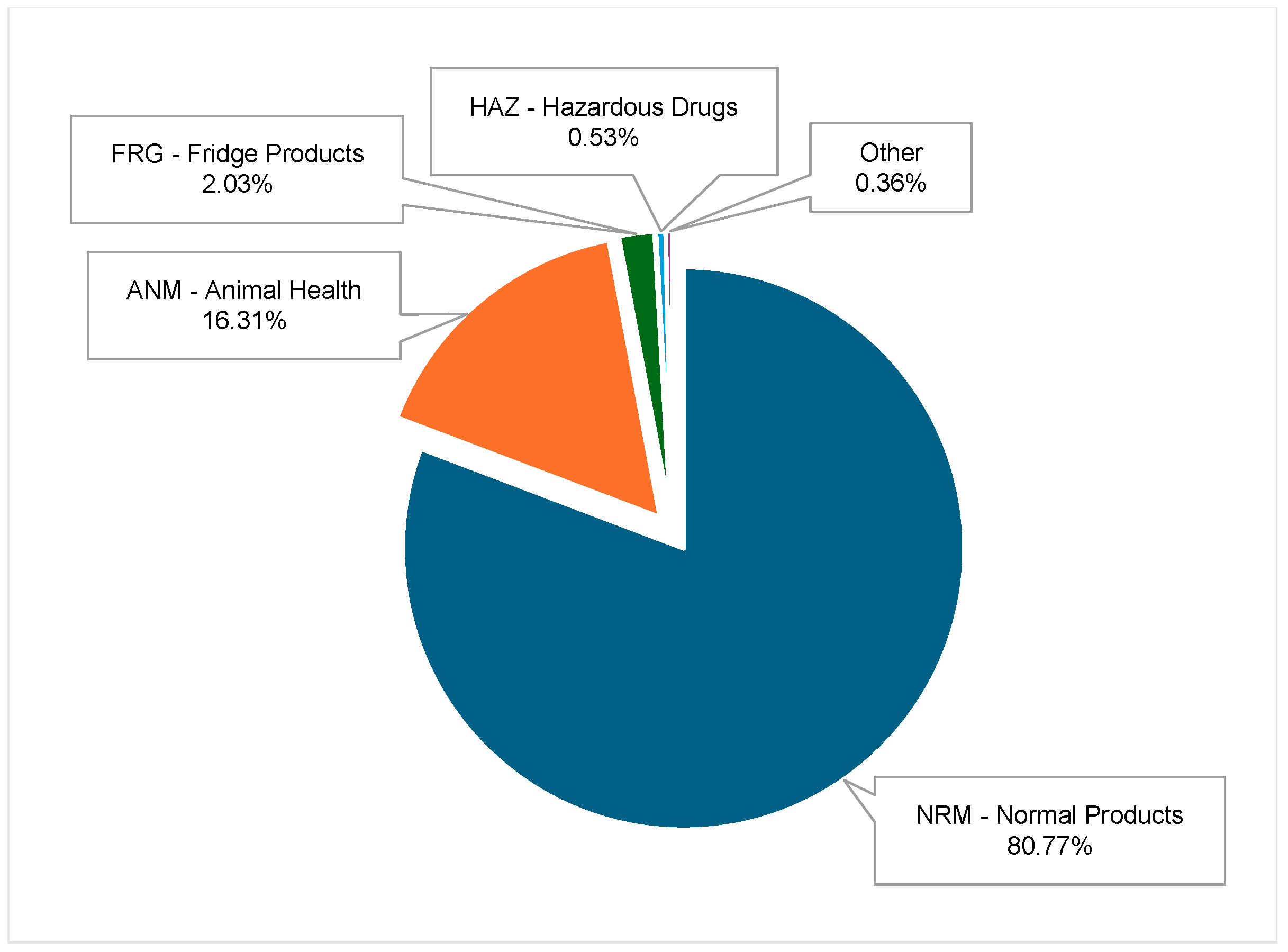
Inventory Storage Types
Energy Consumption of the Facility
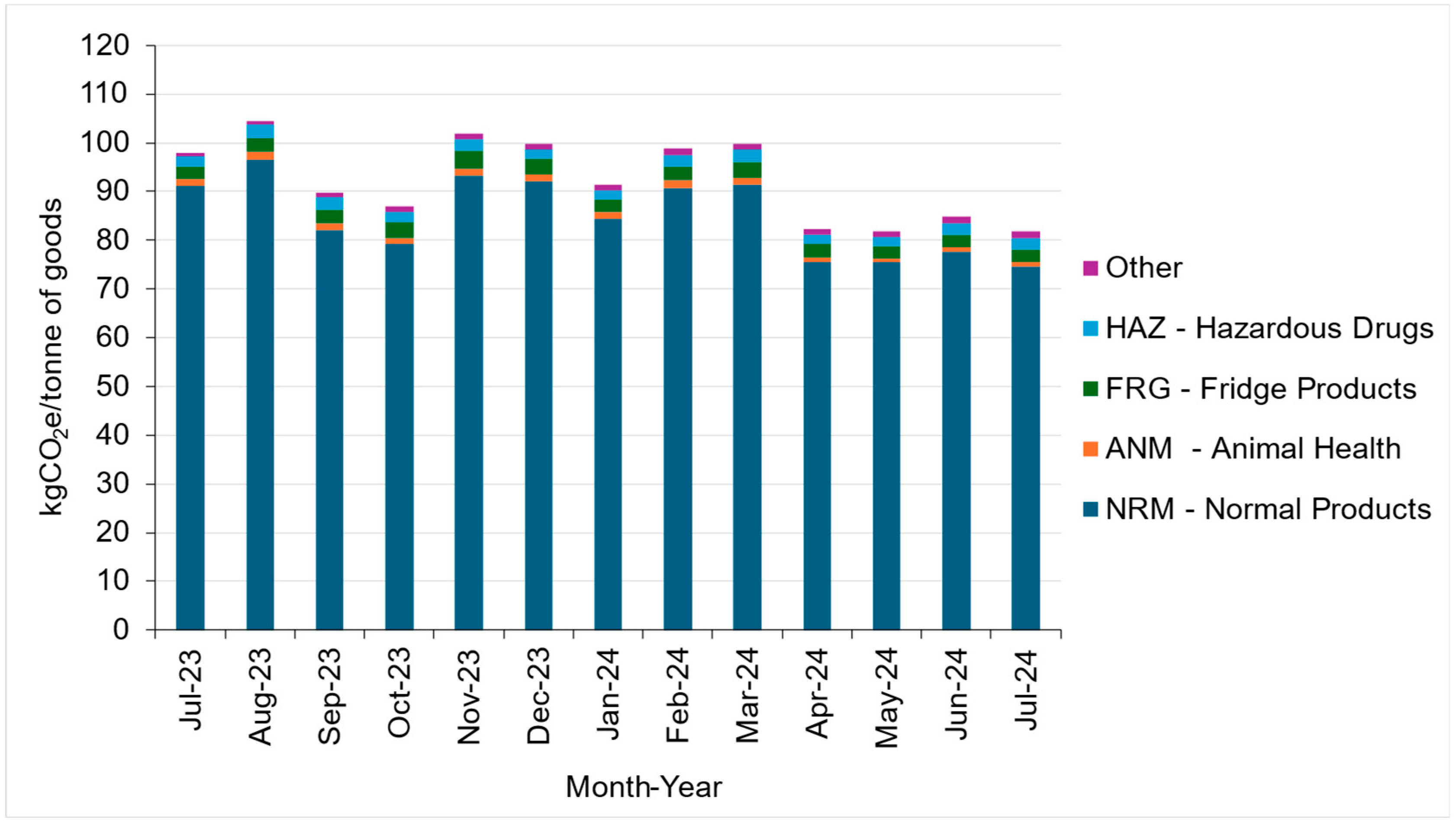
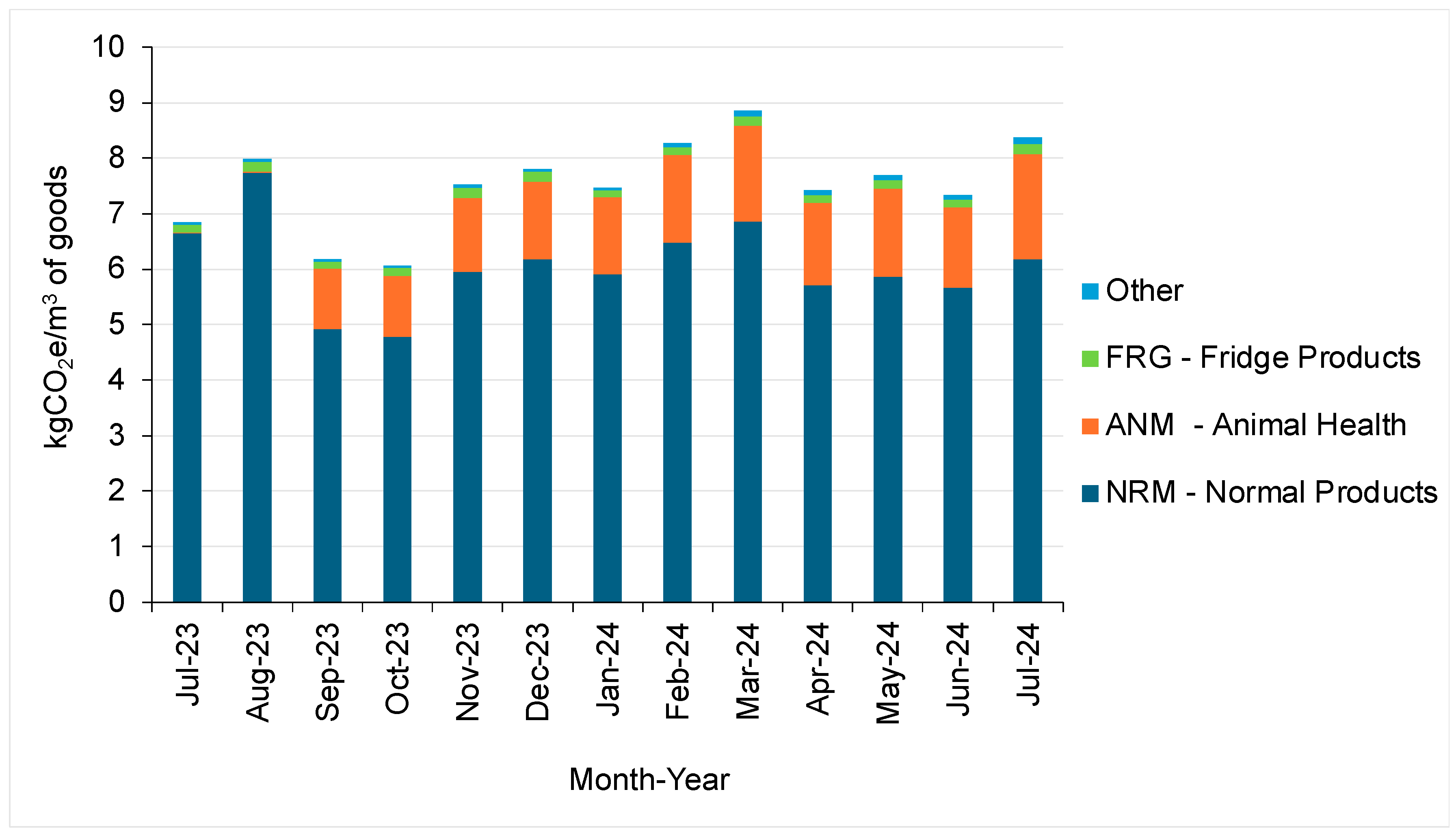
5.3.2. Emission Intensity Factor of Warehousing
6. Conclusions
Author Contributions
Funding
Institutional Review Board Statement
Informed Consent Statement
Data Availability Statement
Acknowledgments
Conflicts of Interest
Appendix A
- (a)
- = × × ×
- (b)
- = × × ×
Appendix B

| ‘Other’ for Weight Analysis | ‘Other’ for Volume Analysis |
|---|---|
| HMC—Humidity CTRL 15 to 25’C; max 60%RH | HFD—Habitat Forming drugs |
| IOD—Products containing Iodine | HFG—Hazardous and Fridge Product |
| FLM—Flammable Products | HMC—Humidity Control 15 to 25C; max 60%RH |
| FZN—Freezer Product −20 Degrees | IOD—Products containing Iodine |
| GLI—GLIADEL FRZ −20 to −25 Degrees | FRZ—Refrigerated freezer normal −15 |
| FRZ—Refrigerated freezer normal −15 | FLM—Flammable Products |
| AHH—Animal Health Hazardous | FZN—Freezer Product −20 Degrees |
| FRR—Freezer Product −10 degrees | GLI—Gliadel Freeze −20 to −25 Degrees |
| RNM—Section 21 Normal | FRR—Freezer Product −10 degrees |
| RFF—Section 21 Fridge products | FLH—Flammable and Hazardous Products |
| HFZ—Refrigerated freezer hazardous −15 | RNM—Section 21 Normal |
| RHF—Section 21 Habit-Forming Drugs | RFF—Section 21 Fridge products |
| FLH—Flammable and Hazardous Products | HFZ—Refrigerated freezer hazardous −15 |
| AHH—Animal Health Hazardous | |
| RHF—Section 21 Habit-Forming Drugs |
Appendix C
| ‘Other’ for Weight Analysis | ‘Other’ for Volume Analysis |
|---|---|
| HMC—Humidity CTRL 15 to 25’C; max 60%RH | HFD—Habitat Forming drugs |
| IOD—Products containing Iodine | HFG—Hazardous and Fridge Product |
| FLM—Flammable Products | HMC—Humidity CTRL 15 to 25’C; max 60%RH |
| FZN—Freezer Product −20 Degrees | IOD—Products containing Iodine |
| GLI—Gliadel Freeze −20 to −25 Degrees | FRZ—Refrigerated freezer normal −15 |
| FRZ—Refrigerated freezer normal −15 | FLM—Flammable Products |
| AHH—Animal Health Hazardous | FZN—Freezer Product −20 Degrees |
| FRR—Freezer Product −10 degrees | GLI—Gliadel Freeze −20 to −25 Degrees |
| RNM—Section 21 Normal | FRR—Freezer Product −10 degrees |
| RFF—Section 21 Fridge products | FLH—Flammable and Hazardous Products |
| HFZ—Refrigerated freezer hazardous −15 | RNM—Section 21 Normal |
| RHF—Section 21 Habit-Forming Drugs | RFF—Section 21 Fridge products |
| FLH—Flammable and Hazardous Products | HFZ—Refrigerated freezer hazardous −15 Degrees |
| HFD—Habitat Forming drugs | AHH—Animal Health Hazardous |
| HFG—Hazardous and Fridge Product | RHF—Section 21 Habit-Forming Drugs |
| HAZ—Hazardous Drugs |
References
- World Health Organization. Access to Medicines: Making Market Forces Serve the Poor; World Health Organization: Geneva, Switzerland, 2017. [Google Scholar]
- Duarte, I.; Mota, B.; Pinto-Varela, T.; Barbosa-Póvoa, A.P. Pharmaceutical Industry Supply Chains: How to Sustainably Improve Access to Vaccines? Chem. Eng. Res. Des. 2022, 182, 324–341. [Google Scholar] [CrossRef]
- United Nations Goal 3: Ensure Healthy Lives and Promote Well-Being for All at All Ages. Available online: https://www.un.org/sustainabledevelopment/health/ (accessed on 13 November 2024).
- Orji, I.J.; Kusi-Sarpong, S.; Huang, S.; Vazquez-Brust, D. Evaluating the Factors That Influence Blockchain Adoption in the Freight Logistics Industry. Transp. Res. Part E Logist. Transp. Rev. 2020, 141, 102025. [Google Scholar] [CrossRef]
- Du Plessis, M.J.; Van Eeden, J.; Goedhals-Gerber, L.; Else, J. Calculating Fuel Usage and Emissions for Refrigerated Road Transport Using Real-World Data. Transp. Res. Part D Transp. Environ. 2023, 117, 103623. [Google Scholar] [CrossRef]
- Hosseini Bamakan, S.M.; Ghasemzadeh Moghaddam, S.; Dehghan Manshadi, S. Blockchain-Enabled Pharmaceutical Cold Chain: Applications, Key Challenges, and Future Trends. J. Clean. Prod. 2021, 302, 127021. [Google Scholar] [CrossRef]
- Ashworth, B.; du Plessis, M.J.; Goedhals-Gerber, L.-L.; van Eeden, J. The Carbon Footprint of Pharmaceutical Distribution: A Systematic Review of Emission Methodologies. 2024; unpublished paper. [Google Scholar]
- Kramer, R.; Cordeau, J.F.; Iori, M. Rich Vehicle Routing with Auxiliary Depots and Anticipated Deliveries: An Application to Pharmaceutical Distribution. Transp. Res. Part E Logist. Transp. Rev. 2019, 129, 162–174. [Google Scholar] [CrossRef]
- Senna, P.; Reis, A.; Marujo, L.G.; Ferro de Guimarães, J.C.; Severo, E.A.; dos Santos, A.C.d.S.G. The Influence of Supply Chain Risk Management in Healthcare Supply Chains Performance. Prod. Plan. Control 2024, 35, 1368–1383. [Google Scholar] [CrossRef]
- Zighan, S.; Dwaikat, N.Y.; Alkalha, Z.; Abualqumboz, M. Knowledge Management for Supply Chain Resilience in Pharmaceutical Industry: Evidence from the Middle East Region. Int. J. Logist. Manag. 2024, 35, 1142–1167. [Google Scholar] [CrossRef]
- Zahiri, B.; Zhuang, J.; Mohammadi, M. Toward an Integrated Sustainable-Resilient Supply Chain: A Pharmaceutical Case Study. Transp. Res. Part E Logist. Transp. Rev. 2017, 103, 109–142. [Google Scholar] [CrossRef]
- Badejo, O.; Ierapetritou, M. Enhancing Pharmaceutical Supply Chain Resilience: A Multi-Objective Study with Disruption Management. Comput. Chem. Eng. 2024, 188, 108769. [Google Scholar] [CrossRef]
- Masoumi, A.H.; Yu, M.; Nagurney, A. A Supply Chain Generalized Network Oligopoly Model for Pharmaceuticals under Brand Differentiation and Perishability. Transp. Res. Part E Logist. Transp. Rev. 2012, 48, 762–780. [Google Scholar] [CrossRef]
- Mogale, D.G.; Xian, D.; Sanchez Rodrigues, V. Managing Logistics Risks in Pharmaceutical Supply Chain: A 4PL Perspective. Prod. Plan. Control 2024, 1–16. [Google Scholar] [CrossRef]
- Rajabi, R.; Shadkam, E.; Khalili, S.M. Design and Optimization of a Pharmaceutical Supply Chain Network under COVID-19 Pandemic Disruption. Sustain. Oper. Comput. 2024, 5, 102–111. [Google Scholar] [CrossRef]
- Wei, Y.M.; Chen, K.; Kang, J.N.; Chen, W.; Wang, X.Y.; Zhang, X. Policy and Management of Carbon Peaking and Carbon Neutrality: A Literature Review. Engineering 2022, 14, 52–63. [Google Scholar] [CrossRef]
- World Economic Forum Emissions. Measurement in Supply Chains: Business Realities and Challenges; World Economic Forum Emissions: Geneva, Switzerland, 2023. [Google Scholar]
- Du Plessis, M.; Van Eeden, J.; Goedhals-Gerber, L. Carbon Mapping Frameworks for the Distribution of Fresh Fruit: A Systematic Review. Glob. Food Sec. 2022, 32, 100607. [Google Scholar] [CrossRef]
- Halim, I.; Ang, P.; Adhitya, A. A Decision Support Framework and System for Design of Sustainable Pharmaceutical Supply Chain Network. Clean Technol. Environ. Policy 2019, 21, 431–446. [Google Scholar] [CrossRef]
- World Business Council for Sustainable Development, World Resource Institute (Ed.) The Greenhouse Gas Protocol: A Corporate Accounting and Reporting Standard; World Business Council for Sustainable Development: Geneva, Switzerland; World Resource Institute: Washington, DC, USA, 2004; ISBN 1-56973-568-9. [Google Scholar]
- Mejia, C.; Kajikawa, Y. Estimating Scope 3 Greenhouse Gas Emissions through the Shareholder Network of Publicly Traded Firms. Sustain. Sci. 2024, 19, 1409–1425. [Google Scholar] [CrossRef]
- Smart Freight Centre. Global Logistics Emissions Council Framework for Logistics Emissions; Smart Freight Centre: Amsterdam, The Netherlands, 2023; ISBN 978-90-833629-0-8. [Google Scholar]
- ISO BS EN ISO 14083:2023; BSI Standards Publication Greenhouse Gases—Quantification and Reporting of Greenhouse Gas Emissions Arising from Transport Chain Operations. ISO: Geneva, Switzerland, 2023.
- Eskom. Integrated Report-2022; Eskom: Johannesburg, South Africa, 2022. [Google Scholar]
- Eskom. Integrated Report-2021; Eskom: Johannesburg, South Africa, 2021. [Google Scholar]


| Activity | Basis | Vehicle Size | Emission Intensity (gCO2e/t-km) |
|---|---|---|---|
| WTW | |||
| Road transport (region dependent; Europe and South America are given as examples) |
| Van < 3.5 t | 1007 |
| Rigid truck 3.5–7.5 t GVW | 335 | |
| Rigid truck 7.5–12 t GVW | 223 | ||
| Rigid truck 12–20 t GVW | 191 |
| Hub Type Unit | Emission Intensity (kgCO2e/t) | |
|---|---|---|
| Ambient | Mixed | |
| Transshipment | 1.3 | 2.5 |
| Storage and transshipment | 5.6 | 18.4 |
| Warehouse | 45.5 | ≥50.0 |
| Logistical Activity | Data Type | Data Field or Description |
|---|---|---|
| Road Transport | Fuel data | Vehicle description: Vehicle size; Fuel type; Vehicle make; Vehicle model; Reefer unit fitted. |
| Distance travelled between refills (odometer readings) | ||
| Refill values (ℓ of fuel) | ||
| Warehousing | Facility data | Total amount of grid electricity (kWh) used |
| Total amount of diesel (ℓ) used at the facility by generators | ||
| Inventory data | Average stock on hand (units) | |
| Storage type description per SKU | ||
| Unit dimensions per SKU | ||
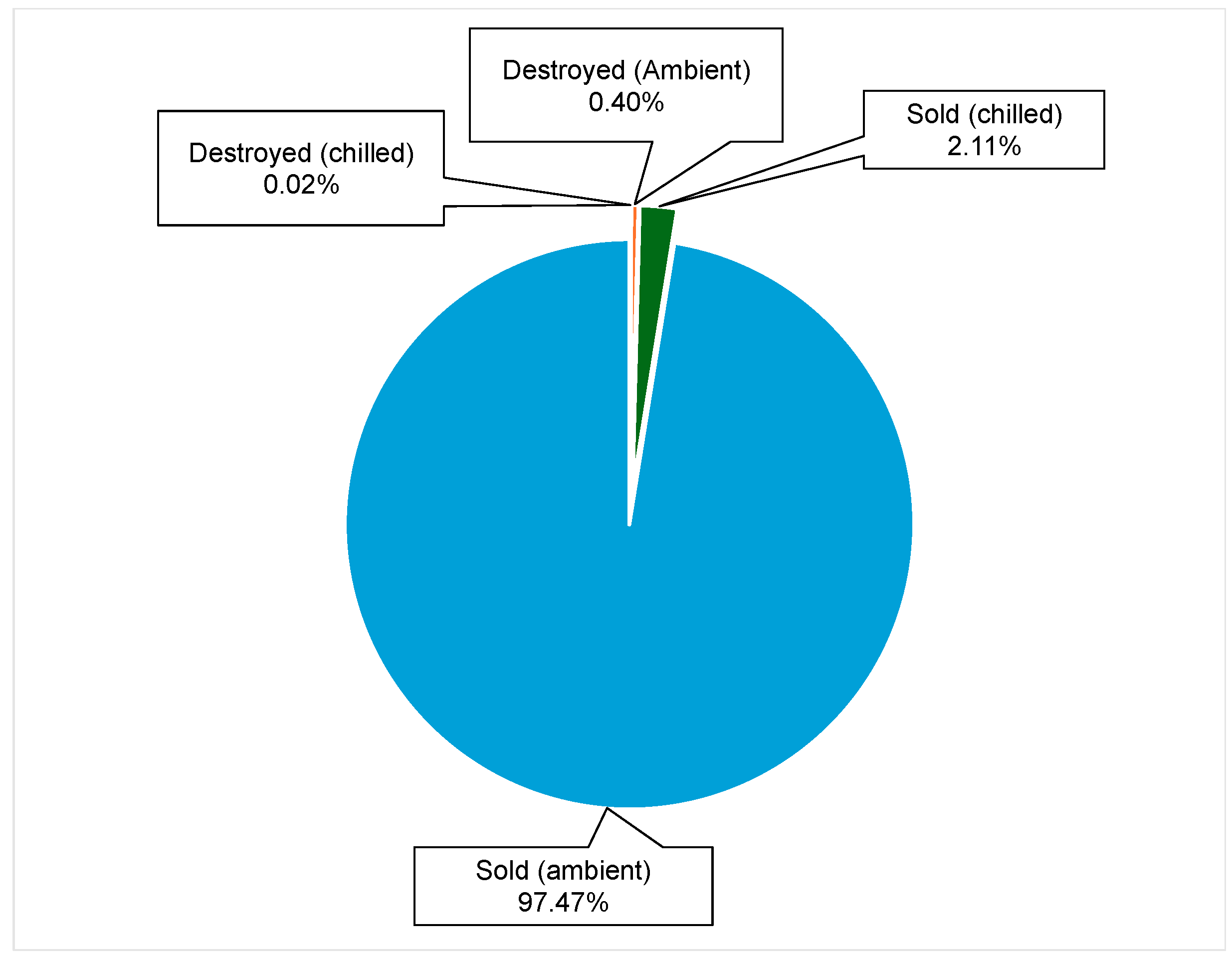
| Units destroyed per SKU |
| Weight-Based Emission Intensity Factor (EIF) (gCO2e/t-km) | Volume-Based Emission Intensity Factor (EIF) (gCO2e/m3-km) | |||
|---|---|---|---|---|
| Truck Size | Equation | Value Range | Equation | Value Range |
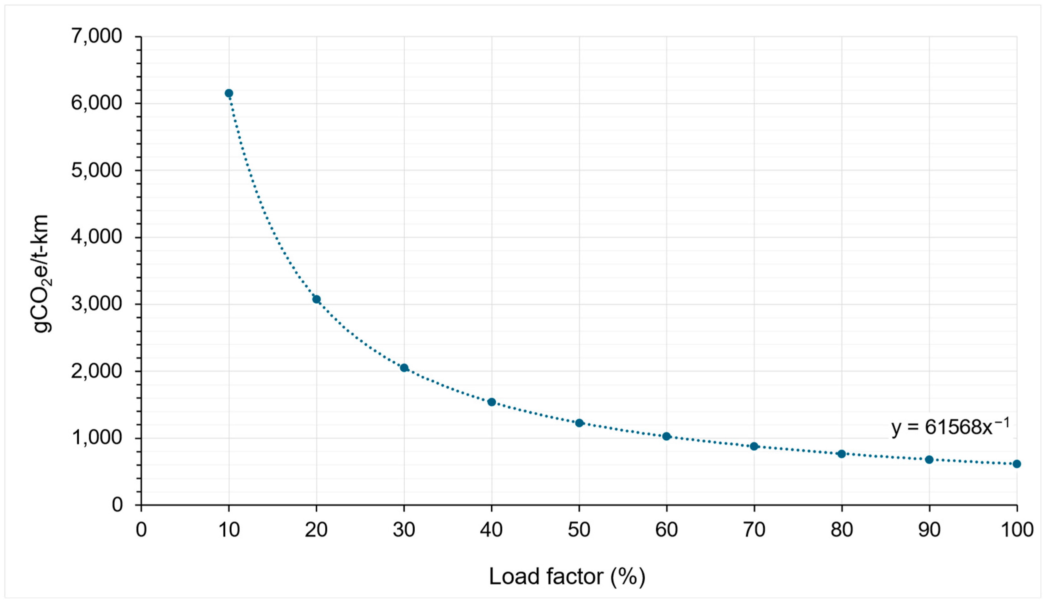
| 1-tonner | EIF1-tonner = 61,568/X | 615.68 to 6156.80 | EIF1-tonner = 14,138/X | 141.38 to 1413.84 |
| 2.5-tonner | EIF2.5-tonner = 57,037/X | 570.37 to 5703.70 | EIF2.5-tonner = 8610.7/X | 86.11 to 861.07 |
| 4-tonner | EIF4-tonner = 53,243/X | 532.43 to 5324.26 | EIF4-tonner = 6653.1/X | 66.53 to 665.31 |
| 8-tonner | EIF8-tonner = 23,957/X | 239.57 to 2395.66 | EIF8-tonner = 4574.8/X | 45.75 to 457.48 |
Disclaimer/Publisher’s Note: The statements, opinions and data contained in all publications are solely those of the individual author(s) and contributor(s) and not of MDPI and/or the editor(s). MDPI and/or the editor(s) disclaim responsibility for any injury to people or property resulting from any ideas, methods, instructions or products referred to in the content. |
© 2025 by the authors. Licensee MDPI, Basel, Switzerland. This article is an open access article distributed under the terms and conditions of the Creative Commons Attribution (CC BY) license (https://creativecommons.org/licenses/by/4.0/).
Share and Cite
Ashworth, B.; du Plessis, M.J.; Goedhals-Gerber, L.L.; Van Eeden, J. The Carbon Footprint of Pharmaceutical Logistics: Calculating Distribution Emissions. Sustainability 2025, 17, 760. https://doi.org/10.3390/su17020760
Ashworth B, du Plessis MJ, Goedhals-Gerber LL, Van Eeden J. The Carbon Footprint of Pharmaceutical Logistics: Calculating Distribution Emissions. Sustainability. 2025; 17(2):760. https://doi.org/10.3390/su17020760
Chicago/Turabian StyleAshworth, Brett, Martin Johannes du Plessis, Leila Louise Goedhals-Gerber, and Joubert Van Eeden. 2025. "The Carbon Footprint of Pharmaceutical Logistics: Calculating Distribution Emissions" Sustainability 17, no. 2: 760. https://doi.org/10.3390/su17020760
APA StyleAshworth, B., du Plessis, M. J., Goedhals-Gerber, L. L., & Van Eeden, J. (2025). The Carbon Footprint of Pharmaceutical Logistics: Calculating Distribution Emissions. Sustainability, 17(2), 760. https://doi.org/10.3390/su17020760