Optimization of Microgrid Dispatching by Integrating Photovoltaic Power Generation Forecast

Abstract

In order to address the impact of the uncertainty and intermittency of a photovoltaic power generation system on the smooth operation of the power system, a microgrid scheduling model incorporating photovoltaic power generation forecast is proposed in this paper. Firstly, the factors affecting the accuracy of photovoltaic power generation prediction are analyzed by classifying the photovoltaic power generation data using cluster analysis, analyzing its important features using Pearson correlation coefficients, and downscaling the high-dimensional data using PCA. And based on the theories of the sparrow search algorithm, convolutional neural network, and bidirectional long- and short-term memory network, a combined SSA-CNN-BiLSTM prediction model is established, and the attention mechanism is used to improve the prediction accuracy. Secondly, a multi-temporal dispatch optimization model of the microgrid power system, which aims at the economic optimization of the system operation cost and the minimization of the environmental cost, is constructed based on the prediction results. Further, differential evolution is introduced into the QPSO algorithm and the model is solved using this improved quantum particle swarm optimization algorithm. Finally, the feasibility of the photovoltaic power generation forecasting model and the microgrid power system dispatch optimization model, as well as the validity of the solution algorithms, are verified through real case simulation experiments. The results show that the model in this paper has high prediction accuracy. In terms of scheduling strategy, the generation method with the lowest cost is selected to obtain an effective way to interact with the main grid and realize the stable and economically optimized scheduling of the microgrid system.

1. Introduction

As climate change continues to intensify, the global demand for clean energy is increasing year by year. Photovoltaic (PV) power generation, an important part of clean energy, has received extensive attention worldwide. By the end of 2023, the global installed capacity of photovoltaic power generation had exceeded 1300 GW, accounting for about 18% of the global total power generation capacity. China’s installed PV capacity has ranked first in the world for many consecutive years, reaching about 500 GW, accounting for 38% of the world’s total installed PV power generation capacity. At the same time, according to the International Renewable Energy Agency (IRENA), the cost of photovoltaic power generation has fallen by about 85% over the last decade, making it one of the most economically competitive forms of energy in many countries. Photovoltaic power generation can convert solar energy into electricity without the need for fuel and does not produce harmful gases such as carbon dioxide, so photovoltaic power generation has become an effective way to solve energy shortages and improve the quality of life. Microgrids are a kind of power system that can achieve self-sufficiency. They consist of distributed power sources, loads, and energy storage systems, and can realize the efficient use and transfer of energy. Guaranteeing the stable operation and reliability of photovoltaic power generation access to a microgrid energy system is an important direction for the future development of photovoltaic power generation and microgrids [1,2]. Therefore, this paper focuses on the economic and environmental issues of different types of energy scheduling in microgrids, integrates the results of PV power generation prediction, and performs scheduling optimization of microgrid power system.

As photovoltaic power generation brings significant economic and environmental benefits, it has received more and more attention, and research on photovoltaic power generation prediction tends toward machine learning, deep learning, and neural networks [3].

The advantage of the machine learning approach is that it is able to model a wide range of dynamic processes. In the study of Leva S. (2017) [4], Artificial Neural Network (ANN) was used for photovoltaic power generation forecasting. The study pointed out that the accuracy of the historical dataset has a significant impact on the accuracy of the model. Popular AI models developed by some researchers such as Tan (2020) [5] for RPGP include Support Vector Machines (SVM). Compared to statistical methods, AI models have higher prediction accuracy for EPGP. However, these models are based on shallow architectures, require manual feature engineering, have limited generalization capabilities, and lead to unstable networks and non-convergence of parameters due to insufficient EPGP data. Deep learning methods have been widely used in the process of digitization and intelligent transformation of various industries, and can also be used for photovoltaic power generation forecasting. Aslam (2021) [6] and others outlined deep learning-based methods for predicting solar panel and wind turbine power generation. Due to their self-learning capability, various ANN-based building energy consumption prediction models have been developed. Kim (2020) [7] found neural network models to be more valuable and stable than linear regression methods in predicting electricity loads. Optimization methods have also been introduced in some studies to improve computational efficiency. For example, Kalliola (2021) [8] et al. developed neural network models to predict real estate prices, providing solutions for fine-tuning hyperparameters using stochastic search. Zhou (2021) [9] developed an adaptive hyperparameter tuning model for predicting fuel consumption of ships. Bayesian optimization was used to select the optimal neural network structure, support vector machine, minimum absolute contraction, random forest, and selection operator. However, in practice, photovoltaic power generation is affected by many environmental stochastic factors, resulting in the collected data possibly containing noise, missing information, or errors, which leads to an increase in the difficulty of model training and affects the prediction results. Different deep learning models have different advantages, so the prediction results of an algorithm are further optimized and improved by establishing a combined prediction model. Netsanet S (2022) [10] proposed a hybrid method, VMD-ACO-2N, wherein the raw data are decomposed using variational modal decomposition (VMD), and the optimization setup is performed through a method involving orthogonal indices (OIs) and correlation measures. The method was shown to outperform other algorithms when feature contributions all played a role. Liang L (2023) [11] proposed a short- and medium-term PV power prediction model based on FC, DT, LSSVR and IWBOA, with predictions able to be made for time scales of one day ahead and one month ahead. The computational speed and prediction accuracy of the LSSVR model were improved by optimizing each independent sub-model through IWBOA. The model is important for the availability and grid integration benefits of PV power generation.

In summary, traditional machine learning models and statistical approach models still have limitations in photovoltaic power generation forecasting. There are still problems such as difficulty in fully capturing data features and low accuracy. However, deep learning is very effective in feature extraction of data, especially in photovoltaic power generation forecasting, where deep learning has achieved better results. In the photovoltaic power generation forecast of distributed multiple stations, a single model has disadvantages, such as low generalization ability and poor learning ability. In order to improve the efficiency as well as accuracy of photovoltaic power generation forecasts, this paper constructs a hybrid neural network photovoltaic power generation forecast model and designs an improved CNN-BiLSTM model.

The research on microgrid power scheduling is more in the direction of microgrid systems, distributed energy scheduling, etc. Dhiman G (2020) [12] proposed a novel hybrid multi-objective algorithm, MOSHEPO, for solving convex and non-convex economic scheduling and microgrid power scheduling problems. MOSHEPO takes into account many of the nonlinear characteristics of generators, such as transmission losses, multiple fuels, valve point loads, and prohibited operation areas, as well as their operating limitations, to inform the model and improve its suitability for real-world operation. Prasad T N (2022) [13] proposed a hybrid AC/DC microgrid power management strategy using Droop control. The scheme uses ANFIS and PID controllers to control microgrids with energy sources such as PV, wind, and batteries, and achieves operational cost reduction through an elephant swarm optimization algorithm, which in turn calculates Droop coefficients to implement an adaptive Droop control strategy. Luo S (2023) [14] proposed a multi-objective microgrid power scheduling method for optimal output power of distributed generators. A two-step solution method based on chaotic sinusoidal mapping multi-objective optimization bat algorithm and fuzzy theoretical set is used to solve the problem. In summary, renewable energy, represented by wind and solar energy, has been rapidly developed in the process of the rapid improvement of energy structure. In this paper, we take advantage of the combination of distributed energy sources in microgrids in order to improve the ability of microgrids to accept and dispatch renewable energy sources, and to achieve the complementary integration of multiple types of power sources in order to maximize the overall benefits.

In this paper, for the uncertainty and intermittency of the photovoltaic (PV) power generation system, a microgrid scheduling model including PV power generation prediction is proposed, classifying PV power generation data through cluster analysis, combining Pearson’s correlation coefficient and PCA downscaling to analyze the key features, constructing a combined prediction model based on SSA-CNN-BiLSTM, and introducing an attention mechanism to improve the prediction accuracy; subsequently, a multi-temporal dispatch optimization model is established based on the prediction results, and a differential evolution improvement quantum particle swarm optimization algorithm is introduced to solve the problem with the objective of optimizing the economic and environmental costs, and the effectiveness and feasibility of the model and the algorithm are verified through the simulation of real cases.

The following are the research features and innovations of this paper:

(1)

This paper presents an in-depth study on the application of new energy photovoltaic power generation, and proposes an effective forecasting and scheduling method, which better solves the imbalance in the distribution of microgrid power resources due to the volatility of renewable energy production.

(2)

In terms of photovoltaic power generation forecast, this paper proposes a neural network model based on CNN-BiLSTM, which can consider multiple influencing factors in the process of photovoltaic power generation at the same time to make the forecasting results more accurate.

(3)

This paper introduces the group intelligence algorithm in the prediction model to optimize the original structure. Sparrow search algorithm is used to optimize the weights as well as the thresholds of the CNN-BiLSTM neural network to improve the robustness of the model and to increase the attentional mechanism to improve the predictive accuracy of the model while reducing the computational cost more, and to improve the generalization ability of the model.

(4)

A microgrid distributed power scheduling model is established by this paper, which focuses on how to reasonably allocate the weights of economic objectives as well as environmental objectives in the multi-objective scheduling problem, and introduces the quantum particle swarm algorithm based on differential evolutionary algorithm to solve the problem, and constructs an optimization model aimed at minimization of the system operation cost.

2. Photovoltaic Power Generation Prediction Model Based on Cluster Analysis and SSA-CNN-BiLSTM-ATT

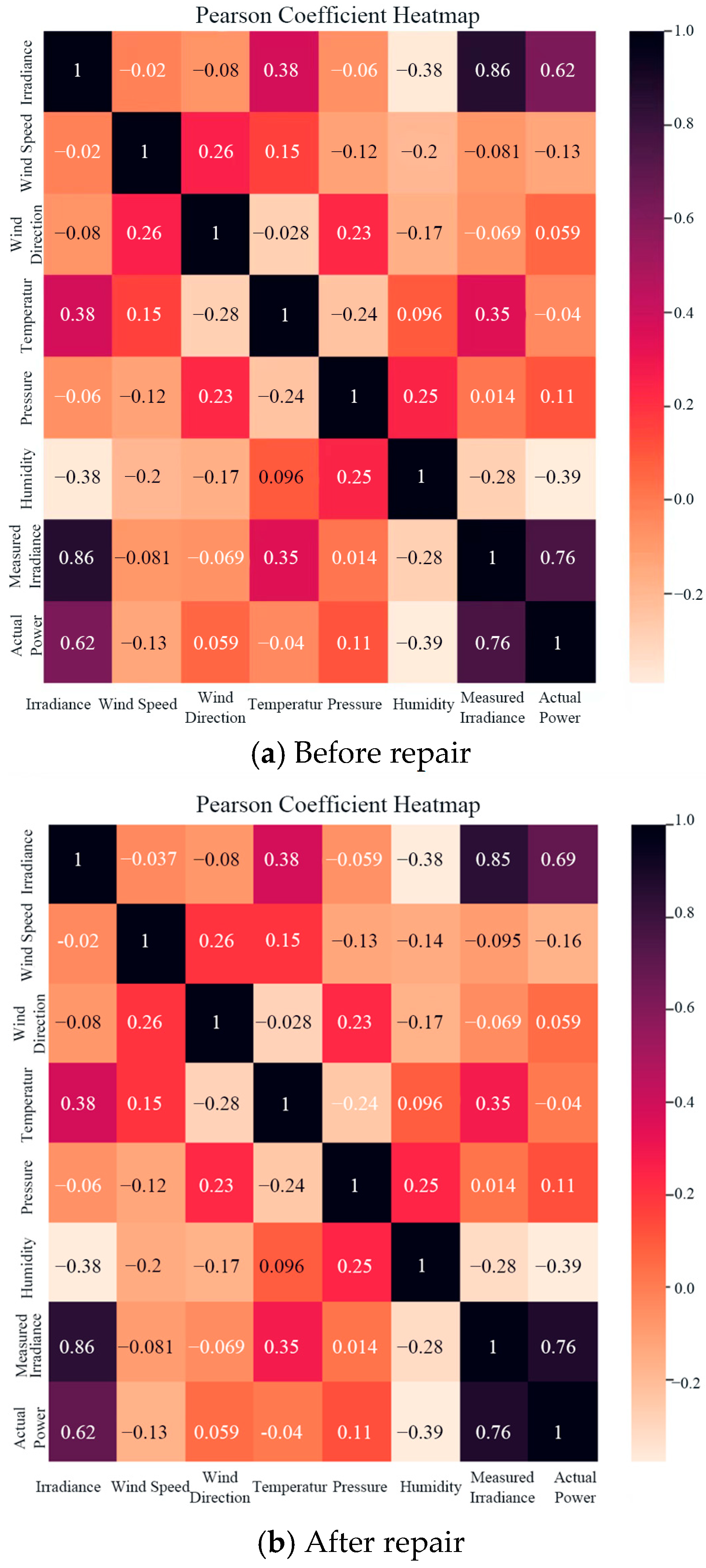
2.1. Correlation Analysis of Influencing Factors

Photovoltaic power generation harnesses the energy of solar cells by converting light into electricity. When photons enter a solar cell, their energy is absorbed by the semiconductor material, exciting electrons to a higher energy state and creating electron–hole pairs. Driven by the internal electric field of the cell, electrons flow from the N-region to the P-region, while holes move in the opposite direction, generating an electric current and effectively transforming light energy into electrical energy. The main influencing factors of photovoltaic power generation are classified into the time dimension as well as non-time dimension, which mainly include climatic condition, module type, location of the power plant and human factors. For meteorological factors, humidity, temperature, wind direction, wind speed, and air pressure are selected as meteorological parameters in this paper. For geographic factors, the regional environment of the PV system, geographic coordinates, and altitude are selected.

In order to quantify the influence of each feature on the PV power, the Pearson correlation coefficient metric is introduced in this paper. The Pearson correlation coefficient metric can quantify the influence of irradiance, temperature, wind speed, and humidity, as shown in

Table 1. Value range of Pearson correlation coefficient.

Relevant Relation		Degree of Relevance
$\left|R_{mn}\right|=1$	Perfect linear correlation	$\left|R_{mn}\right|\le 0.2$	extremely weak correlation
$R_{mn}=0$	no linear correlation	$0.2<\left|R_{mn}\right|\le 0.4$	weak correlation
$0<R_{mn}<1$	positive correlation	$0.4<\left|R_{mn}\right|\le 0.6$	moderately relevant
$-1<R_{mn}<0$	negative correlation	$0.6<\left|R_{mn}\right|\le 0.8$	strong correlation
		$0.8<\left|R_{mn}\right|\le 1.0$	Highly relevant

.

The Pearson correlation coefficient is calculated as:

$$R(m,n)={\displaystyle \frac{{\displaystyle {\sum }_{j=1}^l(m_j-\overline{m})(n_j-\overline{n})}}{\sqrt{{\displaystyle {\sum }_{j=1}^l{(m_j-\overline{m})}^2}}\sqrt{{\displaystyle {\sum }_{j=1}^l{(n_j-\overline{n})}^2}}}}$$

(1)

in which m is the power generated by the photovoltaic power generation mechanism at one time, $m=\left[m_1,m_2,\dots ,m_l\right]$; n is the historical meteorological impact factor of the PV generation produced by the input generating organization, $n=\left[n_1,n_2,\dots ,n_l\right]$; l denotes the number of samples; m_j is the power of the PV plant on day j and $\overline{m}$ is the jth average of the historical power of the photovoltaic power generation m; n_j is the meteorological impact factor for day j of the PV plant; $\mathrm{n} ¯$ is the jth average of the historical meteorological impact factor n of the photovoltaic power generation. The first inertia between the two variables is greater when $R\left(m, n\right)$ is closer to −1 or 1.

In this paper, the actual power of a photovoltaic power plant with wind direction and wind speed data on 30 March 2018 is chosen. Figure 1 is plotted using the pandas library in Python. Figure 1a represents the heatmap of Pearson’s correlation coefficients containing the features before fixing, while Figure 1b shows the heatmap of Pearson’s coefficients after applying the K-Nearest Neighbor (KNN) algorithm to fix the anomalous data.

According to Figure 1, it can be concluded that among the multiple meteorological factors affecting the output of photovoltaic power generation, the Pearson correlation coefficient between the actual irradiance before restoration and the actual power generation of photovoltaic power generation is 0.76. After removing the outliers, the correlation coefficient improves to 0.88, indicating that the linear correlation between the two is further enhanced. In practical PV power prediction tasks, the model is usually trained using measured irradiance and predicted using forecasted irradiance. In Figure 1b, after fixing the data used, the coefficient between the predicted irradiance and the PV generation of the generating organization increased from 0.62 to 0.69, an improvement of 0.07.

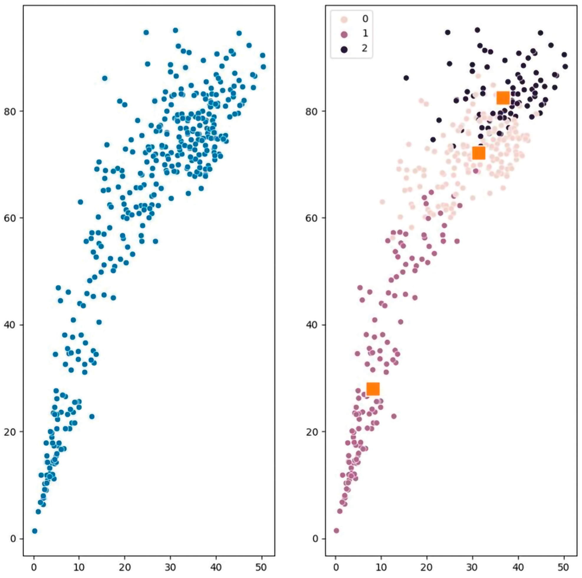
2.2. Data Preprocessing Based on Fuzzy C-Means Algorithm

Photovoltaic power generation is affected by the day–night turnover, which exhibits an obvious cyclic pattern. In order to improve the prediction accuracy, a fuzzy C-means algorithm is introduced to preprocess the data. By using fuzzy C-mean clustering, the weather is classified into sunny, rainy, and complex types of weather, and then the prediction models are established for these three types of weather, respectively.

2.2.1. Cluster Analysis of Photovoltaic Data

Three historical similar day datasets are obtained using the fuzzy C-means algorithm of clustering and the prediction models are trained using the historical datasets under different weather types, respectively. The clustering results of this paper are shown in Figure 2, where the left graph represents before clustering, the right graph represents after clustering, the Y-axis represents the PV power, the X-axis represents the data series, the yellow squares indicate the centroids of the data clustering results, and 0, 1, 2 in the graph correspond to rainy, complex weather and sunny days, respectively.

The principle of the fuzzy clustering algorithm is described as follows. Assuming that there is a dataset $X=\left\{x_1,x_2,x_3,\dots ,x_n\right\}$, the data in dataset X are first classified into C fuzzy sub-datasets: $\left\{A_i\left|i=1,2,\dots ,C\right.\right\},0\le C\le n$, where C_i is the clustering center of class i and the affiliation degree of class i samples is U_ij. The target dependent variable in the fuzzy C-means algorithm is shown in Equation (2):

$$J(U,V)={\displaystyle \sum _{i=1}^C{\displaystyle \sum _{j=1}^n{u}_{ij}^m}}{‖x_j-c_i‖}^2$$

(2)

where U is the fuzzy C classification of the dataset X, and $V=\left\{v_1,v_2,\dots v_n\right\}$ is the clustering center. m is the weighting factor for the degree of affiliation, and fuzzy clustering is hard C-means clustering when m = 1. m is usually taken as 1.5–2.5, and in this paper, m = 2.

The constraints are:

$${\displaystyle \sum _{i=1}^c{u}_{ij}=1, j=1,2,}\dots ,n$$

(3)

$${\displaystyle \sum _{i=1}^c{u}_{ji}=1, }0<{\displaystyle \sum _{j=1}^n{u}_{ji}}<n$$

(4)

The Euclidean distance between the data object and the obtained cluster center v_i is:

$$d_{ij}=‖x_j-v_i‖$$

(5)

J(U, V) is a function that is used in the algorithm to calculate the sum of squares of the errors between the original data objects and the known cluster centers, and its value reflects the closeness and correlation between the data objects and the cluster centers. When the value of J(U, V) is smaller, the degree of closeness of the clusters is higher. Set C = 1; the smaller the value of C, the higher the degree of closeness of the clusters.

The following is the main computational procedure of the fuzzy C-means algorithm:

(1)

Initialization of the clustering center, $V=\left\{v_1,v_2,\dots v_n\right\}$.

(2)

Calculate the different affiliation matrices:

$$u_{ij}={\displaystyle \frac{1}{{\displaystyle \sum _{k=1}^c{\left(\frac{‖x_i-c_j‖}{‖x_i-c_k‖}\right)}^{\frac{2}{m}}}}}$$

(6)

(3)

Update the clustering center:

$$c_j={\displaystyle \frac{{\displaystyle {\sum }_{i=1}^N{u}_{ij}^m{x}_i}}{{\displaystyle {\sum }_{i=1}^N{U}_{ij}^m}}}$$

(7)

(4)

Repeat (2) and (3) until Equation (2) converges and reaches the maximum number of iterations.

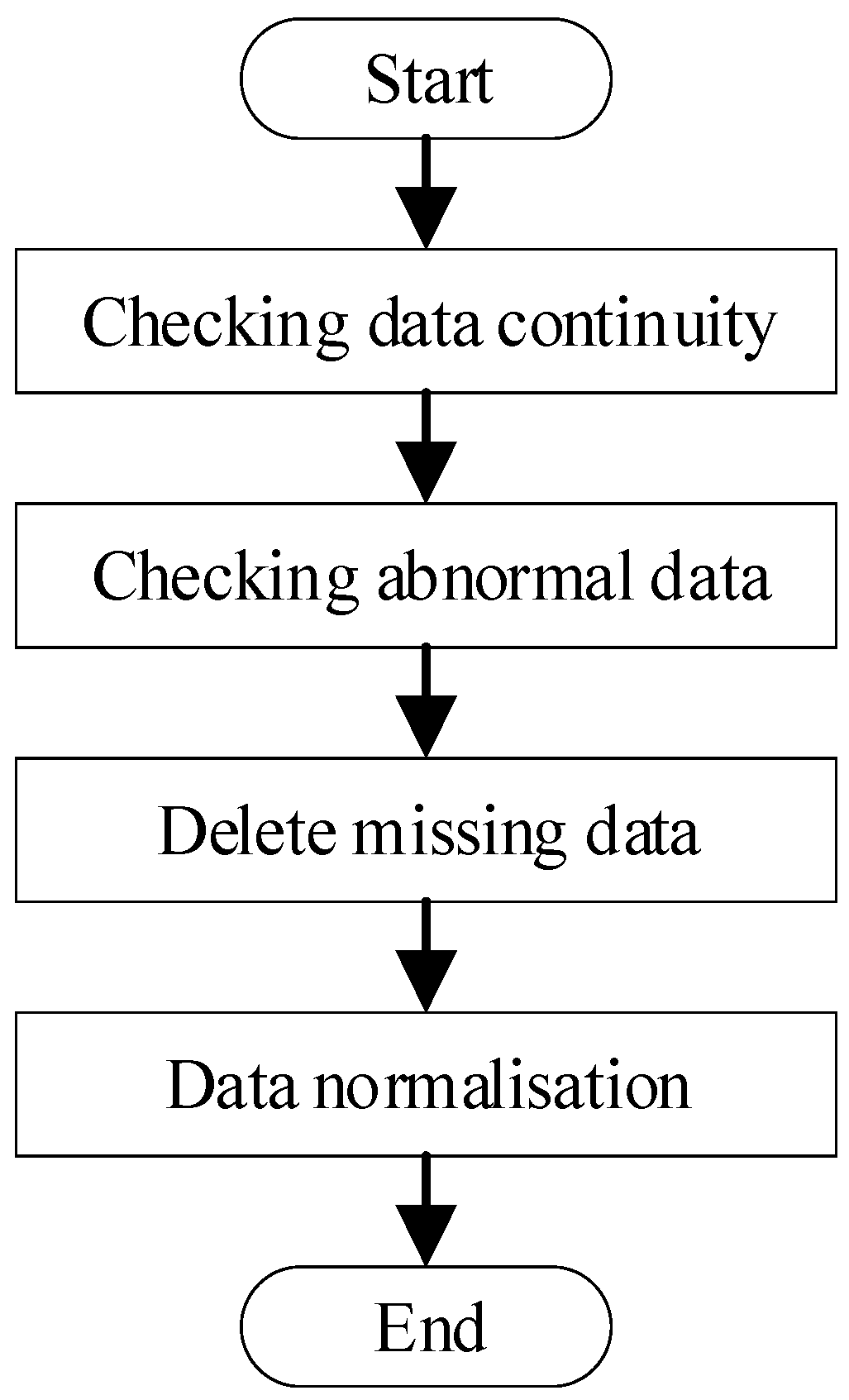
2.2.2. Photovoltaic Data Preprocessing

In this paper, the PV power plant data used were obtained from a portion of a PV power plant with a maximum installed capacity of 50.00 MW in a region of China. This paper uses the data provided by this photovoltaic power generation station to carry out a prediction study on photovoltaic power generation. The data preprocessing process is shown in Figure 3 below.

The specific flow of the preprocessing step for the data used in this paper is shown below:

(1)

Check the continuity of the data and mark missing or duplicate data points. The timestamp format can be used to calculate the time difference between two consecutive points.

(2)

Remove anomalous data based on the maximum power value.

(3)

Remove consecutive missing power data.

(4)

Normalize the data to remove unit differences between different factors.

Numerical normalization refers to the uniform mapping of data of different magnitudes to the same order of magnitude to eliminate the effect of their respective magnitudes. The minimum–maximum method is calculated as shown in Equation (8):

$$x^{\ast }={\displaystyle \frac{x-x_{\min }}{x_{\max }-x_{\min }}}$$

(8)

The normalized value is $x^{\ast }$, the maximum value is X_max and the minimum value is X_min. The mean value method is calculated as shown in Equation (9):

$$x^{\ast }={\displaystyle \frac{x-x_{mean}}{x_{\mathrm{var}}}}$$

(9)

$x^{\ast }$ denotes the normalized value, $x_{mean}$ denotes the mean value of x, and $x_{\mathrm{var}}$ denotes the variance of x.

2.2.3. Data Dimensionality Reduction Based on Principal Component Analysis

After going through data preprocessing, there is still a lot of unnecessary information in the data. Therefore, in this paper, the data are downscaled through feature selection as well as feature transformation. The main principle of the Principal Component Analysis (PCA) method is to turn high-dimensional variables into low-dimensional variables, while ensuring that the original variables retain a good representation. This allows for the data transformation of the overall sample of the dimensionality reduction process [15].

(1)

The core idea of PCA is a matrix compression algorithm that converts the original matrix of $n\times m$ into a lower dimensional matrix of $n\times k$.

(2)

Inputs $X_1,X_2,\cdots ,X_m$ in the model of PCA are the original variables, and the target variables $Y_1,Y_2,\cdots ,Y_k$ are obtained after PCA and satisfy $k<m$. The original sample is the matrix of $n\times m$:

$$X=\left[\begin{array}{cccc}{x}_{11}& x_{12}& \cdots & x_{1m}\\ x_{21}& x_{22}& \cdots & x_{2m}\\ ⋮& ⋮& \ddots & ⋮\\ x_{n1}& x_{n2}& \cdots & x_{nm}\end{array}\right]$$

(10)

$$x_i={\left(x_{i1},x_{2i},\cdots ,x_{mi}\right)}^T,i=1,2,\cdots ,m$$

(11)

Let W be the transformation matrix, then PCA combines the original variables linearly as:

$$\left\{\begin{array}{c}{Y}_1=w_{11}{x}_1+w_{21}{x}_2+\cdots +w_{m1}{x}_1\\ Y_{21}=w_{12}{x}_2+w_{22}{x}_2+\cdots +w_{m2}{x}_2\\ Y_m=w_{1m}{x}_m+w_{2m}{x}_m+\cdots +w_{mm}{x}_m\end{array}\right.$$

(12)

$$W=\left[\begin{array}{cccc}{w}_{11}& w_{12}& \cdots & w_{1m}\\ w_{21}& w_{22}& \cdots & w_{2m}\\ ⋮& ⋮& \ddots & ⋮\\ w_{m1}& w_{m2}& \cdots & w_{mm}\end{array}\right]$$

(13)

Summarize to obtain $Y=\left(Y_1,Y_2,\cdots ,Y_m\right)=W^T$ and $Y_i=w_{1i}{x}_1+w_{2i}{x}_2+w_{mi}{x}_i,i=1,2,\cdots ,m$.

In this paper, we require that $Y_i$ be uncorrelated with $Y_j=\left(i\ne j,i,j=1,2,\cdots ,m\right)$ and the variance decrease successively, then $\mathrm{cov}\left(Y_i,Y_j\right)=0$ and the variance $D\left(Y_i\right)>D\left(Y_{i=1}\right)$. Let C be the covariance matrix of $X=\left(x_1,x_2,\cdots ,x_m\right)$ with eigenvalues ${\lambda }_i\left(i=1,2,\cdots ,m\right)$, ${\lambda }_1\ge {\lambda }_2\ge \cdots \ge {\lambda }_m$,

$$D\left(Y_i\right)={\lambda }_i,i=1,2,\cdots ,m$$

(14)

$$D\left(Y_1\right)\ge D\left(Y_2\right)\ge \cdots \ge D\left(Y_m\right)$$

(15)

$${\displaystyle {\sum }_{i=1}^{m}D\left(Y_i\right)=}{\lambda }_1+{\lambda }_2+\cdots +{\lambda }_m={\displaystyle {\sum }_{i=1}^{m}D\left(x\right)}$$

(16)

The kth variance contribution is defined as ${\displaystyle \frac{{\lambda }_k}{{\displaystyle {\sum }_{i=1}^m{\lambda }_i}}}$.

(3)

Steps of PCA algorithm: Let the original data X be a matrix of $n\times m$.

Zero-mean the original data X, i.e., $x_{ij}^{\ast }={\displaystyle \frac{x_{ij}-{\overline{X}}_i}{{\sigma }_i}}$, where ${\overline{X}}_i$ is the mean of $X_i$ and ${\sigma }_i$ is the variance.

(a)

Find the eigenvalues, eigenvectors of the covariance matrix.

(b)

Ranking the eigenvalues and selecting the appropriate k components, the resulting principal components are:

$$Y_i=W_i^T{x}_i,i=1,2,\cdots ,m$$

(17)

The variance contribution of each principal component was derived from the principal component analysis and the results are shown in

Table 2. Variance contribution rate of each component.

Principal Component	Variance Contribution (%)	Cumulative Variance Contribution (%)
1	33.378	33.379
2	15.965	49.347
3	13.076	62.418
4	9.34	71.768
5	7.08	78.858
6	5.131	83.992
7	4.514	88.507
8	3.495	92.006
9	2.778	94.778
10	1.936	96.716
11	1.491	98.204
12	1.456	99.661
13	0.245	99.907
14	0.084	99.991
15	0.006	99.998
16	0.002	100
17	2.778	94.778

.

As can be seen from the results in Table 2, the data matrix composed of seven principal components represents the original data sample. The variance contribution ratio obtained through PCA calculation can determine whether the downscaled data contain important information of the original data sample. When the cumulative variance contribution ratio reaches 85% and above, it indicates that the dimensionality reduction matrix has contained most of the information from the original data sample, and subsequent data analysis and processing can be carried out.

2.3. Based on SSA-CNN-BiLSTM-ATT Predictive Model Construction

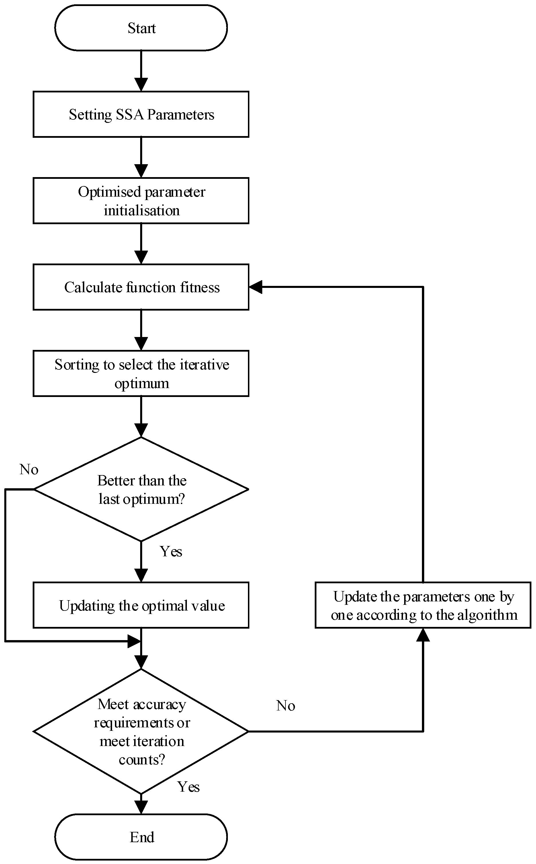
2.3.1. Sparrow Search Algorithm

Sparrow search algorithm (SSA) is mainly inspired by sparrow foraging behavior and anti-predator behavior [16]. The algorithm is parameterized by the number of iterations G, number of populations, percentage of discoverers, fitness function, and the dimension of parameters to be optimized; this indicates how many parameters need to be optimized. In this case, the CNN-BiLSTM algorithm is optimized for the number of iterations, the learning rate, the number of outputs from the convolutional layer filter, the number of hidden nodes in the BiLSTM layer, so the dimension is 4.

In this paper, SSA introduces a neural network combinatorial model; the specific calculation process is shown in Figure 4.

2.3.2. Convolutional Neural Network

CNN has a wide range of applications in image classification, recognition and prediction [17]. In the application scenario of this paper, one-dimensional time series data need to be processed. The one-dimensional convolutional computational expression is:

$$x_k^l=f({\displaystyle \sum _{i=1}^N{x}_i^{l-1}\ast {\omega }_{ik}^l+b_k^l)}$$

(18)

$x_k^l$ denotes the kth convolution of the ith layer; f is the activator; N denotes the number of convolutional mappings of the input data; $\ast$ is the convolution step; ${\omega }_{ik}^l$ is the weight of the ith operation of the kth convolution kernel of the ith layer; and $b_k^l$ is the offset of the kth convolution kernel corresponding to the ith layer.

In this paper, the maximum pooling method is used with the expression ${\widehat{x}}_k^l=\max (x_k^l:x_{k+r-1}^l)$, which is the maximum value of the vector $x_k^l$ to the vector $x_{k+r-1}^l$. The sequence x is divided into consecutive vectors with window size r. The maximum pooling operation is performed on each vector to obtain the maximum feature sequence.

2.3.3. BiLSTM Neural Network

The BiLSTM network enables each input data point to pass through the LSTM network in two directions, positive and negative, respectively, and the past and future hidden states can be recursively fed back to achieve a bidirectional loop [18]. LSTM (Long Short-Term Memory Network) successfully solves the gradient vanishing problem of RNN (Recurrent Neural Network) by employing three selective transfer mechanisms and cell state units. LSTM is able to retain the model memory of the input patterns, which overcomes the shortcomings of RNN in dealing with long-term dependency problems. This makes LSTM perform well in predictive modeling of temporal data with significant advantages for long-term memory [19,20]. In summary, LSTM has more advantages than RNN in temporal data prediction modeling, can effectively solve the long-term dependency problem, and achieve the long-term memory function.

$$\left\{\begin{array}{c}{f}_t=\sigma (W_f{x}_t+A_f{h}_{t-1}+b_f)\\ i_t=\sigma (W_i{x}_t+A_i{h}_{t-1}+b_i)\\ c_t^{’}=\tanh (W_c{x}_t+A_c{h}_{t-1}+b_c)\\ c_t=f_t\ast c_{t-1}+i_t\ast c_t^{’}\\ o_t=\sigma (W_o{x}_t+A_o{h}_{t-1}+b_o)\\ h_t=o_t\ast \tanh (c_t)\end{array}\right.$$

(19)

W_f, W_i, W_c and W_o denote the input weight vectors, while A_f,A_i, A_c and A_o denote the upper output weight vectors together with b_f, b_i, b_c and b_o denoting the bias vectors, $\sigma$ denotes the S-shape function used for gating, while the tanh function is used for generating a new storage unit cell $c_t^{’}$ due to its fast convergence.

$$\left\{\begin{array}{c}{\overrightarrow{H}}_t=LSTM(x_t,{\overrightarrow{H}}_{t-1})\\ {\overleftarrow{H}}_t=LSTM(x_t,{\overleftarrow{H}}_{t-1})\\ H_t^{’}={\alpha }_t{\overrightarrow{H}}_t+{\beta }_t{\overleftarrow{H}}_t+{\lambda }_t\end{array}\right.$$

(20)

${\overrightarrow{H}}_{t-1}$ and ${\overleftarrow{H}}_{t-1}$ are the hidden layer conditions of the LSTM network and inverse conditions at the moment $t-1$; ${\overrightarrow{H}}_t$ and ${\overleftarrow{H}}_t$ are the hidden layer conditions of the LSTM network and inverse conditions at the moment t; $\alpha$ is the forward propagation unit hidden layer output weights; $\beta$ is the backward propagation unit hidden layer output weights; $H_t^{’}$ is the total state output of BiLSTM network output, which consists of ${\overrightarrow{H}}_t$ and ${\overleftarrow{H}}_t$ hidden layer states.

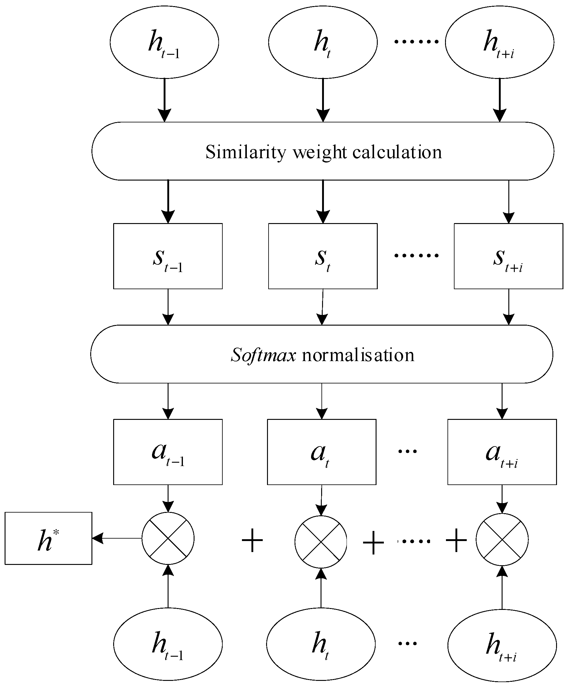
2.3.4. Attention Mechanism

The main principle of the attention mechanism is the automatic weighted average calculation [21,22]; the principle is shown in Figure 5.

$h_i$ is the output data of the implicit layer, ${\alpha }_i$ is the weight value of the input data, and $h^{\ast }$ is the final result obtained from the calculation with the following formula:

$$h^{\ast }={\displaystyle \sum _{i=1}^k{\alpha }_i{h}_i}$$

(21)

The attention mechanism uses a scoring function to calculate ${\alpha }_i$ and $h^{\ast }$. The larger the value of the scoring function, the higher the correlation. The correlation of the scoring function is calculated as $s_i$, which is the normalization function to obtain the weight value ${\alpha }_i$. Let the sum of the weight values of all $h_i$ be 1, i.e., ${\displaystyle \sum _i{\alpha }_i=1}$. The formula for ${\alpha }_i$ is shown in (22):

$${\alpha }_i=soft\max \left(s_i\right)$$

(22)

The cosine similarity method, vector dot product method and neural network method were used to evaluate the function to calculate the correlation using the following formulas:

Vector dot product method:

$$s_i=f\left(h_i,h^{\ast }\right)=h_i\cdot h^{\ast }$$

(23)

Cosine similarity methods:

$$s_i=f\left(h_i,h^{\ast }\right)={\displaystyle \frac{h_i\cdot h^{\ast }}{‖h_i‖‖h^{\ast }‖}}$$

(24)

Neural network approach:

$$s_i=f\left(h_i,h^{\ast }\right)=MLP\left(h_i\cdot h^{\ast }\right)$$

(25)

In photovoltaic power generation forecasting, the attention mechanism is able to assign the similarity weight of the PV data at each moment. The attention mechanism can capture more valuable information by assigning corresponding weights to the PV data at each moment according to its importance to the prediction results. Therefore, in order to enable BiLSTM to make full use of the differences in PV data, this paper combines BiLSTM with the attention mechanism to forecast photovoltaic power generation.

2.3.5. SSA-CNN-BiLSTM-ATT-Based Photovoltaic Power Generation Forecasting Process

The photovoltaic power generation forecast process proposed in this paper, shown in Figure 6, is mainly divided into the following steps:

(1)

Pearson’s correlation coefficient is used to analyze the actual operating data of PV arrays, determining the correlation coefficients between the variables. Heat maps are then plotted based on the correlation coefficients to visualize the relationships between the variables.

(2)

Fuzzy C-means cluster analysis classifies the historical photovoltaic power generation sequence samples into three categories: sunny weather changes, cloudy weather changes, and rainy weather changes.

(3)

To identify the optimal component parameter k, the historical PV power generation sequence undergoes decomposition. Variational modal decomposition is applied to each weather type, assuming k modal components exist for slow weather conditions.

(4)

Empirical direct observation divides the k modal components derived from step (3) into high-frequency and low-frequency components.

(5)

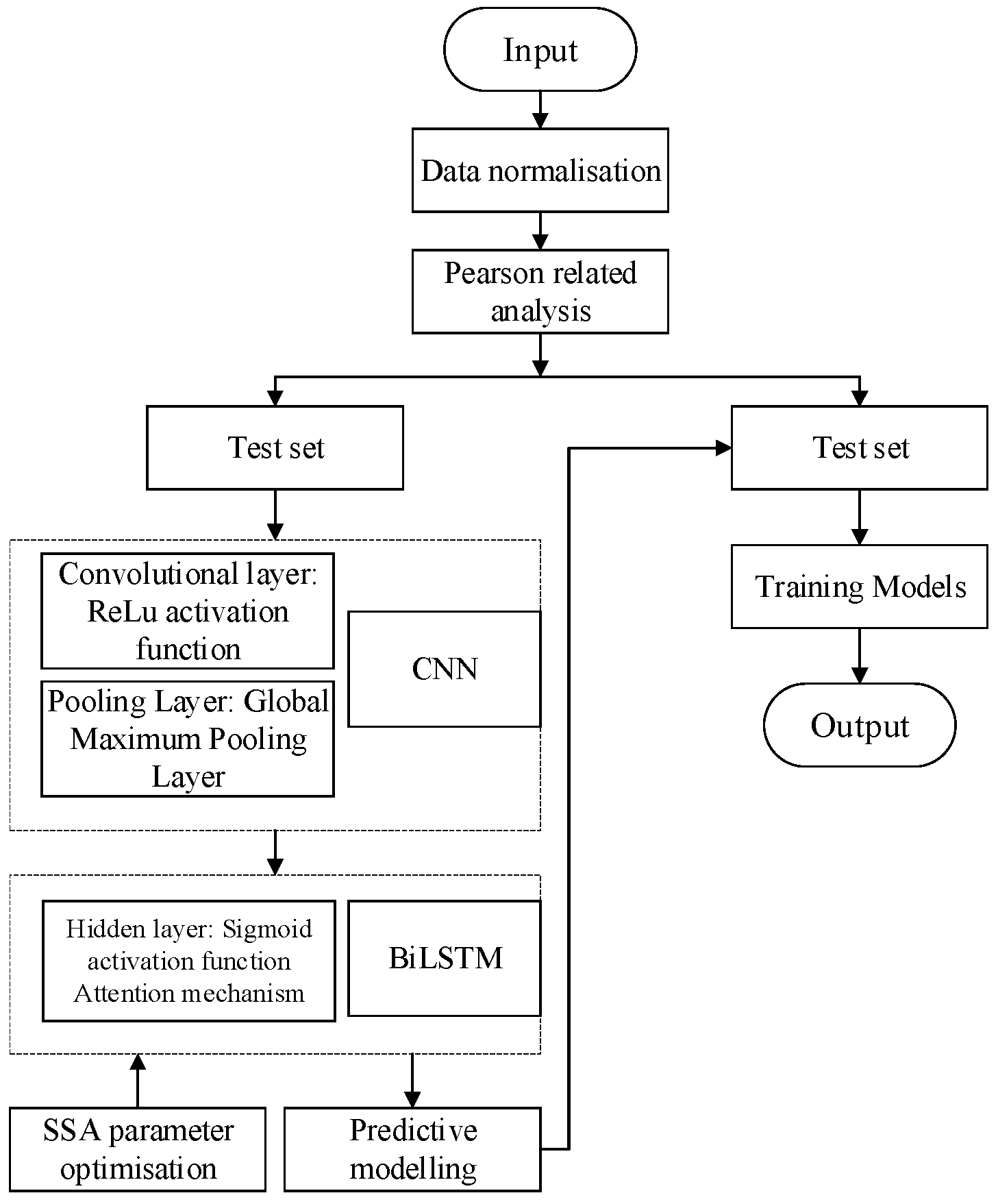
A two-layer prediction framework is designed. A CNN model is used for the low-frequency part, and a BiLSTM model is used for the high-frequency part. In order to improve the model performance, the model parameters are optimized using the improved sparrow algorithm, and the attention mechanism is introduced so that the model can pay more attention to the key features.

(6)

By feeding real-time environmental data into the trained neural network, the model predicts the high-frequency and low-frequency components separately and combines the predictions to arrive at the predicted value of PV power generation.

2.4. Evaluation of Photovoltaic Power Generation Forecasting Models

2.4.1. Mechanism Analysis of Photovoltaic Power Generation Prediction Error Generation

The PV power prediction process is composed of three links: input data, prediction model, and result processing. Among them, the input data and the prediction model will generate errors. The errors in the input data are mainly from the forecasting errors in Numerical Weather Prediction (NWP), mainly due to the following reasons:

(1)

The NWP model is a time- as well as space-discretized continuum time-space method, which is bound to have some errors.

(2)

There are anomalies in the observed data, which will further generate errors when assimilated into the NWP model.

(3)

The atmospheric system is very complex, and the use of partial differential equations to describe its system is highly sensitive to the existence of errors in the initial conditions, but the errors will gradually accumulate with the passage of time.

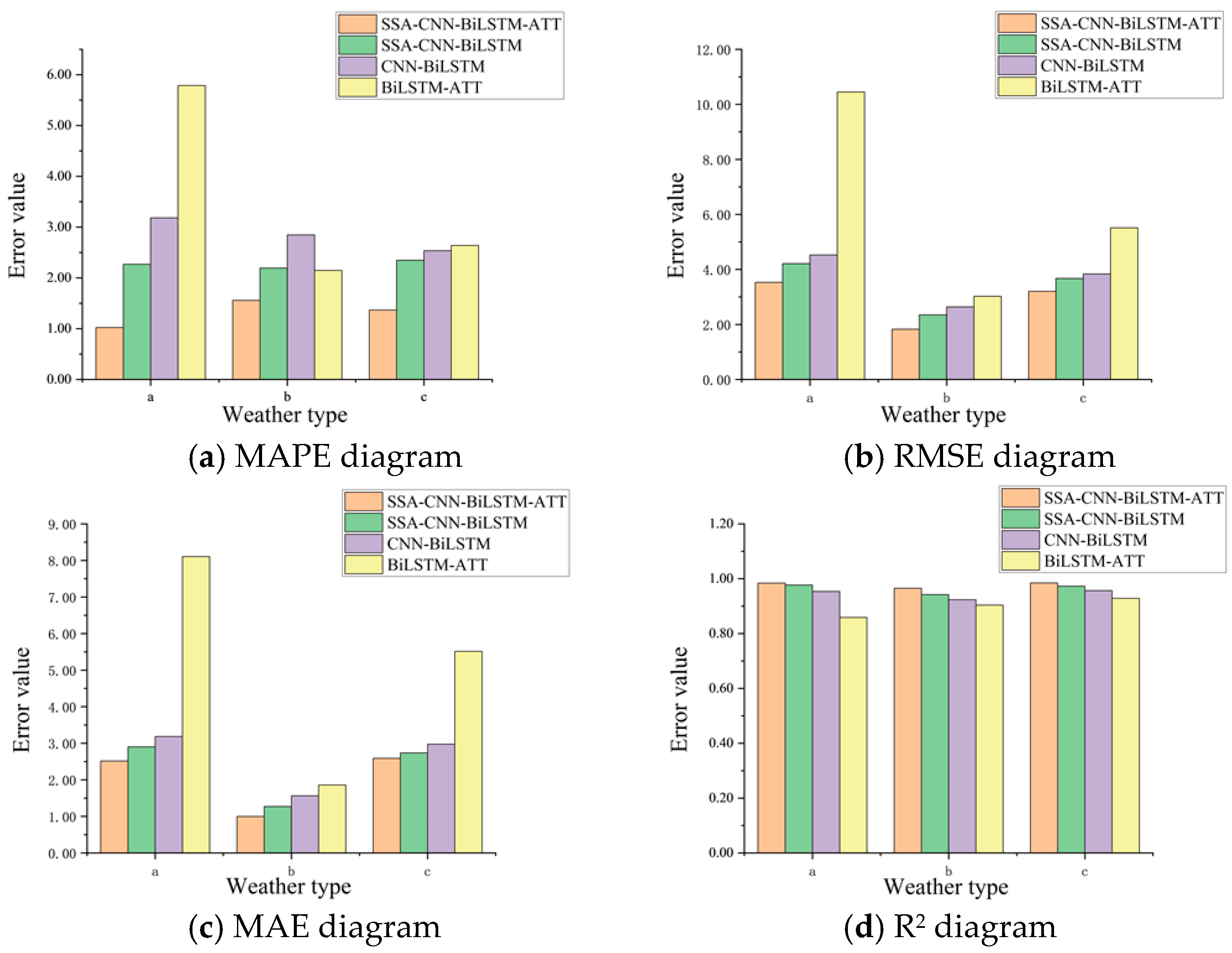
2.4.2. Indicators for Evaluating Projected Results

The performance of the photovoltaic power generation forecast model is quantitatively analyzed by choosing the error assessment indices with reference to science [23]. The prediction accuracy of the prediction model was tested by using MAPE and RMSE. MAPE can evaluate the prediction ability of the prediction model, and RMSE can evaluate the degree of dispersion of the prediction model, and also, the average absolute error MAE and R-Squared can be used as the prediction model evaluation index in this paper. The specific formulas are, respectively:

$$MAPE={\displaystyle \frac{1}{N}}{\displaystyle \sum _{j=1}^N\frac{\left|h_t-{h_t}^{’}\right|}{{h_t}^{’}}}\times 100\%$$

(26)

$$RMSE=\sqrt{{\displaystyle \frac{1}{N}}{\displaystyle \sum _{j=1}^N{(h_t-{h_t}^{’})}^2}}$$

(27)

$$MAE={\displaystyle \frac{1}{N}}{\displaystyle \sum _{j=1}^N\left|h_t-{h_t}^{’}\right|}$$

(28)

$$R^2=1-{\displaystyle \frac{{\displaystyle \sum _{j=1}^n{(h_t-{h_t}^{’})}^2}}{{\displaystyle \sum _{j=1}^n{({h_t}^{’}-h_t)}^2}}}$$

(29)

The real and expected generation of solar power at time t is denoted by $h_t$ and ${h_t}^{’}$, respectively, and N is the number of samples.

3. Distributed Power Scheduling Model for Microgrids

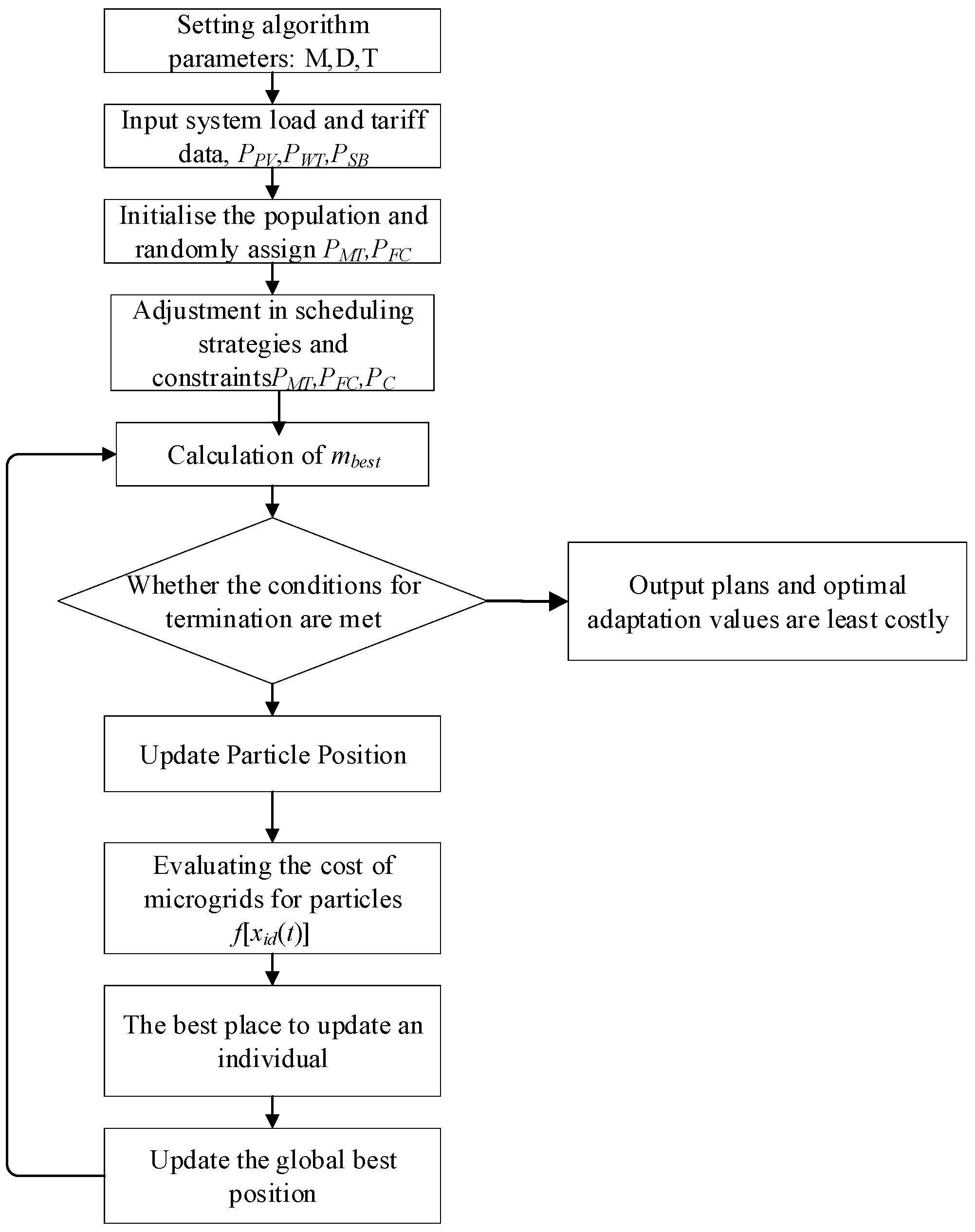
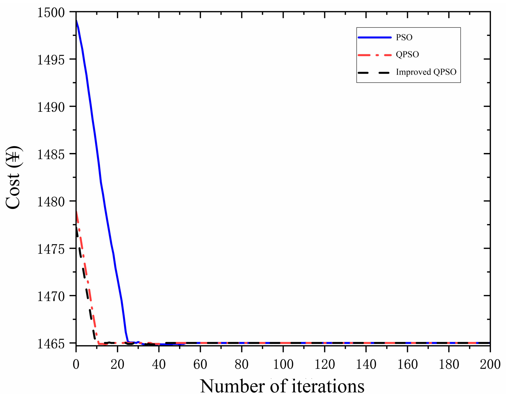
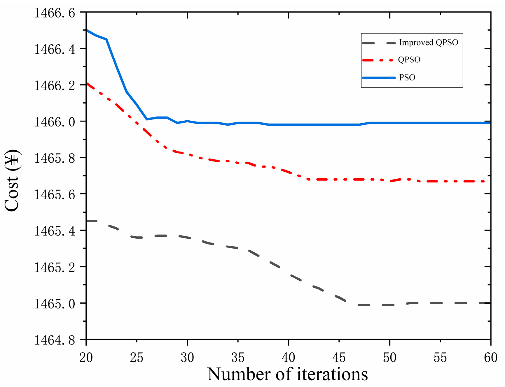
3.1. Improved Quantum Particle Swarm Algorithms

Quantum particle swarm optimization (QPSO) is based on the principle of quantum mechanics and improves the search efficiency by using the position and velocity information of particles [24]. However, QPSO often struggles to escape the local optimal solution during the optimization process, especially in the later stages, resulting in limited overall performance [25]. To overcome this problem, the idea of differential evolution is introduced in QPSO. Differential evolution effectively optimizes the solution of the problem through competition and collaboration among individuals, enabling the algorithm to better explore the global optimal solution space. The introduction of differential evolution allows each individual to adjust its position by exchanging information with other individuals, thus increasing the probability of jumping out of the local optimal solution. By combining the idea of differential evolution, the improved QPSO not only overcomes the limitations of the later stages, but also significantly improves the overall optimization ability, making it perform better in solving complex optimization problems. As a result, the improved QPSO performs more efficiently and reliably in realizing the global optimal solution, showing stronger adaptability and robustness.

The flow of the improved QPSO algorithm is shown in Figure 7.

3.2. Microgrid Scheduling Model

3.2.1. Scheduling Model

A microgrid is a small power system consisting of a variety of decentralized distributed energy sources, such as wind power, photovoltaics, and fuel cells. In this study, the distributed generator is selected as a distributed energy system consisting of wind turbine, photovoltaic, microturbine, fuel cell and battery.

(1)

Objective function

The objective of microgrid economic and environmental scheduling is to minimize the comprehensive cost. Under the premise of satisfying the normal operation of each microgrid power source, their outputs are reasonably arranged. For microgrids, in order to ensure that the system operates efficiently while minimizing negative impacts on the environment, it is necessary to find a balance between costs and benefits.

$$C_{sum}=C_1+C_2$$

(30)

C₁ is the operating cost, including fuel cost, maintenance cost, depreciation cost; in addition, there is a need for a comprehensive assessment of the costs incurred by microgrids in buying power from and selling power to the main grid. C₂ is the environmental cost, i.e., the cost of dealing with polluted gases.

$$\begin{array}{l}{C}_1={\displaystyle \sum _{H=1}^T{\displaystyle \sum _{i=1}^N(\Delta T{C}_i^{CG}(H)+\Delta T{K}_i{P}_i(H)+{\displaystyle \sum _{i=1}^N\frac{AD{C}_i}{P_{i,\max }a{f}_i}{P}_i(H)}}}\\ +{\displaystyle \sum _{H=1}^T\Delta T{P}_c}(H)C_{grid}(H)+{\displaystyle \sum _{H=1}^T\Delta T{K}_{bat}}\left|P_{bat}(H)\right|)\end{array}$$

(31)

T is the microgrid operation period; N is the number of controllable elements; $\Delta T$ is time period; $C_i^{CG}$ is the fuel cost of unit i in period H; $K_i$ is the maintenance cost of unit i; $P_i(H)$ is the output of unit i in period H; $a$ is a constant; $AD{C}_i$ is the annual depreciation cost of unit i; $f_i$ is the capacity factor; $P_c\left(H\right)$ is the purchased and sold power from the main grid and the microgrid in period H; $P_{bat}(H)$ is the charging and discharging power of the battery in period H; and $K_{bat}$ is the charging and discharging cost of the battery in period H.

The components of environmental costs are listed below:

$$C_2={\displaystyle \sum _{k=1}^K{\alpha }_k{\lambda }_{k1}{P}_{MT}(H)}+{\displaystyle \sum _{k=1}^K{\alpha }_k{\lambda }_{k2}{P}_{FC}(H)}+{\displaystyle \sum _{k=1}^K{\alpha }_k{\lambda }_{k3}CGP(H)}$$

(32)

${\alpha }_k$ is the external discounted cost of type k emissions; ${\lambda }_{kn}$ is the emission factor, with 1, 2, and 3 denoting Micro Turbine, Fuel Cell, and the main microgrid, respectively; K is the type of emission (NOx, SO2, or CO2); PMT(H) and PFC(H) are the output power, respectively, at H.

Table 3. External discounted cost and emission factor.

Typology	External Discount Cost (CNY/kg)	Emission Factor (kg/MW)
		Micro Turbine	Fuel Cell	Primary Network
$N{O}_x$	8.00	0.2	0.014	1.6
$S{O}_2$	6.00	0.0036	0.0027	1.8
$C{O}_2$	0.023	724	489	889

summarizes the external discounted costs and emission factors based on publicly available data from local governments.

The relevant parameter settings for each unit in the microgrid system are shown in

Table 4. Operating unit parameters.

Module Type	Wind Turbine	Photovoltaic	Micro Turbine	Fuel Cell	Storage Battery
Installation cost (CNY/kW)	23,750.00	66,500.00	18,500.00	52,710.00	—
Maintenance cost factor	0.02941	0.00962	0.00963	0.02911	0.0452
Depreciation cost factor	0.71	2.793	0.0111	0.251	—
Upper limit power (kW)	10.00	10.00	65.00	40.00	20.00
Life span (years)	10.00	20.00	15.00	10.00	5.00

.

(2)

Binding conditions

Battery capacity limitation constraints:

$$-20\le P_{SB}\le 20$$

(33)

Battery charging and discharging limits:

$$P_{bat}(H)=P_{dis}(H)-P_{ch}(H)$$

(34)

$$0\le P_{dis}(H)\le P_{dis},\max (H)\times U_{dis}(H)$$

(35)

$$0\le P_{ch}(H)\le P_{ch},\max (H)\times U_{ch}(H)$$

(36)

$$U_{dis}(H)+U_{ch}(H)=1$$

(37)

$${\displaystyle \sum _{i=1}^T\left|U_{ch}(H)-U_{ch}(H-1)\right|}\le N_{bat}$$

(38)

The energy balance constrains the battery at the beginning and end of the period:

$${\displaystyle \sum _{i=1}^T{P}_{bat}(H)=0}$$

(39)

P_SB is the output of the battery, $P_{dis}(H)$ and $P_{ch}(H)$ are the discharging power and charging power of the battery in H-cycle, respectively; $U_{dis}(H)$ and $U_{ch}(H)$ denote the state of the battery in H-cycle, respectively, with 1 being the charging state and 0 being the discharging state; $P_{dis}$, $\max (H)$ are the upper limit of the discharging power and the upper limit of the charging power of the battery in H-time period; $N_{bat}$ is the upper limit of the battery’s charging and discharging times; and $P_{bat}(H)$ is the algebraic sum of battery charging and discharging power.

Output Limits:

$$P_i,\min (H)\le P_i(H)\le P_i,\max (H)$$

(40)

Constraints on the rate of climb:

$$-R_i^{down}\Delta T\le P_i^{CG}(H)-P_i^{CG}(H-1)\le R_i^{up}\Delta T$$

(41)

CG is the amount of power generated by the controllable unit; $P_{i,\min }^{CG}$ and $P_{i,\max }^{CG}$ are the limits of the output of the unit i, respectively; and $R_i^{down}$ and $R_i^{up}$ are the downward and upward climb rates of the unit i, respectively.

System constraints:

$${\displaystyle \sum _{i=1}^N{P}_i^{CG}(H)}+{\displaystyle \sum _{i=1}^M{P}_i^{RG}(H)}+P_C(H)=P_L(H)$$

(42)

RG is the renewable unit power generation; $P_C(H)$ is the microgrid power purchase and sale; power is sold to the main grid for $P_C(H)>0$ and purchased from the main grid for $P_C(H)<0$; and $P_L(H)$ denotes the load of the microgrid system.

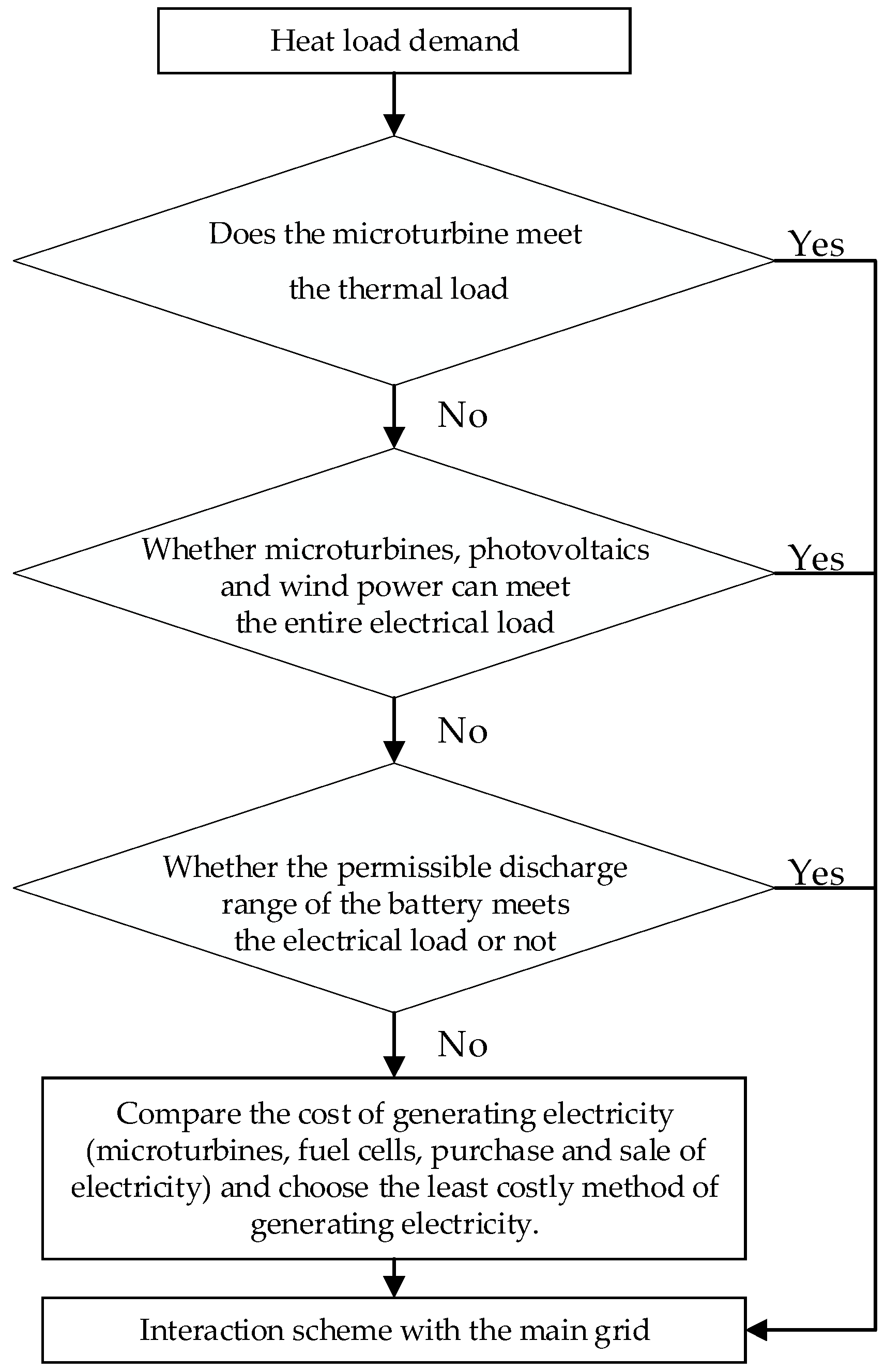
3.2.2. Dispatch Strategy

Distributed generators in microgrids usually use renewable energy sources, whereas distributed generators in conventional grids use energy sources such as fuel generators. In view of the above characteristics of microgrid energy, this paper proposes the following strategies. Wind turbine power generation should first satisfy the winter heat load, and then satisfy the small electrical load if necessary. When microturbine, PV and wind power generation cannot satisfy the full electrical load, the algorithm proposed in this paper will allow the batteries to be discharged progressively under high load conditions to avoid system overload and to satisfy the load demand. The algorithm will consider selling the power to the main grid. If the electrical load cannot be met within the allowable discharge range of the battery, the algorithm will perform a cost comparison. After comparing the cost of fuel cell power generation, micro-turbine power generation and power trading, the algorithm will choose the less costly option to supply power or interact with the main grid. The specific decision-making process is shown in Figure 8.

Based on the basic data, this paper obtains the cost curves of power generation from microturbines and fuel cells through MATLAB R2021a, as shown in Figure 9 and Figure 10. After comparing the cost of fuel power generation, microturbine power generation and electric power business, the power generation method is determined. The specific analyses are shown in

Table 5. Comparative cost analysis.

Phase	Cost Comparisons	Analysis
Low periods of electricity consumption	$C_{FCJ}>C_{BUY},C_{SALE}$	Fuel cells do not generate electricity
	$C_{MTJ}>C_{BUY},C_{SALE}$	Microturbines do not generate electricity after encountering thermal loads
Flat periods of electricity consumption	$C_{SALE}<C_{FCJ}<C_{BUY}$	Fuel cells do not generate electricity after encountering an electrical load
	$C_{MTJ}>C_{BUY},C_{SALE}$	Microturbines do not generate electricity after encountering thermal loads
Peak periods of electricity consumption	$C_{FCJ}<C_{BUY},C_{SALE}$	Fuel cell full power generation
	$C_{MTJ}<48>C_{BUY},C_{SALE}$	Microturbines do not generate electricity after encountering thermal loads
	$C_{SALE}<C_{MTJ}>48<C_{BUY}$	Micro-turbine power generation to meet electrical loads

.

In the following operation, it will rely mainly on the battery for charging and discharging management. If the electrical load demand of the system and the charging demand of the batteries cannot be met, the microgrid will purchase power from the main grid to compensate for the shortfall. Conversely, when the microgrid generates more power than it needs, the excess power will be sold to the main grid.

(1)

Low periods of electricity consumption

In microgrid systems, the cost of generating electricity from microturbines and batteries is usually higher than the price of purchasing electricity directly from the grid, within their allowable output. In such cases, microturbines and batteries are not used for power generation. The primary function of the batteries is to meet the electrical load of the microgrid and ensure its proper operation. However, when the batteries cannot meet the demand, the microgrid needs to purchase electricity from the main grid. In order to ensure the economy and sustainability of microgrids, the operational efficiency of microturbines and storage batteries must be optimized to achieve the best cost of power generation and energy utilization efficiency. Therefore, optimizing the operational efficiency of these devices is crucial for the long-term viability of microgrids.

(2)

Flat periods of electricity consumption

In a microgrid system, the cost of generating electricity from batteries is lower than the price of purchasing electricity, although it is higher than the price of selling electricity in the range of its output power. Therefore, the system prioritizes the use of battery discharge to meet the electrical demand. If the electrical load exceeds the discharge capacity of the batteries or the batteries are in a state of charge, the fuel cells will start generating electricity. When the fuel cell is also unable to meet the demand, the microgrid will purchase power from the main grid. In summary, when the microgrid operates, the system prioritizes the use of battery discharge to meet the demand, and if it is insufficient, the fuel cell will be activated, and finally, the power will be purchased from the main grid to ensure the economy and reliability of the system.

(3)

Peak periods of electricity consumption

In microgrid systems, the cost of generating electricity from fuel cells is always lower than the price of purchasing and selling electricity, making them a cost-effective option in all cases. In contrast, the generation cost of a micro gas turbine depends on the magnitude of its output power. When the output power is lower than 48 kW, the cost of electricity generated by MGTs is higher than the cost of purchasing electricity from the grid, and thus not economical, while when the output power is higher than 48 kW, the cost of electricity generated is lower than the cost of purchasing electricity, and thus becomes economical. The 48 kW threshold becomes a key equilibrium point for MGTs, which determines the threshold of their economic performance. Based on the characteristics of this balance point, the micro gas turbine generates electricity only when its output power exceeds 48 kW to satisfy the electrical load demand and the battery charging demand. At the same time, in order to maintain the economy and efficiency of the system, the micro gas turbine does not sell excess power to the main grid in this case, but focuses on meeting internal demand.

Taken together, the microgrid system is able to achieve the best economic efficiency under different power demands by rationally utilizing fuel cells and micro gas turbines. Among them, fuel cells show high economy and efficiency under all circumstances due to their generation costs, which are always lower than the prices of purchased and sold electricity, while micro gas turbines optimize their operating costs and benefits by generating electricity when the output power exceeds 48 kW, thus providing a flexible and economical generation option for micro grids. It can be seen that microgrids are able to realize the economy and efficiency of energy supply under different load conditions through scientific and reasonable equipment scheduling and power management.

4. Practical Case Studies

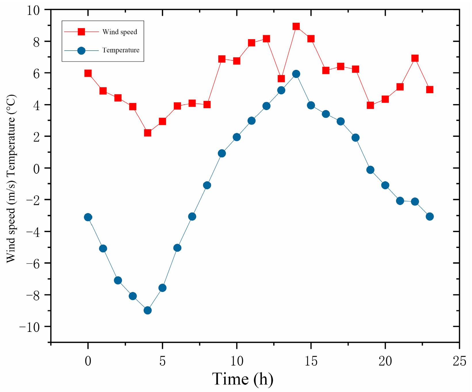
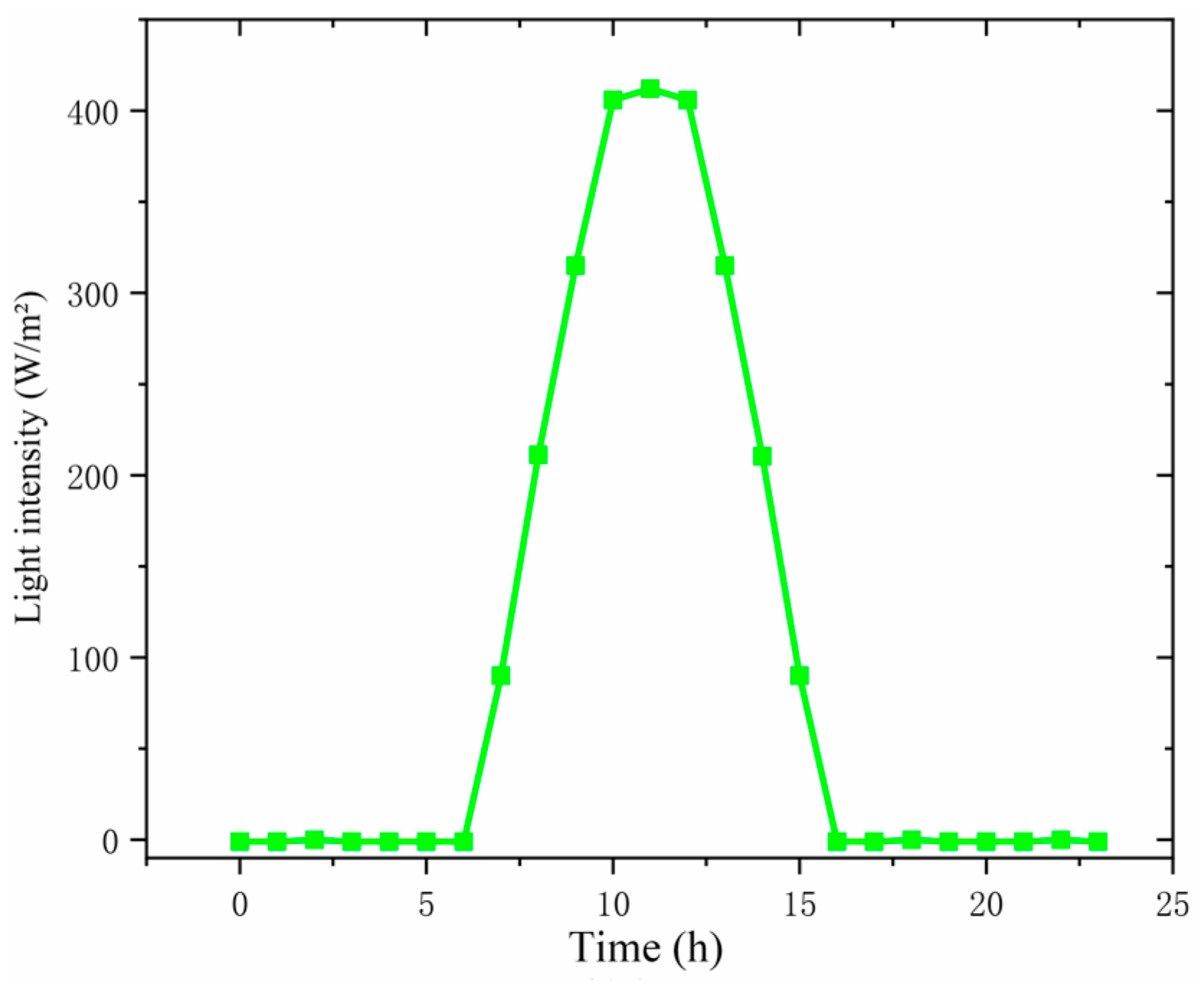
4.1. Example Simulation of Photovoltaic Power Generation Prediction

In this paper, we select the public typical environmental data of a city in China, a photovoltaic power generation forecast for the period between January 2020 and December 2020, and the solar performance data characteristics obtained through the above screening, with a temporal resolution of 15 min, which is chosen for comparison with other photovoltaic power generation forecasting methods in this paper.

Because photovoltaic power is not generated by the photovoltaic system at night, the 0 power in the nighttime data is deleted from it, and the data are stored between 6:00 and 19:00 every day for analysis. In this paper, first, PV data are processed using principal component analysis and cluster analysis algorithm, and secondly, the Pearson correlation coefficient is used to analyze the filtered data, and the samples are input into the CNN-BiLSTM network, and the parameters are determined after several rounds of training. And in this paper, we will optimize the number of neurons, and using the SSA algorithm, Figure 11 shows the fitness curve of the SSA algorithm-optimized CNN-BiLSTM model compared with other algorithms. The number of convolutional kernels is 32 and 64 with a step size of 2. All data are filtered and spread through a pooling layer.

Input the processed data, then select three typical days: sunny, complex weather and rainy days, as prediction days and validate the accuracy of the prediction model using MAPE, RMSE, MAE and R² as the evaluation metrics of the model.

The following computer configurations were applied in the case study: Python 4.0, TensorFlow 2.7.0 programming, processor Intel (R) Core (TM) i7-7700HQ (Santa Clara, CA, USA), and simulation software PyCharm 2022.2.3. The implementation of SSA-CNN-BiLSTM short-term photovoltaic power generation forecast is based on the attention mechanism.

In this section, the SSA-CNN-BiLSTM-Attention neural network based on SSA-CNN-BiLSTM-Attention neural network will be used to forecast photovoltaic power generation forecast for the next 500 data points, and to compare the effectiveness of the SSA-CNN-BiLSTM-ATT model proposed in this paper, the SSA-CNN-BiLSTM Optimization Algorithm model, the CNN-BiLSTM Combined Neural Network model, and the BiLSTM- ATT model, to verify the effectiveness of the proposed model in this paper. Figure 12 shows the iterative curve of different algorithms’ function fitness values, from which it can be seen that the combined algorithm proposed in this paper has higher accuracy and convergence speed than other algorithms.

In this paper, the model parameters are investigated, and after many trials and adjustments, this paper comes up with the optimal hyperparameter settings, as shown in

Table 6. Parameter settings.

Typology	Parameters
Activation function	ReLU function
Number of iterations	50
Learning rate	0.001
Fine-tuning learning rate	0.1
Regularization parameter	0.5

.

Table 7. The value of each model hyperparameter.

Modelling	Number of Iterations	Population size	Learning Rate	Hidden Node 1, 2	Fully Connected Node
CNN-BiLSTM	50	20	0.001	10	10
BiLSTM-ATT	60	10	0.001	10	10
SSA-CNN-BiLSTM	100	20	0.001	10	10
SSA-CNN-BiLSTM-ATT	150	20	0.002	10	20

shows the hyperparameter values for each model, including num epochs (number of iterations), batch size, Lr (learning rate), and Fc (number of nodes in the fully connected layer). In CNN-BiLSTM, SSA-CNN-BiLSTM-ATT, and SSA-CNN-BiLSTM prediction models, hidden1 and hidden2 represent the hidden nodes in the BiLSTM layers, respectively; in LSTM models, hidden1 and hidden2 represent the first and second hidden nodes in the first and second layers, respectively,; in the BiLSTM-Attention model, hidden1 and hidden2 represent the hidden nodes in the first and second BiLSTM layers, respectively; and in the SSA-CNN-BiLSTM-Attention prediction model, there are two more hyperparameters, i.e., the size of CNN convolutional kernels size is 3. The values of these hyperparameters are obtained by iterative testing and tuning.

The training set data are imported into the power generation prediction network to obtain the initial measurement data and error series, and the SSA-CNN-BiLSTM-ATT network is built to predict the errors, and the final prediction results are obtained by summing the predicted results. The prediction results of three typical weather days are selected according to the clustering results and compared with the prediction results of SSA-CNN-BiLSTM, CNN-BiLSTM and BiLSTM-ATT. Class a is sunny days, class b is complex days, and class c is rainy days, and the comparison of the errors of different models for the three different weather types is shown in

Table 8. Error result of prediction model.

Error Parameter	Weather Types	SSA-CNN-BiLSTM-ATT	SSA-CNN-BiLSTM	CNN-BiLSTM	BiLSTM-ATT
MAPE	a	1.0225	2.2689	3.1825	5.7866
	b	1.5562	2.1935	2.8462	2.1464
	c	1.3673	2.3472	2.5347	2.6372
RMSE	a	3.5292	4.2110	4.5231	8.4481
	b	1.8258	2.3490	2.6374	3.0254
	c	3.2021	3.6725	3.8354	5.5128
MAE	a	2.5150	2.9021	3.1852	8.1065
	b	0.9986	1.2703	1.5632	1.8591
	c	2.5876	2.7354	2.9756	5.5128
R2	a	0.9839	0.9770	0.9536	0.8586
	b	0.9650	0.9420	0.9235	0.9038
	c	0.9845	0.9728	0.9568	0.9286

, in order to visually represent the prediction accuracy of this paper’s algorithms.

The data in Table 8 show that the BiLSTM-ATT neural network has the worst prediction effect; its RMSE is as high as 10.4481, and R² values are all minimum values. SSA-CNN-BiLSTM-ATT prediction model has the best performance, its RMSE in the three weather categories are 3.5292, 1.8258, and 3.2021, and its R² values are 0.9839, 0.9650, and 0.9845, with the lowest MAPE and MAE. SSA-CNN-BiLSTM-ATT has the smallest MAPE and MAE among the models compared to SSA-CNN-BiLSTM, CNN-BiLSTM, and BiLSTM-ATT, with the highest improvement in RMSE of 5.8%, and an increase in R² of 1.27%, respectively (Figure 13).

From the above analysis, it can be seen that the first three models predict better in sunny weather, but in complex weather and rainy weather conditions, the prediction effect of the SSA-CNN-BiLSTM-ATT prediction model proposed in this paper is obviously due to the other prediction models.

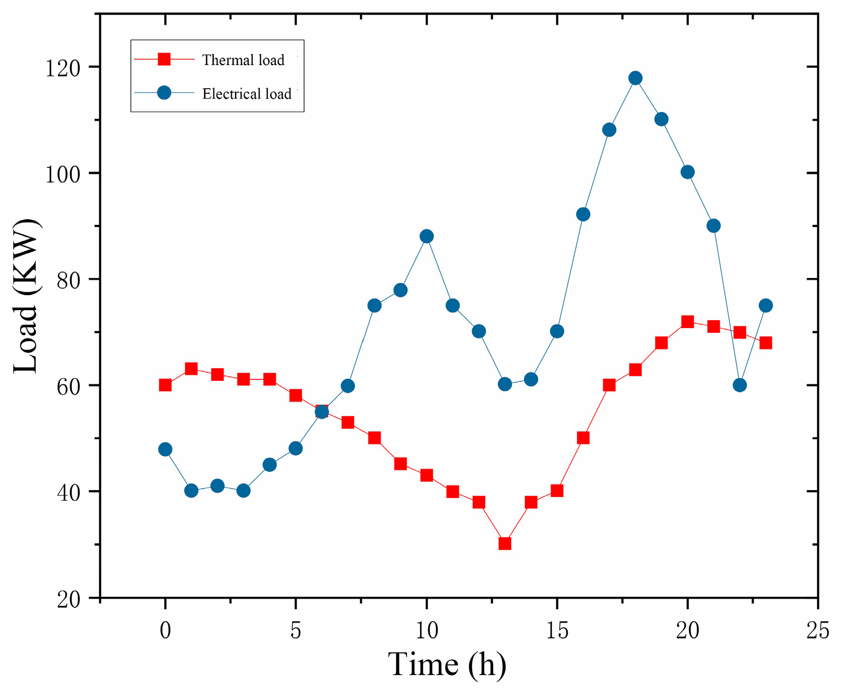
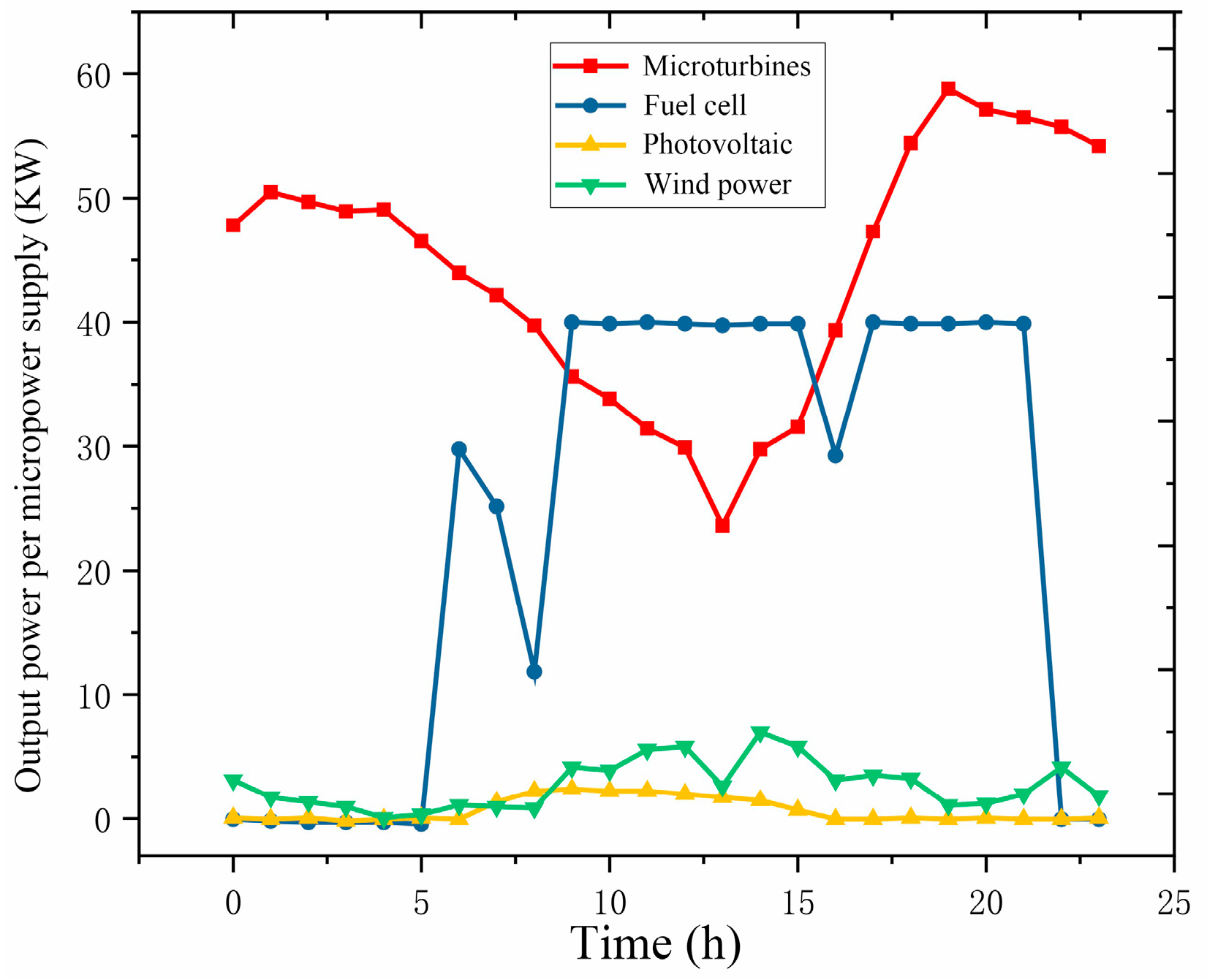
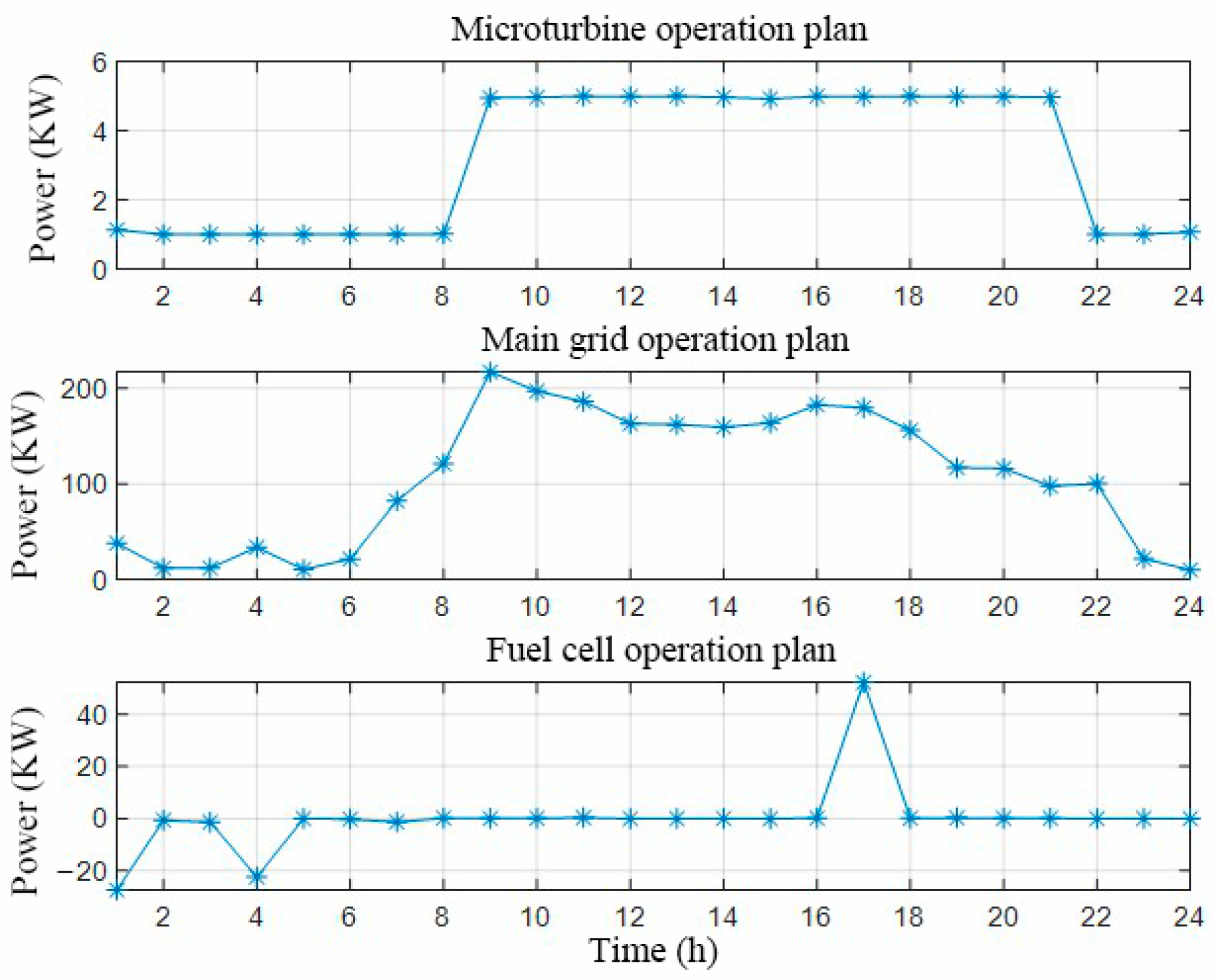
4.2. Simulation of a Microgrid Distributed Energy Dispatch Example

The microgrid modelled in this paper specifically includes microturbine power generation (65 kw), photovoltaic power generation (10 kw), fuel cell (40 kw), wind turbine power generation (10 kw), and storage battery (20 kw). The loads in the case of this paper include residential loads and industrial loads, and the scheduling time is 1 day and the unit time interval is 1 h. The microgrid power system of this paper is shown in Figure 14.

The data related to the cases in this paper are shown in Figure 15, Figure 16 and Figure 17.

Table 9. Electricity price levels at different points in time.

Mode	Period	Tariff Price (CNY/kWh)
Electricity purchase	Peak period (10:30–14:30, 18:30–20:30)	0.83
	Regular period (7:30–9:30, 15:30–17:30, 21:30–22:30)	0.49
	Bottom period (23:30–06:30)	0.17
Electricity sale	Peak period (10:30–14:30, 18:30–20:30)	0.65
	Regular period (7:30–9:30, 15:30–17:30, 21:30–22:30)	0.38
	Bottom period (23:30–06:30)	0.13

shows the data of purchased and sold electricity prices in different periods.

Based on the micro-power system operation strategy above, the output of each micro-power source on a typical winter day as well as the purchased and sold power of the micro-grid can be known, as shown in Figure 18. Figure 18 shows the power curve of each micro power source for 24 h. Because winter is the heating period, the micro turbine first generates electricity to meet the heat load, and from Figure 18, it can be seen that the micro turbine can satisfy the heat load of a typical day in winter within the range of the output power. Then, wind and photovoltaic power generation are fully utilized, and when the power supply is still insufficient to meet the electrical load, battery and fuel cell generation, subsequent generation from the microturbine, or the purchase of power from the main grid are considered to meet the load.

Figure 19 shows a scheme of how the microgrid interacts with the main grid, which is divided into the following three time periods:

(1)

Low periods of electricity consumption (23:30–06:30)

Between 1:30 and 4:30, microturbine’s output exceeds thermal load requirements, causing battery discharge and excess power sold to the main grid. From 5:30 to 6:30, combined microturbine, battery, wind, and photovoltaic generation surpasses the thermal load, but is insufficient to charge batteries, necessitating grid power purchase. Between 23:30 and 00:30, the microturbine, wind, and photovoltaic output falls short of electrical load, requiring battery recharge.

(2)

Flat periods of electricity consumption (07:30–09:30, 15:30–17:30, 21:30–22:30)

At 07:30, 08:30, 09:30, and 17:30, the combined output from wind, fuel cell, and microturbine precisely matches electrical load and battery power requirements, eliminating the need for grid power sales. Conversely, at 15:30, 16:30, 21:30, and 22:30, sole fuel cell generation proves insufficient to meet electrical load and battery charging demands, necessitating grid power purchase.

(3)

Peak periods of electricity consumption (10:30–14:30, 18:30–20:30)

In the microgrid system, the generation and power demand at different time periods are as follows. At 10:30, 11:30, 12:30, and 18:30, the fuel cells fully generate power, the batteries are discharged, and the microgrid sells excess power to the main grid. At 13:30 and 14:30, although the fuel cells are generating at full capacity, the total generation from the units is still insufficient, and the microgrid needs to purchase power from the main grid to make up the shortfall. At 19:30 and 20:30 in the evening, the fuel cells do not generate enough power and the microturbine meets the heat load demand after generating more than 48kW. In summary, the microgrid balances the power demand and supply through the synergistic operation of fuel cells and microturbines, as well as the purchase or sale of power, depending on the time period and load conditions.

In this study, we compare the performance of three algorithms, namely, improved QPSO, standard QPSO and PSO, on the economic and environmental scheduling problem of microgrids. Some of the parameter settings of the three algorithms were kept consistent to ensure the accuracy of the comparison results. The study was conducted for 230 iterations and the cost was recorded every five generations to obtain a total of 41 datasets. Subsequently, the differences in the costs of the three algorithms were analyzed using Friedman’s test with the initial assumption that there is no significant difference in scheduling costs among the three algorithms. The actual running results are shown in

Table 10. Friedman test results.

Name of Algorithm	Average Rankings
PSO	2.85
QPSO	2.02
Improved QPSO	1.12

. Through iterative and statistical tests, this study analyzes the performance difference between the improved QPSO and the other two algorithms in terms of microgrid scheduling cost.

The initial and late performance of these three algorithms is analyzed based on the above results.

Figure 20 shows that the PSO algorithm has the highest sensitivity to the initial data and the remaining two algorithms have relatively low sensitivity to the initial data. The standard deviation is derived by calculating the cost data from generation 1–20 and the results are as follows. Standard QPSO is 13.4775, PSO is 4.9380, and improved QPSO is 5.8169. This indicates that in the pre-iteration period, the PSO algorithm has the least volatility and performs the most consistently, improved QPSO is the second most volatile, and standard QPSO has the most volatility and the highest sensitivity to the initial data. It is concluded that the PSO algorithm performs the most stably in the pre-iteration period, the improved QPSO is second and the standard QPSO has the largest volatility.

From

Table 11. Algorithm iteration result.

Number of Iterations	Improved QPSO	QPSO	PSO
1	1478.53	1496.1404	1499.975
5	1475.13	1492.835	1497.8886
10	1470.49	1477.8428	1494.6328
15	1465.49	1467.2558	1489.274
20	1465.43	1466.5655	1489.0882
25	1465.4	1466.0593	1488.829
30	1465.38	1466.3064	1488.7039
35	1465.37	1466.30439	1488.6686
40	1465.32	1466.3038	1488.6327
45	1465.24	1466.3037	1488.5629
50	1465.08	1466.3037	1488.5631
55	1464.97	1466.3037	1488.5631
60–230 (stable value)	1464.97	1466.3037	1488.5631

and Figure 21, it can be concluded that the standard Quantum Particle Swarm Optimization (QPSO) algorithm tends to stabilize at generation 34, while the Particle Swarm Optimization (PSO) algorithm reaches a steady state at generation 45. However, the improved QPSO algorithm only stabilizes in generation 52 and is still actively searching for an optimal solution at this stage. This performance suggests that the improved QPSO algorithm has a greater ability to better disengage from the local optimal solution and successfully enter the global optimal solution at a later stage.

Figure 21 shows the convergence points for three sets of data, 1466.0037 (standard QPSO), 1465.6831 (PSO), and 1464.9660 (improved QPSO). These data further demonstrate that the improved QPSO algorithm is capable of obtaining better solutions with better convergence results than the standard QPSO and PSO algorithms. This performance improvement not only proves the significant advantages of the improved QPSO in algorithm optimization, but also demonstrates its efficiency and reliability in dealing with complex system problems.

The improved QPSO algorithm performs more rationally and efficiently in the environmental and economic operation of microgrid systems. This improvement allows the QPSO algorithm to better balance the energy production and consumption of the system during the optimization of microgrids, reducing energy consumption and operating costs while improving environmental benefits. By adopting the improved QPSO algorithm, the microgrid system can realize the optimal economic and environmental operation status and give full play to its role in sustainable development.

Overall, the improved QPSO algorithm performs more effectively than the standard QPSO and PSO algorithms in solving the microgrid scheduling problem. It not only has a significant improvement in optimization efficiency and accuracy, but also shows superiority in economy and environmental protection. The improved QPSO has broad prospects for future microgrid applications and provides strong support and a new approach for the optimization of microgrid systems.

5. Conclusions

Accurate PV power forecasting is essential for improving the reliability of microgrid power systems, ensuring safe and stable operation, and achieving economic dispatch. This paper proposes an SSA-CNN-BiLSTM-Attention model to enhance prediction accuracy through step-by-step optimization of data preprocessing, model construction, and training. The model considers the operating characteristics of distributed power sources, establishes an economic and environmental protection model for microgrids, and uses an improved QPSO algorithm to solve the microgrid power generation scheduling problem. Test results demonstrate that the combined SSA-CNN-BiLSTM-Attention neural network outperforms other algorithms in prediction accuracy, while the improved QPSO algorithm effectively addresses the scheduling problem with a focus on economic and environmental goals. However, there are still areas for improvement. Future research could incorporate spatial correlation analysis of neighboring power stations to further enhance prediction accuracy, address the challenges of the SSA-CNN-BiLSTM-Attention model under complex weather conditions, and expand to the economic and environmental scheduling of multiple microgrids, exploring more efficient optimization methods to improve algorithm performance and accuracy.

References

1. Cao, R.; Tian, H.; Li, D.; Feng, M.; Fan, H. Short-Term Photovoltaic Power Generation Prediction Model Based on Improved Data Decomposition and Time Convolution Network. Energies 2023, 17, 33. [Google Scholar] [CrossRef]
2. Abdellatif, A.; Mubarak, H.; Ahmad, S.; Ahmed, T.; Shafiullah, G.M.; Hammoudeh, A.; Abdellatef, H.; Rahman, M.M.; Gheni, H.M. Forecasting Photovoltaic Power Generation with a Stacking Ensemble Model. Sustainability 2022, 14, 11083. [Google Scholar] [CrossRef]
3. Wei, X.; Wang, M. Research on Data Model and Integration Technology of New Energy Power System. In Proceedings of the 2017 4th International Conference on Information Science and Control Engineering (ICISCE), Changsha, China, 21–23 July 2017; pp. 1135–1139. [Google Scholar] [CrossRef]
4. Leva, S.; Dolara, A. Analysis and Vlidation of 24 Hours Ahead Neural Network Forecasting of Photovoltaic Output Power. Math. Comput. Simul. 2017, 131, 1325–1340. [Google Scholar] [CrossRef]
5. Tan, Z.; De, G.; Li, M. Combined Electricity Heat-cooling-gas Load Forecasting Model for Integrated Energy System Based on Multi-task Learning and Least Square Support Vector Machine. Clean. Prod. 2020, 248, 119252–119263. [Google Scholar] [CrossRef]
6. Aslam, S.; Herodotou, H.; Mohsin, S.M. A Survey on Deep Learning Methods for Power Load and Renewable Energy Forecasting in Smart Microgrids. Renew. Sustain. Energy Rev. 2021, 144, 524–536. [Google Scholar] [CrossRef]
7. Kim, M.K.; Kim, Y.-S. Predictions of Electricity Consumption in a Campus Building Using Occupant Rates and Weather Elements with Sensitivity Analysis: Artificial Neural Network vs. Linear Regression. Sustain. Cities Soc. 2020, 62, 515–530. [Google Scholar] [CrossRef]
8. Kalliola, J.; Kapočiūtė-Dzikienė, J.; Damaševičius, R. Neural Network Hyperparameter Optimization for Prediction of Real Estate Prices in Helsinki. PeerJ Comput. Sci. 2021, 7, 434–444. [Google Scholar] [CrossRef] [PubMed]
9. Zhou, T.; Hu, Q.; Hu, Z. An Adaptive Hyper Parameter Tuning Model for Ship Fuel Consumption Prediction under Complex Maritime Environments. J. Ocean. Eng. Sci. 2021, 5, 260–265. [Google Scholar] [CrossRef]
10. Netsanet, S.; Zheng, D.; Zhang, W.; Teshager, G. Short-Term PV Power Forecasting Using Variational Mode Decomposition Integrated with Ant Colony Optimization and Neural Network. Energy Rep. 2022, 10, 8. [Google Scholar] [CrossRef]
11. Liang, L.; Su, T.; Gao, Y.; Qin, F.; Pan, M. FCDT-IWBOA-LSSVR: An Innovative Hybrid Machine Learning Approach for Efficient Prediction of Short-To-Mid-Term Photovoltaic Generation. J. Clean. Prod. 2023, 385, 135716. [Google Scholar] [CrossRef]
12. Dhiman, G. MOSHEPO: A Hybrid Multi-Objective Approach to Solve Economic Load Dispatch and Micro Grid Problems. Appl. Intell. 2020, 50, 119–137. [Google Scholar] [CrossRef]
13. Prasad, T.N.; Devakirubakaran, S.; Muthubalaji, S.; Srinivasan, S.; Kamel, S. Power Management in Hybrid ANFIS PID Based AC–DC Microgrids with EHO Based Cost Optimized Droop Control Strategy. Energy Rep. 2022, 8, 15081–15094. [Google Scholar] [CrossRef]
14. Luo, S.; Guo, X. Multi-Objective Optimization of Multi-Microgrid Power Dispatch under Uncertainties Using Interval Optimization. J. Ind. Manag. Optim. 2023, 19, 823–851. [Google Scholar] [CrossRef]
15. Li, S.; Chen, X.; Yin, L.; Zhang, F.; Wu, P.; Zhao, S.T. Evaluation and Research of Photovoltaic Power Generation Model Considering Climate Change. Acta Energiae Solaris Sin. 2022, 43, 79–84. [Google Scholar] [CrossRef]
16. Peng, O.; Ren, T.; Wang, Y. Short-term Wind Power Prediction by Optimizing Deep Learning Network Hyper-Parameters Based on ISSA. Smart Power 2023, 51, 31–38+52. [Google Scholar]
17. Huang, X.; Li, Q.; Tai, Y.; Chen, Z.; Liu, J.; Shi, J.; Liu, W. Time series forecasting for hourly photovoltaic power using conditional generative adversarial network and Bi-LSTM. Energy 2022, 246, 123403. [Google Scholar] [CrossRef]
18. Kim, T.Y.; Cho, S.B. Predicting residential energy consumption using CNN-LSTM neural networks. Energy 2019, 182, 72–81. [Google Scholar] [CrossRef]
19. Zhang, X.; Shang, J.; Yu, G. Bearing Fault Diagnosis Based on Attention for Multi-Scale Convolutional Neural Network [J/OL]. J. Jilin Univ. Eng. Technol. Ed. 2023, 1–10. [Google Scholar] [CrossRef]
20. Yao, Z.; Lu, Z.; Li, C. Improved CEEMDAN-PSO-BiLSTM Model for Short-term Passenger Flow Prediction at Bus Stops. J. Beijing Jiaotong Univ. 2023, 47, 74–80. [Google Scholar]
21. Sun, H.; Li, F. Photovoltaic Hot Spot Recognition Based on Attention Mechanism. Acta Electron. Sin. 2023, 44, 453–459. [Google Scholar] [CrossRef]
22. Zhou, H.; Bai, H.; Cai, Z. Container Quota Optimization Algorithm Based on GRNN and LSTM. Acta Electron. Sin. 2022, 50, 366–373. [Google Scholar]
23. Qu, W.; Chen, G.; Zhang, T. An adaptive noise reduction approach for remaining useful life prediction of lithium-ion batteries. Energies 2022, 15, 7422. [Google Scholar] [CrossRef]
24. Kang, L.; Zhang, X.; Oleg, K. SLSL-QPSO: Quantum-behaved particle swarm optimization with short-lived swarm layers. SoftwareX 2023, 24, 101536. [Google Scholar] [CrossRef]
25. Zhu, X.T.; Xu, B. Power short-term load forecasting based on QPSO-SVM. Adv. Mater. Res. 2012, 591, 1311–1314. [Google Scholar] [CrossRef]
Figure 1. Heat map of correlation coefficient of each variable.
Sustainability 17 00648 g001
Figure 2. Data clustering result graph.
Sustainability 17 00648 g002
Figure 3. Data preprocessing flow chart.
Sustainability 17 00648 g003
Figure 4. Flow chart of optimization parameters of SSA algorithm.
Sustainability 17 00648 g004
Figure 5. Structure diagram of attention mechanism.
Sustainability 17 00648 g005
Figure 6. Flow chart of photovoltaic power generation prediction model based on SSA-CNN-BiLSTM-ATT.
Sustainability 17 00648 g006
Figure 7. Improved QPSO flowchart.
Sustainability 17 00648 g007
Figure 8. Microgrid scheduling strategy.
Sustainability 17 00648 g008
Figure 9. Microturbine power cost curve.
Sustainability 17 00648 g009
Figure 10. Fuel cell generation cost curve.
Sustainability 17 00648 g010
Figure 11. The fitness curve of CNN-BiLSTM-ATT prediction model was optimized by different algorithms.
Sustainability 17 00648 g011
Figure 12. Convergence diagram of different algorithms.
Sustainability 17 00648 g012
Figure 13. Bar chart of error for different weather types under different forecast models.
Sustainability 17 00648 g013
Figure 14. Microgrid power system.
Sustainability 17 00648 g014
Figure 15. Daily heat load and electricity load in winter.
Sustainability 17 00648 g015
Figure 16. Winter daily wind speed and temperature.
Sustainability 17 00648 g016
Figure 17. Winter light intensity.
Sustainability 17 00648 g017
Figure 18. Curve of microgrid generation.
Sustainability 17 00648 g018
Figure 19. Microgrid interaction curve.
Sustainability 17 00648 g019
Figure 20. Performance comparison of algorithms.
Sustainability 17 00648 g020
Figure 21. Comparison of algorithms in the later stage.
Sustainability 17 00648 g021