Hydrothermal Coupling Analysis of Frozen Soil Temperature Field in Stage of Pipe Roof Freezing Method

Abstract

Taking the Sanya River Mouth Channel project as a case study, this research explores the minimum brine temperature required for the pipe-jacking freezing method during staged freezing. Based on the heat transfer theory of porous media, a three-dimensional model of the actual working conditions was established using COMSOL 6.1 finite element software. By adjusting the brine cooling scheme, the development and distribution patterns of the freezing curtain under different brine temperatures were analyzed. The results indicate that as the staged freezing brine temperature increases, the thickness of the freezing curtain decreases linearly, and the closure of isotherms is inhibited. When the brine temperature is −8 °C, the thickness of the freezing curtain meets the minimum requirement and effectively achieves the freezing effect under both low and high seepage flow conditions. Additionally, seepage significantly affects the formation of the freezing curtain, causing it to shift towards the direction of seepage, with the degree of shift becoming more pronounced as the seepage velocity increases. When the seepage velocity is so high that the thickness of the freezing curtain on one side is less than 2 m, the impact of seepage on the freezing curtain can be reduced by decreasing the hydraulic head difference in the freezing area or by increasing the arrangement of freezing pipes, thereby enhancing the freezing effect.

1. Introduction

The excavation of coastal tunnels with large cross-sections often encounters the impact of groundwater, and there are frequent cases of leakage due to groundwater seepage in the project. To prevent major engineering accidents caused by groundwater seepage, the trench curtain method has been introduced into the project [1]. The pipe curtain method is particularly superior for underground engineering with shallow burial depth, large cross-section, and complex geology [2]. The curtain method, despite its development, has been limited by its poor water stoppage properties, which has allowed the artificial ground freezing method [3] to gain widespread use in tunnel engineering due to its superior water stoppage capabilities [4]. Scholars have combined the curtain method and the artificial ground freezing method to create a new technique known as the curtain freezing method. This method was first applied in the dark-excavation tunnels in the construction of the Gongbei Tunnel for the Hong Kong-Zhuhai-Macao Bridge Connecting Line [5,6,7]. In this method, the grouting curtain support structure serves as the main load-bearing system, fully utilizing the tensile strength of the steel pipes [8]. The artificial ground freezing technique freezes the soil to form a frozen curtain, which acts as a water stop component [4]. This method makes full use of the waterproofing, homogeneity, and recoverability of frozen soil, ensuring the stability and safety of the overall tunnel structure [9].

As an excellent construction method, many scholars in China have conducted research on the curtain freezing method, which has been applied in various tunnel projects, demonstrating its effectiveness and practicality. Duan et al. used the Hong Kong-Zhuhai-Macao Bridge Gongbei Tunnel as a case study to establish a two-dimensional finite element calculation model that considers the freezing-tunnel-bedrock freezing temperature field. Through comparisons with field observation data, they studied the development patterns of the frozen curtain and the changes in frost heave displacement during the freezing period [10]. Hu et al. [11] developed a freezing control system to solve the problem of soil sealing for long-distance top-down tunnelling. They conducted in situ tests to explore the optimal freezing scheme and control mode. Qi et al. [12] explored the application of the artificial ground freezing method in large underground engineering projects in cities. They analyzed the formation and development of the freezing mass when multiple freezing pipes work together, revealing the synergistic effects observed during the freezing process. They proposed the basin-shaped freezing method. The study by Ou et al., which addresses the heave and subsidence of the ground surface caused by soil freeze-thaw cycles, has developed a series of numerical models for frozen ground. This research can be used to test the deformation of the foundation caused by the AGF method and the impact of the thickness of the freezing wall on the AGF method [13]. Hu et al. [14] applied the artificial ground freezing method in shield tunnels, linking the freezing area with the freezing time. They studied the horizontal freezing method for soil reinforcement in shield driven tunnels, proving the feasibility of the artificial ground freezing method in shield tunnels. Huang et al. [15] aimed to achieve safety and energy efficiency by constructing a water-heat coupled model to simulate the influence of groundwater flow on the freezing process. They combined this model with the Nelder-Mead Simplex method based on the COMSOL Multiphysics platform to optimize the positions of freezing pipes around circular tunnels.

The above studies did not consider the need for substantial resource supply in actual engineering to achieve the purpose of saline water cooling using the pipe curtain freezing method. In order to advocate resource conservation, environmental protection, and low-carbon policies, as well as to provide engineering guidance for the Sanya River Estuary Channel project, it is necessary to study the impact of adjusting the saline water cooling plan during the freezing stage on the temperature field. This paper uses the pipe curtain freezing engineering project of the Sanya River Estuary Channel, using the COMSOL finite element software for analysis. Different saline water cooling plans will be selected for comparison, and the most energy-efficient saline water cooling temperature will be explored. Additionally, the temperature will be compared under different seepage conditions, providing theoretical reference for the design and construction of future pipe curtain freezing engineering.

2. Project Background

2.1. Overview

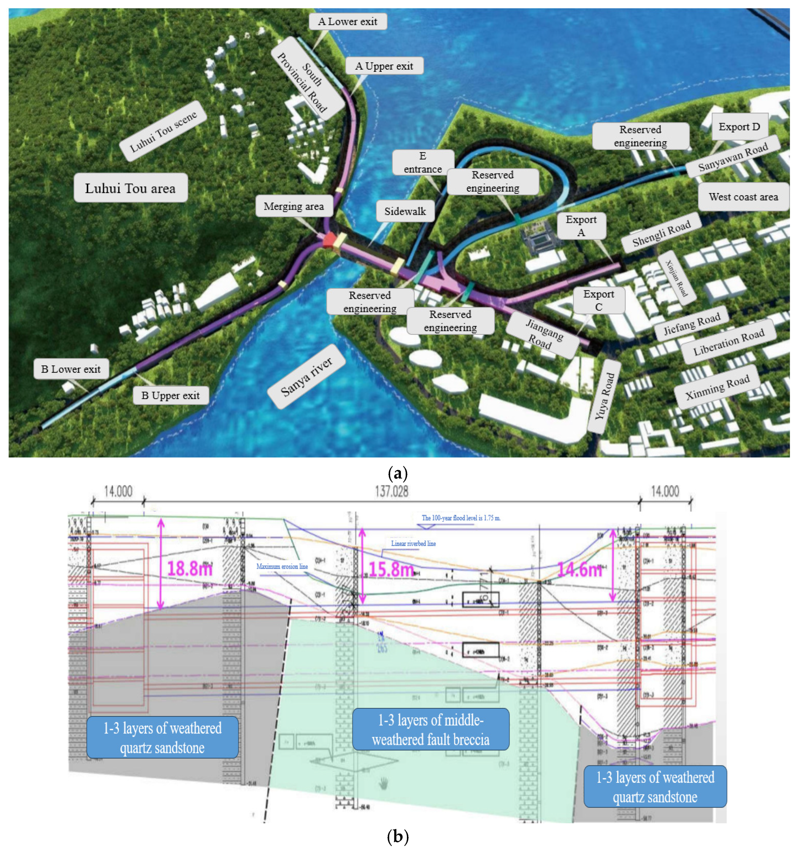
The Sanya River Estuary Channel project is located in Tianya District, Sanya City. As an important link connecting Luhui Tou Peninsula, the project is of great significance in enhancing economic development, perfecting urban road networks, and alleviating traffic pressure. The two banks of the project are constructed using open excavation methods. The design depth of the work pit on the west bank is about 28 m, and the design depth of the work pit on the Luhui Tou side is about 29 m. The tunnel is 3180 m long and is designed as a single-hole double-layer structure stacked in layers. It crosses the Sanya River estuary, as shown in Figure 1a. The tunnel passes through layers of soil from top to bottom, including fine sand, coral debris, strong quartz sandstone, and medium quartz sandstone, as shown in Figure 1b. The complex geological conditions and various unfavorable soil layers pose challenges to the project. Ordinary curtain methods are difficult to ensure effective water stoppage due to the complex geological conditions. Therefore, the curtain freezing method is used.

2.2. Scheme Design of Freezing Pipe Curtain Method

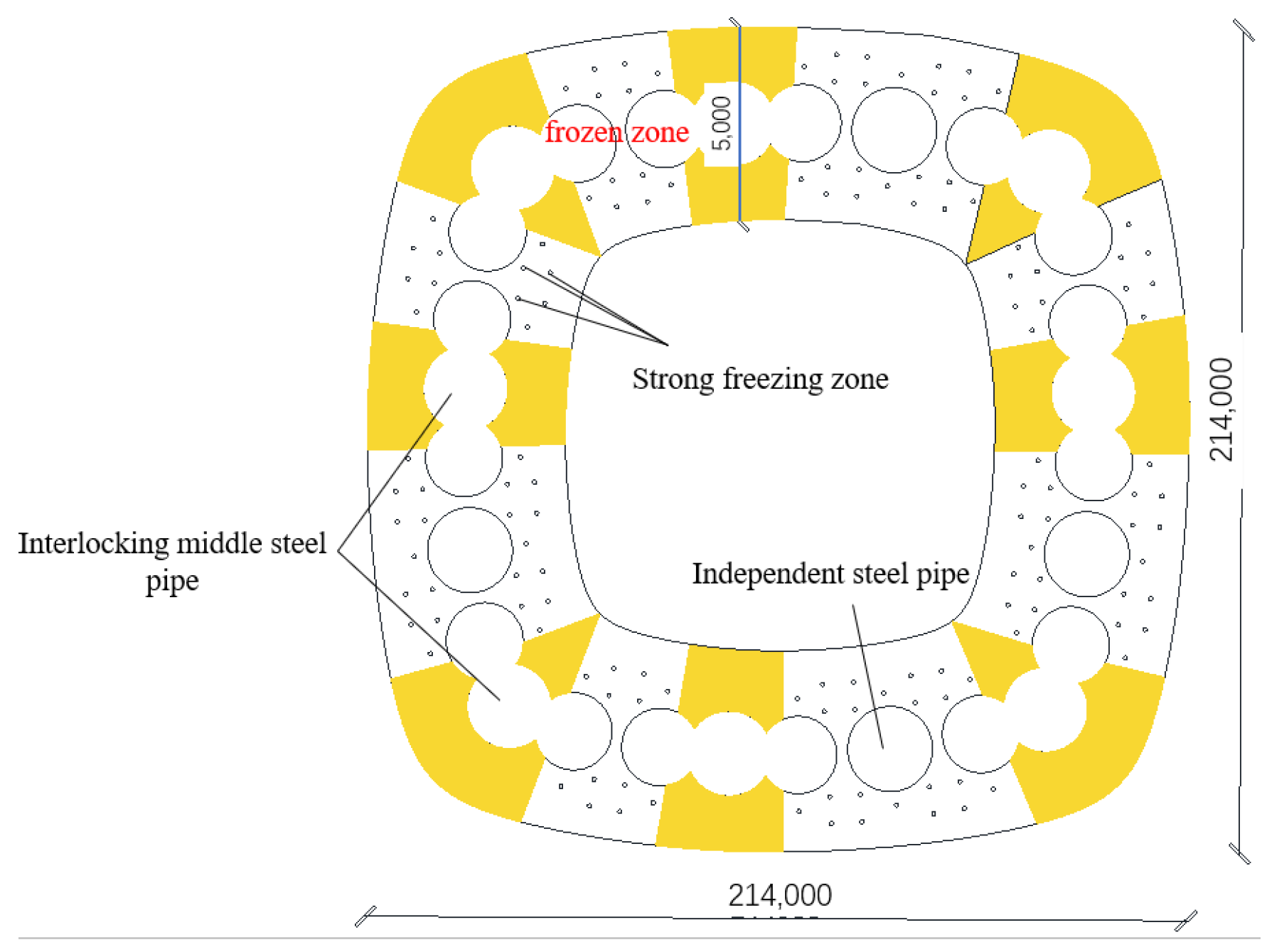
The text describes a tunnel freezing method construction technique where 28 pipes are arranged around the tunnel to form a pipe curtain. Out of these, eight groups consist of three pipes each, forming interlocking pipes. The middle pipe in each group has a diameter of 2100 mm, while the side pipes have a diameter of 2000 mm. Additionally, there are 4 independent pipes with a diameter of 2200 mm. Also, there are circular freezing pipes buried in the soil with a diameter of 108 mm. The freeze protection pipes are arranged in an inner and outer ring pattern using 136 pipes. The freezing area is divided into strong and weak freezing zones. The strong freezing zone is distributed around the inner and outer sides of the pipe seam at the connection of the interlocking pipes, while the weak freezing zone refers to the inner and outer sides of the interlocking pipes. The arrangement of the freeze protection pipes and the pipes is shown in Figure 2.

3. Numerical Modeling and Computational Theory

3.1. Thermal Field Theory

The freezing process of soil is governed by heat conduction theory, where heat is transferred from a high-temperature medium to a low-temperature medium, and the soil interacts with the low-temperature medium in the freeze protection pipes to form frozen soil, solidifying the water in the soil. The heat conduction in porous media is related to the factors of fluid flow [16]. The heat conduction equation in the temperature field under fluid flow conditions is as follows:

$${\left(\rho C\right)}_{eff}{\displaystyle \frac{\partial T}{\partial t}}+{\rho }_f{C}_{fu}·\mathsf{\nabla }T+\mathsf{\nabla }·\left(-k_{eff\mathsf{\nabla }}\mathsf{\nabla }T\right)=Q$$

(1)

$${\left(\rho C\right)}_{eff}=={\theta }_{s{\rho }_{{sC}_s}}+\left(1-{\theta }_S\right){\rho }_{{fC}_f}$$

(2)

In the equation, the subscripts S and f represent the solid and fluid, respectively; ρ is the density, with units of ${\mathrm{k}\mathrm{g}·\mathrm{m}}^{-3}$; C is the specific heat capacity, with units of $\mathrm{J}·{\mathrm{k}\mathrm{g}}^{-1}·{\mathrm{K}}^{-1}$; ∇ is the Hamiltonian operator; T is the temperature, with units of K; u is the convective velocity, with units of $\mathrm{m}·{\mathrm{d}}^{-1}$; Q is the other heat source and sink term; $k_{eff}$ is the effective thermal conductivity, with units of $\mathrm{W}·{\mathrm{m}}^{-1}·{\mathrm{K}}^{-1}$; and ${\theta }_s$ is the solid volume fraction.

3.2. Theory of Seepage Field

Fluid flow in porous media is often laminar or near-laminar, which is suitable for Darcy’s law. The formula for Darcy’s law is as follows:

$${\displaystyle \frac{\partial }{{\partial }_t}}\left(ϵ\rho \right)+\mathsf{\nabla }·\left(\rho u\right)=Q_m$$

(3)

$$u=-{\displaystyle \frac{K}{\eta }}\mathsf{\nabla }{\rm P}$$

(4)

In the equation, the subscript t represents time, with units of d; ∇ is the Hamiltonian operator; ∇P is the pressure gradient; $Q_m$ is the source term; u is the Darcy flow velocity, with units of ${\mathrm{m}·\mathrm{d}}^{-1}$; K is the permeability of the soil, with units of ${\mathrm{m}}^2$; η is the viscosity of water; and ρ is the density of water, with units of ${\mathrm{k}\mathrm{g}·\mathrm{m}}^{-3}$.

4. Establishing a Numerical Model

4.1. Geometry Model Construction

COMSOL is a multi-physical field simulation software that allows users to simulate and analyze a variety of physical phenomena, and seepage analysis is one of them. In practical engineering, the cross-sectional dimensions of the pipe curtain freezing support structure are approximately 21.4 m × 21.4 m. Considering that there may be errors in the boundary model, the three-dimensional model dimensions are set to 30 m (length) × 30 m (height) × 10 m (width). The COMSOL software is used for finite element analysis, and the three-dimensional model and network division diagram are shown in Figure 3.

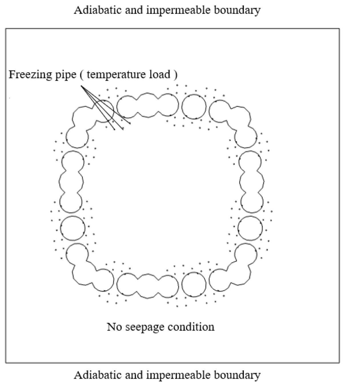
The model is set to adiabatic and impermeable on all three directions of length, width, and height. The fluid flow is set to no flow conditions. The boundary conditions are set as shown in Figure 4.

4.2. Parameter Selection

When studying the temperature field [17], it involves various parameters such as porosity, density, thermal conductivity, specific heat capacity, etc., for water, ice, sand, and frozen soil [18]. Assumptions:

• The soil layer within the freezing area is a saturated sandy layer, which is continuous, homogeneous, and isotropic.
• The fluid flow field in the freezing area satisfies Darcy’s law, and the flow velocity is zero after freezing.
• The influence of the stress field on the temperature field is not considered; only the coupling effect of the temperature field and the fluid flow field is considered.
• Freezing curtain can be formed stably and firmly within the −10 °C isotherm area.

Through experimental studies [19], various parameters are obtained, as shown in

Table 1. Physical parameters of materials.

Material	Density $\left(\mathbf{K}\mathbf{g}·{\mathbf{m}}^{-3}\right)$	Specific Heat Capacity $\left(\mathbf{W}·{\left(\mathbf{m}·\mathbf{K}\right)}^{-1}\right)$	Thermal Conductivity $\left(\mathbf{J}·{\left(\mathbf{k}\mathbf{g}·\mathbf{K}\right)}^{-1}\right)$	Permeability Coefficient $\left(\mathbf{m}·{\mathbf{s}}^{-1}\right)$
Water	1000	4180	0.55	-
Ice	920	2100	2.14	-
Soil	1990	1063	2.37	2.70 × 10−6
Frozen soil	1890	720	2.47	1.96 × 10−30

:

4.3. Cooling Schedule

This study initially adopts the staged freezing method by adjusting the saltwater cooling plan, initially setting the freezing plan to 60 days, and starting the staged freezing plan 10 days later. The saltwater temperature is adjusted to −30 °C from 23 h a day to the next day at 7 h, and from 7 to 23 h, it is −20 °C, −10 °C, −8 °C, and −5 °C, respectively. Detailed information can be found in

Table 2. Salt water cooling plan.

Time	Temperature
0	−18
10	−30 (23~7 h)
	−20, −10, −8, −15 (7~23 h)
20	−30 (23~7 h)
	−20, −10, −8, −15 (7~23 h)
30	−30 (23~7 h)
	−20, −10, −8, −15 (7~23 h)
40	−30 (23~7 h)
	−20, −10, −8, −15 (7~23 h)
50	−30 (23~7 h)
	−20, −10, −8, −15 (7~23 h)
60	−30 (23~7 h)
	−20, −10, −8, −15 (7~23 h)

.

4.4. Path Selection

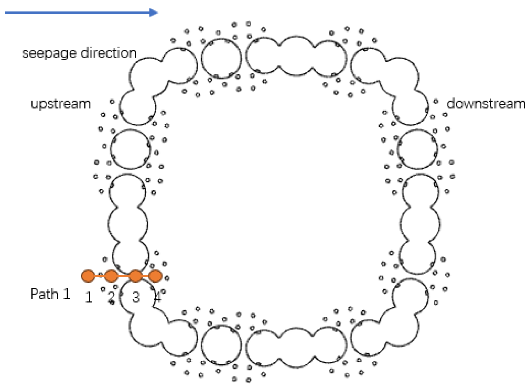
To better compare the thickness of the freezing curtain formed and the change in the cooling curve of the frozen soil under different saline water cooling plans, a path and four observation points along the path are set up. Each observation point is 100 mm apart, and the distribution of the path observation points is shown in Figure 5.

5. Simulation Results Analysis

The water head difference between the upper and lower parts of the model is set to ∆H = 0 m, which corresponds to no fluid flow conditions. To better understand the overall development of the freezing curtain, a location in the weak freezing zone is selected. By comparing and analyzing the thickness of the freezing curtain formed at different saline water temperatures at 20 d, 40 d, and 60 d, and the development trend of the isotherms, the requirements for freezing can be judged.

5.1. Freezing Curtain Comparison Analysis

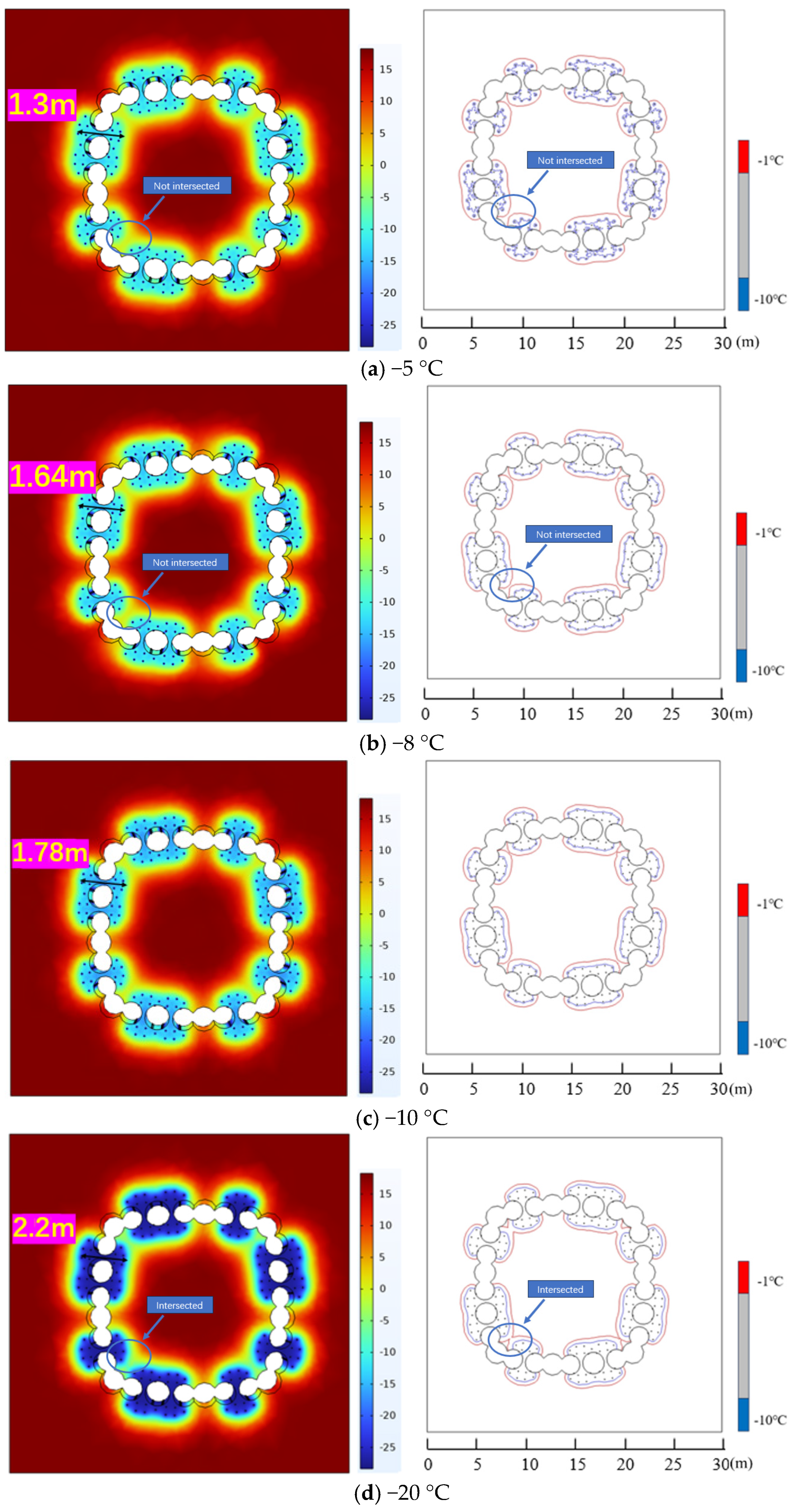
Figure 6 presents the temperature field cloud map and isotherms after 20 days of staged freezing. As illustrated in Figure 6, at 20 days of freezing, the thickness of the freezing curtain formed by saline water at −5 °C is only 1.3 m, which falls short of the required minimum thickness of 2 m. At −8 °C and −10 °C, the thicknesses of the freezing curtains are 1.64 meters and 1.78 meters, respectively, which also do not meet the requirement. However, at −20 °C, the thickness of the freezing curtain reaches 2.2 m, satisfying the requirement for a freezing curtain with a thickness of at least 2 m. It can be concluded that during the staged freezing process, lower saline water temperatures lead to a faster formation of the freezing curtain.

Comparing the isotherms at each saline water temperature reveals the following: At a saline water temperature of −5 °C, the −1 °C isotherm begins to form, and the freezing zones have not yet achieved a complete ring-shaped intersection. The −10 °C isotherm spreads in a ring shape centered around the freeze protection pipes, with initial signs of intersection between the −10 °C isotherms in the areas between the freeze protection pipes. At a saline water temperature of −8 °C, the −1 °C isotherm expands further, but the freezing zones still have not completed the ring-shaped intersection, while the −10 °C isotherm starts to intersect. At a saline water temperature of −10 °C, the −1 °C isotherm shows initial signs of intersection between the freezing zones, but the ring-shaped intersection is not yet complete. The −10 °C isotherm, however, completes the ring-shaped intersection. At a saline water temperature of −20 °C, the −1 °C isotherm begins to intersect in the areas between the freezing zones, and the −10 °C isotherm further expands. It can be concluded that in the staged freezing plan, the lower the saline water temperature, the faster the isotherms intersect.

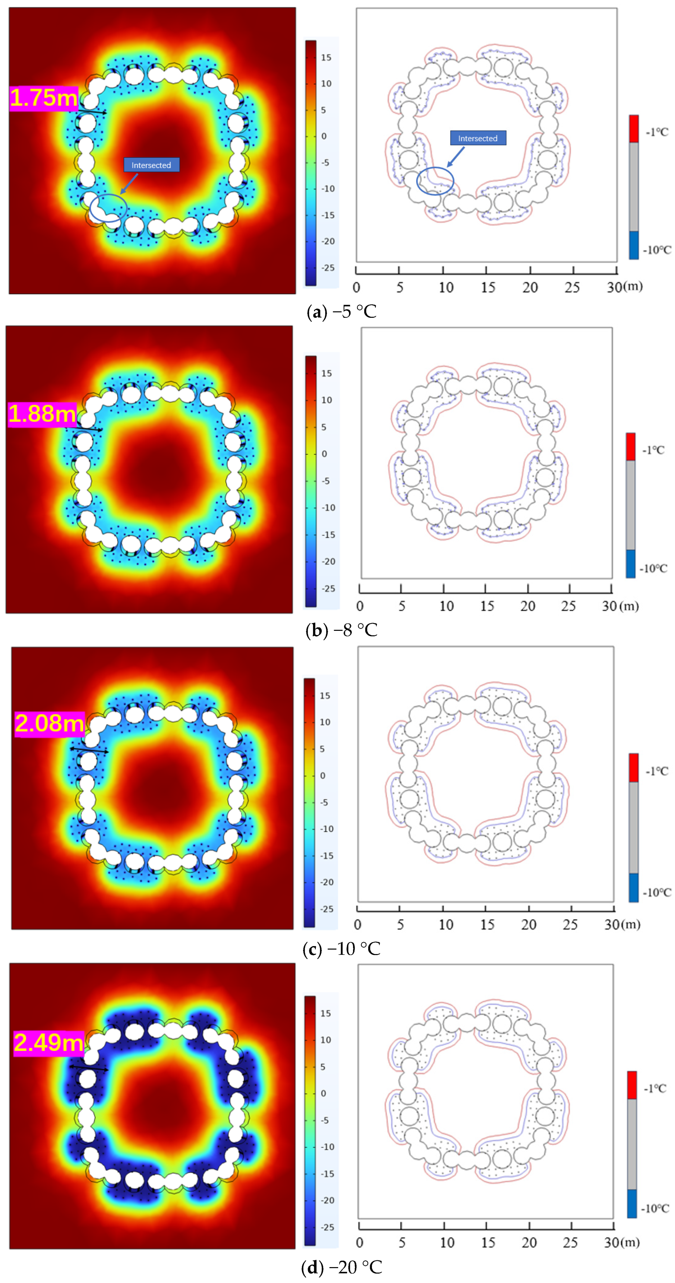
Figure 7 illustrates the distribution of the freezing curtain after 40 days of staged freezing at various temperatures. The thickness of the freezing curtain formed by saline water at −5 °C and −8 °C is 1.75 meters and 1.88 meters, respectively, which do not meet the requirement for a freezing curtain thickness of at least 2 m. In contrast, the thickness of the freezing curtain formed by saline water at −10 °C and −20 °C is 2.08 meters and 2.49 meters, respectively, which satisfy the requirement for a freezing curtain thickness of at least 2 m.

Comparing with Figure 6, the −10 °C isotherm at a saline water temperature of −5 °C begins to show signs of intersection, and the −1 °C isotherm has completed the ring-shaped intersection. At saline water temperatures of −8 °C, −10 °C, and −20 °C, the −1 °C and −10 °C isotherms have completed the ring-shaped intersection.

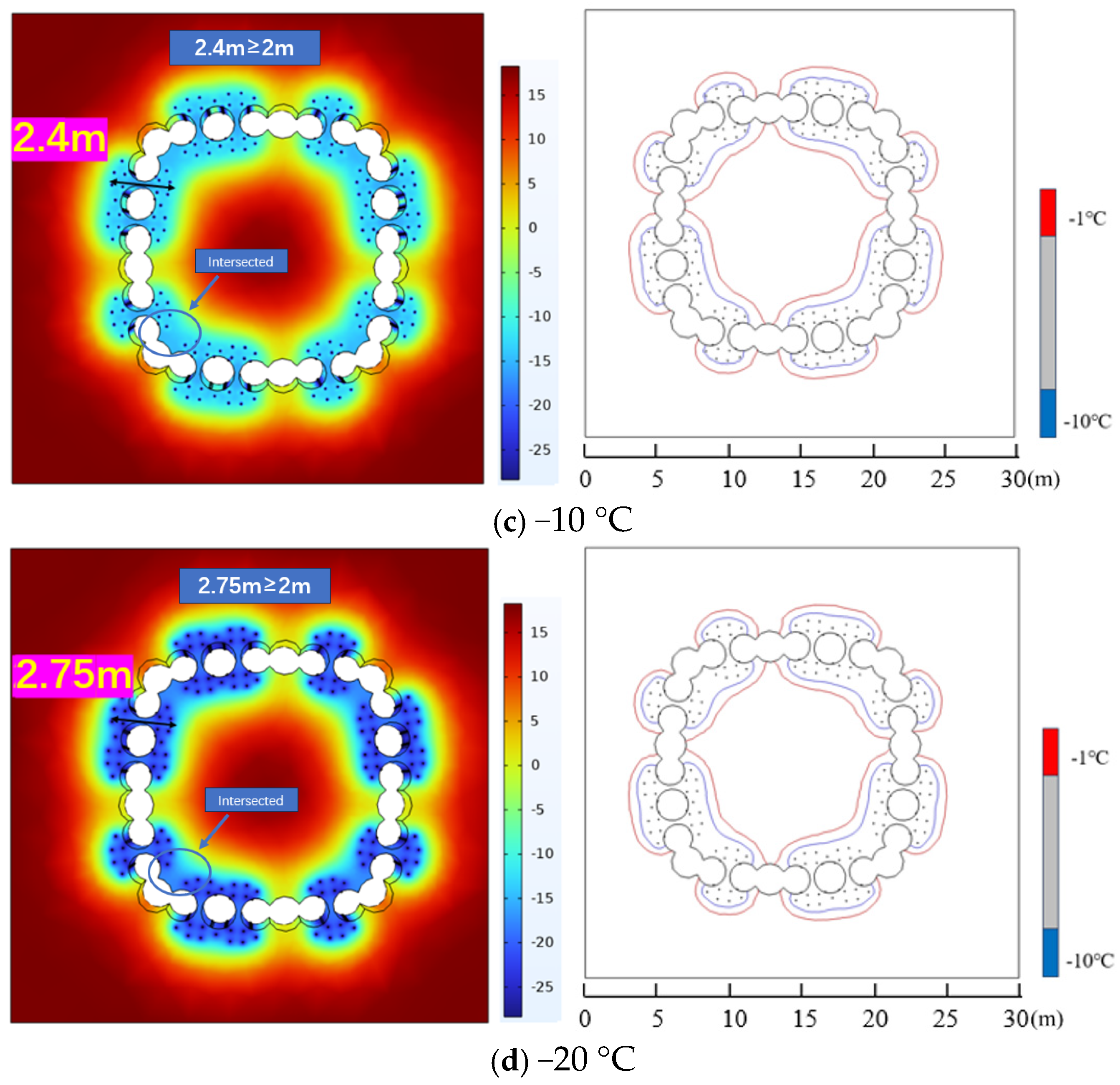
Figure 8 displays the distribution of the freezing curtain at 60 days for each temperature. The final thickness of the freezing curtain formed by saline water at −5 °C is 1.68 m, which is less than the required minimum thickness of 2 m, indicating that the freezing is unsuccessful. In contrast, at saline water temperatures of −8 °C, −10 °C, and −20 °C, the final thicknesses of the freezing curtain are 2.26 meters, 2.4 meters, and 2.75 meters, respectively, all of which meet the requirement for a freezing curtain of at least 2 m. Under no fluid flow conditions, the upstream and downstream freezing curtains are symmetrically distributed. The final study results demonstrate that the saline water cooling plan at −5 °C is insufficient to achieve the desired freezing effect on the soil, while the plans at −8 °C, −10 °C, and −20 °C are effective in meeting the requirements.

Compared to Figure 6 and Figure 7, at a saline water temperature of −5 °C, the −10 °C isotherm has not completed the ring-shaped intersection by the end. In contrast, at saline water temperatures of −8 °C, −10 °C, and −20 °C, both the −1 °C and −10 °C isotherms have successfully completed the ring-shaped intersection. The isotherm results indicate that at a saline water temperature of −5 °C, the intersection is incomplete, leading to unsuccessful freezing. For the other temperatures, the intersection is complete, and the freezing process has been successful.

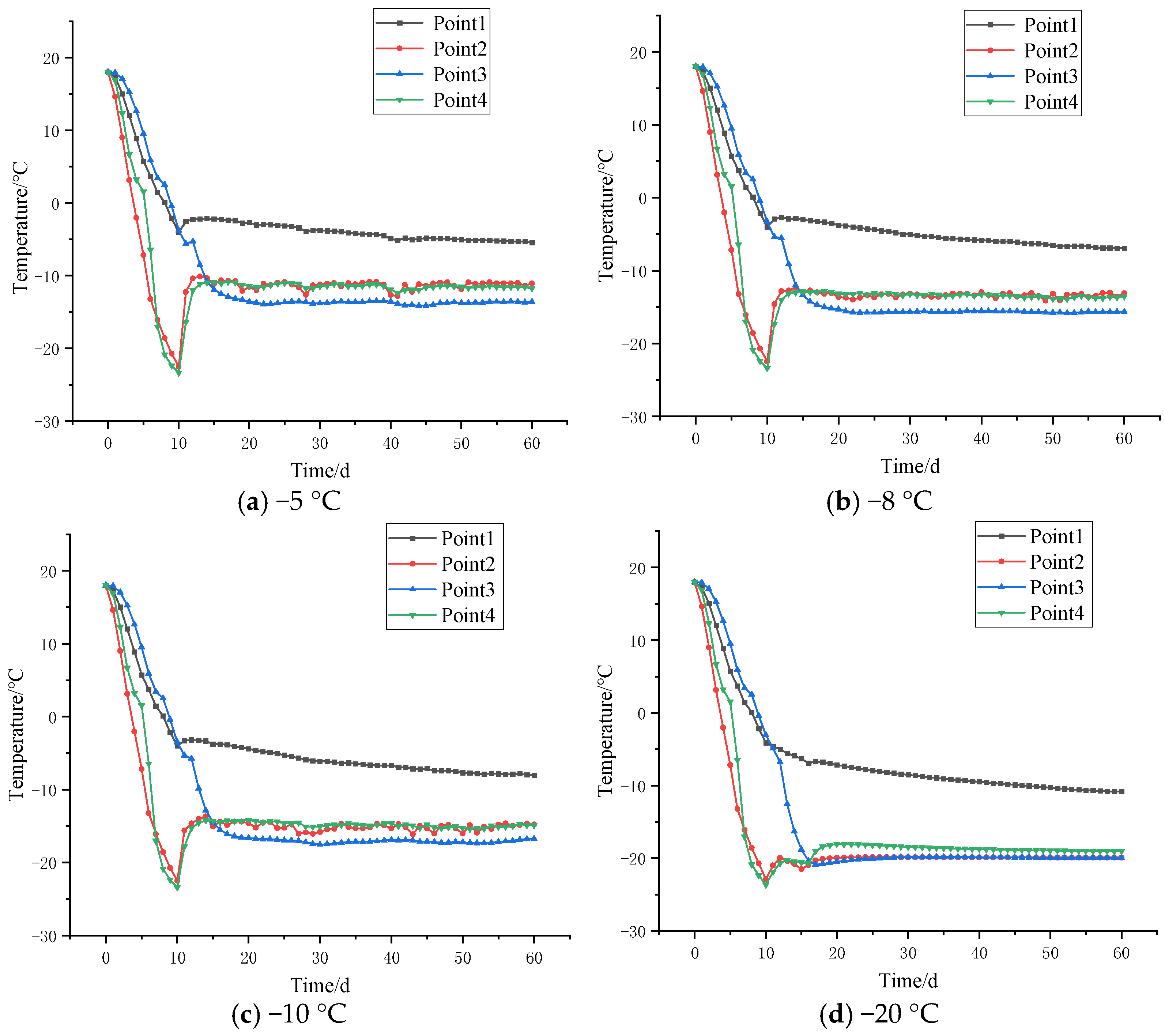
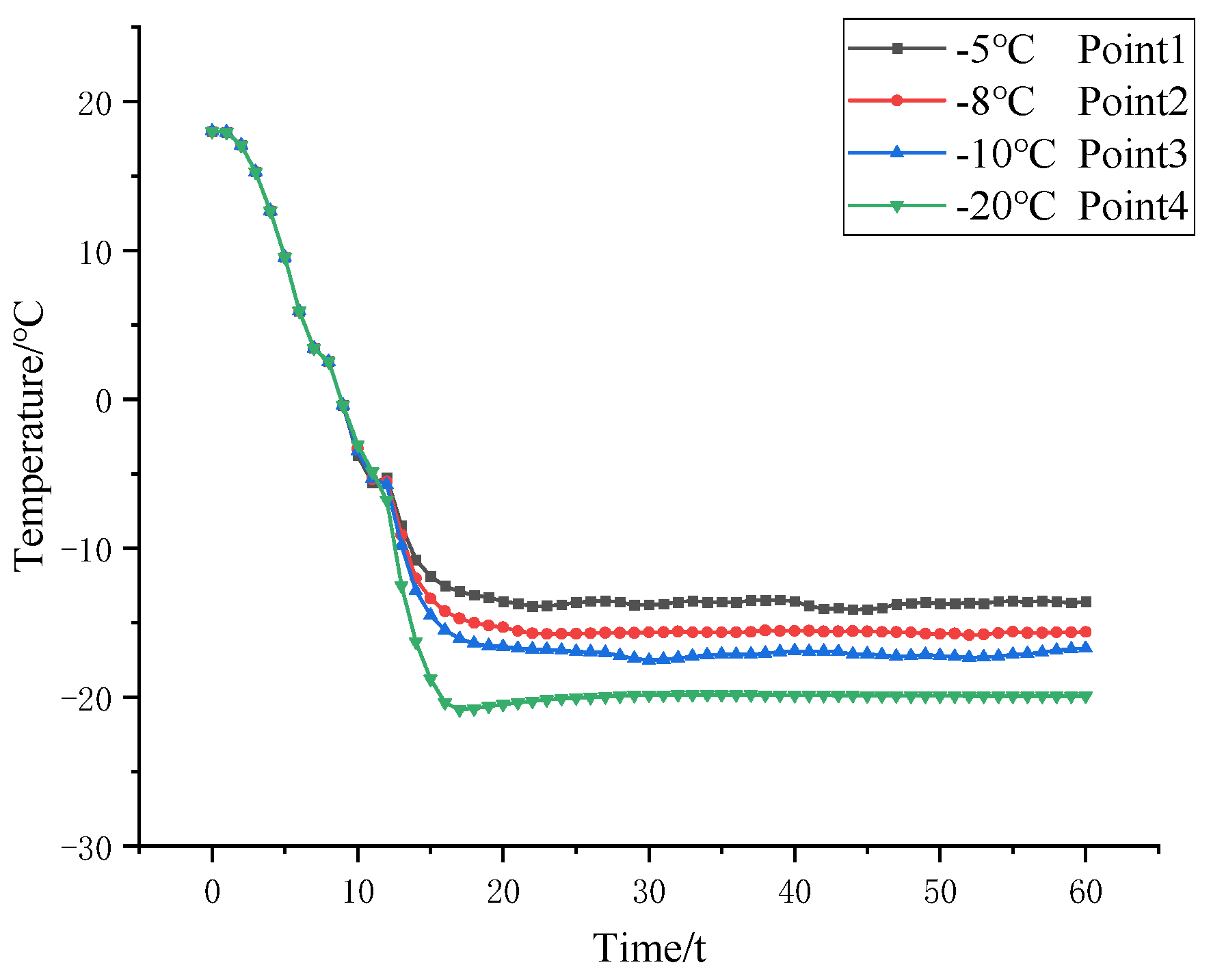
5.2. Observation Point Analysis

Figure 9 presents the temperature cooling curves for four observation points along path 1 under different saline water cooling plans. As shown in the figure, points 2 and 4 are surrounded by freeze protection pipes that are more evenly distributed, resulting in similar temperature change curves. Point 1, being the farthest from the freeze protection pipes, exhibits the highest temperature. Point 3, surrounded by the most freeze protection pipes, achieves the lowest final temperature. Prior to day 10, when the staged freezing plan commenced, the temperature change curves were identical for all plans.

At a saline water temperature of −5 °C, on day 10, the temperatures at points 2 and 4 are −23.3 °C and −22.5 °C, respectively, while at points 1 and 3, they are −3.8 °C and −4 °C, respectively. At this stage, the soil temperature at all four observation points is below 0 °C, indicating the onset of freezing. However, on day 10, when the staged freezing plan began, the temperatures at the four points started to rise. The average temperature at point 3 is approximately −13.5 °C, while the average temperatures at points 2 and 4 are around −11 °C. The temperature at point 1 is approximately −5.1 °C. The final average temperatures of the soil at points 2 and 4 are too high, leading to low freezing efficiency and failing to meet the temperature requirements necessary for the formation of the freezing curtain.

At a saline water temperature of −8 °C, the final average temperatures at points 2 and 4 are approximately −13.5 °C, and at points 1 and 3 are −7 °C and −15.6 °C, respectively. The freezing temperature at point 1, which is the farthest from the freeze protection pipes, is higher than −10 °C and does not meet the requirements for the formation of the freezing curtain. The temperatures at the other three points are below −10 °C and meet the requirements for the formation of the freezing curtain. At a saline water temperature of −10 °C, the final average temperatures at points 2 and 4 are approximately −14.8 °C, and at points 1 and 3 are −8.1 °C and −16.7 °C, respectively. The situation is similar to that at a saline water temperature of −8 °C, and the frozen soil curtain can also be formed normally. At a saline water temperature of −20 °C, the temperature rise at day 10 is the least, and the freezing of the soil is the most stable. The final average temperatures at points 2 and 3 are approximately −19.9 °C, and at points 1 and 4 are −10.8 °C and −19 °C, respectively. Since the final temperature at point 1 is also below −10 °C, the observation point that is the farthest from the freeze protection pipes can also freeze stably, and thus the freezing curtain is the thickest. After comparison, it is found that:

• As the temperature of the saline water decreases, the final average temperature of the frozen soil increases, and the thickness of the freezing curtain decreases. To achieve a thicker freezing curtain, the temperature of the saline water should be lowered.
• The staged freezing plan at a saline water temperature of −5 °C cannot meet the minimum thickness of the freezing curtain, and the freezing fails. Considering the need to save resources, the saline water cooling plan at a temperature of −8 °C is most suitable.

Considering that the thickness of the frozen soil curtain is related to the minimum temperature of the frozen soil, point 3 is the point with the lowest freezing temperature. The data of point 3 for each plan is shown separately in Figure 10. It can be seen from the figure that at day 10, when the staged freezing plan began, the temperature curve of the saline water at −20 °C dropped the fastest, followed by −10 °C, −8 °C, and −5 °C. The final average temperature of the saline water at −20 °C is the lowest, followed by −10 °C, −8 °C, and −5 °C. As the temperature of the saltwater decreases, the rate of temperature decrease in the permafrost increases, resulting in a lower final average temperature and a thicker layer of permafrost.

6. Analysis of Porewater Flow Impacts

The cold in the soil will be displaced by seepage, and in extreme high-permeability conditions, this may lead to insufficient thickness of the freezing wall. Based on the above information, it can be inferred that under no flow conditions, freezing at a saltwater temperature of −8 °C can achieve stable freezing. However, in actual underground engineering, various factors such as groundwater exist. Considering that the flow effect can influence the formation of the frozen curtain, the water head difference above and below the model is set to ∆H = 10 and 20 m, respectively. The corresponding average Darcy flow velocity is calculated to be V = 2.87 m/d and 5.75 m/d, respectively, using Formulas (3) and (4). The changes in isotherms during the freezing plan at a saltwater temperature of −8 °C are studied under low and high flow conditions, respectively.

6.1. Low Flow Conditions

As shown in Figure 11, under an average Darcy flow velocity of V = 2.87 m/d, after 20 days of staged freezing, the thickness of the frozen curtain at the upstream is 1.61 m, and at the downstream, it is 1.65 m. The −1 °C isotherm has completed its loop, and the −10 °C isotherm has started its loop. After 40 days, the thickness of the frozen curtain at the upstream and downstream is 1.86 m and 1.89 m, respectively. The −1 °C and −10 °C strong freezing zones have completed their loops, and the isotherms are displaced from upstream to downstream. After 60 days, the thickness of the frozen curtain at the upstream and downstream reaches 2.24 m and 2.29 m, respectively, satisfying the requirement that the thickness of the frozen curtain ≥ 2 m. The isotherms expand further, and the displacement of the −1 °C isotherm is evident. Under low flow conditions, adjusting the temperature of the saltwater for staged freezing can meet the freezing requirements. Compared to the condition without flow, the thickness of the frozen curtain at the upstream and downstream does not show symmetrical distribution. The thickness of the frozen curtain at the upstream side slightly decreases, while the thickness at the downstream side slightly increases. The cold energy in the soil is transported from the upstream to the downstream through flow, weakening the freezing effect at the upstream and enhancing it at the downstream.

6.2. High Flow Conditions

The freezing changes under high flow conditions with an average Darcy flow velocity of V = 5.75 m/d are shown in Figure 12. After 20 days, the thickness of the frozen curtain at the upstream and downstream is 1.55 m and 1.69 m, respectively. The −10 °C isotherm has completed its loop and begins to shift downstream. The −1 °C isotherm has not completed its loop at the upstream but has at the downstream. After 40 days, the thickness of the frozen curtain at the upstream and downstream is 1.77 m and 1.94 m, respectively. The −10 °C and −1 °C isotherms have completed their loops, and the −10 °C isotherm shows a significant shift downstream. After 60 days, the thickness of the frozen curtain at the upstream and downstream is 2.12 m and 2.36 m, respectively, satisfying the requirement that the thickness of the frozen curtain ≥ 2 m and freezing is successful. The isotherms shift from upstream to downstream and further expand outward. Compared to the conditions without flow and low flow, staged freezing under high flow conditions can also achieve the freezing effect. However, under high flow velocity, the final thickness of the frozen curtain at the upstream is only 2.12 m, which is close to the minimum requirement of 2 m. When the flow conditions are too large, there may be a risk that the frozen curtain thickness at the upstream is less than or equal to 2 m, failing to meet the freezing conditions.

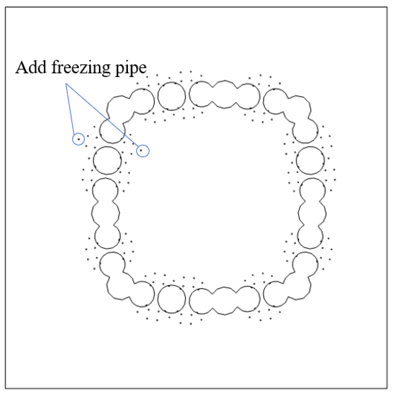
6.3. Addition of Freezing Pipes

The flow effect under high flow conditions can affect the formation of the frozen curtain. Therefore, the method of adding freezing pipes is proposed to address this issue. Two freezing pipes are added at the upstream where the pipe curtain connection is weak to study the effect of this method on the freezing effect of the soil. The addition of freezing pipes is shown in Figure 13.

As shown in Figure 14, under high flow conditions, after 60 days of freezing, the addition of two freezing pipes at the weak part of the upstream frozen curtain has increased the thickness of the frozen curtain to 3.12 m, which is nearly 1 m thicker than the 2.12 m observed in Figure 12. The thickness of the frozen curtain has significantly increased, and the −1 °C and −10 °C isotherms have shown a substantial outward expansion. Overall, the addition of freezing pipes can greatly enhance the freezing efficiency of the soil. In situations where flow conditions are too strong, the thickness of the frozen curtain can be effectively increased by adding more freezing pipes.

7. Conclusions

This paper uses the finite element software COMSOL to simulate the temperature field of the pipe curtain freezing under different plans for the cooling of saltwater. The development laws of the staged freezing are studied. The main conclusions are as follows:

(1)

Staged freezing at a saltwater temperature of −5 °C cannot meet the minimum requirement for the thickness of the frozen curtain. Freezing fails. At a saltwater temperature of −8 °C, the requirement for thickness can be met. The best plan for resource savings is to cool the saltwater to a temperature of −8 °C.

(2)

A higher temperature in the plan for cooling the saltwater inhibits the looping of the isotherms. At a saltwater temperature of −5 °C, the −1 °C isotherm cannot complete its loop. At a saltwater temperature of −8 °C, the −1 °C isotherm can complete its loop. The lower the temperature, the faster the looping speed and the faster the diffusion rate of the isotherms.

(3)

Adjusting the temperature of the saltwater cooling plan for staged freezing to a lower temperature results in a thicker frozen curtain. In practical engineering, staged freezing can be used to meet the freezing requirements by adjusting the saltwater cooling plan, thereby achieving the goal of saving resources.

(4)

The internal flow in the soil has an impact on the formation of the frozen curtain. Without flow, the thickness of the frozen curtain is symmetrically distributed on both sides. Under low flow conditions, the frozen curtain shifts in the direction of the flow, and under high flow conditions, the flow transports a large amount of cold energy from the upstream to the downstream, causing a significant shift in the frozen curtain.

(5)

When the flow velocity is too large, one side may achieve the freezing effect while the other side fails. By reducing the water head difference in the freezing area or adding freezing pipes, the impact of flow on the frozen curtain can be reduced, and the freezing effect can be improved.

This study concludes that the best freezing brine temperature is −8 °C. According to the actual engineering needs, the brine temperature can be appropriately reduced to meet the thickness requirements of the freezing curtain. Seepage will affect the formation of the freezing curtain. Under the condition of excessive seepage speed, it may lead to freezing failure. In the future practical engineering, the brine temperature should be adjusted appropriately under the premise of ensuring the safety and stability of the project.

References

- Song, Z.; Yang, Z.; Huo, R.; Zhang, Y. Inversion Analysis Method for Tunnel and Underground Space Engineering: A Short Review. Appl. Sci. 2023, 13, 5454. [Google Scholar] [CrossRef]
- Li, R.; Zhang, D.; Wu, P.; Fang, Q.; Li, A.; Cao, L. Combined Application of Pipe Roof Pre-SUPPORT and Curtain Grouting Pre-Reinforcement in Closely Spaced Large Span Triple Tunnels. Appl. Sci. 2020, 10, 3186. [Google Scholar] [CrossRef]
- Ren, J.; Wang, Y.; Wang, T.; Hu, J.; Wei, K.; Guo, Y. Numerical Analysis of the Effect of Groundwater Seepage on the Active Freezing and Forced Thawing Temperature Fields of a New Tube–Screen Freezing Method. Sustainability 2023, 15, 9367. [Google Scholar] [CrossRef]
- Hong, Z.; Zhang, J.; Han, L.; Wu, Y. Numerical Study on Water Sealing Effect of Freeze-Sealing Pipe-Roof Method Applied in Underwater Shallow-Buried Tunnel. Front. Phys. 2022, 9, 794374. [Google Scholar] [CrossRef]
- Hu, X.; Wu, Y.; Li, X. A Field Study on the Freezing Characteristics of Freeze-Sealing Pipe Roof Used in Ultra-Shallow Buried Tunnel. Appl. Sci. 2019, 9, 1532. [Google Scholar] [CrossRef]
- Liu, J.; Ma, B.; Cheng, Y. Design of the Gongbei tunnel using a very large cross-section pipe-roof and soil freezing method. Tunn. Undergr. Space Technol. 2018, 72, 28–40. [Google Scholar] [CrossRef]
- Cai, H.; Hong, R.; Xu, L.; Wang, C.; Rong, C. Frost heave and thawing settlement of the ground after using a freeze-sealing pipe-roof method in the construction of the Gongbei Tunnel. Tunn. Undergr. Space Technol. 2022, 125, 104503. [Google Scholar] [CrossRef]
- Zhang, S.; Yue, Z.; Lu, X.; Zhang, Q.; Sun, T.; Qi, Y. Model test and numerical simulation of foundation pit constructions using the combined artificial ground freezing method. Cold Reg. Sci. Technol. 2023, 205, 103700. [Google Scholar] [CrossRef]
- Zhang, S.; Yue, Z.; Sun, T.; Zhang, J.; Huang, B. Analytical determination of the soil temperature distribution and freezing front position for linear arrangement of freezing pipes using the undetermined coefficient method. Cold Reg. Sci. Technol. 2021, 185, 103253. [Google Scholar] [CrossRef]
- Duan, Y.; Rong, C.; Long, W. Numerical Simulation Study on Frost Heave during the Freezing Phase of Shallow-Buried and Undercut Tunnel Using the Freeze-Sealing Pipe Roof Method. Appl. Sci. 2023, 13, 10344. [Google Scholar] [CrossRef]
- Hu, X.; Deng, S.; Ren, H. In Situ Test Study on Freezing Scheme of Freeze-Sealing Pipe Roof Applied to the Gongbei Tunnel in the Hong Kong-Zhuhai-Macau Bridge. Appl. Sci. 2017, 7, 27. [Google Scholar] [CrossRef]
- Qi, Y.; Zhang, J.; Yang, H.; Song, Y. Application of Artificial Ground Freezing Technology in Modern Urban Underground Engineering. Adv. Mater. Sci. Eng. 2020, 2020, 1619721. [Google Scholar] [CrossRef]
- Ou, Y.; Wang, L.; Bian, H.; Chen, H.; Yu, S.; Chen, T.; Satyanaga, A.; Zhai, Q. Numerical Analyses of the Effect of the Freezing Wall on Ground Movement in the Artificial Ground Freezing Method. Appl. Sci. 2024, 14, 4220. [Google Scholar] [CrossRef]
- Hu, J.; Liu, Y.; Wei, H.; Yao, K.; Wang, W. Finite-Element Analysis of Heat Transfer of Horizontal Ground-Freezing Method in Shield-Driven Tunneling. Int. J. Géoméch. 2017, 17, 04017080. [Google Scholar] [CrossRef]
- Huang, S.; Guo, Y.; Liu, Y.; Ke, L.; Liu, G.; Chen, C. Study on the influence of water flow on temperature around freeze pipes and its distribution optimization during artificial ground freezing. Appl. Therm. Eng. 2018, 135, 435–445. [Google Scholar] [CrossRef]
- Zhou, J.; Hu, J.; Liu, B. Numerical simulation analysis of hydro-thermal coupling temperature field of subsea tunnel freezing method. J. For. Proj. 2024, 40, 221–234. [Google Scholar]
- Li, Z.; Chen, J.; Sugimoto, M.; Ge, H. Numerical simulation model of artificial ground freezing for tunneling under seepage flow conditions. Tunn. Undergr. Space Technol. 2019, 92, 103035. [Google Scholar] [CrossRef]
- Li, M.; Ma, Q.; Luo, X.; Jiang, H.; Li, Y. The coupled moisture-heat process of a water-conveyance tunnel constructed by artificial ground freezing method. Cold Reg. Sci. Technol. 2020, 182, 103197. [Google Scholar] [CrossRef]
- Duan, Y.; Rong, C.; Cheng, H.; Cai, H.; Wang, Z.; Yao, Z. Experimental and Numerical Investigation on Improved Design for Profiled Freezing-tube of FSPR. Processes 2020, 8, 992. [Google Scholar] [CrossRef]