Understanding Congestion Risk and Emissions of Various Travel Behavior Patterns Based on License Plate Recognition Data

Abstract

Understanding vehicle travel behavior patterns is crucial for effectively managing urban traffic congestion and mitigating the associated risks and excessive emissions. Existing research predominantly focuses on commuting patterns, with limited attention given to the spatiotemporal characteristics of other travel behaviors, and sparse investigation into the congestion risks and emissions associated with these patterns. To address this gap, the present study examines various travel behavior patterns and their associated congestion risks and emissions, using one week of License Plate Recognition (LPR) data from the megacity expressway network. First, we classify vehicles into different travel modes based on spatiotemporal features extracted from the LPR data and propose a scalable mode recognition method suitable for large-scale applications. We then assess the congestion risks associated with each mode and estimate the excessive emissions resulting from congestion. The findings reveal notable differences in congestion risks among travel modes, with a bimodal distribution influenced by the temporal rhythm of traffic flow. Furthermore, although commercial vehicles constitute only one-third of the total vehicle population, the excessive emissions attributed to congestion from commercial vehicles are comparable to those from privately owned vehicles. This suggests that focusing exclusively on commuting patterns may underestimate both the congestion risks and excessive emissions. The results of this study not only deepen our understanding of the relationship between individual travel behavior and traffic congestion but also support the optimization of personal travel time and health management, providing a foundation for the development of personalized and proactive traffic demand management strategies.

1. Introduction

Traffic congestion has long been a global challenge, leading to significant time losses and economic costs [1,2]. Moreover, excessive carbon emissions from congested traffic severely degrade the ecological environment, posing considerable risks to public health, both physical and mental [3,4]. These issues hinder the sustainable development of cities. In an effort to alleviate congestion, urban managers have sought to promote changes in travel behavior [5].

On the supply side, the rapid growth of urban populations and the increasing use of private vehicles have placed immense pressure on surface transportation systems, making them inadequate for meeting urban travel demands. In response, the concept of Urban Air Mobility (UAM) has emerged. In 2020, UAM made a significant technological breakthrough with the introduction of Vertical Take-Off and Landing (VTOL) technology, which allows for the operation of specific flight routes. This advancement opens the possibility for UAM to provide point-to-point services. Data from Milan Airport (Italy) show that, at least in the initial phase, high-income individuals traveling for business purposes are most likely to use UAM services [6]. In contrast, highly educated individuals and those whose travel expenses are reimbursed are less inclined to choose UAM for airport access, preferring traditional ground taxis [7]. Meanwhile, a survey conducted in Tehran, the capital of a developing country, suggests that the widespread adoption of UAM remains unfeasible at this stage [8]. However, it is still seen as a potentially viable solution to address persistent congestion issues in metropolitan areas of the Southern Hemisphere. Although UAM is regarded as a method to enhance urban traffic efficiency, reduce ground congestion, and promote sustainable urban growth [9], a significant transition period from ground transportation to UAM is expected, owing to challenges related to battery performance, economic feasibility, safety, and regulation [8,10].

At this juncture, efforts to control congestion and excessive emissions are primarily focused on managing demand. Key regulatory strategies include congestion pricing, license plate restrictions, tradable road rights, and travel demand management. Cities such as Singapore (1975), London (2003), Stockholm (2006), Milan (2008), Gothenburg (2013), Durham (2002), and Valletta (2007) have implemented congestion pricing schemes [11]. However, such strategies, which impose penalties to alter travel behavior, have not been widely accepted due to public opposition, concerns about fairness, and numerous unsuccessful proposals. The most significant challenge remains their limited effectiveness [12]. In addition, scholars have found that developing new energy transportation, promoting green and shared mobility, and implementing dynamic spatiotemporal travel guidance can help alleviate traffic congestion and excessive emissions [13].

The success of these regulatory strategies largely depends on understanding the behavior patterns of individual travelers [14]. Policymakers, for instance, must exercise caution when determining who should bear the cost of congestion charges. Ineffective pricing schemes may impose unnecessary or even harmful burdens on commuters. Additionally, in the realm of travel demand management, Ref. [15] introduced a new route recommendation model that accounts for drivers’ route preferences. However, this model was based on a small-scale survey, limiting its applicability to the entire vehicle population and its suitability for large-scale networks. Similarly, Ref. [16] proposed a route planning method that incorporates predictive uncertainties but focuses exclusively on minimizing travel time, neglecting users’ route preferences. Ultimately, the effectiveness of regulatory strategies hinges on a comprehensive understanding of travelers’ behaviors and the congestion risks they may encounter. Therefore, identifying and understanding travel behavior patterns as well as the congestion risks associated with each pattern are crucial for formulating effective management policies.

Research on travel behavior has traditionally relied on data-driven methods [17,18]. With advancements in information technology, a growing variety of data sources has been incorporated into such studies [19], including License Plate Recognition (LPR) data, mobile signaling data, questionnaire/telephone survey data, and bus card data. In the early stages, travel behavior research primarily utilized travel survey data collected through paper questionnaires, telephone interviews, and online surveys. Using these data, researchers explored various aspects, such as commuters’ travel time preferences [20], travel mode selection [21], and more complex patterns of travel behavior [22]. However, the high cost of collecting survey data limits both sample size and frequency [23], making traditional surveys inadequate for comprehensive studies of travel behavior patterns. Consequently, some researchers have turned to mobile signaling data, which have been used to investigate travel patterns and population distribution [24], infer individual attributes and activity types [25], analyze personal mobility trajectories [26], and mine travel purposes [27]. Despite these applications, mobile phone data pose challenges in accurately inferring individual travel behavior patterns, as they cannot differentiate between transportation modes such as subway, private car, taxi, or bicycle. Similarly, data from bus card transactions fail to provide a holistic representation of overall travel patterns [28].

LPR data offers more comprehensive coverage, enabling the collection of information from all vehicles on the road network and providing detailed insights into vehicle travel time and spatial activities. As a result, multi-day vehicle trajectory data derived from LPR presents new opportunities for in-depth studies on travel behavior patterns. For example, Ref. [29] explored the impact of two different vehicle restriction policies on traffic conditions, finding that these restrictions led to more “illegal” travel and increased travel intensity. Ref. [30] examined the effects of vehicle traffic restrictions on the behavior of non-Shanghai licensed vehicles, analyzing their travel patterns. Ref. [31] proposed a method to assess travel behavior regularity based on the order of travel or activity organization, categorizing travel behavior patterns into conventional and unconventional types. Sun et al. [32] used LPR data to identify both regular and abnormal patterns in individual travel behavior. However, the distinction between conventional and unconventional patterns is insufficient to support sophisticated demand management strategies. Ref. [33] developed multiple indicators to represent commuting patterns by utilizing vehicle travel OD information, extracting commuting rules through clustering and decision tree algorithms. Ref. [34] also leveraged LPR data from Cambridge, UK, to study the non-commuting travel demand of commuters. Ref. [5] proposed a systematic method for identifying travel behaviors and purposes based on weekly trajectory data from 6600 trams in Shanghai. Using a Gaussian mixture model, they categorized vehicle travel behavior into four groups, including commuting. However, the algorithm’s complexity limits its application to large-scale road networks. The use of LPR data effectively addresses issues such as small sample sizes, low data quality, and difficulties in acquisition, which are inherent in traditional survey methods. Research on travel behavior patterns based on LPR data has gradually become a key component of the human mobility theory framework. However, the full potential of LPR data remains largely untapped. Currently, most studies focus on analyzing traffic flow and commuting patterns between origin and destination points (OD points), often limiting their exploration to single-mode travel patterns. This narrow approach overlooks critical factors such as route preferences, time preferences, and travel distances. In reality, travelers’ route choices are not only influenced by traffic flow and congestion but are also closely linked to individual travel habits and time schedules. These factors significantly affect travel behavior patterns and must be considered in future research. Therefore, studies on travel behavior patterns based on LPR data should place greater emphasis on exploring these key characteristics. Moreover, existing studies largely rely on empirically derived parameters and indicators [35,36]. Many studies propose hypotheses based on theoretical deductions derived from observations of limited data; however, the applicability and generality of these hypotheses still require validation through data mining and model testing. Therefore, future research should focus on optimizing the design of characteristic indicators for travel behavior patterns, utilizing data-driven approaches to analyze the multidimensional aspects of travel routes, time, and distance. This would provide a more accurate foundation for the development of traffic management policies.

Traffic congestion risk can be defined as the potential threat posed by excessive or unevenly distributed traffic flow, leading to delays in road network mobility and resulting in increased vehicle delays, traffic accidents, environmental pollution, and other negative consequences. Current research on traffic congestion risk mainly focuses on commuting patterns, with relatively little attention paid to other travel behavior patterns. For instance, Ref. [37] examined how traffic congestion affects individual commuting satisfaction, highlighting the relationship between commuting duration and personal health. Similarly, Ref. [38] explored the perceived differences between individuals using different modes of transportation during periods of congestion. Given that commuting is often associated with higher congestion risks, Ref. [39] proposed strategies, such as staggered work hours, to alleviate congestion during peak periods. However, the feasibility and sustainability of these strategies remain debated, and their effectiveness may vary across different travel modes. In reality, road networks accommodate various travel modes [40], and focusing solely on commuting patterns may underestimate the overall congestion risk. Therefore, strategies to mitigate traffic congestion should consider a broader range of travel behaviors, not just commuting patterns, to more comprehensively assess and address congestion risks.

Additionally, existing research has paid relatively little attention to the relationship between traffic congestion and environmental pollution, particularly concerning excessive emissions. While traffic congestion is widely recognized as a significant contributor to increased emissions, many studies focus primarily on the impact of congestion on traffic flow, with limited attention given to the emission problems it causes. The low speeds or stagnation of vehicles in congestion lead to increased fuel consumption and greater exhaust emissions, exacerbating air pollution and contributing to greenhouse gas emissions. Therefore, the environmental and health risks posed by congestion are urgent issues that require attention. Future research should systematically explore the relationship between traffic congestion and excessive emissions, integrating these findings into traffic management and policy frameworks to promote sustainable transportation development and environmental protection.

Based on the background described above, this paper first preprocesses and generates trajectories from one week of LPR data collected on the expressway network of a city in China. It then constructs multiple novel spatiotemporal features and applies three different clustering methods to classify vehicle categories. Subsequently, a pattern recognition model is developed using LightGBM (Light Gradient Boosting Machine). The congestion risks and excess emissions associated with each pattern are analyzed, followed by recommendations for congestion management strategies. The contributions of this paper are as follows:

• A novel method for dividing travel behavior patterns based on a unique set of spatiotemporal feature indicators is proposed. This method uses clustering to identify homogeneous clusters from data features, overcoming the subjectivity and limitations of traditional threshold-based approaches.
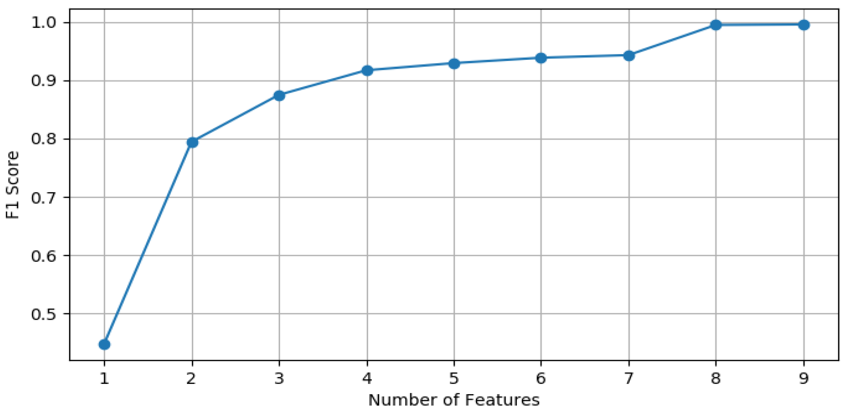
• A pattern recognition method suitable for large-scale applications is presented, demonstrating strong recognition performance with only three feature values.
• The congestion risks and excess emissions of various travel patterns are analyzed based on real-world LPR data. The findings offer important insights for individual travel time planning and health management, and provide support for the development of personalized, proactive traffic demand management measures.

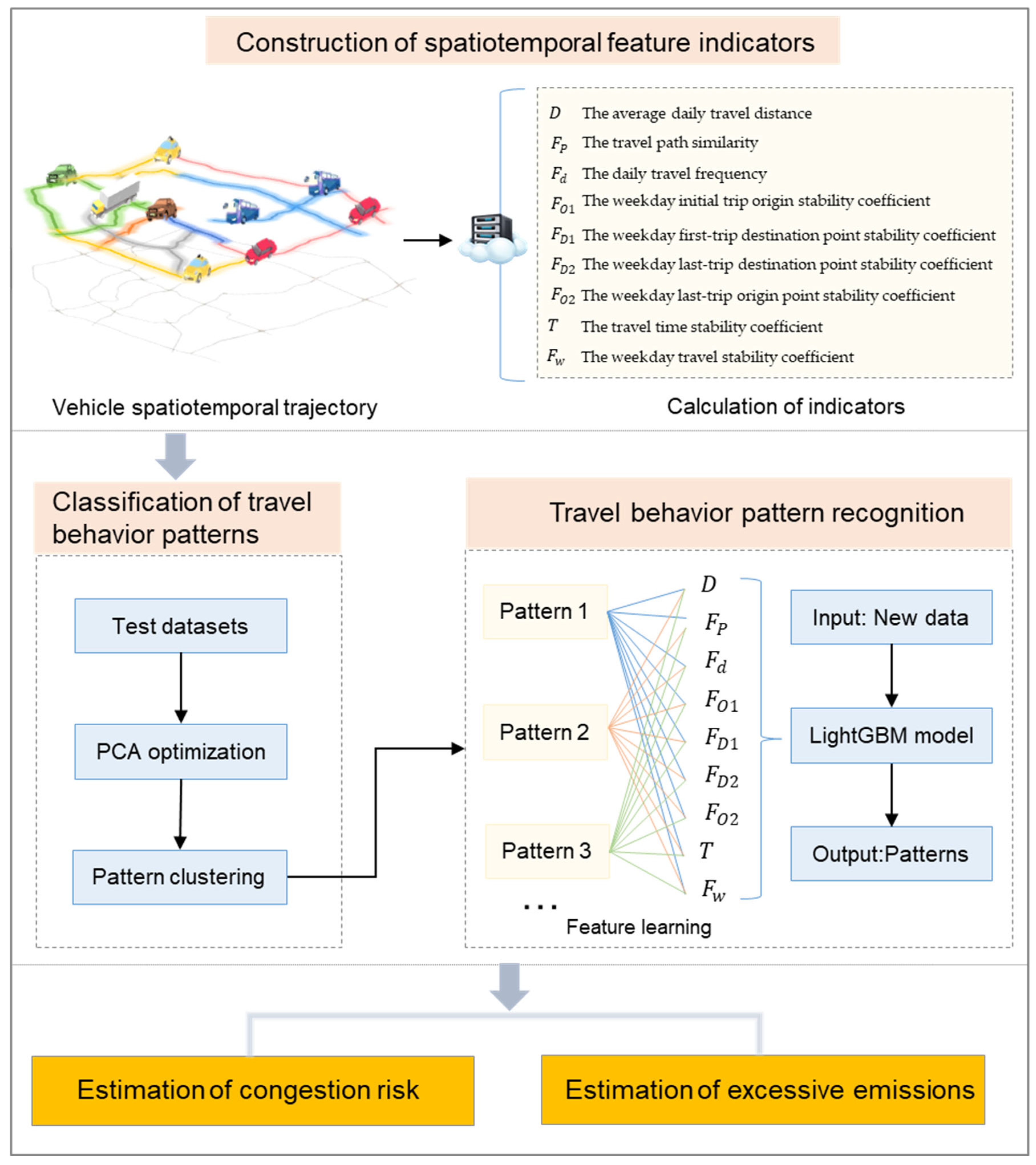
The remaining sections of this paper are organized as follows: Section 2 introduces the data sources, pattern recognition methods, and the estimation methods for congestion risks and excess emissions. Section 3 presents the experimental results based on real-world LPR data. Section 4 discusses the congestion risks of each pattern and proposes strategies for congestion mitigation. Finally, Section 5 concludes the study.

2. Methodology

The congestion risk estimation method for various travel behavior patterns proposed in this paper is illustrated in Figure 1. The study is structured into three key components: (1) the construction of spatiotemporal characteristic indices for travel behavior, (2) the classification and recognition of travel behavior patterns, and (3) the estimation of congestion risk. Each of these components is described in detail in the following sections.

2.1. Identification of Travel Behavior Patterns

2.1.1. Construction of Spatiotemporal Feature Indicators

Daily travel patterns are influenced by activity demands, with each trip linked to specific spatiotemporal activities at the destination, which in turn shape the characteristics of the trip and the associated travel behavior patterns. Understanding these patterns is essential for effective traffic demand management, urban planning, and resource allocation [28]. In this study, nine indicators were developed using LPR data to capture the spatiotemporal features of travel behavior comprehensively.

The weekday travel stability coefficient, $F_w$, is defined as follows:

$$F_w={\displaystyle \frac{n_w}{N}}$$

(1)

where $N$ represents the total number of weekdays surveyed, and $n_w$ denotes the number of days a particular vehicle was detected.

The daily travel frequency, $F_d$, is defined as follows:

$$F_d={\displaystyle \frac{n_d}{N}}$$

(2)

where $n_d$ represents the total number of trips made by a specific vehicle within the statistical scope.

The frequency of visits is a key component in the theoretical framework of human mobility, i.e., the number of times someone travels to a location per unit of time [41]. Building upon this notion, this study extracts the initial and final travel trajectories of individual vehicles on a daily basis using LRP data, characterizing the spatial stability of travel behavior through the access frequency of these start and end points. Assuming that within the study timeframe, the starting points of vehicles’ first and last daily trips are denoted as $O_1$ and $O_2$, respectively, and the corresponding end points as $D_1$ and $D_2$.

The weekday initial trip origin stability coefficient, $F_{O1}$, is defined as follows:

$$F_{O1}={\displaystyle \frac{\mathrm{m}\mathrm{a}\mathrm{x}(f_{O_1},f_{O_2},\dots ,f_{O_n})}{n_w}}$$

(3)

where ${\mathrm{m}\mathrm{a}\mathrm{x}(f}_{On})$ represents the number of times the highest frequency origin point appears for a vehicle’s first trip during weekdays.

The weekday last-trip origin point stability coefficient, $F_{O2}$, is defined as follows:

$$F_{O2}={\displaystyle \frac{\mathrm{m}\mathrm{a}\mathrm{x}(l_{O_1},l_{O_2},\dots ,l_{O_n})}{n_w}}$$

(4)

where ${\mathrm{m}\mathrm{a}\mathrm{x}(l}_{On})$ denotes the number of times the highest frequency origin point appears for a vehicle’s last trip during weekdays.

The weekday first-trip destination stability coefficient, $F_{D1}$, is defined as follows:

$$F_{D1}={\displaystyle \frac{\mathrm{m}\mathrm{a}\mathrm{x}(f_{D_1},f_{D_2},\dots ,f_{D_n})}{n_w}}$$

(5)

where ${\mathrm{m}\mathrm{a}\mathrm{x}(f}_{Dn})$ represents the number of times the highest frequency destination point appears for a vehicle’s first trip during weekdays.

The weekday last-trip destination stability coefficient, $F_{D1}$, is defined as follows:

$$F_{D1}={\displaystyle \frac{\mathrm{m}\mathrm{a}\mathrm{x}(l_{D_1},l_{D_2},\dots ,l_{D_n})}{n_w}}$$

(6)

where ${\mathrm{m}\mathrm{a}\mathrm{x}(l}_{Dn})$ denotes the number of times the highest frequency destination point appears for a vehicle’s last trip during weekdays.

In addition to the frequency of visits to origin and destination points, path similarity can also characterize the spatial stability of travel behavior. The difference lies in that path similarity focuses on the overall frequency of traversed paths and can also reflect the vehicle’s path preferences. This study calculates path similarity based on the Jaccard coefficient.

The travel path similarity, $F_P$, is defined as follows:

$$F_P={\displaystyle \frac{\left|P_1\cap P_2\cap \dots \cap P_{n_w}\right|}{\left|P_1\right|+\left|P_2\right|+\dots +\left|P_{n_w}\right|-\left|P_1\cap P_1\cap \dots \cap P_{n_w}\right|}}$$

(7)

where $P_{n_w}$ represents the set of road segments for a particular travel path.

Considering the extraction of comprehensive spatiotemporal features from massive LPR data, this study utilizes the average daily travel distance to characterize the spatial features of travel behavior.

The average daily travel distance, $D$, is defined as follows:

$$D={\displaystyle \frac{\sum _{i=1}^{n_d}{D}_i}{100N}}$$

(8)

where $D_i$ represents the distance traveled by a vehicle in a single trip, in kilometers.

Regarding the temporal features of travel behavior, existing studies often use travel periods for characterization. For instance, Ref. [33] identifies commuting patterns based on travel during morning and evening peak periods. However, regardless of commuting or other travel patterns, they may not necessarily be concentrated during these peak periods. Therefore, considering that travel times can be obtained from LPR data, this study utilizes the standard deviation of the time of the first trip on workdays to characterize the temporal features of travel behavior while also reflecting the sensitivity of travelers to time constraints.

The travel time stability coefficient, $T$, is defined as follows:

$$T=\left\{\begin{array}{c}1,\\ 0,\end{array}\right.\begin{array}{c}\sigma \le 30\\ \sigma >30\end{array}, \sigma =\sqrt{{\displaystyle \frac{\sum _{i=1}^n{(t_i-\overline{t})}^2}{n}}}$$

(9)

where $t_i$ represents the time of the first trip on a workday for a vehicle, and $\overline{t}$ represents the average time of the first trip on a workday for a vehicle. After statistical analysis, when the standard deviation of the time of the first trip on workdays within the study road network is 30 min, this grouping has the largest proportion. Therefore, $\sigma$ is set to 30.

2.1.2. Classification of Travel Behavior Patterns

Based on the aforementioned spatiotemporal feature indicators, we aim to reduce the dimensionality of each feature variable to eliminate correlations, summarize existing observed variables with fewer latent variables, and improve clustering algorithm efficiency. To address the uneven distribution of feature data, we apply various clustering algorithms for pattern classification and compare their performance to select the optimal algorithm. The process is as follows:

(1) Dimensionality Reduction: Before reducing the dimensionality of each feature, we first conduct KMO and Bartlett’s tests to evaluate the suitability of the data structure for dimensionality reduction. Next, we determine the number of principal components based on the Kaiser criterion, scree plot, and variance explanation criterion [42], and then we perform dimensionality reduction.

(2) Determination of the Optimal Number of Clusters: After dimensionality reduction, we determine the optimal number of clusters to partition travel behavior patterns, typically using the elbow method. The core idea behind the elbow method is as follows: when the number of clusters, $\mathrm{k}$, is smaller than the actual number of clusters, increasing $\mathrm{k}$ significantly enhances intra-cluster cohesion, which leads to a large decrease in the within-cluster sum of squares (Inertia). However, as $\mathrm{k}$ approaches the true number of clusters, further increases in $\mathrm{k}$ result in diminishing returns, and the rate of decrease in Inertia flattens out. This relationship between Inertia and $\mathrm{k}$ forms an elbow shape, where the “elbow point” indicates the optimal number of clusters. The formula for calculating the within-cluster sum of squares is shown below.

$$\mathrm{I}\mathrm{n}\mathrm{e}\mathrm{r}\mathrm{t}\mathrm{i}\mathrm{a}={\sum }_{p\in C_i}{\left|p-m_i\right|}^2$$

(10)

where $C_i$ represents the $i$ cluster, $p$ is a sample point in cluster $C_i$, and $m_i$ is the centroid of the cluster.

(3) Clustering. After determining the optimal number of clusters, we apply three clustering algorithms—K-means, Agglomerative Clustering, and DBSCAN (Density-Based Spatial Clustering of Applications with Noise)—to analyze the dataset. The K-means algorithm partitions the data into K clusters, ensuring high similarity among data points within each cluster. Agglomerative Clustering, a distance-based hierarchical method, iteratively merges data points into clusters, minimizing internal distances and maximizing external distances. DBSCAN, a density-based algorithm, forms clusters by identifying regions of high data point density. These three methods are employed to uncover distinct travel behavior patterns across all vehicles. The clustering results are evaluated using the silhouette coefficient, as defined in Equation (11).

$$S={\displaystyle \frac{b-a}{\mathrm{m}\mathrm{a}\mathrm{x}(a,b)}}$$

(11)

Here, $a$represents the average distance between sample $x_i$ and other samples within the same cluster, referred to as cohesion, while $b$ denotes the average distance between $x_i$ and all samples in the nearest cluster, known as separation. The silhouette coefficient ranges from −1 to 1, with values closer to 1 indicating better clustering performance. A value less than zero indicates poor clustering performance, with many points misclassified.

2.1.3. Travel Behavior Pattern Recognition

After partitioning patterns based on historical LPR data, an efficient classifier must be constructed to recognize patterns among a large number of vehicles, including newly added ones. To achieve this, we employ the LightGBM (Light Gradient Boosting Machine) algorithm, which is capable of efficiently processing large datasets. LightGBM is an ensemble method based on gradient boosting, and one of its key innovations is the Gradient-based One-Side Sampling (GOSS) algorithm. GOSS selectively retains instances with larger gradients while randomly sampling instances with smaller gradients. Specifically, the GOSS algorithm first sorts instances by the absolute values of their gradients and selects the top “a” instances. Then, it randomly samples “b” instances from the remaining data. In the process of calculating information gain, the algorithm multiplies the gradients of the sampled instances with smaller gradients by (1−a)/b. This strategy enables the algorithm to focus more on underrepresented instances while maintaining the overall distribution of the original dataset. Let O represent the training dataset at a fixed node of the decision tree. The variance gains of splitting feature $\mathrm{j}$ at point $d$ for this node is defined as follows:

$$V_{\left.j\right|O}(d)={\displaystyle \frac{1}{n_O}}({\displaystyle \frac{{({\sum }_{\left\{x_i\in O:x_{ij}\le d\right\}}{g}_i)}^2}{n_{\left.l\right|O}^j(d)}}+{\displaystyle \frac{{({\sum }_{\left\{x_i\in O:x_{ij}>d\right\}}{g}_i)}^2}{n_{\left.r\right|O}^j(d)}})$$

(12)

where $n_O=\sum I\left[x_i\in O\right]$, $n_{\left.l\right|O}^j\left(d\right)=\sum I\left[x_i\in O:x_i\le d\right]$,$n_{\left.r\right|O}^j(d)=\sum I\left[x_i\in O:x_i>d\right]$.

The formula for calculating the estimated variance gain, ${\tilde{V}}_j\left(d\right)$, of the GOSS algorithm is as follows:

$${\tilde{V}}_j(d)={\displaystyle \frac{1}{n}}({\displaystyle \frac{{({\sum }_{\left\{x_i\in A:x_{ij}\le d\right\}}{g}_i+\frac{1-a}{b}{\sum }_{\left\{x_i\in B:x_{ij}\le d\right\}}{g}_i)}^2}{n_l^j(d)}}+{\displaystyle \frac{{({\sum }_{\left\{x_i\in A:x_{ij}>d\right\}}{g}_i+\frac{1-a}{b}{\sum }_{\left\{x_i\in B:x_{ij}>d\right\}}{g}_i)}^2}{n_r^j(d)}})$$

(13)

$A$represents the subset with larger gradients and $B$ represents the subset with smaller gradients. And ${\displaystyle \frac{1-a}{b}}$ is used to normalize the sum of the gradients over B.

Furthermore, the exclusive feature bundling algorithm can combine many exclusive features into fewer dense features, effectively avoiding unnecessary computation for zero feature values.

In this study, the data samples are divided in a ratio of 0.8:0.2, with 80% of the dataset utilized for training the proposed model and 20% for testing the trained model. Additionally, the F1-score is selected as the measurement method for the classification model in this paper. The F1-score considers both precision and recall, providing a balanced assessment of the model’s accuracy between precision and recall.

2.2. Estimation of Congestion Risk and Excessive Emissions

Based on the aforementioned division of travel patterns, we measure congestion risk by calculating the actual travel time and the ideal travel time for each trip trajectory. The expression for the ideal travel time is given by the following:

$${\displaystyle t_{(1,m)}^i}={\sum }_{j=1}^{n_1}{\displaystyle \frac{L_j}{{\widehat{v}}_j}}$$

(14)

where $t_{(1,m)}^i$ represents the ideal travel time for vehicle $i$ in the $m$th trip, $L_j$ denotes the length of segment$j$,${\widehat{v}}_j$ represents the speed of segment $j$ under free-flow conditions, and$n_1$ denotes the total number of segments for vehicle $i$ in the $j$th trip.

The expression for the actual travel time is given by the following:

$$t_{(2,m)}^i=t_{(end,m)}^i-t_{(start,m)}^i$$

(15)

where $t_{(2,m)}^i$ represents the actual travel time for the vehicle, $i$, in the $m$th trip, $t_{(start,m)}^i$ and $t_{(end,m)}^i$, respectively, represent the start and end times of the trip for the vehicle,$i$, obtained from LPR data.

Therefore, the expression for the congestion exposure time corresponding to the $k$th travel pattern is as follows:

$$T_k={\displaystyle \frac{\sum _1^{n_2}\sum _1^m{(t}_{(2,m)}^i-{rt}_{\left(1,m\right)}^i)}{m{n}_2}}$$

(16)

where $T$ represents the congestion exposure time for a single trip of vehicle data corresponding to the $k$th travel pattern, $r$ represents the preset congestion coefficient [43], taken as 1.5 in this paper, and $n_2$represents the total number of vehicles for the $k$th travel pattern.

In this study, we further estimated the excess CO emissions generated by each vehicle category due to congestion using the Emissions Model for Beijing Vehicles (EMBEV) [44]. We chose to use this model because it has been proven to be more suitable for estimating road emissions in China’s megacities [44,45,46]. The excess emissions, $E_{ex(m)}^i$, generated by the vehicle, $i$, in the $m$th trip due to congestion are as follows:

$$E_{ex(m)}^i=({\sum }_{j=1}^{n_1}EF({\widehat{v}}_j)L_j-{\sum }_{j=1}^{n_1}EF({\displaystyle \frac{L_j}{t_{(end,j)}^i-t_{(start,j)}^i}})L_j)/{\sum }_{j=1}^{n_1}EF({\widehat{v}}_j)L_j$$

(17)

Therefore, the expression for excessive emissions corresponding to the $k$th travel pattern is:

$$E_k={\sum }_1^{n_2}{\sum }_1^m{E}_{ex(m)}^i$$

(18)

where the CO emission calculation is derived from $E=EF(v)L$, $EF(v)$ represents the speed-related calculation factor, and $L$ represents the trip length.

3. Result

3.1. Study Area and Data

The data used in this study consists of LPR data recorded from vehicles passing through an expressway in a Chinese city during a one week period in 2022. The study area is shown in Figure 2. The road network is equipped with tens of thousands of LPR detectors. The data collected by these detectors is divided into two components: the first part contains information about the LPR detectors themselves, while the second part provides details on the passing vehicles, as outlined in

Table 1. Information of the LPR detectors.

Name	Information	Explanation
CardID	442311111111111111	Serial number of the detector
PlaceCode	50122	Serial number of detector’s location
Latitude	39.921111	Information of latitude
Longitude	116.461111	Information of longitude

and

Table 2. Information of passing cars.

Name	Information	Explanation
MotorVehicleID	114211111111111111	Serial number of the record
PlateNo	Yue B.XXXXX	License plate number
PlateColor	02	Type of car
PassTime	2022-08-05 02:29:30	Time of record
Roadclid	7285	Serial number of the road segment
CardID	442311111111111111	Serial number of the detector

.

Through statistical analysis, this study collected 156,723,515 vehicle flow records, which contained quality issues such as missing license plates, duplicate detections, and erroneous values. Specifically, missing license plates accounted for 0.02%, duplicate detections for 0.33%, and erroneous data for 4.11%. The total amount of problematic data did not exceed 5%, and its overall impact was minimal, so these data were excluded from the analysis.

The road network detection equipment is dense, evenly distributed, and individual road segments do not exceed 3 km in length. Vehicle trajectories were generated sequentially based on chronological order and the upstream–downstream relationships within the road network topology. Following [47], detection of vehicles with intervals of less than one hour were considered part of the same trip, enabling the identification of individual travel trips. After processing, a total of 1,144,105 vehicles and 10,389,842 travel trajectories were generated.

3.2. Identification Results of Travel Behavior Patterns

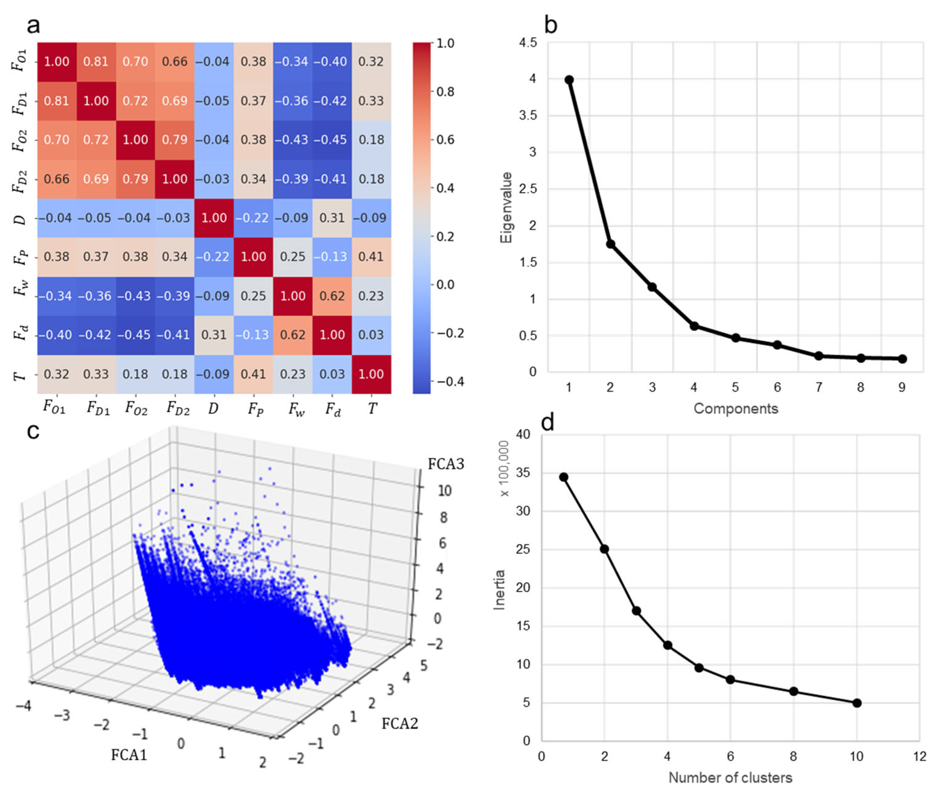
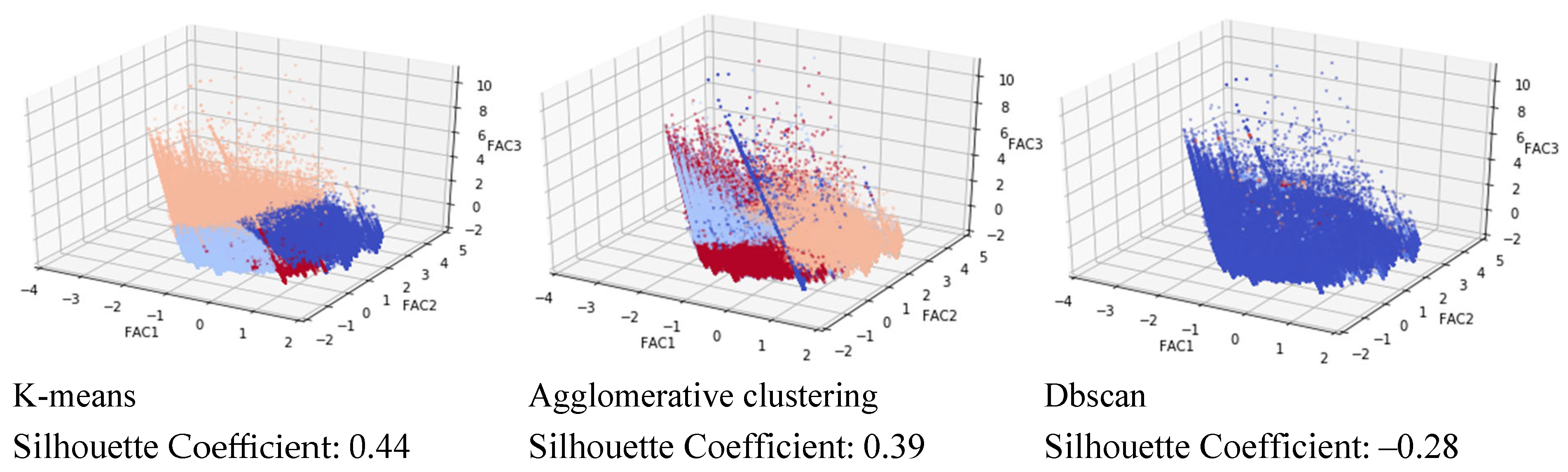
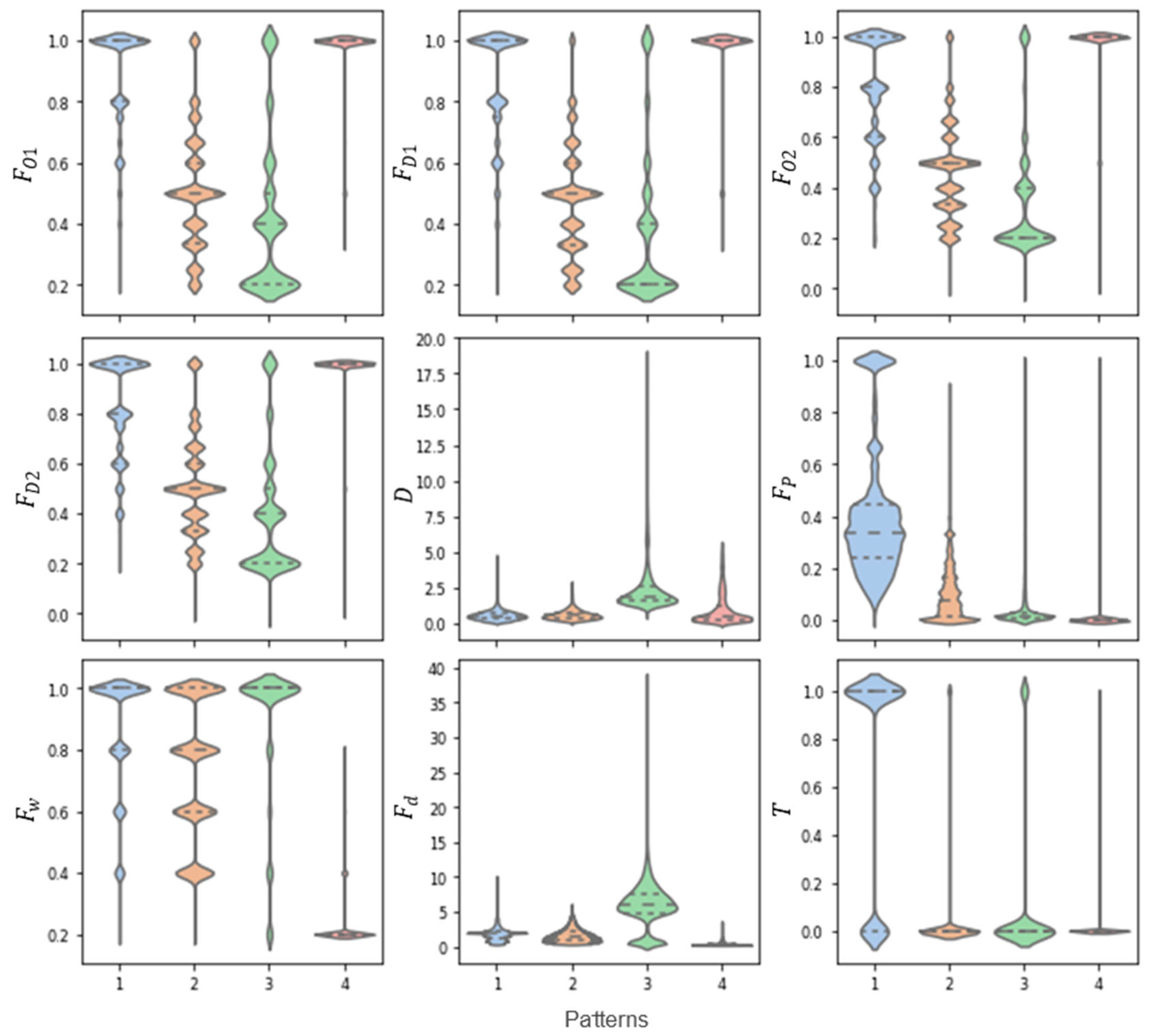
3.2.1. Results of Clustering: Dimensionality Reduction and Clustering Outcomes

As shown in Figure 3a, there are strong correlations among the features, particularly among the stability coefficients $F_{O1}$, $F_{O1}$, $F_{D1}$, and $F_{D2}$. Consequently, dimensionality reduction was necessary for the feature variables. Prior to dimensionality reduction, the experimental results yielded a KMO value of 0.78 (greater than 0.5) and a Bartlett’s test of sphericity p-value of 0.000 (less than 0.05), indicating that the dataset was suitable for dimensionality reduction. As illustrated in Figure 3b, three variables had eigenvalues greater than 1, and the cumulative variance explained by these three principal components reached 77%, effectively capturing the variability in all features. Therefore, three latent variables were extracted from the nine original feature variables after dimensionality reduction. The three-dimensional latent variables obtained through dimensionality reduction are presented in Figure 3c. Finally, the optimal number of travel behavior patterns was determined to be four based on the elbow method, as shown in Figure 3d.

Based on the method described in Section 2.1.2, we obtained clustering results using three different clustering methods, as shown in Figure 4. The silhouette coefficients for the three clustering methods are 0.44, 0.39, and –0.28, respectively. The K-means clustering algorithm performed the best, followed by the Agglomerative clustering algorithm. The DBSCAN algorithm is not suitable for pattern partitioning in this method, possibly due to the uneven distribution of feature indicator data.

After categorizing the travel behavior of 1,144,105 vehicles into four patterns, the distribution and probability density of spatial-temporal feature data for each pattern are presented using violin plots in Figure 5. Additionally, the average features are summarized in

Table 3. Mean Characteristics.

Travel Partterns	Fo1	Fd1	Fo2	Fd2	D	Fp	Fw	Fd	T
1	0.88	0.86	0.79	0.81	0.28	0.4	0.86	2.09	0.68
2	0.51	0.47	0.46	0.51	0.30	0.1	0.74	2.18	0.04
3	0.42	0.37	0.36	0.41	1.16	0.04	0.89	6.66	0.1
4	0.98	0.97	0.98	0.98	0.49	0.02	0.22	1.59	0

. Figure 5 illustrates that stability indicators $F_{O1}$, $F_{O1}$, $F_{D1}$, and $F_{D2}$ exhibit similar distributions, with multiple peaks observed for patterns 1, 2, and 3, while pattern 4 follows a logarithmic normal distribution. Table 3 reveals minor differences in the averages of $F_{O1}$, $F_{O1}$, $F_{D1}$, and $F_{D2}$, with patterns 1 and 4 exhibiting high stability at the beginning and end points, pattern 2 at a medium level, and pattern 3 at the lowest level. Notably, pattern 3 displays a logarithmic normal distribution, with the highest average trip distance, $D$, followed by pattern 4, pattern 2, and pattern 1. The similarity distribution of travel paths, $F_p$, differs across patterns, with pattern 1 exhibiting a peak distribution pattern and patterns 2, 3, and 4 displaying unimodal distributions. Pattern 1 has the highest path similarity, with consistent daily travel paths, while pattern 2 shows lower path similarity, and patterns 3 and 4 have nearly non-repeating travel paths. Regarding weekday travel stability coefficients, $F_w$, patterns 1 to 3 show concentrated distributions around 1, indicating almost daily travel, while pattern 2 travels approximately 2–5 days a week, and pattern 4 primarily travels only one day a week. Furthermore, pattern 3 has the highest average daily travel frequency, $F_d$, followed by patterns 1 and 2, which remain stable at around 2 times, while pattern 4 exhibits a daily average travel frequency of approximately 1 to 2 times, representing the lowest travel frequency. In terms of travel time stability, pattern 1 is significantly more stable than the other categories, while pattern 3 displays lower time stability, and patterns 2 and 4 are relatively unconstrained by time.

In summary, pattern 1 shows relatively stable starting and ending points for trips, with consistent weekday travel and a high frequency of daily trips. These trips typically follow fixed routes, with strong time constraints on the first trip of the day and tend to be short-distance travels. These characteristics align with commuting patterns.

Pattern 2 exhibits moderate stability in starting and ending points, with weekday travel consistency and daily trip frequency similar to pattern 1. However, the trips are shorter, with less route repetition and no clear time constraints on departure. These trips lack a defined purpose, fitting the irregular travel pattern category.

Pattern 3 shows low stability in starting and ending points but high weekday travel consistency, along with the highest average daily trip frequency and distance. There are few constraints on routes or timing, which is consistent with commercial vehicle usage patterns.

Pattern 4 displays low travel stability, with only one trip recorded during the statistical period. This results in a high level of stability in starting and ending points, suggesting a transit-related pattern.

Therefore, vehicles in Patterns 1 through 4 can be classified as Commuting Vehicles (CVs), Irregular Vehicles (IVs), Commercially Used Vehicles (CUVs), and Transit-once Vehicles (TVs), respectively.

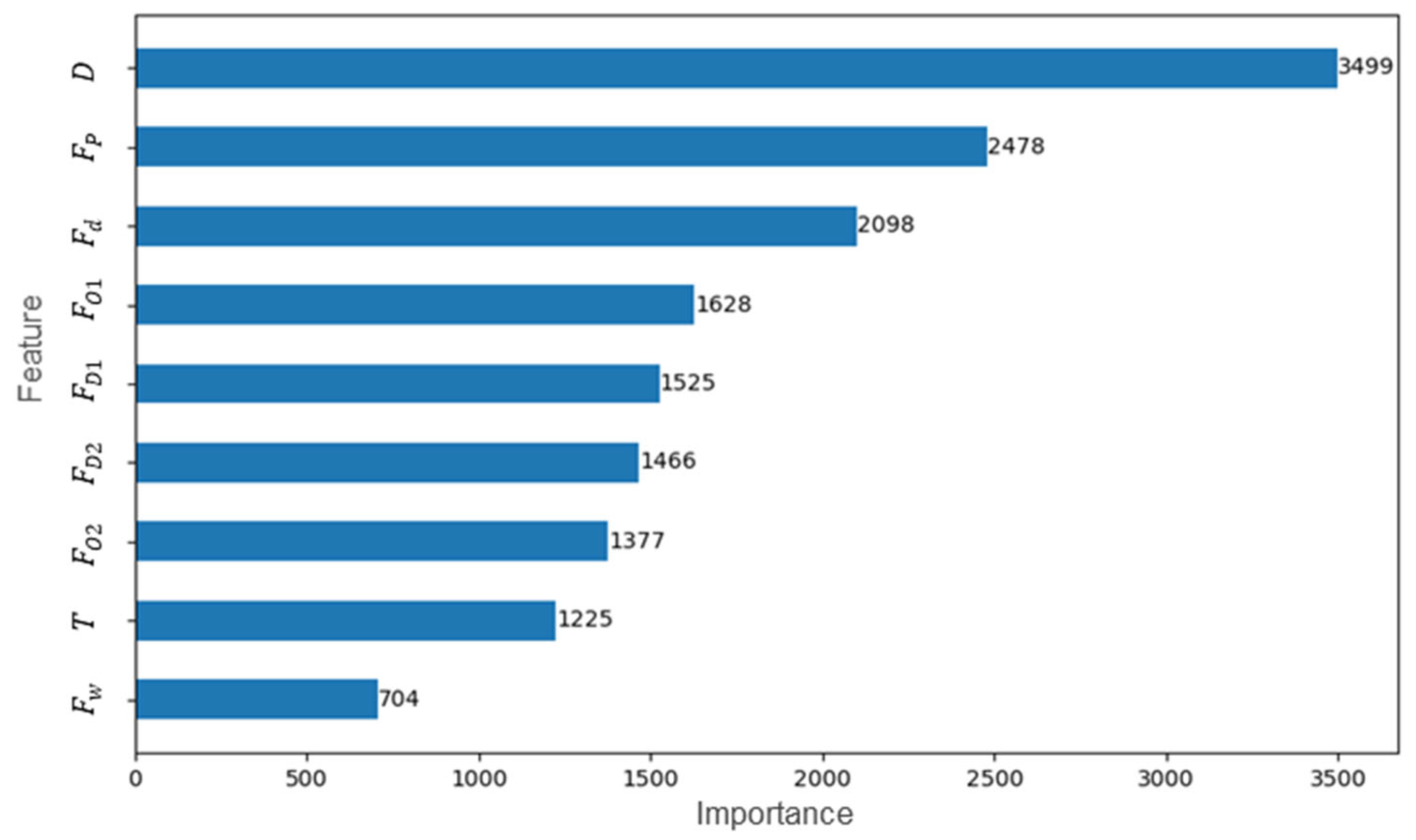
3.2.2. Recognition Results of Classification Model

Based on the pattern division results, we constructed a classification model suitable for large-scale scenarios following the method outlined in Section 2.1.3. Utilizing nine feature variables, the trained LightGBM classification model achieves an F1-score of 0.99, demonstrating high precision and efficiency in recognition. However, calculating the nine feature variables for a massive number of individuals in large-scale scenarios poses a challenge, exacerbated by the intercorrelations among these variables. Therefore, to address this issue, we ranked the feature importance, as depicted in Figure 6, and tested the impact of different feature quantities on the classification recognition performance, as shown in Figure 7.

From the experimental results, it is evident that relying solely on three feature variables, $D, F_p \mathrm{a}\mathrm{n}\mathrm{d} F_d$, achieves an F1-score of 0.87, indicating satisfactory performance of the classification model. Moreover, the importance of the four feature variables, $F_{O1}$, $F_{O1},F_{D1}\mathrm{a}\mathrm{n}\mathrm{d}{ F}_{D2}$, is similar, and utilizing only one of them yields the same result. Therefore, in large-scale scenarios, efficient recognition of vehicle travel behavior patterns can be achieved by calculating only the three feature variables, $D, F_p \mathrm{a}\mathrm{n}\mathrm{d} F_d$, and subsequently employing the trained classification model for classification.

3.3. Congestion Risk Associated with Different Travel Behavior Patterns

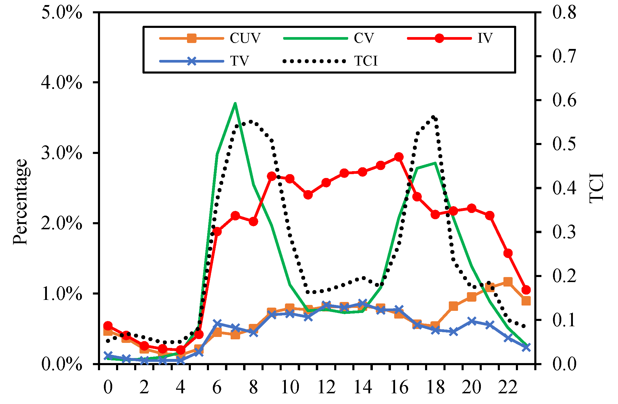
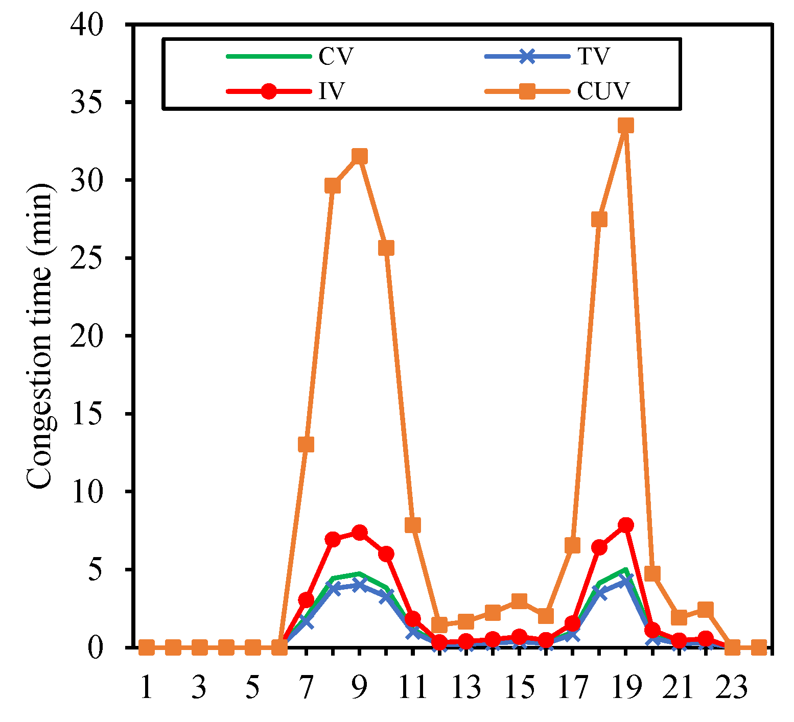
3.3.1. Time Distribution of Congestion for Each Pattern

Figure 8 illustrates the time distribution of travel for each pattern. Additionally, we employ an improved Traffic Congestion Index (TCI) to represent the overall traffic condition, as shown in Equation (19), where TCI ranges from [0, 1], with higher values indicating greater congestion.

$$TCI=1-{\displaystyle \frac{{\sum }_{i=1}^N{\frac{L_i}{V_{free\_i}}W}_i}{{\sum }_{i=1}^N{\frac{L_i}{V_i}W}_i}}$$

(19)

where $L_i$ is the length of the road segment, $W_i$ is the segment weight, $V_{free\_i}$ is the free-flow speed of the segment, and $V_i$ is the real-time speed of the segment.

From Figure 8, it can be observed that the CVs pattern peaks during morning and evening rush hours (6:00–10:00 a.m. and 4:00–8:00 p.m.), with a higher concentration in the morning compared to the evening. In contrast, the travel patterns of CUVs and TVs on expressways show the opposite trend to CVs, being lower during peak hours and higher during off-peak hours, with CUVs exhibiting increased activity during the evening (7:00–11:00 p.m.). IVs activity is primarily concentrated between 9:00 a.m. and 4:00 p.m. The trend in the road congestion index aligns with the changes in CVs travel volume, suggesting that the surge in CV traffic directly contributes to road congestion. When CVs’ travel volume peaks, road congestion also reaches its highest point. Does this imply that the congestion risk for CVs is the highest? The answer is negative.

Additionally, Figure 9 and Figure 10, respectively, present the distribution of congestion duration and the daily average congestion duration for each travel behavior pattern. The highest congestion risk is not concentrated in CV patterns during peak hours, but rather in CUV patterns that seek to avoid peak-hour travel. Despite accounting for only 15.17% of the total, CUV patterns can experience congestion for up to three hours a day, with nearly half of this time spent in congested conditions during peak hours. Hence, CUV drivers intentionally avoid peak hours, preferring to engage in activities such as shift changes and meals during these times, rather than being stuck in traffic. This also explains why the volume of CUV travel during peak hours in Figure 9 is lower than during off-peak hours. Similarly, TV patterns also avoid peak-hour travel, while IVs patterns, although not extensively avoiding peak-hour travel, exhibit a slower growth in travel volume during the morning peak period. The second-highest congestion risk is observed in the most prevalent IV patterns, followed by CV patterns, with TV patterns having the lowest congestion risk. Although congestion often occurs during peak hours, the congestion risk for CV patterns, which are concentrated during peak hours, is comparatively low.

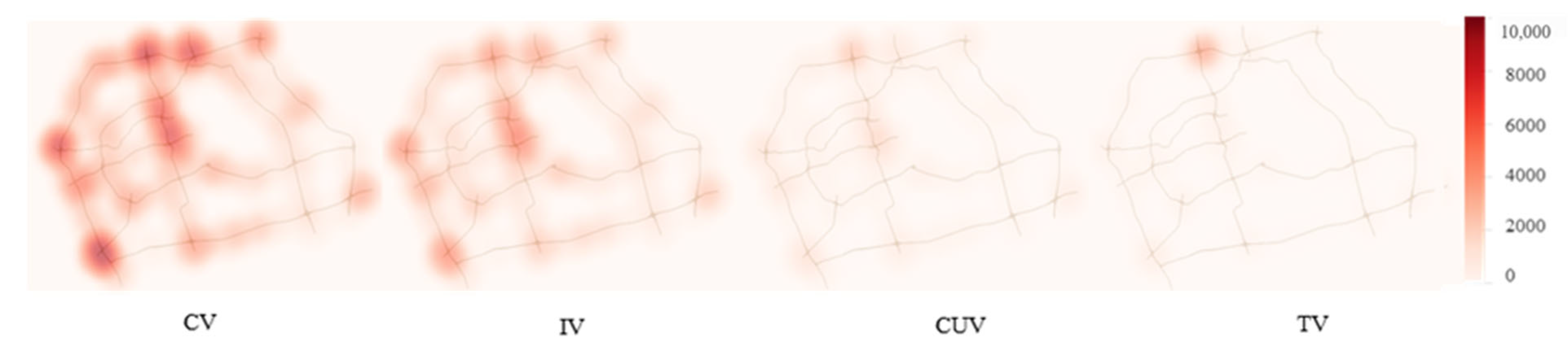
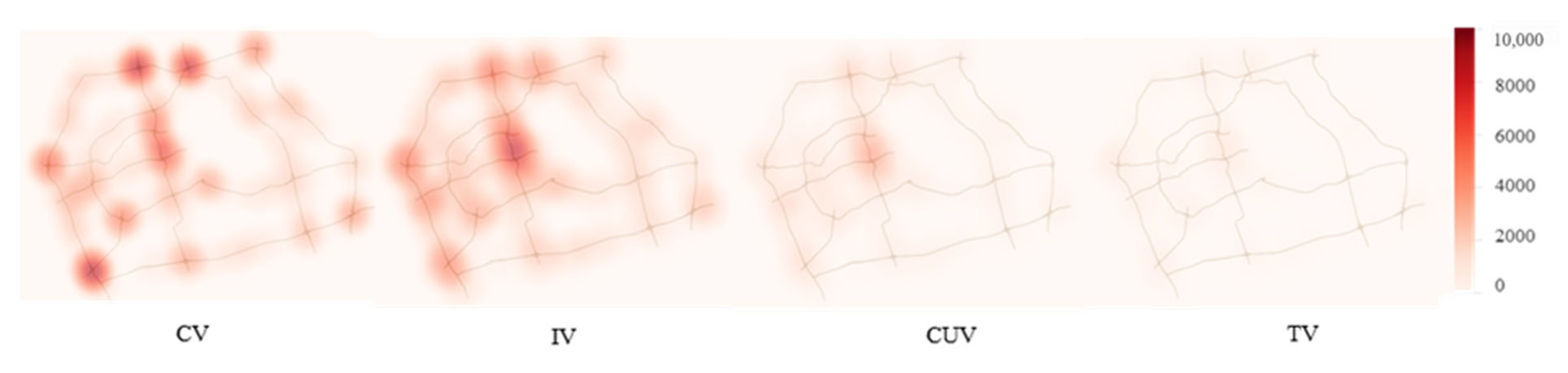
3.3.2. Spatial Distribution of Congestion for Each Pattern

Figure 11 and Figure 12 show the kernel density estimates of travel routes for different travel patterns. These figures clearly indicate that congestion occurs at varying locations for each pattern, with congestion points shifting across different time periods. CV patterns experience congestion primarily on the outer ring and in the city center, suggesting that commuters may live on the outer ring and work in the city center. During the morning peak, CV patterns show a higher concentration on expressways compared to the evening peak. This can be attributed to two factors: commuters tend to have relatively consistent working hours but varying off-duty hours and they prefer expressways in the morning to minimize travel time, while they enjoy more flexibility in route choice after work. For TV patterns, the concentration during the morning peak is also higher than in the evening, with their activities mainly concentrated on the outer ring and passing through the area. In contrast, IV and CUV patterns exhibit higher activity levels during the evening peak, as people tend to engage more in dining, entertainment, and leisure activities, which increases the activity of these patterns. Moreover, leisure and entertainment facilities are predominantly located in the city center, leading to higher concentrations of IV and CUV patterns in this area.

Furthermore, the congestion points of IV and CV patterns overlap significantly, suggesting similarities or a high degree of commonality in their travel routes. CUV patterns only overlap with CV patterns in the city center, while TVs patterns overlap with CVs patterns on the outer ring.

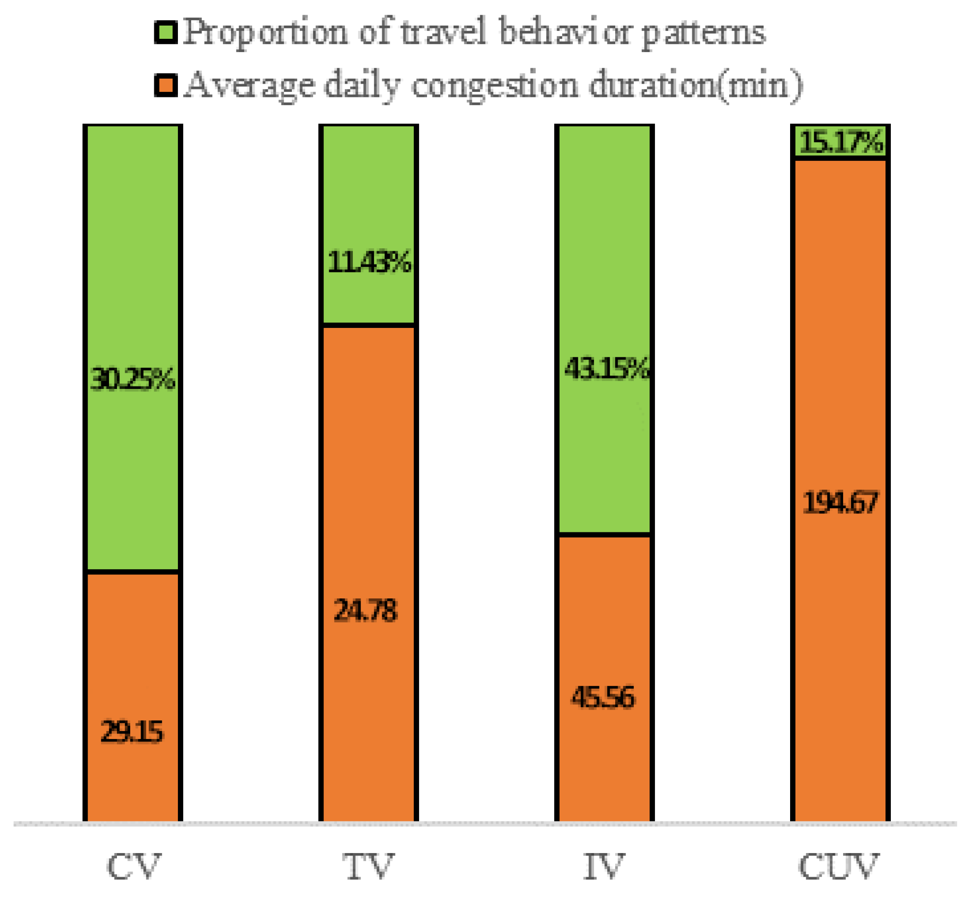
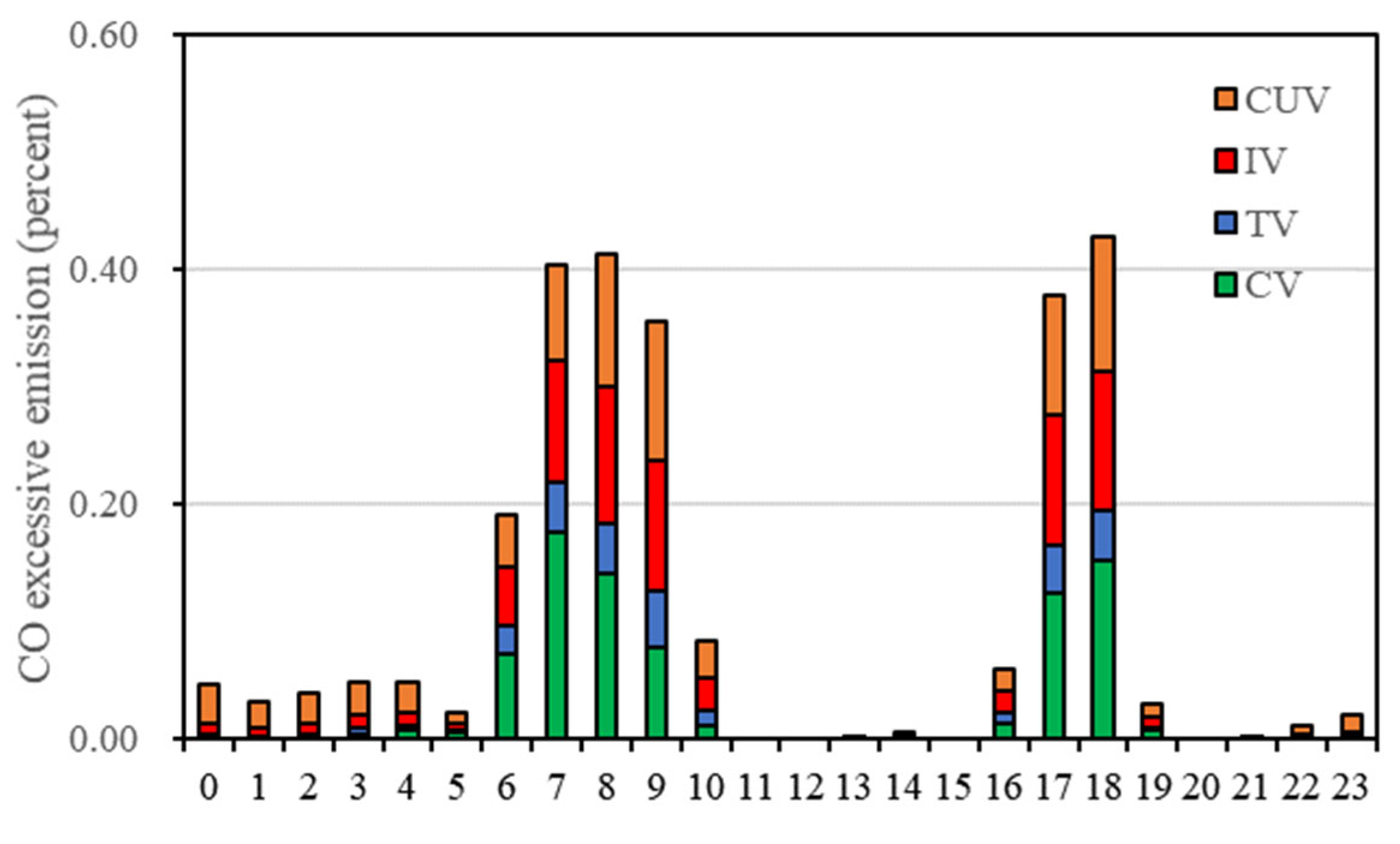
3.4. Excessive Emissions from Various Patterns

To investigate the additional emissions generated by various patterns during congestion, we explored the excessive emissions of CO. CO emissions associated with traffic are mainly released during vehicle acceleration and deceleration over short periods, which are more relevant in the context of traffic congestion because vehicles involved in congested traffic must accelerate and decelerate frequently [48].

Figure 13 illustrates the distribution of excessive emissions for each pattern. Excessive CO emissions exhibit a trend consistent with the overall traffic flow, showing a bimodal distribution. During the morning peak hours, CO emissions from congestion account for 41% of the total emissions, while during the evening peak, they account for 43%. An interesting phenomenon is that CUVs, accounting for only 15.17% of the total, and IVs, accounting for 43.15%, produce nearly the same amount of excessive CO emissions during peak hours. Although CVs patterns rank third in terms of congestion duration, they have the largest excessive CO emissions. This indicates that commuters do not perceive congestion as significantly as other travelers, but their gas pollution is the largest.

4. Discussion

4.1. Discussion on the Spatiotemporal Characteristics and Congestion Risks of Various Patterns

In this study, we examined travel behavior patterns and their associated congestion risks using large-scale LPR data. We demonstrated that it is possible to classify a large fleet of vehicles (1,144,105 vehicles) based on just three travel characteristics: daily travel frequency, path similarity, and average daily travel distance. Previous studies have relied on more complex indicators, such as “residential points, work points, distance ratios, maximum route similarity, actual driving distance, vehicle usage intensity, driving regularity, regular trips, and time patterns”. In contrast, our approach is simpler, provides a more comprehensive classification, and is more scalable for large-scale vehicle identification. Moreover, we included estimates of congestion risks and excessive emissions for each mode, an aspect that previous studies have not addressed [5,49].

We classified vehicles into four categories: Commercially Used Vehicles (CUVs), Commuting Vehicles (CVs), Irregular Vehicles (IVs), and Transit-once Vehicles (TVs). Among these, CVs exhibited strong spatiotemporal stability, consistent with prior research. On average, CVs traveled twice daily on weekdays, with stable departure times (fluctuations within 30 min, primarily concentrated during morning rush hours), consistent commuting routes (using the same route daily), and short to medium travel distances. CUVs, on the other hand, exhibited high daily travel frequency and longer travel distances, characteristics commonly associated with commercial vehicles in existing studies. IVs, while exhibiting travel frequency and distance similar to CVs, lacked spatiotemporal stability, resembling non-commuting family vehicles. TVs, characterized by infrequent travel, showed no spatiotemporal stability. To validate the accuracy of these classifications, we obtained trajectory data for 23,352 commercial taxis from relevant management departments. Using our method, we successfully identified 19,709 vehicles as CUVs, achieving an accuracy rate of 85%.

Regarding congestion risk and emissions, the congestion risks for all travel modes followed a bimodal distribution, consistent with the tidal patterns observed in traffic flow and corroborated by existing research [43].

4.2. Discussion on Strategies to Reduce Congestion Risks

By identifying travel patterns and estimating congestion risks, relevant authorities can develop targeted strategies to manage demand and effectively reduce congestion. This paper evaluates the contribution of each travel pattern to congestion, with the following proportions: CUVs (15.17%), CVs (30.25%), IVs (43.15%), and TVs (11.43%). The data indicate that approximately 12.6% of road congestion during peak hours results from overload, meaning that 87.4% of travel demand can be accommodated, while the remaining 12.6% contributes to congestion. Although different vehicles may follow distinct travel patterns, they all have equal rights to access the road. Thus, completely restricting certain vehicle types, such as CUVs or TVs, from entering expressways during peak hours may raise concerns.

Furthermore, different travel patterns have varying route scopes. For instance, banning CUVs from expressways may not alleviate congestion on outer loops. Each pattern also presents different congestion risks and emission levels. While current research often focuses on CVs, commuting vehicles typically do not face high congestion risks. In contrast, CUVs, which receive less attention, encounter significant congestion risks and generate higher emissions. Therefore, congestion management strategies should account for the diverse travel characteristics of each pattern and integrate them accordingly. Focusing solely on a specific vehicle type is insufficient.

The surge of CVs during peak hours is one of the direct causes of congestion. If at least 12.6% of vehicles can be dispersed during peak hours, reducing the concentration of vehicles in the same spatiotemporal space, congestion relief can be achieved. Moreover, with economic development, the number of motor vehicles will only increase in the future. The proportion of “conservative” car owners who primarily use cars for all their travel will rise [50], and their willingness to use shared mobility or public transportation will remain low [51,52,53,54]. A large-scale shift from private car travel to public transportation will still require a long transitional period. Nevertheless, the vigorous development of public transportation remains a key strategy for alleviating traffic congestion in the future. At the same time, spatiotemporal guidance of vehicles across different travel modes is also an efficient and equitable strategy [55,56]. Based on the spatiotemporal characteristics of various modes, guiding travelers in terms of time or space can help alleviate network congestion. For example, path preferences can directly assist traffic managers in identifying more feasible and effective route planning solutions [57,58,59]. Alternatively, travelers gathered during peak periods can be subject to time-based guidance [39,57,58,59,60,61]. Targeted control of the most congested travelers can maximize congestion and emission reduction [62,63,64,65].

5. Conclusions

This study investigates congestion risks and excess emissions associated with various travel behavior patterns using comprehensive LPR data from urban expressways. First, we propose a pattern recognition method based on the spatiotemporal information embedded in LPR data, designed for large-scale applications. We then analyze the spatiotemporal characteristics of different travel patterns, examining their corresponding traffic congestion risks and excess emissions. Significant differences in congestion risk and duration distributions were found across the different travel modes. The study revealed that the sharp increase in travel volume associated with CVs is the primary cause of road congestion. Despite CVs having the highest travel volume during peak periods, they do not exhibit the highest congestion risk. In fact, CUVs, which avoid peak hours, show a higher congestion risk. The congestion duration for CUVs during peak periods can extend up to three hours, with nearly half of the peak period spent in congestion. IVs rank second in terms of congestion risk, followed by CVs, while TVs experience the least congestion risk. Further analysis revealed distinct travel routes and congestion points for the various modes. Congestion for CVs predominantly occurs on the urban outer ring road and in city centers, reflecting the distribution of commuters’ homes and workplaces. IVs and CUVs, in contrast, primarily operate within city centers.

Excessive CO emissions followed a similar bimodal distribution pattern to traffic flow, with peak emissions occurring during the morning (41% of total excessive CO emissions) and evening (43%). Interestingly, although CUVs account for only 15.17% of the total fleet, their excessive CO emissions during peak periods are nearly identical to those of IVs, which make up 43.15% of the fleet. This discrepancy reflects the emission overage caused by congestion for CUVs during peak times. Notably, although the CV mode ranks third in terms of congestion duration during peak periods, it generates the highest levels of excessive CO emissions. This suggests that, despite CV drivers’ lower sensitivity to congestion, their emissions during peak periods have a disproportionately negative environmental impact. In conclusion, the relationship between congestion risk and emissions varies across different travel modes, especially during peak periods when the differences in emissions are more pronounced. Future traffic management strategies should consider the specific characteristics of each mode, particularly in terms of emission control during peak times, to reduce both traffic congestion and environmental pollution.

This research enhances our understanding of the relationship between individual travel behavior and traffic congestion, providing valuable insights for personal travel time planning and health management. Furthermore, the methodology and conclusions presented in this paper can inform the development of personalized, proactive traffic demand management strategies. This study does have some limitations. Firstly, to analyze congestion risks and emissions associated with various travel patterns, only weekday data were considered, and weekend travel patterns were not examined. Secondly, while we proposed a comprehensive framework for pattern classification and recognition, this study focused only on expressway networks and did not include the entire urban road network. As a result, some vehicle trajectories may not fully represent travel records. In the future, we plan to collect data from a broader spatiotemporal scope to further enhance the study of travel patterns. We also intend to explore route induction under different travel pattern classifications.

References

1. Sandow, E.; Westerlund, O.; Lindgren, U. Is Your Commute Killing You? On the Mortality Risks of Long-Distance Commuting. Environ. Plan. Econ. Space 2014, 46, 1496–1516. [Google Scholar] [CrossRef]
2. Currie, J.; Walker, R. Traffic Congestion and Infant Health: Evidence from E-ZPass. Am. Econ. J. Appl. Econ. 2011, 3, 65–90. [Google Scholar] [CrossRef]
3. Bigazzi, A.Y.; Figliozzi, M.A.; Clifton, K.J. Traffic Congestion and Air Pollution Exposure for Motorists: Comparing Exposure Duration and Intensity. Int. J. Sustain. Transp. 2015, 9, 443–456. [Google Scholar] [CrossRef]
4. Wu, W.; Wang, M.; Zhang, F. Commuting Behavior and Congestion Satisfaction: Evidence from Beijing, China. Transp. Res. Part Transp. Environ. 2019, 67, 553–564. [Google Scholar] [CrossRef]
5. Deng, J.; Cui, Y.; Chen, X.; Bachmann, C.; Yuan, Q. Who Are on the Road? A Study on Vehicle Usage Characteristics Based on One-Week Vehicle Trajectory Data. Int. J. Digit. Earth 2023, 16, 1962–1984. [Google Scholar] [CrossRef]
6. Cohen, A.P.; Shaheen, S.A.; Farrar, E.M. Urban Air Mobility: History, Ecosystem, Market Potential, and Challenges. IEEE Trans. Intell. Transp. Syst. 2021, 22, 6074–6087. [Google Scholar] [CrossRef]
7. Coppola, P.; De Fabiis, F.; Silvestri, F. Urban Air Mobility Passengers’ Profiling: Evidence from Milan Airports, Italy. Transp. Res. Rec. J. Transp. Res. Board 2024. [Google Scholar] [CrossRef]
8. Karami, H.; Abbasi, M.; Samadzad, M.; Karami, A. Unraveling Behavioral Factors Influencing the Adoption of Urban Air Mobility from the End User’s Perspective in Tehran—A Developing Country Outlook. Transp. Policy 2024, 145, 74–84. [Google Scholar] [CrossRef]
9. Yang, J.; Wang, Y.; Hang, X.; Delahaye, D. A Review on Airspace Design and Risk Assessment for Urban Air Mobility. IEEE Access 2024, 12, 157599–157611. [Google Scholar] [CrossRef]
10. Qiao, X.; Chen, G.; Lin, W.; Zhou, J. The Impact of Battery Performance on Urban Air Mobility Operations. Aerospace 2023, 10, 631. [Google Scholar] [CrossRef]
11. Lindsey, R.; de Palma, A.; Rezaeinia, P. Tolls vs Tradable Permits for Managing Travel on a Bimodal Congested Network with Variable Capacities and Demands. Transp. Res. Part C Emerg. Technol. 2023, 148, 104028. [Google Scholar] [CrossRef]
12. Krabbenborg, L.; Molin, E.; Annema, J.A.; van Wee, B. Public Frames in the Road Pricing Debate: A Q-Methodology Study. Transp. Policy 2020, 93, 46–53. [Google Scholar] [CrossRef]
13. Macioszek, E.; Granà, A.; Fernandes, P.; Coelho, M.C. New Perspectives and Challenges in Traffic and Transportation Engineering Supporting Energy Saving in Smart Cities—A Multidisciplinary Approach to a Global Problem. Energies 2022, 15, 4191. [Google Scholar] [CrossRef]
14. Khorram Dehnavi, S.; MorovatiSharifabadi, A.; AghidiKheyrabadi, S.; HosseiniBamakan, S.M. Evaluating Private Car Users’ Preference to Congestion Pricing: A Study on Trip Cancellation Behavior. Case Stud. Transp. Policy 2024, 18, 101300. [Google Scholar] [CrossRef]
15. Wang, R.; Zhou, M.; Gao, K.; Alabdulwahab, A.; Rawa, M.J. Personalized Route Planning System Based on Driver Preference. Sensors 2022, 22, 11. [Google Scholar] [CrossRef] [PubMed]
16. Zhang, Z.; Li, M. Finding Paths With Least Expected Time in Stochastic Time-Varying Networks Considering Uncertainty of Prediction Information. IEEE Trans. Intell. Transp. Syst. 2023, 24, 14362–14377. [Google Scholar] [CrossRef]
17. Dong, Y.; Wang, S.; Li, L.; Zhang, Z. An Empirical Study on Travel Patterns of Internet Based Ride-Sharing. Transp. Res. Part C Emerg. Technol. 2018, 86, 1–22. [Google Scholar] [CrossRef]
18. Chen, X.; Zahiri, M.; Zhang, S. Understanding Ridesplitting Behavior of On-Demand Ride Services: An Ensemble Learning Approach. Transp. Res. Part C Emerg. Technol. 2017, 76, 51–70. [Google Scholar] [CrossRef]
19. Wang, F.; Wang, J.; Cao, J.; Chen, C.; Ban, X. (Jeff). Extracting Trips from Multi-Sourced Data for Mobility Pattern Analysis: An App-Based Data Example. Transp. Res. Part C Emerg. Technol. 2019, 105, 183–202. [Google Scholar] [CrossRef]
20. Badiola, N.; Raveau, S.; Galilea, P. Modelling Preferences towards Activities and Their Effect on Departure Time Choices. Transp. Res. Part Policy Pract. 2019, 129, 39–51. [Google Scholar] [CrossRef]
21. Rahman, M.; Akther, S. Intercity Commuting in Metropolitan Regions: A Mode Choice Analysis of Commuters Traveling to Dhaka from Nearby Cities. J. Urban Plan. Dev. 2022, 148, 05021060. [Google Scholar] [CrossRef]
22. Rafiq, R.; McNally, M.G. A Structural Analysis of the Work Tour Behavior of Transit Commuters. Transp. Res. Part Policy Pract. 2022, 160, 61–79. [Google Scholar] [CrossRef]
23. Jiang, S.; Yang, Y.; Gupta, S.; Veneziano, D.; Athavale, S.; González, M.C. The TimeGeo Modeling Framework for Urban Motility without Travel Surveys. Proc. Natl. Acad. Sci. USA 2016, 113, E5370–E5378. [Google Scholar] [CrossRef]
24. Chen, H.; Cai, M.; Xiong, C. Research on Human Travel Correlation for Urban Transport Planning Based on Multisource Data. Sensors 2021, 21, 195. [Google Scholar] [CrossRef] [PubMed]
25. Guo, Y.; Yang, F.; Yan, H.; Xie, S.; Liu, H.; Dai, Z. Activity-Based Model Based on Multi-Day Cellular Data: Considering the Lack of Personal Attributes and Activity Type. IET Intell. Transp. Syst. 2023, 17, 2474–2492. [Google Scholar] [CrossRef]
26. Zheng, Y.; Capra, L.; Wolfson, O.; Yang, H. Urban Computing: Concepts, Methodologies, and Applications. ACM Trans. Intell. Syst. Technol. 2014, 5, 1–55. [Google Scholar] [CrossRef]
27. Li, Z.; Xiong, G.; Wei, Z.; Zhang, Y.; Zheng, M.; Liu, X.; Tarkoma, S.; Huang, M.; Lv, Y.; Wu, C. Trip Purposes Mining from Mobile Signaling Data. IEEE Trans. Intell. Transp. Syst. 2022, 23, 13190–13202. [Google Scholar] [CrossRef]
28. Chen, Y.; Wang, Z.; Sun, H.; Wang, J. Exploring Activity Patterns and Trip Purposes of Public Transport Passengers from Smart Card Data. J. Transp. Eng. Part Syst. 2023, 149, 04023076. [Google Scholar] [CrossRef]
29. Liu, Z.; Li, R.; Wang, X.; Shang, P. Effects of Vehicle Restriction Policies: Analysis Using License Plate Recognition Data in Langfang, China. Transp. Res. Part Policy Pract. 2018, 118, 89–103. [Google Scholar] [CrossRef]
30. Chang, Y.; Duan, Z.; Yang, D. Using ALPR Data to Understand the Vehicle Use Behaviour under TDM Measures. IET Intell. Transp. Syst. 2018, 12, 1264–1270. [Google Scholar] [CrossRef]
31. Goulet-Langlois, G.; Koutsopoulos, H.N.; Zhao, Z.; Zhao, J. Measuring Regularity of Individual Travel Patterns. IEEE Trans. Intell. Transp. Syst. 2018, 19, 1583–1592. [Google Scholar] [CrossRef]
32. Sun, L.; Chen, X.; He, Z.; Miranda-Moreno, L.F. Routine Pattern Discovery and Anomaly Detection in Individual Travel Behavior. Netw. Spat. Econ. 2023, 23, 407–428. [Google Scholar] [CrossRef]
33. Yao, W.; Zhang, M.; Jin, S.; Ma, D. Understanding Vehicles Commuting Pattern Based on License Plate Recognition Data. Transp. Res. Part C Emerg. Technol. 2021, 128, 103142. [Google Scholar] [CrossRef]
34. Wan, L.; Tang, J.; Wang, L.; Schooling, J. Understanding Non-Commuting Travel Demand of Car Commuters—Insights from ANPR Trip Chain Data in Cambridge. Transp. Policy 2021, 106, 76–87. [Google Scholar] [CrossRef]
35. Berrill, P.; Nachtigall, F.; Javaid, A.; Milojevic-Dupont, N.; Wagner, F.; Creutzig, F. Comparing Urban Form Influences on Travel Distance, Car Ownership, and Mode Choice. Transp. Res. Part Transp. Environ. 2024, 128, 104087. [Google Scholar] [CrossRef]
36. Lian, T.; Loo, B.P.Y. Cost of Travel Delays Caused by Traffic Crashes. Commun. Transp. Res. 2024, 4, 100124. [Google Scholar] [CrossRef]
37. Higgins, C.D.; Sweet, M.N.; Kanaroglou, P.S. All Minutes Are Not Equal: Travel Time and the Effects of Congestion on Commute Satisfaction in Canadian Cities. Transportation 2018, 45, 1249–1268. [Google Scholar] [CrossRef]
38. Beland, L.-P.; Brent, D.A. Traffic and Crime. J. Public Econ. 2018, 160, 96–116. [Google Scholar] [CrossRef]
39. Yildirimoglu, M.; Ramezani, M.; Amirgholy, M. Staggered Work Schedules for Congestion Mitigation: A Morning Commute Problem. Transp. Res. Part C Emerg. Technol. 2021, 132, 103391. [Google Scholar] [CrossRef]
40. Ravalet, E.; Rérat, P. Teleworking: Decreasing Mobility or Increasing Tolerance of Commuting Distances? Built Environ. 2019, 45, 582–602. [Google Scholar] [CrossRef]
41. Alessandretti, L.; Lehmann, S. Trip Frequency Is Key Ingredient in New Law of Human Travel. Nature 2021, 593, 515–516. [Google Scholar] [CrossRef]
42. Warne, R.T.; Larsen, R. Evaluating a Proposed Modification of the Guttman Rule for Determining the Number of Factors in an Exploratory Factor Analysis. Psychol. Test Assess. Model. 2014, 56, 104–123. [Google Scholar]
43. Kan, Z.; Kwan, M.-P.; Liu, D.; Tang, L.; Chen, Y.; Fang, M. Assessing Individual Activity-Related Exposures to Traffic Congestion Using GPS Trajectory Data. J. Transp. Geogr. 2022, 98, 103240. [Google Scholar] [CrossRef]
44. Yang, D.; Zhang, S.; Niu, T.; Wang, Y.; Xu, H.; Zhang, K.M.; Wu, Y. High-Resolution Mapping of Vehicle Emissions of Atmospheric Pollutants Based on Large-Scale, Real-World Traffic Datasets. Atmos. Chem. Phys. 2019, 19, 8831–8843. [Google Scholar] [CrossRef]
45. Wu, Y.; Zhang, S.; Hao, J.; Liu, H.; Wu, X.; Hu, J.; Walsh, M.P.; Wallington, T.J.; Zhang, K.M.; Stevanovic, S. On-Road Vehicle Emissions and Their Control in China: A Review and Outlook. Sci. Total Environ. 2017, 574, 332–349. [Google Scholar] [CrossRef] [PubMed]
46. Zhang, S.; Wu, Y.; Huang, R.; Wang, J.; Yan, H.; Zheng, Y.; Hao, J. High-Resolution Simulation of Link-Level Vehicle Emissions and Concentrations for Air Pollutants in a Traffic-Populated Eastern Asian City. Atmos. Chem. Phys. 2016, 16, 9965–9981. [Google Scholar] [CrossRef]
47. Chen, H.; Yang, C.; Xu, X. Clustering Vehicle Temporal and Spatial Travel Behavior Using License Plate Recognition Data. J. Adv. Transp. 2017, 2017, e1738085. [Google Scholar] [CrossRef]
48. Zhang, K.; Batterman, S.; Dion, F. Vehicle Emissions in Congestion: Comparison of Work Zone, Rush Hour and Free-Flow Conditions. Atmos. Environ. 2011, 45, 1929–1939. [Google Scholar] [CrossRef]
49. Chen, X.; Li, K.; Zhang, H.; Yuan, Q.; Ye, Q. Identifying and Recognizing Usage Pattern of Electric Vehicles Using GPS and On-Board Diagnostics Data. In Proceedings of the International Conference on Transportation and Development 2020, Seattle, WA, USA, 26–29 May 2020; pp. 85–97. [Google Scholar] [CrossRef]
50. Baro, R.; Rao, K.V.K.; Velaga, N.R. Role of Private Vehicle Commuters’ Travel Wellbeing Perception in Mode Shift Behavior towards an Upcoming Metro in Mumbai Metropolitan Region. Case Stud. Transp. Policy 2024, 16, 101210. [Google Scholar] [CrossRef]
51. Li, W.; Kamargianni, M. Steering Short-Term Demand for Car-Sharing: A Mode Choice and Policy Impact Analysis by Trip Distance. Transportation 2020, 47, 2233–2265. [Google Scholar] [CrossRef]
52. van ’t Veer, R.; Annema, J.A.; Araghi, Y.; Homem de Almeida Correia, G.; van Wee, B. Mobility-as-a-Service (MaaS): A Latent Class Cluster Analysis to Identify Dutch Vehicle Owners’ Use Intention. Transp. Res. Part Policy Pract. 2023, 169, 103608. [Google Scholar] [CrossRef]
53. Wei, B.; Zhang, X.; Liu, W.; Saberi, M.; Waller, S.T. Capacity Allocation and Tolling-Rewarding Schemes for the Morning Commute with Carpooling. Transp. Res. Part C Emerg. Technol. 2022, 142, 103789. [Google Scholar] [CrossRef]
54. Lavieri, P.S.; Bhat, C.R. Modeling Individuals’ Willingness to Share Trips with Strangers in an Autonomous Vehicle Future. Transp. Res. Part Policy Pract. 2019, 124, 242–261. [Google Scholar] [CrossRef]
55. Zhang, Y.; Zhao, H.; Jiang, R. Manage Morning Commute for Household Travels with Parking Space Constraints. Transp. Res. Part E Logist. Transp. Rev. 2024, 185, 103504. [Google Scholar] [CrossRef]
56. Feng, X.; Lin, Q.; Jia, N.; Tian, J. The Actual Impact of Ride-Splitting: An Empirical Study Based on Large-Scale GPS Data. Transp. Policy 2024, 147, 94–112. [Google Scholar] [CrossRef]
57. Zhu, Z.; Xie, J.; Wang, Z. Global Dynamic Path Planning Based on Fusion of A* Algorithm and Dynamic Window Approach. In Proceedings of the 2019 Chinese Automation Congress (CAC), Hangzhou, China, 22–24 November 2019; pp. 5572–5576. [Google Scholar] [CrossRef]
58. Cheng, Q.; Chen, Y.; Liu, Z. A Bi-Level Programming Model for the Optimal Lane Reservation Problem. Expert Syst. Appl. 2022, 189, 116147. [Google Scholar] [CrossRef]
59. Li, X.; Yang, H.; Ke, J. Booking Cum Rationing Strategy for Equitable Travel Demand Management in Road Networks. Transp. Res. Part B Methodol. 2023, 167, 261–274. [Google Scholar] [CrossRef]
60. Thorhauge, M.; Vij, A.; Cherchi, E. Heterogeneity in Departure Time Preferences, Flexibility and Schedule Constraints. Transportation 2021, 48, 1865–1893. [Google Scholar] [CrossRef]
61. Deng, J.; Li, T.; Yang, Z.; Yuan, Q.; Chen, X. Heterogeneity in Route Choice during Peak Hours: Implications on Travel Demand Management. Travel Behav. Soc. 2025, 38, 100922. [Google Scholar] [CrossRef]
62. Chaudhry, S.K.; Elumalai, S.P. Assessment of Sustainable School Transport Policies on Vehicular Emissions Using the IVE Model. J. Clean. Prod. 2024, 434, 140437. [Google Scholar] [CrossRef]
63. Abbiasov, T.; Heine, C.; Sabouri, S.; Salazar-Miranda, A.; Santi, P.; Glaeser, E.; Ratti, C. The 15-Minute City Quantified Using Human Mobility Data. Nat. Hum. Behav. 2024, 8, 445–455. [Google Scholar] [CrossRef] [PubMed]
64. Zong, F.; Zeng, M.; Li, Y.-X. Congestion Pricing for Sustainable Urban Transportation Systems Considering Carbon Emissions and Travel Habits. Sustain. Cities Soc. 2024, 101, 105198. [Google Scholar] [CrossRef]
65. Geng, Y.; Zhang, X.; Gao, J.; Yan, Y.; Chen, L. Bibliometric Analysis of Sustainable Tourism Using CiteSpace. Technol. Forecast. Soc. Chang. 2024, 202, 123310. [Google Scholar] [CrossRef]
Figure 1. Research framework.
Sustainability 17 00551 g001
Figure 2. Expressway network structure.
Sustainability 17 00551 g002
Figure 3. Dimensionality reduction and cluster number determination. (a) the feature correlation heatmap; (b) the scatter plot; (c) the scatter plot of feature data after dimensionality reduction; (d) the plot showing the relationship between the number of clusters and the within-cluster sum of squares.
Sustainability 17 00551 g003
Figure 4. Clustering results.
Sustainability 17 00551 g004
Figure 5. Violin plot of spatiotemporal feature indices. Different colors in the figure represent different patterns.
Sustainability 17 00551 g005
Figure 6. Ranking of feature importance.
Sustainability 17 00551 g006
Figure 7. Performance of LightGBM algorithm trained with different numbers of features.
Sustainability 17 00551 g007
Figure 8. Time distribution of travel patterns.
Sustainability 17 00551 g008
Figure 9. Time distribution of congestion risk for each pattern.
Sustainability 17 00551 g009
Figure 10. Proportion of each pattern and daily average congestion duration.
Sustainability 17 00551 g010
Figure 11. Spatial distribution of traffic congestion during morning peak hours.
Sustainability 17 00551 g011
Figure 12. Spatial distribution of traffic congestion during evening peak hours.
Sustainability 17 00551 g012
Figure 13. Excessive emissions from various patterns.
Sustainability 17 00551 g013