Article

Hydro-Climatic Trends in Central Italy: A Case Study from the Aterno-Pescara River Watershed

1
DiSPuTeR, University of “G. d’ Annunzio” Chieti-Pescara, Via Dei Vestini 31, 66100 Chieti, Italy
2
Department of Earth Sciences, COMSATS University Islamabad (CUI), Abbottabad 22060, Pakistan
3
Department of Advanced Technologies in Medicine & Dentistry, University of “G. d’ Annunzio” Chieti-Pescara, 66100 Chieti, Italy
4
Center for Advanced Studies and Technology (CAST), University of “G. d’ Annunzio” Chieti-Pescara, 66100 Chieti, Italy
*
Author to whom correspondence should be addressed.
Sustainability 2025, 17(2), 493; https://doi.org/10.3390/su17020493
Submission received: 15 October 2024 / Revised: 10 December 2024 / Accepted: 17 December 2024 / Published: 10 January 2025

Abstract

:
Climate change is reshaping water systems and trends in hydro-climatic variables, such as temperature, precipitation, and river runoff, providing critical insights into the hydrological shifts influenced by climate change. However, the impact of climate variability on these variables varies by geographic location, making it necessary to study hydro-climatic variations in the Mediterranean’s changing climate to determine its impacts. This study analyzed the hydro-climatic trends in the Aterno-Pescara River watershed in central Italy from 1936 to 2013. We employed linear regression, Mann–Kendall, Sen’s slope, and Spearman correlation tests to estimate annual and seasonal trends. The results showed a significant warming trend on annual (0.037 °C/year) and seasonal time scales. Precipitation trends exhibited significant reductions annually, specifically during the autumn season, with a decrease of −0.68 mm/year; while showing a decline, other seasons were statistically insignificant. River runoff revealed drying trends annually and seasonally, decreasing by −0.29 m3 s−1/year over the study period. Furthermore, linear regression and Spearman correlation coefficients suggested a significant relationship between hydro-climatic variables with varying strengths (at 95% and 99% confidence levels) annually and seasonally. This decrease in precipitation and river runoff trends with the continuous rate points towards potential meteorological and hydrological droughts occurring in the future in this watershed. This study’s findings provide scientific grounds that could help develop sustainable strategies in the watershed.

1. Introduction

Global warming has triggered global climate shifts, capturing the interests of many researchers. Analyzing changes in temperature and precipitation offers insights into these climate variations, which lead to notable changes in the water cycle [1]. Understanding climate change impacts on the water cycle is critical for effective long-term water resource planning and management. By evaluating these effects and incorporating climate-related risks, we can better equip ourselves to face future challenges [2]. Analyzing climate trends in recent years has helped shape these strategies by providing a deeper understanding of climate shifts on both global and local scales.
Precipitation is a vital component that contributes to the world’s water resources. However, diverse and varying precipitation trends were observed throughout the twentieth century across various regions worldwide [3]. These disparities are also evident at regional scales. For instance, the Mediterranean region and southeastern Australia have experienced a decline in precipitation, showing a negative trend [4,5]. On the other hand, northern Europe, northwestern Australia, North America, and the southeastern area of South America have seen increased precipitation, indicating a positive trend [6,7]. In contrast to the diverse precipitation patterns, the world has witnessed warming or growing air temperature trends during the twentieth century, particularly from the 1980s onwards [8]. A study analyzing annual and seasonal temperature variabilities over 500 years concluded that the 20th century was likely the warmest period in Europe since at least 1500 [9]. At the same time, numerous studies have identified the Mediterranean region as a hot spot for warming [10,11,12].
Rivers, an accessible source of fresh water, are susceptible to climate change impacts [13]. Gudmundsson et al. [14] analyzed data from 7250 stations across the globe between 1971 and 2010, reporting both drying and wetting trends worldwide. Similarly, northern European regions have experienced an increase in river runoff (RR), exhibiting a positive trend [15]. Additionally, it is crucial to prioritize and pay more attention to the Mediterranean region because scientists consider it more vulnerable to climate change, and it is also impacted by water scarcity [16]. Although climate change is a global phenomenon, regional characteristics such as agriculture, urban development, population dynamics, and afforestation can also influence RR [17,18,19]. The impact of these factors is often dependent upon the specific geographic context.
In the Italian context, several researchers have found comparable results and reported varying precipitation trends at annual and seasonal scales. Brunetti et al. [20] found decreasing annual precipitation trends from 1866 to 1995 at the country level scale (−47 mm and −104 mm per 100 years in northern and southern Italy, respectively). Caloiero et al. [21] and Vergni and Todisco [22] reported a decreasing trend in the south and central Italian regions, respectively. Alongside these precipitation trends, numerous studies have reported a general increase in temperatures across different areas of Italy [23,24]. Focusing on the Abruzzo region, these broader national patterns are also evident. For instance, Aruffo and Di Carlo [25] homogenized the temperature data for twenty-two stations and reported a significantly increasing temperature trend (0.42 °C decade−1) from 1930 to 2015. Subsequent studies by Scorzini and Leopardi [26] and Curci et al. [27] confirmed rising temperatures and reported a decreasing precipitation trend in the Abruzzo area. Various researchers have tried to understand the different aspects of climatic regimes in the study area, but a comprehensive investigation that analyzes long-term precipitation, temperature, and RR trends and the relationship among them along the longest river in the Abruzzo region is still missing. The core objectives of this research are to (1) statistically assess and differentiate trends in precipitation, temperature, and RR data on an annual and seasonal basis and (2) to establish potential relationships among hydro-climatic variables (precipitation, temperature, and RR). To accomplish these objectives, we assessed the data spanning 78 years, from 1936 to 2013, acquired along the Aterno-Pescara River, the primary river in the Abruzzo region. We employed various statistical techniques, including linear regression (least-square best fit), Mann–Kendall test, Sen’s slope estimator test, and Spearman’s correlation test, to assess the trends and relationships of variables in the Aterno-Pescara River watershed.

2. Study Area and Data

The Aterno-Pescara River is located in central Italy, in southern Europe, and flows along the western bank of the Adriatic Sea. It is the longest river in the Abruzzo region and runs through three of its four main towns (Figure 1). The river has the highest water load and spans a length of 145 km from its source in the mountains of Montereale to its outlet in the Adriatic Sea in the town of Pescara. The coordinates of the Aterno-Pescara watershed range between 41.88–42.5° N and 13.14–14.23° E. The Aterno-Pescara River is joined by several notable tributaries and sub-basins listed in Table 1. Irrigation microstructures are constructed along the Tirino, Gizio, Sagittario, and San Venanzio Gorges, while structures for hydropower generation are built along the Tirino River, San Venanzio Gorges, and Pescara Rivers [28]. The watershed area of the Aterno-Pescara River is 3151 km2. The unique topographic characteristics of the Aterno-Pescara River watershed make it a focus of attention. Its watershed spans from sea level to approximately 2900 m in elevation [29,30]. The landscape’s elevation, especially the Maiella (2714 m) and Gran Sasso Massifs (2814 m), suggests that these higher regions might experience increased precipitation. In contrast, areas at lower altitudes could have less annual rainfall [26].
The Centro Funzionale Abruzzo region’s National Hydrographic Service (NHS) provided the monthly and annual precipitation and RR data and the homogenized temperature data by Aruffo and Di Carlo [25]. The watershed of the Aterno-Pescara River is equipped with multiple hydrometers and precipitation and temperature gauges. The World Meteorological Organization recommends a minimum of 30 years of data for time series analysis. Furthermore, the cumulative missing data should not surpass 20%, and consecutive missing data should not exceed 12% [31,32]. According to these criteria, we selected eight precipitation gauges, seven temperature, and one gauge measuring RR near the confluence point at the Adriatic Sea in Pescara (Figure 1, Table 2), with a time frame spanning from 1936 to 2013. The single discontinuous monthly missing data was filled with the linear interpolation method using the values before and after the missing data. The missing monthly precipitation data percentage was less than 5%, and the RR data percentage was 14%.
Using time series data from each station, we computed the cumulative annual mean for precipitation (AMP) and its seasonal equivalents (SMP) for spring (March, April, and May), summer (June, July, and August), autumn (September, October, and November), and winter (December of the preceding year, January, and February) at the catchment level. We employed the Thiessen polygon method for this purpose. The cumulative annual and seasonal mean temperatures were denoted as AMT and SMT, respectively, while the annual RR was abbreviated as AMR and its seasonal counterpart as SMR.

3. Methodology

A trend was identified in a time series by examining the relationship among variables over a designated period. Several statistical techniques exist to determine these trends. This study utilized a two-step approach, incorporating four distinct statistical methods to reveal trends and relationships within hydro-climatic datasets at annual and seasonal time scales for temperature, precipitation, and RR.
Step one: Linear regression is a statistical tool used in time series analysis to understand the trends [33]. The analysis fits (least-square best fit) a straight line to the time series data, unveiling trends over a certain period. The slope of the line specifies the rate of change, while the intercept represents the trend’s starting point. Notably, positive slopes denote increasing trends, while negative slopes indicate decreasing ones. Subsequently, we applied the Mann–Kendall (MK) test, a non-parametric method, to detect the trends in the time series [34,35,36,37]. Its strengths lie in analyzing data without assuming specific distributions and its resilience to outliers. However, time series data often exhibit serial correlation, which can skew MK test results. The data need to remain serially independent to prevent this issue [38]. Addressing this challenge, Yue and Wang [39] proposed a variance-based method that begins with detrending the data and then determining the appropriate sample size, based on the lag-1 autocorrelation coefficient. Implementing this technique, we utilized the “modifiedmk” package in R for trend estimation [40]. For interpretation using the MK statistic ( Z ) value, the null hypothesis was that there was no monotonic trend in the time series. However, if the absolute value of Z exceeded 1.96 or 2.576, this hypothesis was rejected at significance levels of 0.05 or 0.01 ( p - values ), respectively. A Z value greater than 0 indicates an upward trend, while a value less than 0 signifies a downward trend [41].
Along with the MK test, we used Sen’s slope estimator (SSE) test, a non-parametric method that quantifies the trend’s magnitude. Sen’s slope value ( b s e n ) can be positive or negative; positive values signify an increasing trend, while negative values indicate a decreasing trend. The slope’s magnitude can be correlated with the Z - and p - values of the MK test to assess the trend’s strength and significance [42].
Step two: In the second step, we utilized the Spearman correlation test to ascertain the magnitude of the relationship between variables within the time series, a pivotal approach in hydro-climatic studies for analyzing correlations among variables such as streamflow, precipitation, and temperature. The Spearman correlation rank coefficient ( r s ) varies between −1 and 1; a value of 1 specifies a positive perfect correlation, 0 represents no correlation, and −1 indicates a negative perfect correlation. Negative coefficients imply that one variable decreases as the other increases, while positive coefficients suggest both variables increase together [43].

4. Results and Discussion

4.1. Summary Statistics of Variables

The average daily temperature (Tday), minimum temperature (Tmin), and maximum temperature (Tmax) during the entire time series were 12.33 °C, 7.90 °C, and 16.76 °C. Figure 2 demonstrates annual temperature variations across different stations, highlighting that Sulmona, Chieti, and Pescara consistently recorded higher temperatures than other locations. A detailed summary of these cumulative temperature statistics is provided in Table 3. Interestingly, the summer months demonstrated more consistent temperatures, reflected in their lower coefficient of variation (Cv) values. The predominance of positive skewness (Sk) values across several months indicated a tendency towards warmer temperatures. Additionally, the kurtosis (Kr) value was 1.51 in August, showing a likelihood of high temperatures this month.
Figure 3 shows the annual precipitation record of the stations. The annual average precipitation for the whole series was estimated at 772.92 mm in this time frame. Table 4 summarizes statistics of cumulative precipitation at the catchment scale. The monthly precipitation data revealed heterogeneous patterns among all stations. The variability in cumulative precipitation, as indicated by the Cv, was highest in August at 20.73%, suggesting that precipitation in this month was subject to substantial fluctuations, compared to its average. Moreover, the high Kr values in the initial months of the year, specifically January through March, suggest that these months are more prone to extreme precipitation events. The RR data from 1936 to 2013 exhibited seasonal fluctuations, with high values around 58.77 m3 s−1 and low values around 34.92 m3 s−1 (Table 4), suggesting varying river flows across the year. Variability was notable in certain months, like April, with a standard deviation (STD) of 16.81 and Cv of 28.60%, indicating variations in RR, possibly due to factors like spring snowmelt. In contrast, August’s negative skewness of −0.71 indicated unusually low flows, likely during drier conditions. This watershed exhibited distinct climatic and hydrological patterns; temperatures tended to be high during the summer with occasional extremes, and precipitation showed substantial variability. RR was characterized by significant seasonal shifts, underlining the watershed dynamic climate conditions.

4.2. Trend Analysis

4.2.1. Linear Regression

The linear regression analysis helped discern the trends and relationships among critical climatic variables AMT, AMP, and AMR. Figure 4 presents the relationship between AMT and AMP on the annual time scale. AMT showed an increasing trend, with a slope of 0.04 °C/year, while AMP reflected a decline, as indicated by its slope of −1.58 mm/year. As visualized in subsequent plots, AMR also followed a declining trend, with a slope of −0.26 m3 s−1/year. Figure 5 focuses on the relationship between AMT and AMR, and Figure 6 compares AMP and AMR.
As a seasonal perspective in the reference period, Figure 7, Figure 8 and Figure 9 provide insights into the relationships between seasonal variables, reflecting the trends observed in the annual analysis. A summary of these trends is provided in Figure 10. Specifically, the SMT revealed an upward trend, most pronounced during the summer at 0.039 °C/year. In contrast, SMP and SMR decreased across all seasons, with notable declines in autumn (−0.83 mm/year) and winter (−0.34 m3 s−1/year), respectively. In principle, while temperatures (both annual and seasonal) rose, precipitation and RR experienced declines, indicating a negative correlation between temperature and the other two variables. In contrast, precipitation had a direct relationship with RR. Both were decreasing at annual and seasonal scales in the whole time series.

4.2.2. Mann–Kendall and Sen’s Slope Estimator Tests

The linear regression helped to visualize the linear trend with different slope rates. The MK and SSE tests assessed the significance of annual and seasonal trends, revealing an association with the linear regression results. Table 5 represents the results of MK and SSE test results on an annual and seasonal basis. The results showed a significant increase in temperature trends at both 95% and 99% confidence levels, annually and seasonally. In contrast, precipitation was declining, but significant results were only for the annual and autumn seasons. Notably, RR followed the precipitation pattern of decline at both time scales and significance levels. Prominent Z values were 6.15 for temperature on an annual scale, −2.55 for precipitation in autumn, and −3.52 for RR in winter. These Z values highlight significant trends in hydro-climatic variables.
The SSE slopes were nearly in agreement with the slopes of linear regression, with minor differences in magnitude, but they agreed with the trend direction. In the whole time series, temperatures increased at 0.037 °C/year, precipitation decreased at −1.81 mm/year, and RR was reduced at −0.29 m3 s−1/year annually.

4.2.3. Spearman’s Correlation Test

The results of the Spearman correlation coefficient ( r s ) are expressed in Table 6 and aligned closely with the direction of trends deduced from the linear regression but with varying strengths. The table highlights the predominant negative AMT relationship between AMP and AMR over the entire period. Specifically, the whole time series demonstrated significant negative correlations between AMT and AMR ( r s = −0.62) and between AMT and AMP ( r s = −0.40), highlighting their negative relationship at a 99% confidence level. On the other hand, a moderate positive correlation ( r s = 0.46) was observed between RR and precipitation. Examining these correlations on a seasonal scale revealed consistent patterns, except for a weak correlation in the summer between SMP and SMR ( r s = 0.21).

5. Discussion

Significant increasing temperature trends with a slope of 0.037 °C/year were observed on an annual scale (AMT). While the autumn and winter seasons recorded increases of 0.031 °C/year and 0.034 °C/year, other seasons were nearly consistent with annual rates. These findings align with broader European and Italian climate studies [23,44,45]. Previous research in Italy documented similar warming trends. Kumar et al. [46] observed a temperature increase of 0.4 °C decade−1 in Florence from 1889 to 1998, while Bartolini et al. [47] found increases in minimum and maximum temperatures in Tuscany at rates of 0.38 °C decade−1 and 0.44 °C decade−1, respectively, from 1955 to 2004. Further south, in the Sicily region, Viola et al. [48] reported a temperature increase of 1 °C over the last 25 years, based on their trend analysis of time series data from 1924–2006. Interestingly, Aruffo and Di Carlo [25] documented a notable temperature increase, observing a rise of 0.06 °C/year from 1980 to 2015 in the Abruzzo region. Likewise, Curci et al. [27] provided evidence of rising temperatures over a longer timescale. They reported that Tmin and Tmax increased by ~2.2 and ~1.6 °C century−1, respectively, during the period 1930–2019 and by ~3.9 and ~5.7 °C century−1 during the period 1980–2019.
Precipitation trends showed a generally decreasing pattern, with significant declines observed on the annual time scale and during the autumn season. These trends are consistent with other Italian regions on the annual time scale [49,50] and for the autumn season in Calabria, Italy [21]. Caporali et al. [51] comprehensively reviewed precipitation trends in Italy, concluding an overall decrease in total precipitation, particularly noticeable in the winter season. Scorzini and Leopardi [26] noted an insignificant decline of −15.2 mm decade−1 in the Abruzzo region, with decreasing trends across most seasons (except for a positive trend in the summer).
Numerous researchers suggest that large-scale circulation patterns influence precipitation patterns and air temperature in the North Atlantic region, which have a widespread impact across Europe [52]. North Atlantic Oscillation (NAO) significantly influences the temperature, especially the winter precipitation in the Mediterranean basin [53]. Other than the NAO, the Eastern Atlantic patterns may also play an important role in the precipitation anomalies in the Mediterranean area [54,55], and the area’s topography may also influence the precipitation patterns.
RR reflects the cumulative effects of climatic variables within a watershed to some extent. Thus, regular changes in temperature and precipitation may also manifest in the watershed’s RR [2]. This study revealed significant annual and seasonal RR trends, with the winter season contributing most substantially to the annual decrease at a rate of −0.41 m3 s−1/year. These findings agree with the results of Memmola and Darvini [56], who investigated the trends of RR on an annual scale in various catchments in the Abruzzo region and found drying trends. A study conducted [57] in the San Bernardino drainage basin in northern Italy reported a decline in RR in general; the study found that the contribution of climate variability to decreasing RR was 85% using the climate elasticity method, while it was 48% using the ABCD hydrological model. Gentilucci et al. [58] also reported a decrease in RR in the Potenza River watershed in central Italy, considering the climate variability as an important factor.
The most significant rises in temperature occurred during spring and summer. At the same time, autumn received a more pronounced decrease in precipitation, and winter experienced a more substantial reduction in the RR rate. The results of the Spearman correlation test showed significant relationships among all variables on annual and seasonal scales and confirmed a similar relationship to linear regression (weak to moderate strength). Generally, it can be deduced from their direction (+ or −) that the temperature had a negative relationship with precipitation and RR. It consistently increased throughout the time series, and other variables decreased at varying rates. The weaker correlation among variables, e.g., temperature and precipitation (winter), might be attributable to several factors. For example, shifts in atmospheric circulation, complex topography of the area, or variations in local weather might contribute to reduced rainfall, independent of temperature fluctuations. An analysis that examines the influence of large circulation patterns of the climatic variables is recommended to understand their correlations with climatic variables.
Similarly, the decrease in RR could be influenced by land use changes, water abstraction for drinking and agriculture, and hydropower generation. An additional study is suggested that incorporates a comprehensive range of data, including actual evapotranspiration, wind metrics (speed and direction), relative humidity, soil moisture content, groundwater levels, and insights into land use practices and water storage and extraction patterns. By integrating these elements into advanced physical hydrological models, one can better understand the specific contributions to the observed decrease in RR, distinguishing between natural climatic fluctuations and impacts from human activities.

6. Conclusions

The research was focused on examining long-term hydro-climatic trends over the watershed of the longest river in the Abruzzo region (central Italy) from 1936 to 2013. The hydro-climatic variable’s data were analyzed using linear regression, non-parametric Mann–Kendall, Sen’s slope, and Spearman’s coefficient tests on annual and seasonal scales. This research concludes the following:
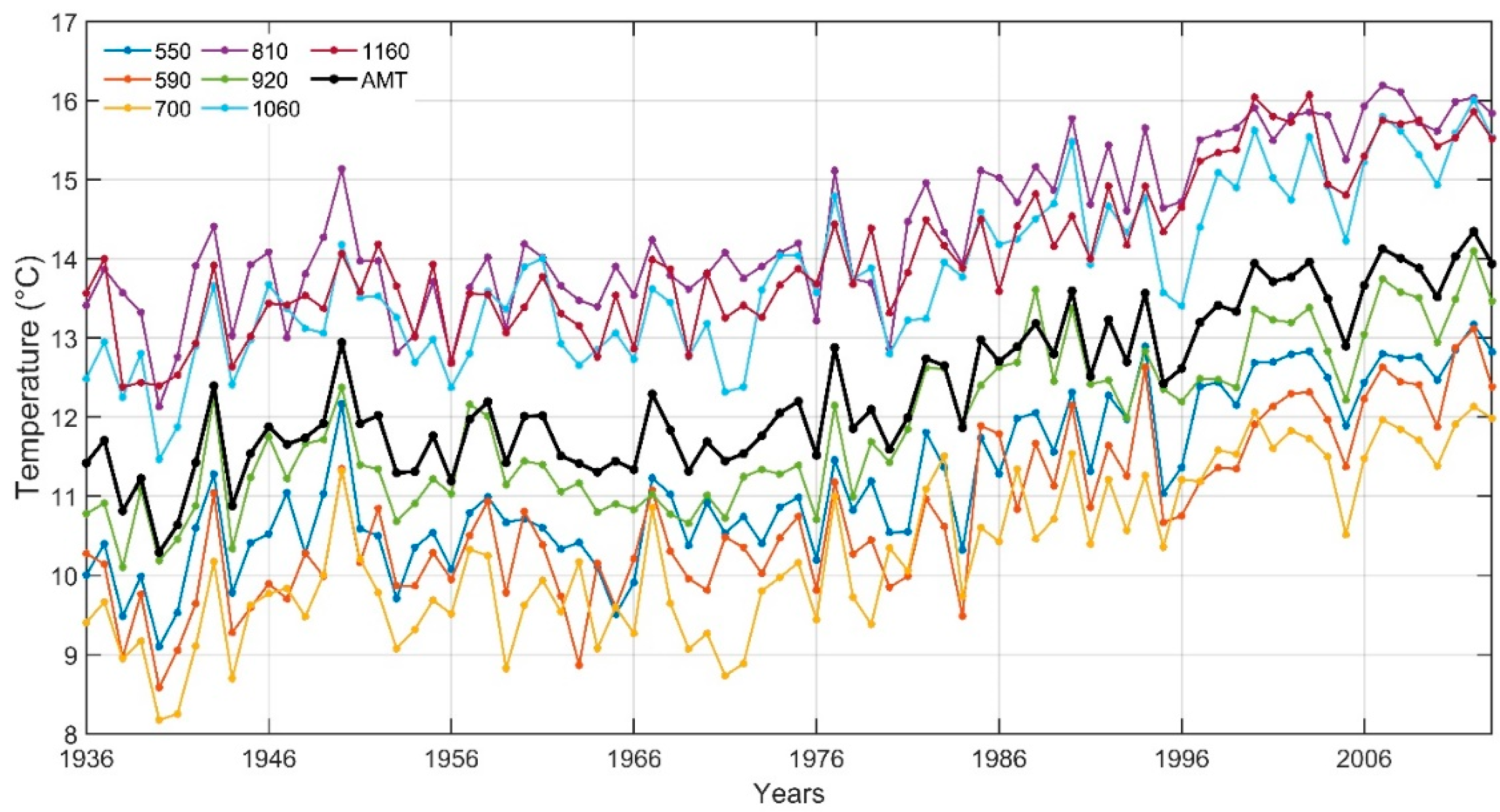
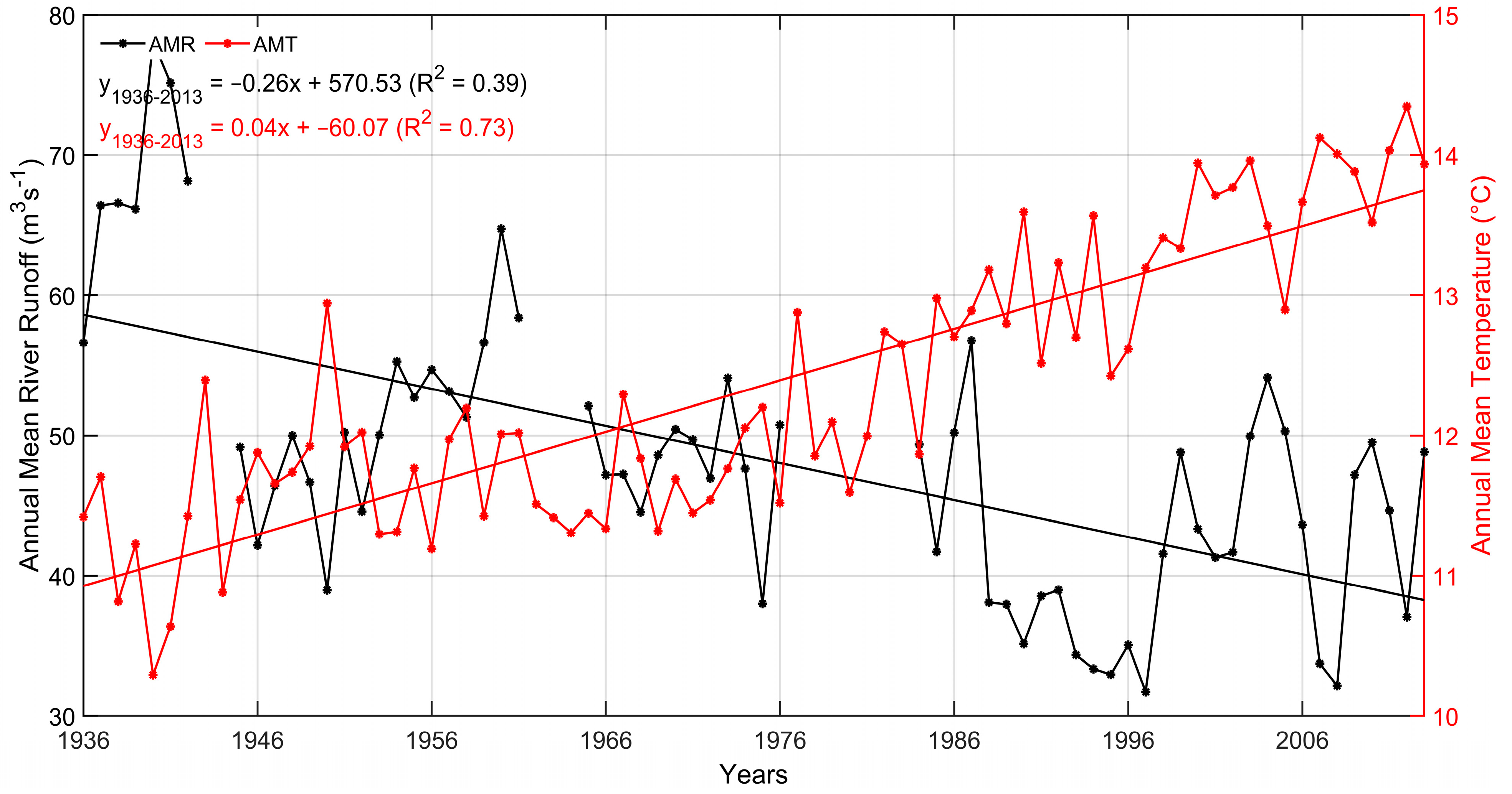
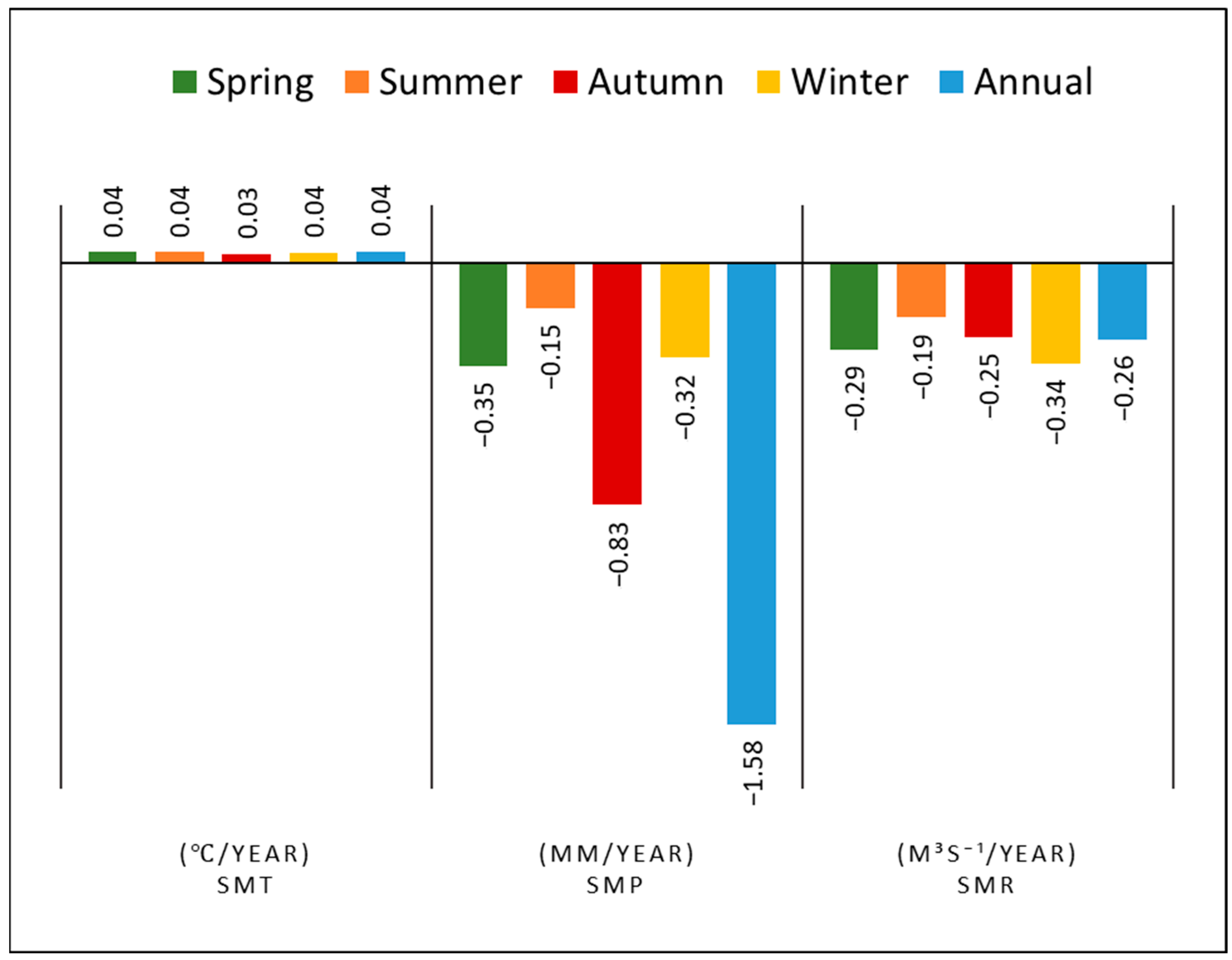
  • The annual mean temperature on the watershed scale increased at a rate of 0.037 °C/year. Spring and summer remained the hottest seasons, significantly exhibiting an increasing trend of 0.038 °C/year.
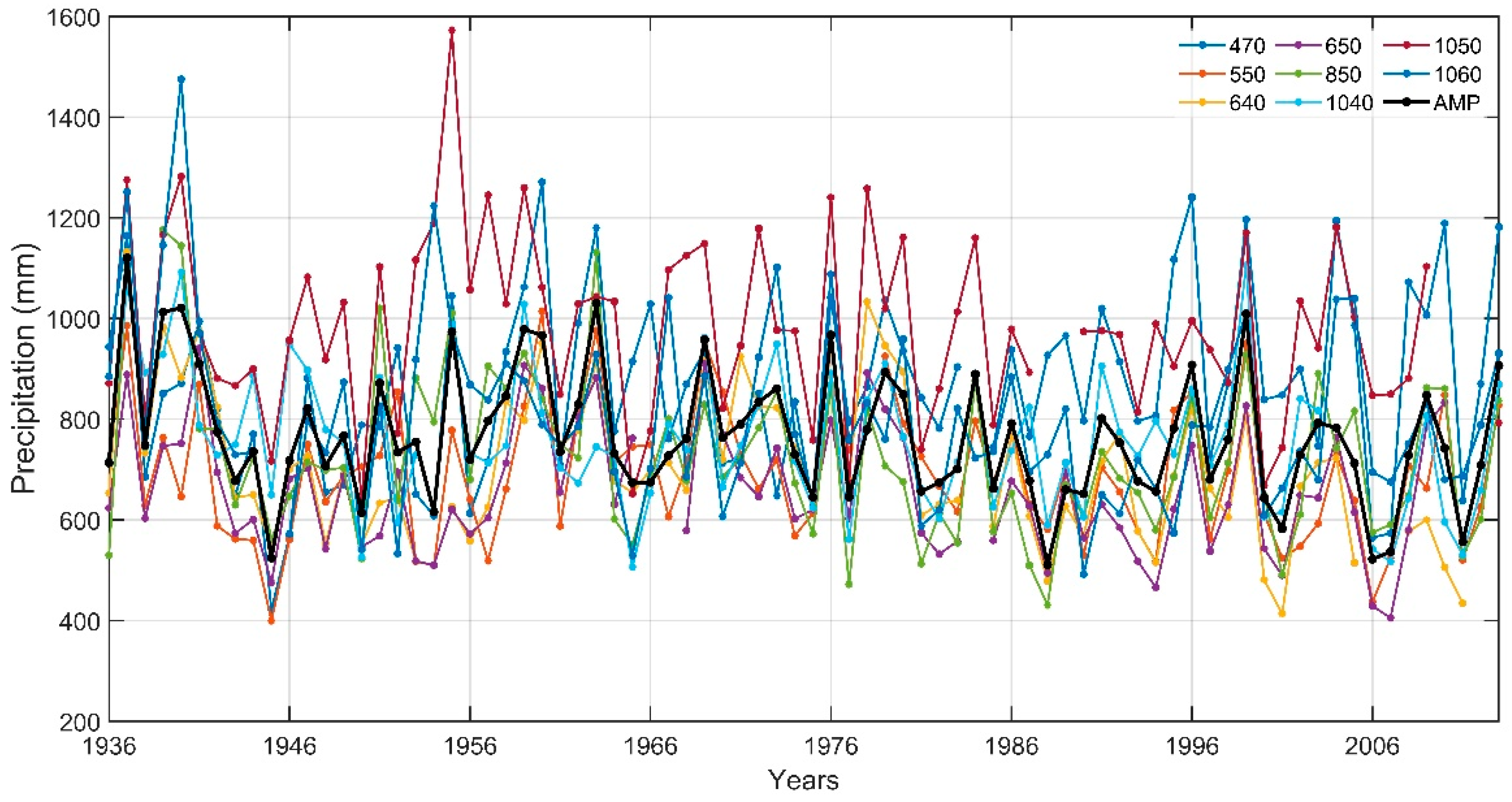
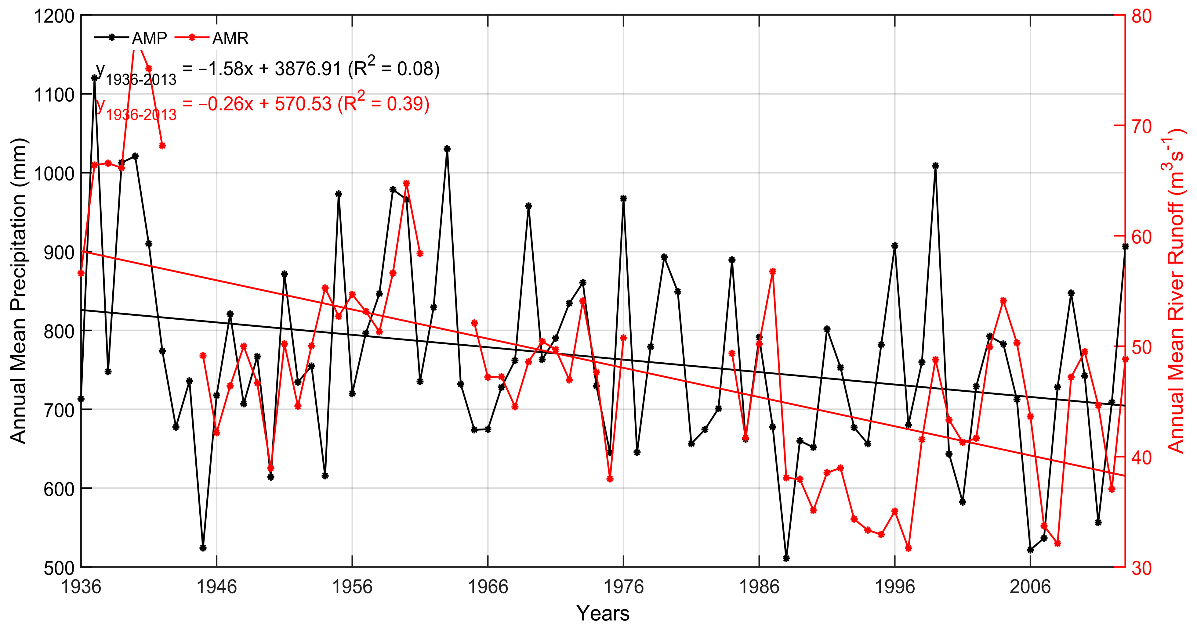
  • The cumulative precipitation average exhibited a significant decreasing trend on the annual scale and for the autumn season only. Other seasons showed an insignificant decreasing trend. The autumn season held a major contribution of −0.68 mm/year towards annual precipitation (−1.81 mm/year).
  • In association with increasing temperatures and decreasing precipitation, the hydrologic variable, i.e., RR, showed a significant decreasing trend annually (−0.29 m3 s−1/year) and seasonally, notably with the highest rate of decrease in winters (−0.41 m3 s−1/year).
  • A significant correlation was observed among all the variables, albeit with varying magnitudes of strength. To comprehensively understand their contributions towards the reduction in precipitation and RR rate, the inclusion of additional variables, such as wind matrices, water abstraction, and land use, would help.
This research could be helpful for water management agencies to consider decreasing precipitation and river runoff for future planning. Downward trends in the variables could lead to meteorological and hydrological droughts.

Author Contributions

Conceptualization and methodology, M.T., E.A. and P.D.C. Data curation, formal analysis, investigation, software, and writing—original draft, M.T. Writing—review and editing, E.A., P.C. and P.D.C. Funding acquisition, project administration, and resources, P.D.C. All authors have read and agreed to the published version of the manuscript.

Funding

Mohsin Tariq was funded with a PON fellowship under the Ricerca e Innovazione 2014–2020 program by the Ministry of University and Research. Eleonora Aruffo was supported by the European Union’s Horizon 2020 research and innovation programme under the Marie Sklodowska-Curie grant agreement (number 840217). In addition, Eleonora Aruffo, Piero Chiacchiaretta, and Piero Di Carlo received partial funding from Fondi di Ricerca Dipartimentali (Fondi ex-60% DTIMO).

Institutional Review Board Statement

Not applicable.

Informed Consent Statement

Not applicable.

Data Availability Statement

The dataset used in this study can be requested from the National Hydrographic Service (Abruzzo region).

Acknowledgments

We thank the National Hydrographic Service (Abruzzo region) for providing access to their precipitation and river runoff database.

Conflicts of Interest

All the authors who presented their mutual opinions in this study declare no conflicts of interest.

References

  1. Rahmani, F.; Fattahi, M.H. Climate change-induced influences on the nonlinear dynamic patterns of precipitation and temperatures (case study: Central England). Theor. Appl. Climatol. 2023, 152, 1147–1158. [Google Scholar] [CrossRef]
  2. Nikzad Tehrani, E.; Sahour, H.; Booij, M. Trend analysis of hydro-climatic variables in the north of Iran. Theor. Appl. Climatol. 2019, 136, 85–97. [Google Scholar] [CrossRef]
  3. Alexander, L.V.; Zhang, X.; Peterson, T.C.; Caesar, J.; Gleason, B.; Klein Tank, A.; Haylock, M.; Collins, D.; Trewin, B.; Rahimzadeh, F. Global observed changes in daily climate extremes of temperature and precipitation. J. Geophys. Res. Atmos. 2006, 111. [Google Scholar] [CrossRef]
  4. Dey, R.; Lewis, S.C.; Arblaster, J.M.; Abram, N.J. A review of past and projected changes in Australia’s rainfall. Wiley Interdiscip. Rev. Clim. Chang. 2019, 10, e577. [Google Scholar] [CrossRef]
  5. Philandras, C.; Nastos, P.; Kapsomenakis, J.; Douvis, K.; Tselioudis, G.; Zerefos, C. Long term precipitation trends and variability within the Mediterranean region. Nat. Hazards Earth Syst. Sci. 2011, 11, 3235–3250. [Google Scholar] [CrossRef]
  6. Ren, L.; Arkin, P.; Smith, T.M.; Shen, S.S. Global precipitation trends in 1900–2005 from a reconstruction and coupled model simulations. J. Geophys. Res. Atmos. 2013, 118, 1679–1689. [Google Scholar] [CrossRef]
  7. Cortesi, N.; González-Hidalgo, J.C.; Brunetti, M.; Martin-Vide, J. Daily precipitation concentration across Europe 1971–2010. Nat. Hazards Earth Syst. Sci. 2012, 12, 2799–2810. [Google Scholar] [CrossRef]
  8. Trenberth, K.E.; Jones, P.D.; Ambenje, P.; Bojariu, R.; Easterling, D.; Tank, A.K.; Parker, D.; Rahimzadeh, F.; Renwick, J.A.; Rusticucci, M. Observations: Surface and atmospheric climate change. In Climate Change 2007: The Physical Science Basis. Contribution of Working Group 1 to the 4th Assessment Report of the Intergovernmental Panel on Climate Change; Cambridge University Press: Cambridge, UK, 2007. [Google Scholar]
  9. Luterbacher, J.; Dietrich, D.; Xoplaki, E.; Grosjean, M.; Wanner, H. European seasonal and annual temperature variability, trends, and extremes since 1500. Science 2004, 303, 1499–1503. [Google Scholar] [CrossRef] [PubMed]
  10. Alpert, P.; Krichak, S.O.; Shafir, H.; Haim, D.; Osetinsky, I. Climatic trends to extremes employing regional modeling and statistical interpretation over the E. Mediterranean. Glob. Planet. Chang. 2008, 63, 163–170. [Google Scholar] [CrossRef]
  11. Tuel, A.; Eltahir, E.A. Why is the Mediterranean a climate change hot spot? J. Clim. 2020, 33, 5829–5843. [Google Scholar] [CrossRef]
  12. Climate Change 2022: Impacts, Adaptation, and Vulnerability. Contribution of Working Group II to the Sixth Assessment Report of the Intergovernmental Panel on Climate Change; IPCC: Geneva, Switzerland, 2022.
  13. Jackson, R.B.; Carpenter, S.R.; Dahm, C.N.; McKnight, D.M.; Naiman, R.J.; Postel, S.L.; Running, S.W. Water in a changing world. Ecol. Appl. 2001, 11, 1027–1045. [Google Scholar] [CrossRef]
  14. Gudmundsson, L.; Boulange, J.; Do, H.X.; Gosling, S.N.; Grillakis, M.G.; Koutroulis, A.G.; Leonard, M.; Liu, J.; Müller Schmied, H.; Papadimitriou, L. Globally observed trends in mean and extreme river flow attributed to climate change. Science 2021, 371, 1159–1162. [Google Scholar] [CrossRef] [PubMed]
  15. Donnelly, C.; Greuell, W.; Andersson, J.; Gerten, D.; Pisacane, G.; Roudier, P.; Ludwig, F. Impacts of climate change on European hydrology at 1.5, 2 and 3 degrees mean global warming above preindustrial level. Clim. Chang. 2017, 143, 13–26. [Google Scholar] [CrossRef]
  16. Noto, L.V.; Cipolla, G.; Francipane, A.; Pumo, D. Climate change in the mediterranean basin (part I): Induced alterations on climate forcings and hydrological processes. Water Resour. Manag. 2023, 37, 2287–2305. [Google Scholar] [CrossRef]
  17. Vicente-Serrano, S.M.; Peña-Gallardo, M.; Hannaford, J.; Murphy, C.; Lorenzo-Lacruz, J.; Dominguez-Castro, F.; López-Moreno, J.I.; Beguería, S.; Noguera, I.; Harrigan, S. Climate, irrigation, and land cover change explain streamflow trends in countries bordering the northeast Atlantic. Geophys. Res. Lett. 2019, 46, 10821–10833. [Google Scholar] [CrossRef]
  18. Hao, X.; Chen, Y.; Xu, C.; Li, W. Impacts of climate change and human activities on the surface runoff in the Tarim River Basin over the last fifty years. Water Resour. Manag. 2008, 22, 1159–1171. [Google Scholar] [CrossRef]
  19. Gudmundsson, L.; Seneviratne, S.I.; Zhang, X. Anthropogenic climate change detected in European renewable freshwater resources. Nat. Clim. Chang. 2017, 7, 813–816. [Google Scholar] [CrossRef]
  20. Brunetti, M.; Maugeri, M.; Nanni, T. Variations of temperature and precipitation in Italy from 1866 to 1995. Theor. Appl. Climatol. 2000, 65, 165–174. [Google Scholar] [CrossRef]
  21. Caloiero, T.; Coscarelli, R.; Ferrari, E.; Mancini, M. Trend detection of annual and seasonal rainfall in Calabria (Southern Italy). Int. J. Climatol. 2011, 31, 44–56. [Google Scholar] [CrossRef]
  22. Vergni, L.; Todisco, F. Spatio-temporal variability of precipitation, temperature and agricultural drought indices in Central Italy. Agric. For. Meteorol. 2011, 151, 301–313. [Google Scholar] [CrossRef]
  23. Toreti, A.; Desiato, F. Temperature trend over Italy from 1961 to 2004. Theor. Appl. Climatol. 2008, 91, 51–58. [Google Scholar] [CrossRef]
  24. Gentilucci, M.; Materazzi, M.; Pambianchi, G.; Burt, P.; Guerriero, G. Assessment of variations in the temperature-rainfall trend in the province of Macerata (Central Italy), comparing the last three climatological standard normals (1961–1990; 1971–2000; 1981–2010) for biosustainability studies. Environ. Process. 2019, 6, 391–412. [Google Scholar] [CrossRef]
  25. Aruffo, E.; Di Carlo, P. Homogenization of instrumental time series of air temperature in Central Italy (1930–2015). Clim. Res. 2019, 77, 193–204. [Google Scholar] [CrossRef]
  26. Scorzini, A.R.; Leopardi, M. Precipitation and temperature trends over central Italy (Abruzzo Region): 1951–2012. Theor. Appl. Climatol. 2019, 135, 959–977. [Google Scholar] [CrossRef]
  27. Curci, G.; Guijarro, J.A.; Di Antonio, L.; Di Bacco, M.; Di Lena, B.; Scorzini, A.R. Building a local climate reference dataset: Application to the Abruzzo region (Central Italy), 1930–2019. Int. J. Climatol. 2021, 41, 4414–4436. [Google Scholar] [CrossRef]
  28. Farroni, A.; Magaldi, D.; Tallini, M. Total sediment transport by the rivers of Abruzzi (Central Italy): Prediction with the Raizal model. Bull. Eng. Geol. Environ. 2002, 61, 121–127. [Google Scholar]
  29. Lastoria, B.; Miserocchi, F.; Lanciani, A.; Monacelli, G. An estimated erosion map for the Aterno-Pescara river basin. Eur. Water 2008, 21, 29–39. [Google Scholar]
  30. Tariq, M.; Rohith, A.; Cibin, R.; Aruffo, E.; Abouzied, G.A.A.; Di Carlo, P. Understanding future hydrologic challenges: Modelling the impact of climate change on river runoff in central Italy. Environ. Chall. 2024, 15, 100899. [Google Scholar] [CrossRef]
  31. WMO. Analyzing Long Time Series of Hydrological Data with Respect to Climate Variability; World Meteorological Organization: Geneva, Switzerland, 1988. [Google Scholar]
  32. Darvini, G.; Memmola, F. Assessment of the impact of climate variability and human activities on the runoff in five catchments of the Adriatic Coast of south-central Italy. J. Hydrol. Reg. Stud. 2020, 31, 100712. [Google Scholar] [CrossRef]
  33. Anghileri, D.; Pianosi, F.; Soncini-Sessa, R. Trend detection in seasonal data: From hydrology to water resources. J. Hydrol. 2014, 511, 171–179. [Google Scholar] [CrossRef]
  34. Mann, H.B. Nonparametric tests against trend. Econometrica 1945, 13, 245–259. [Google Scholar] [CrossRef]
  35. Kendall, M.G. Rank Correlation Methods; American Psychological Association: Washington, DC, USA, 1948. [Google Scholar]
  36. Aalijahan, M.; Karataş, A.; Lupo, A.R.; Efe, B.; Khosravichenar, A. Analyzing and modeling the spatial-temporal changes and the impact of GLOTI index on precipitation in the Marmara region of Türkiye. Atmosphere 2023, 14, 489. [Google Scholar] [CrossRef]
  37. Camuffo, D.; Bertolin, C.; Diodato, N.; Cocheo, C.; Barriendos, M.; Dominguez-Castro, F.; Garnier, E.; Alcoforado, M.J.; Nunes, M. Western Mediterranean precipitation over the last 300 years from instrumental observations. Clim. Chang. 2013, 117, 85–101. [Google Scholar] [CrossRef]
  38. Yue, S.; Wang, C.Y. Applicability of prewhitening to eliminate the influence of serial correlation on the Mann-Kendall test. Water Resour. Res. 2002, 38, 4-1–4-7. [Google Scholar] [CrossRef]
  39. Yue, S.; Wang, C. The Mann-Kendall test modified by effective sample size to detect trend in serially correlated hydrological series. Water Resour. Manag. 2004, 18, 201–218. [Google Scholar] [CrossRef]
  40. Sandeep Kumar, P.; Nicole, O.B. Modifiedmk: Modified Versions of Mann Kendall and Spearman’s Rho Trend Tests. 2021, R Package Version 1.6. Available online: https://CRAN.R-project.org/package=modifiedmk (accessed on 10 November 2023).
  41. Wang, W.; Yin, S.; Gao, G.; Papalexiou, S.; Wang, Z. Increasing trends in rainfall erosivity in the Yellow River basin from 1971 to 2020. J. Hydrol. 2022, 610, 127851. [Google Scholar] [CrossRef]
  42. Sen, P.K. Estimates of the regression coefficient based on Kendall’s tau. J. Am. Stat. Assoc. 1968, 63, 1379–1389. [Google Scholar]
  43. Yue, S.; Pilon, P.; Cavadias, G. Power of the Mann–Kendall and Spearman’s rho tests for detecting monotonic trends in hydrological series. J. Hydrol. 2002, 259, 254–271. [Google Scholar] [CrossRef]
  44. Klein Tank, A.M.G.; Wijngaard, J.B.; Können, G.P.; Böhm, R.; Demarée, G.; Gocheva, A.; Mileta, M.; Pashiardis, S.; Hejkrlik, L.; Kern-Hansen, C.; et al. Daily dataset of 20th-century surface air temperature and precipitation series for the European Climate Assessment. Int. J. Climatol. 2002, 22, 1441–1453. [Google Scholar] [CrossRef]
  45. Ventura, F.; Pisa, P.R.; Ardizzoni, E. Temperature and precipitation trends in Bologna (Italy) from 1952 to 1999. Atmos. Res. 2002, 61, 203–214. [Google Scholar] [CrossRef]
  46. Kumar, P.V.; Bindi, M.; Crisci, A.; Maracchi, G. Detection of variations in air temperature at different time scales during the period 1889–1998 at Firenze, Italy. Clim. Chang. 2005, 72, 123–150. [Google Scholar] [CrossRef]
  47. Bartolini, G.; Morabito, M.; Crisci, A.; Grifoni, D.; Torrigiani, T.; Petralli, M.; Maracchi, G.; Orlandini, S. Recent trends in Tuscany (Italy) summer temperature and indices of extremes. Int. J. Climatol. 2008, 28, 1751–1760. [Google Scholar] [CrossRef]
  48. Viola, F.; Liuzzo, L.; Noto, L.V.; Lo Conti, F.; La Loggia, G. Spatial distribution of temperature trends in Sicily. Int. J. Climatol. 2014, 34, 1–17. [Google Scholar] [CrossRef]
  49. Moonen, A.C.; Ercoli, L.; Mariotti, M.; Masoni, A. Climate change in Italy indicated by agrometeorological indices over 122 years. Agric. For. Meteorol. 2002, 111, 13–27. [Google Scholar] [CrossRef]
  50. Longobardi, A.; Buttafuoco, G.; Caloiero, T.; Coscarelli, R. Spatial and temporal distribution of precipitation in a Mediterranean area (southern Italy). Environ. Earth Sci. 2016, 75, 1–20. [Google Scholar] [CrossRef]
  51. Caporali, E.; Lompi, M.; Pacetti, T.; Chiarello, V.; Fatichi, S. A review of studies on observed precipitation trends in Italy. Int. J. Climatol. 2021, 41, E1–E25. [Google Scholar] [CrossRef]
  52. Kubiak-Wójcicka, K.; Nagy, P.; Pilarska, A.; Zeleňáková, M. Trend analysis of selected hydroclimatic variables for the Hornad catchment (Slovakia). Water 2023, 15, 471. [Google Scholar] [CrossRef]
  53. López-Moreno, J.; Vicente-Serrano, S.; Morán-Tejeda, E.; Lorenzo-Lacruz, J.; Kenawy, A.; Beniston, M. Effects of the North Atlantic Oscillation (NAO) on combined temperature and precipitation winter modes in the Mediterranean mountains: Observed relationships and projections for the 21st century. Glob. Planet. Chang. 2011, 77, 62–76. [Google Scholar] [CrossRef]
  54. Fernández, J.; Sáenz, J.; Zorita, E. Analysis of wintertime atmospheric moisture transport and its variability over southern Europe in the NCEP Reanalyses. Clim. Res. 2003, 23, 195–215. [Google Scholar] [CrossRef]
  55. Quadrelli, R.; Pavan, V.; Molteni, F. Wintertime variability of Mediterranean precipitation and its links with large-scale circulation anomalies. Clim. Dyn. 2001, 17, 457–466. [Google Scholar] [CrossRef]
  56. Memmola, F.; Darvini, G. Changes in Precipitation-Runoff Relationship in Six Catchments of the Adriatic Coast of Central Italy. EPiC Ser. Eng. 2018, 3, 1373–1381. [Google Scholar]
  57. Saidi, H.; Dresti, C.; Manca, D.; Ciampittiello, M. Quantifying impacts of climate variability and human activities on the streamflow of an Alpine river. Environ. Earth Sci. 2018, 77, 1–16. [Google Scholar] [CrossRef]
  58. Gentilucci, M.; Djouohou, S.I.; Barbieri, M.; Hamed, Y.; Pambianchi, G. Trend Analysis of Streamflows in Relation to Precipitation: A Case Study in Central Italy. Water 2023, 15, 1586. [Google Scholar] [CrossRef]
Figure 1. The map shows the Aterno-Pescara River watershed, the location of installed measuring stations, and other rivers in the Abruzzo region, adapted from [30].
Sustainability 17 00493 g001
Figure 2. Station-wise annual mean temperatures (1936–2013) show variations among various stations. The legend reports the station code; see Table 2 and Figure 1 for the location.
Sustainability 17 00493 g002
Figure 3. Station-wise total annual precipitation (1936–2013) shows variations among various stations. The legend reports the same information as Figure 2.
Sustainability 17 00493 g003
Figure 4. The linear regression comparison plot of AMP and AMT (1936–2013) shows an increase in AMT and a decrease in AMP.
Sustainability 17 00493 g004
Figure 5. The linear regression comparison plot of AMR and AMT (1936–2013) shows a decrease in AMR and an increase in AMT.
Sustainability 17 00493 g005
Figure 6. The linear regression comparison plot of AMP and AMR (1936–2013) shows a decrease in AMR and AMP.
Sustainability 17 00493 g006
Figure 7. The linear regression comparison plot of SMP and SMT (1936–2013) shows an increase in SMT and a decrease in SMP.
Sustainability 17 00493 g007
Figure 8. The linear regression comparison plot of SMR and SMT (1936–2013) shows a decrease in SMR and an increase in SMT.
Sustainability 17 00493 g008
Figure 9. The linear regression comparison plot of SMP and SMR (1936–2013) shows decreases in SMP and SMR.
Sustainability 17 00493 g009
Figure 10. Comparison of SMT, SMP, and SMR with annual linear slopes. SMT indicates an increase, and SMP and SMR show a decrease in seasons and on an annual scale.
Sustainability 17 00493 g010
Table 1. Tributaries of the Aterno-Pescara River.
River Basin Area (km2) Area Percentage to the Total Watershed (%)
Raio River260.368.21
Sagittario River612.9019.33
Gizio River253.508.05
Orta River165.565.22
Vera River137.894.35
Tirino River369.4711.73
Nora River137.664.34
Table 2. List of stations measuring precipitation (Pcp), temperature (Tmp), and river runoff (Hydro).
Station Name Type Elevation (m) Above Sea Level NHS Code
MonterealePcp913.00470
L’Aquila a S. EliaPcp595.00550
BeffiPcp608.00640
CampanaPcp563.00650
PopoliPcp250.00850
AlannoPcp285.001040
ManoppelloPcp297.001050
ChietiPcp278.001060
L’Aquila a S. EliaTmp595.00550
AssergiTmp992.00590
ScannoTmp1045.00700
SulmonaTmp372.00810
BariscianoTmp978.00920
ChietiTmp278.001060
PescaraTmp2.001160
Pescara a Santa TeresaHydro4.506140
Table 3. Summary statistics of measured cumulative daily temperatures (°C).
Months 1936–2013
TminTmaxTdaySTDTdaySkKrCv (%)
January0.406.933.661.700.190.5446.51
February0.738.174.451.700.190.5338.08
March3.1611.397.271.680.151.1323.06
April6.1415.0410.591.720.181.2716.26
May10.0719.7814.921.730.221.3011.60
June13.5224.1518.831.840.151.229.78
July15.8427.5121.671.710.161.377.88
August15.9227.5621.741.640.071.517.55
September12.9423.1618.051.710.050.979.45
October9.1117.6513.381.750.110.7513.04
November5.1212.138.621.820.230.6121.13
December1.767.934.851.870.210.7838.54
Table 4. Summary statistics of cumulative precipitation (mm) and river runoff (m3 s−1).
Months 1936–2013 1936–2013
PCPSTDSkKrCv (%)RRSTDSkKrCv (%)
January70.9412.201.315.1717.2055.0414.910.823.7327.09
February63.347.671.404.2412.1157.1415.500.502.9127.12
March61.6810.961.245.1617.7858.2015.210.252.4526.13
April67.3412.460.613.1118.5158.7716.810.803.3028.60
May57.158.101.252.7914.1748.9413.341.033.5527.26
June47.617.17−0.071.0215.0741.2011.601.586.7228.15
July34.704.90−0.772.1914.1235.887.681.336.8921.40
August39.208.130.141.3820.7334.927.76−0.718.7222.23
September61.7710.350.061.2816.7539.438.110.913.9120.57
October78.9111.921.084.7715.1143.5110.441.456.9824.00
November97.679.550.962.539.7849.9412.750.753.3625.54
December92.5913.121.324.7514.1755.9015.661.235.8028.01
Table 5. MK and SSE test results.
Time Period MK Test SSE Test
TMPPCPRRTMPPCPRR
ZSig.ZSig.ZSig.bsenbsenbsen
1936–20136.15**−2.47*−2.29*0.037−1.81−0.29
Spring6.06**−1.34+−2.72**0.038−0.42−0.35
Summer5.56**−0.6+−2.35*0.038−0.16−0.18
Autumn5.52**−2.55*−3.52**0.031−0.68−0.28
Winter5.82**−1.20+−3.21**0.034−0.38−0.41
“+” indicates an insignificant trend, while “*” and “**” represent significant trends at the 95% and 99% confidence levels, respectively.
Table 6. Spearman correlation coefficients between hydro-climatic variables.
Time Period TMP vs. PCP TMP vs. RR PCP vs. RR
rsSig.rsSig.rsSig.
1936–2013−0.40**−0.62**0.46**
Spring−0.31**−0.56**0.47**
Summer−0.42**−0.53*0.21**
Autumn−0.28*−0.45**0.40**
Winter−0.29**−0.61**0.52**
“*” and “**” represent significant trends at the 95% and 99% confidence levels, respectively.
Disclaimer/Publisher’s Note: The statements, opinions and data contained in all publications are solely those of the individual author(s) and contributor(s) and not of MDPI and/or the editor(s). MDPI and/or the editor(s) disclaim responsibility for any injury to people or property resulting from any ideas, methods, instructions or products referred to in the content.

