Article

Short-Term Passenger Flow Forecasting for Rail Transit Inte-Grating Multi-Scale Decomposition and Deep Attention Mechanism

School of Mathematics and Physics, Lanzhou Jiaotong University, Lanzhou 730070, China
*
Author to whom correspondence should be addressed.
Sustainability 2025, 17(19), 8880; https://doi.org/10.3390/su17198880
Submission received: 7 September 2025 / Revised: 1 October 2025 / Accepted: 3 October 2025 / Published: 6 October 2025

Abstract

Short-term passenger flow prediction provides critical data-driven support for optimizing resource allocation, guiding passenger mobility, and enhancing risk response capabilities in urban rail transit systems. To further improve prediction accuracy, this study proposes a hybrid SMA-VMD-Informer-BiLSTM prediction model. Addressing the challenge of error propagation caused by non-stationary components (e.g., noise and abrupt fluctuations) in conventional passenger flow signals, the Variational Mode Decomposition (VMD) method is introduced to decompose raw flow data into multiple intrinsic mode functions (IMFs). A Slime Mould Algorithm (SMA)-based optimization mechanism is designed to adaptively tune VMD parameters, effectively mitigating mode redundancy and information loss. Furthermore, to circumvent error accumulation inherent in serial modeling frameworks, a parallel prediction architecture is developed: the Informer branch captures long-term dependencies through its ProbSparse self-attention mechanism, while the Bidirectional Long Short-Term Memory (BiLSTM) network extracts localized short-term temporal patterns. The outputs of both branches are fused via a fully connected layer, balancing global trend adherence and local fluctuation characterization. Experimental validation using historical entry flow data from Weihouzhuang Station on Xi’an Metro demonstrated the superior performance of the SMA-VMD-Informer-BiLSTM model. Compared to benchmark models (CNN-BiLSTM, CNN-BiGRU, Transformer-LSTM, ARIMA-LSTM), the proposed model achieved reductions of 7.14–53.33% in f m s e , 3.81–31.14% in f r m s e , and 8.87–38.08% in f m a e , alongside a 4.11–5.48% improvement in R 2 . Cross-station validation across multiple Xi’an Metro hubs further confirmed robust spatial generalizability, with prediction errors bounded within f m s e : 0.0009–0.01, f r m s e : 0.0303–0.1, f m a e : 0.0196–0.0697, and R 2 : 0.9011–0.9971. Furthermore, the model demonstrated favorable predictive performance when applied to forecasting passenger inflows at multiple stations in Nanjing and Zhengzhou, showcasing its excellent spatial transferability. By integrating multi-level, multi-scale data processing and adaptive feature extraction mechanisms, the proposed model significantly mitigates error accumulation observed in traditional approaches. These findings collectively indicate its potential as a scientific foundation for refined operational decision-making in urban rail transit management, thereby significantly promoting the sustainable development and long-term stable operation of urban rail transit systems.

1. Introduction

From an international perspective, during the period from 2010 to 2021, Europe’s railway transport exhibited a steady and systematic growth trend [1]. Focusing on China, By the end of 2024, a total of 54 cities in China had opened urban rail transit lines, with the total operational mileage of metro lines reaching 10,945.6 km. Throughout the year 2024, China’s urban rail transit system handled 32.24 billion passenger trips, marking an increase of 2.8 billion passenger trips or a 9.5% growth compared to 2023. Furthermore, as the urban rail transit network continues to improve, passenger volume on urban rail transit is still on the rise. Intelligent Transportation Systems (ITSs) have emerged as a pivotal transformative force in advancing the achievement of the United Nations Sustainable Development Goals (SDGs) [2], increasingly underscoring their strategic significance. Among its enabling technologies, short-term passenger flow prediction stands out by accurately capturing real-time dynamic patterns in passenger demand. This capability not only provides rail transit operators with a scientific basis for optimized resource allocation and dynamic, intelligent adjustment of train operation plans but also facilitates the establishment of rapid response mechanisms during emergency scenarios such as sudden passenger surges. Consequently, it serves as a cornerstone technology for comprehensively elevating both the service quality and operational resilience of urban rail transit systems.
Machine learning models represent the mainstream approach for short-term passenger flow forecasting in urban rail transit. Initially, models such as Random Forest [3], Multilayer Perceptron [4], and Support Vector Machine (SVM) [5,6] were employed. Subsequently, some studies integrated methods like Autoregressive Integrated Moving Average Model (ARIMA) with Support Vector Machine [7], ARIMA with Wavelet Neural Network [8], and ARIMA with Back Propagation Neural Networks (BPNNs) [9,10], forming hybrid forecasting models that demonstrated relatively high prediction accuracy. However, these machine learning models typically require manual feature extraction and exhibit limited capability in handling complex and high-dimensional data.
Currently, deep learning has taken a dominant position, owing to its powerful representational capabilities and automatic feature extraction abilities, which enable it to swiftly process high-dimensional and complex data, thereby more accurately reflecting the changing trends in passenger flow. Ma et al. [11] first employed Long Short-Term Memory (LSTM) for forecasting in 2015, while Zhang Huizhen et al. [12] utilized LSTM and Gated Recurrent Unit (GRU) separately to predict passenger flow at different types of stations during various time periods. Given the limitations of single models, ensemble models further enhance prediction accuracy and robustness by integrating the strengths of different models. Liu et al. [13] proposed an LSTM-Fully Connected (LSTM-FC) ensemble model, combining LSTM’s sequence modeling capability with the feature integration ability of the FC layer, effectively capturing both long-term and short-term dependencies in the data while efficiently integrating and reducing the dimensionality of the extracted high-dimensional features. Zeng Lu et al. [14] introduced a Complete Ensemble Empirical Mode Decomposition with Adaptive Noise-Improved Particle Swarm Optimization-LSTM (CEEMDAN-IPSO-LSTM) ensemble model, significantly improving the prediction accuracy and robustness of LSTM through multi-scale feature extraction and hyperparameter optimization. Li et al. [15] proposed a Convolutional Neural Network-Residual Network-Bidirectional Long Short-Term Memory (CNN-ResNet-BiLSTM) model, further enhancing prediction accuracy and noise resistance through multi-level feature fusion and deep residual networks. Other researchers, such as Gao [16], Wang [17], and Wang et al. [18], have also proposed ensemble models with different architectures and validated their effectiveness.
Li et al. [19] proposed a residual neural network for predicting the entire Origin-Destination (O-D) flow and demonstrated the robustness of this framework. Wang et al. [20] introduced a deep learning (DL)-based Stacked Sparse Autoencoder (SAE) model for accurately estimating network traffic from flow data, thereby enhancing efficiency. A comparative overview of relevant studies is presented in Table 1.
In summary, significant progress has been made in existing research; however, there remain deficiencies in aspects such as data processing, model selection, and parameter optimization. Firstly, inadequate handling of non-stationary components such as noise and abrupt changes leads to error accumulation in prediction models, thereby resulting in a decline in prediction accuracy. Secondly, insufficient capture of both long-term and short-term dependencies is observed, as some serial ensemble models tend to emphasize one type of dependency over the other, causing errors to accumulate in the same direction and ultimately leading to biased prediction outcomes. In light of these issues, this paper constructs a novel deep learning ensemble model, namely SMA-VMD-Informer-BiLSTM, which incorporates Variational Mode Decomposition (VMD) and Slime Mould Algorithm (SMA) for modal decomposition and parameter optimization, respectively. Subsequently, it designs a parallel prediction framework integrating Informer and Bidirectional Long Short-Term Memory (BiLSTM) networks to simultaneously capture long-term and short-term dependencies, thereby addressing the aforementioned shortcomings. Furthermore, the accuracy and portability of the model are validated using passenger flow data from Xi’an urban rail transit. The primary contributions of this paper are outlined as follows:
(1)
Data Layer Optimization: Enhancing Input Signal Quality
On one hand, the original passenger flow signals are decomposed into stable signals of different frequencies through VMD, thereby avoiding the modal aliasing issue that is prone to occur in traditional methods. On the other hand, the SMA is introduced to dynamically optimize the parameters of VMD, circumventing the problems of modal omission or modal redundancy that are likely to arise from manual parameter setting.
(2)
Model Layer Innovation: Improving Prediction Model Architecture
On one hand, the Informer branch is leveraged to efficiently capture long-term patterns such as morning and evening peak hours, while the BiLSTM branch is employed to efficiently capture short-term patterns. On the other hand, the outputs of the two branches are concatenated and then passed through a fully connected layer to achieve feature interaction and generate the final output, thereby enabling accurate prediction of short-term passenger entry flows.
The structural arrangement of this paper is as follows: Section 2 introduces the construction of relevant models; Section 3 presents a case study.; Section 4 presents the conclusions.

2. Methods

2.1. Denoising Decomposition Method Based on SMA-VMD

The SMA proposed by Li et al. [21] in 2020, is an optimization algorithm inspired by the behavior of natural slime moulds. When searching for food and adapting to their environment, slime moulds exhibit a high degree of adaptability and flexibility, making them a suitable basis for solving optimization problems. VMD [22] is a signal processing technique designed to decompose complex non-stationary signals into a set of modes with distinct spectral components. Its detailed mathematical formulation is presented in Equation (1).
u , u ^ , ω = VMD ( f , α , τ , K , D C , i n i t , t o l )
Among the notations, the items following the equal sign represent input parameters. Here, f is the original time-domain signal to be decomposed, namely the passenger entry flow data signal. α is the bandwidth constraint parameter, τ is the noise tolerance parameter, K is the number of modal functions obtained from decomposition, D C is the retention parameter for the direct current component, i n i t denotes the initialization method, and t o l represents the convergence tolerance. The items preceding the equal sign are output parameters, where u represents the decomposed modal functions, u ^ represents the decomposed modal spectra, and ω represents the central frequencies of the decomposed modes.
To achieve more precise signal decomposition, this paper utilizes the SMA for the automatic optimization of the parameters K and α in VMD, aiming to enhance the signal reconstruction quality and processing efficiency. The optimization flowchart is depicted in Figure 1, and the detailed decomposition steps are presented as follows.
Step 1: Define parameters and initialize
Define the size of the population P , the maximum number of iterations, the upper and lower bounds of the parameters, as well as the dimensionality of the parameters. Randomly generate a set of individual positions within the parameter ranges. Each individual corresponds to a set of candidate solutions, where K is an integer and α is a real number. Then, calculate their fitness values.
Step 2: Define the fitness function
Randomly select a set of values for K and α , and perform VMD to obtain several modes u i . Then, utilize these output modes to reconstruct the signal. The reconstructed signal is denoted as f = i = 1 K u i , and the reconstruction error is r = f f 2 f 2 . We employ the reconstruction error as the fitness evaluation metric, where a smaller value indicates that the selected parameters can better reconstruct the signal.
Step 3: Iterative optimization
Traverse each individual and update the current optimal solution. In each iteration, calculate its fitness value r . If r is smaller than the fitness value of the previous iteration, update the population positions and record the current optimal fitness value along with its corresponding parameters. The position update of individuals adopts the core logic of slime mold: p i + = Δ × ( p i μ ) , where μ is the mean of the current population, and Δ represents the position change determined by a random number.
Step 4: Result visualization
Print the optimal values of K and α , and visualize the original data signal, the reconstructed signal, and the decomposed modes.

2.2. Informer-BiLSTM Model

2.2.1. Informer

Informer is an improved model [23] based on the Transformer architecture, which is better suited for processing time-series data. When addressing complex nonlinear interdependencies between time steps and variables in short-term passenger flow prediction, Informer’s generative structure effectively avoids error accumulation in multi-step predictions, demonstrating its unique advantages.
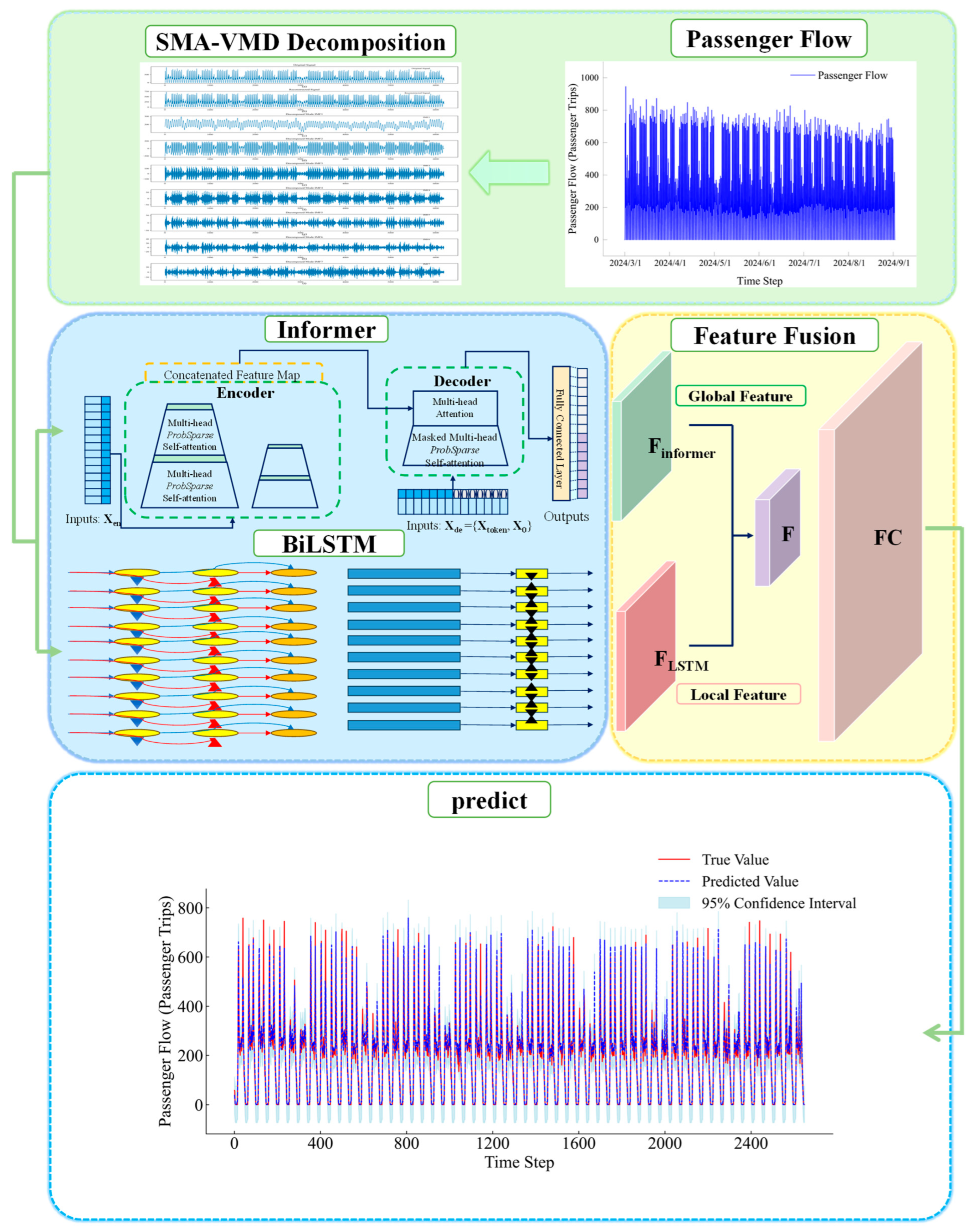
The Informer architecture primarily consists of an encoder and a decoder, with its structure illustrated in the Informer section of Figure 2. In the encoder layer, it comprises a probabilistic sparse self-attention layer and a distillation layer. The input, denoted as X e n , consists of various Intrinsic Mode Functions (IMFs) obtained from the decomposition of raw passenger flow data via SMA-VMD (Sparrow Search Algorithm-optimized Variational Mode Decomposition). These IMFs retain the key spatiotemporal features of the input sequence for utilization by the decoder. The decoder section incorporates a hidden multi-head probabilistic sparse self-attention module and a multi-head attention module. It receives the key spatiotemporal feature information from the encoder. The input, denoted as X d e , is implemented using a partially known and partially unknown strategy, i.e., the known values at the end of the IMF data sequence and zero-padding for the prediction units. Finally, the entire predicted sequence is generated in one pass through a fully connected layer, as depicted by the purple unit in the Informer structure in Figure 2.
Informer primarily introduces a probabilistic sparse self-attention mechanism and a distillation mechanism. The computational formula for its probabilistic sparse self-attention mechanism is shown in Equation (2).
A ( Q , K , V ) = S o f t max Q ¯ K d V
where A ( Q , K , V ) denotes the probabilistic sparse self-attention mechanism, with Q , K , V representing input feature matrices. K is the transpose of matrix K , Q ¯ is the probabilistic sparse matrix derived from Q via sparsification, d represents the input dimension, and S o f t max denotes the activation function.
Self-attention distillation can assign higher priority to dominant features, with its computational method shown in Equation (3).
X j + 1 t = MaxPool ELU Conv 1 d X j t AB
where MaxPool denotes the max-pooling operation, ELU represents the Exponential Linear Unit activation function, · AB signifies the multi-head sparse self-attention module combined with basic operations, and Conv 1 d refers to the 1D convolution operation applied to sequences.

2.2.2. BiLSTM

The BiLSTM network is composed of a forward LSTM and a backward LSTM, with its structure depicted in the BiLSTM section of Figure 2. By incorporating a bidirectional architecture into the network, BiLSTM captures both past and future information of the input sequence through the forward LSTM layer and the backward LSTM layer, respectively. Specifically, the forward LSTM layer and the backward LSTM layer generate two hidden layer states with opposite temporal sequences. These two hidden layer states are then combined to produce the output of the BiLSTM. The computational methods for this process are given by Equations (4)–(6).
h t ( 1 ) = LSTM x t , h t 1 ( 1 )
h t ( 2 ) = LSTM x t , h t 1 ( 2 )
y t = μ 1 h t ( 1 ) + μ 2 h t ( 2 ) + b y
In the BiLSTM model, the input layer is denoted as x t , the output layer as y t , the forward hidden layer as h t ( 1 ) , and the backward hidden layer as h t ( 2 ) . Here, μ 1 and μ 2 represent the weight matrices for the output layer, while b y signifies the bias vector of the output layer.

2.2.3. Informer-BiLSTM Model

This paper employs a parallel architecture integrating the Informer and BiLSTM branches, enabling the model to perform feature extraction and processing across different time scales. The Informer component focuses on capturing global temporal patterns, demonstrating effectiveness in handling long-term time series data. In contrast, the BiLSTM component concentrates on local temporal patterns, excelling at capturing short-term dependencies and dynamic variations in sequential data. By concatenating the outputs of Informer and BiLSTM and subsequently fusing the features from different models through a fully connected layer, the model is able to leverage both the global information extraction capability of Informer and the local temporal relationship modeling prowess of BiLSTM. The specific construction process of the model is outlined as follows:
Step 1: Construction of the Informer model
When constructing the encoder, a multi-layer encoding structure is stacked for the input data. Each layer incorporates an attention mechanism to strengthen sequence dependencies and is equipped with an efficient feed-forward network to enhance feature representation. Additionally, convolutional layers are inserted between encoder layers to improve feature fusion. The input sequence and timestamp are embedded into the required dimensions of the model, followed by normalization before output, thereby providing appropriate initial feature representations for subsequent processing.
During the construction of the decoder, a multi-layer decoding structure is similarly established. The decoder contains a self-attention layer to handle sequence dependencies within the decoder itself, as well as a cross-attention layer to facilitate effective interaction between the decoder and the encoder. These layers are combined with a feed-forward network, collectively optimizing the decoding process. The input data and timestamp for the decoder are also embedded into the model’s dimensions and then normalized, ensuring the accuracy and consistency of the input data.
Step 2: Construction of the BiLSTM model
When constructing a multi-layer BiLSTM, the dimensionality of each hidden layer is determined based on hidden_layer_sizes, where hidden_layer_sizes [ i ] specifies the dimensionality of the hidden layer in the i -th layer. Specifically, the input dimensionality of the first BiLSTM layer is consistent with that of the encoder section. For subsequent layers, the input dimensionality is twice the output dimensionality of the preceding layer. This is attributable to the bidirectional nature of the BiLSTM, as its output encompasses information from both the forward and backward directions, thereby resulting in a doubling of the dimensionality. Consequently, the output dimensionality of each BiLSTM layer is twice the value of hidden_layer_sizes [ i ].
Step 3: Model forward propagation and feature fusion
During the forward propagation process of the model, the Informer’s encoder first embeds the input data and timestamp into the required dimensions of the model. Subsequently, the data undergoes layer-by-layer processing through the multi-layer encoder structure, ultimately outputting encoder features. In a similar manner, the decoder embeds the input data and timestamp, followed by forward propagation through the multi-layer decoder structure to generate decoder features. Meanwhile, the input passenger flow data is fed into the multi-layer BiLSTM to extract time-series features. The features from the last time step are extracted from the BiLSTM’s output to obtain a feature representation corresponding to the prediction length. Subsequently, the decoder output and BiLSTM output are concatenated along the feature dimension, and then fused through a fully connected layer to form integrated features. Finally, these fused features are mapped to the target output dimension (c_out), thereby completing the model’s predictive output.

2.3. SMA-VMD-Informer-BiLSTM Model

After decomposing the original passenger flow data into multiple sub-modes using the SMA-VMD method, we construct a dual-branch prediction model consists of Informer and BiLSTM in parallel for each sub-mode, aiming to capture both long-term and short-term dependency characteristics of the time-series data. The overall architecture of the SMA-VMD-Informer-BiLSTM model constructed in this paper is shown in Figure 2, and the specific prediction steps are as follows.
Step 1: Data preprocessing
Normalize the short-term entry passenger flow data and return the normalized data frame together with the target variable. Subsequently, use the sliding window method to create a multi-step prediction dataset and generate feature data and labels. Divide the dataset into a training set and a test set in a ratio of 7:3, and utilize the sliding window function to generate corresponding features and labels.
Step 2: Construction of the SMA-VMD-Informer-BiLSTM model
The input data is subjected to SMA-VMD, leveraging the global search capability of SMA to determine the optimal parameters for VMD. Different IMFs are extracted as inputs for the subsequent Informer-BiLSTM model. During this process, a systematic deep learning framework is constructed through the collaboration of multiple libraries, encompassing several crucial stages such as data loading, model construction, training optimization, and result preservation.
Step 3: Model training
During the training process, the Mean Squared Error ( f m s e ) is selected as the loss function. A sufficient number of training epochs is set, and an initial learning rate (learn_rate) is determined to reasonably control the magnitude of model parameter updates. The Adam optimizer is employed to dynamically adjust the learning rate, thereby accelerating convergence. The number of hidden layers and the number of neurons in each layer for the BiLSTM are configured, along with the input size and output dimension of the encoder and decoder. The window size (seq_len), which represents the length of historical data, is set to ensure that the model can obtain sufficient information for effective prediction. The prediction length (out_len), namely the number of time steps the model predicts backward based on historical data, is defined to enable multi-step prediction functionality.
During training, the training and test losses for each epoch are recorded, and loss curves are plotted to visualize the changes in model performance. Meanwhile, masking techniques are applied to conceal future information and prevent data leakage during training.
Step 4: Model validation
After the training is completed, the coefficient of determination ( R 2 ), Mean Squared Error ( f m s e ), Root Mean Squared Error ( f r m s e ), and Mean Absolute Error ( f m a e ) are calculated to evaluate the model’s performance on the test set and verify its generalization ability. The calculation formulas are presented in Equations (7)–(10). Here, n represents the total number of data points in the test set, and y i , y ^ i denote the actual entry passenger flow and the predicted passenger flow, respectively.
f m s e = 1 n i = 1 n ( y ^ i y i ) 2
f r m s e = 1 n i = 1 n ( y ^ i y i ) 2
f m a e = 1 n i = 1 n | y ^ i y i |
R 2 = 1 i = 1 n ( y ^ i y i ) 2 i = 1 n ( y ¯ i y i ) 2
Step 5: Visualization of prediction results
Perform inverse normalization on the prediction results to restore them to the scale of the original data. Subsequently, visualize the prediction results by plotting the graphs of the actual values and predicted values on the test set, so as to intuitively demonstrate the model’s prediction performance.

3. Case Study

3.1. Data Description

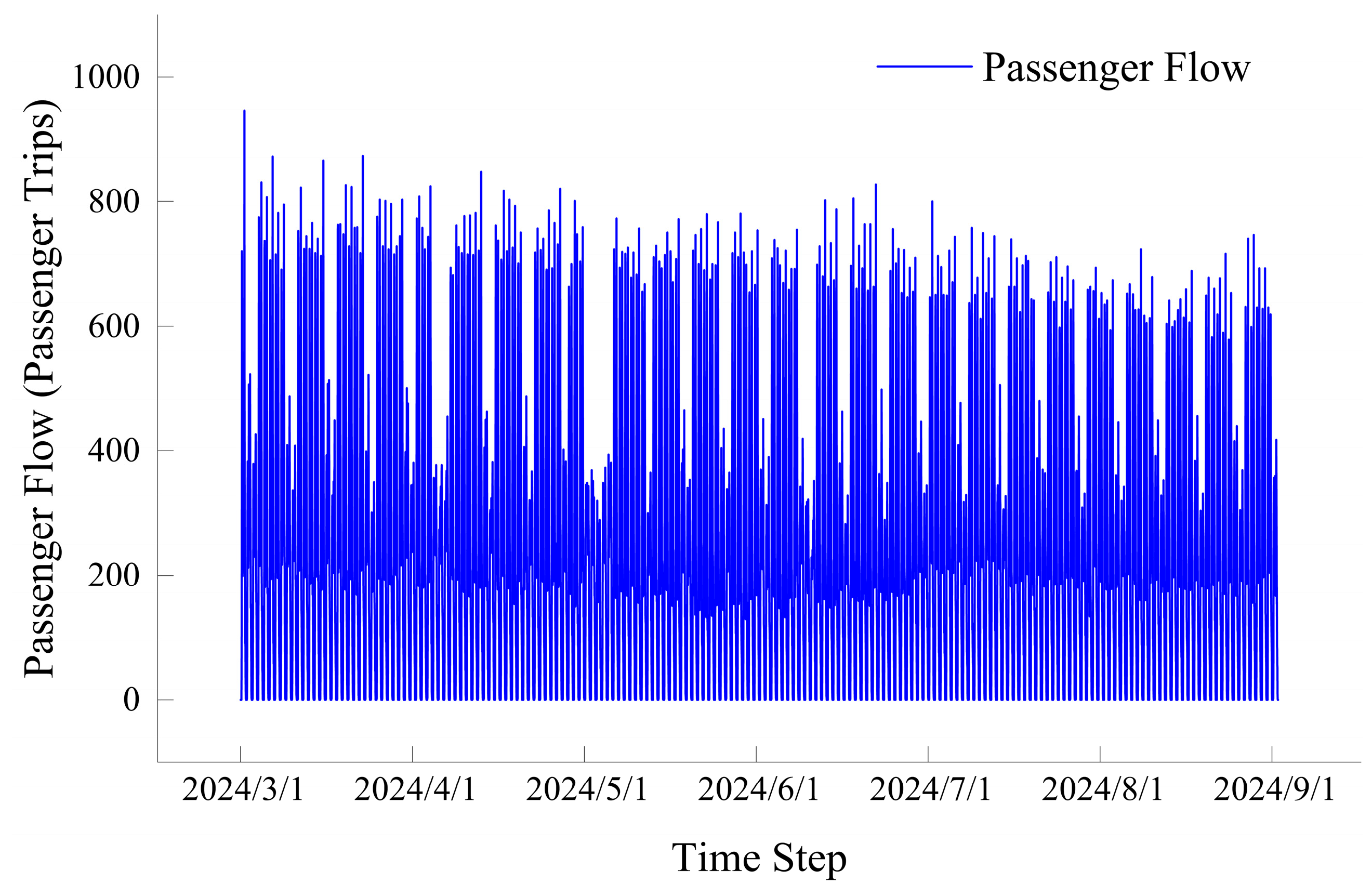
Building upon the previously constructed SMA-VMD-Informer-BiLSTM model, this paper conducts short-term entry passenger flow prediction based on the entry passenger flow data of Xi’an, Zhengzhou and Nanjing urban rail transit. We collected short-term entry passenger flow data from 300 subway stations in Xi’an Zhengzhou and Nanjing over a six-month period from 1 March 2024, to 31 August 2024. The data was aggregated in 30-min intervals, resulting in a total of 8832 data points for each station. The collected data was divided into time series, with the first 70% used as the training set and the remaining 30% as the test set for 48-step prediction. This paper initially focuses on Houweizhai Station, the starting station of Xi’an Metro Line 1, and performs short-term passenger flow prediction using its 30-min entry passenger flow data to validate the effectiveness of the model. Subsequently, predictions are made for multiple stations across different lines of the Xi’an, Zhengzhou and Nanjing subway system to further verify the model’s portability. Figure 3 presents the time-series plot of the passenger flow data at Houweizhai Station during this period. As can be observed from the figure, the passenger flow data during the study period exhibits significant nonlinear and non-stationary characteristics, providing an important reference basis for subsequent prediction analysis.

3.2. Model Preprocessing

To rigorously verify the effectiveness of the Simplified Moving Average (SMA) in optimizing the parameters of Variational Mode Decomposition (VMD), this study conducted a comparative analysis of the computational time consumption among four optimization algorithms—SMA, Particle Swarm Optimization (PSO), Genetic Algorithm (GA), and Bayesian Optimization—under identical computer hardware configurations. Specifically, focusing on the two key parameters in VMD, namely the number of modes K and the bandwidth constraint parameter α , optimization experiments were carried out using each of the four algorithms. To ensure the reliability and stability of the experimental results, each algorithm was independently trained 20 times, and the average training duration across these 20 trials was taken as the final training duration for comparative analysis. Detailed training duration data for each algorithm during the VMD parameter optimization process are presented in Table 2. Based on the analysis of the experimental results, this study confirms that, compared to the other three algorithms, the SMA employed in this paper exhibits a significant advantage in terms of training duration. Therefore, in the context of short-term passenger flow forecasting research presented in this paper, selecting SMA for parameter optimization of VMD demonstrates higher rationality and applicability.

3.3. Parameter Optimization

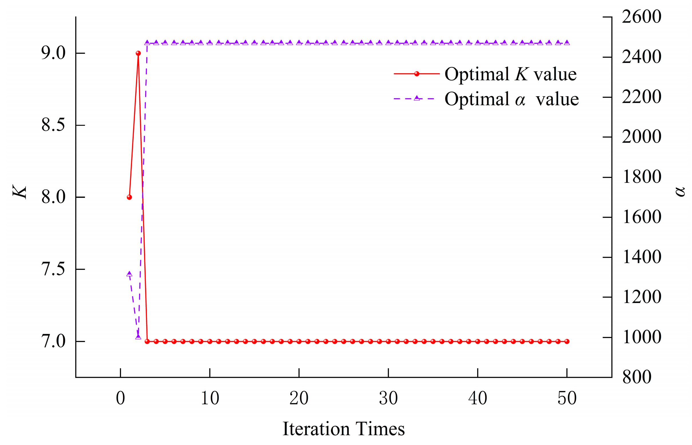
Prediction was conducted using the SMA-VMD-Informer-BiLSTM model, with the core hyperparameters employed in this study detailed in Table 3. These hyperparameters were selected based on an extensive review of relevant research literature in the field, representing critical factors in the model optimization process that significantly influence performance outcomes. To ensure optimal model performance under specific operational conditions and achieve accurate, efficient prediction and analysis, we conducted extensive experimental trials for hyperparameter tuning. Through multiple iterative experiments and precise adjustments, we successfully identified the optimal hyperparameter configuration tailored for the specific research target of Houweizhai Station, with detailed values presented in Table 3. The process of optimizing VMD parameters using SMA is illustrated in Figure 4.
The value range of K is set as integers within the interval [2, 10], while the range of α is defined as real numbers within [1000, 5000]. A total of 50 iterations is conducted. As can be observed from Figure 4, the optimal values of both the modal number K and the bandwidth constraint parameter α remain stable starting from the 3rd generation. Specifically, the optimal value of K eventually stabilizes at 7, and the optimal value of α finally stabilizes at 2469.324. Therefore, the optimal combination of K and α is set as (7, 2469.324).

3.4. Model Training

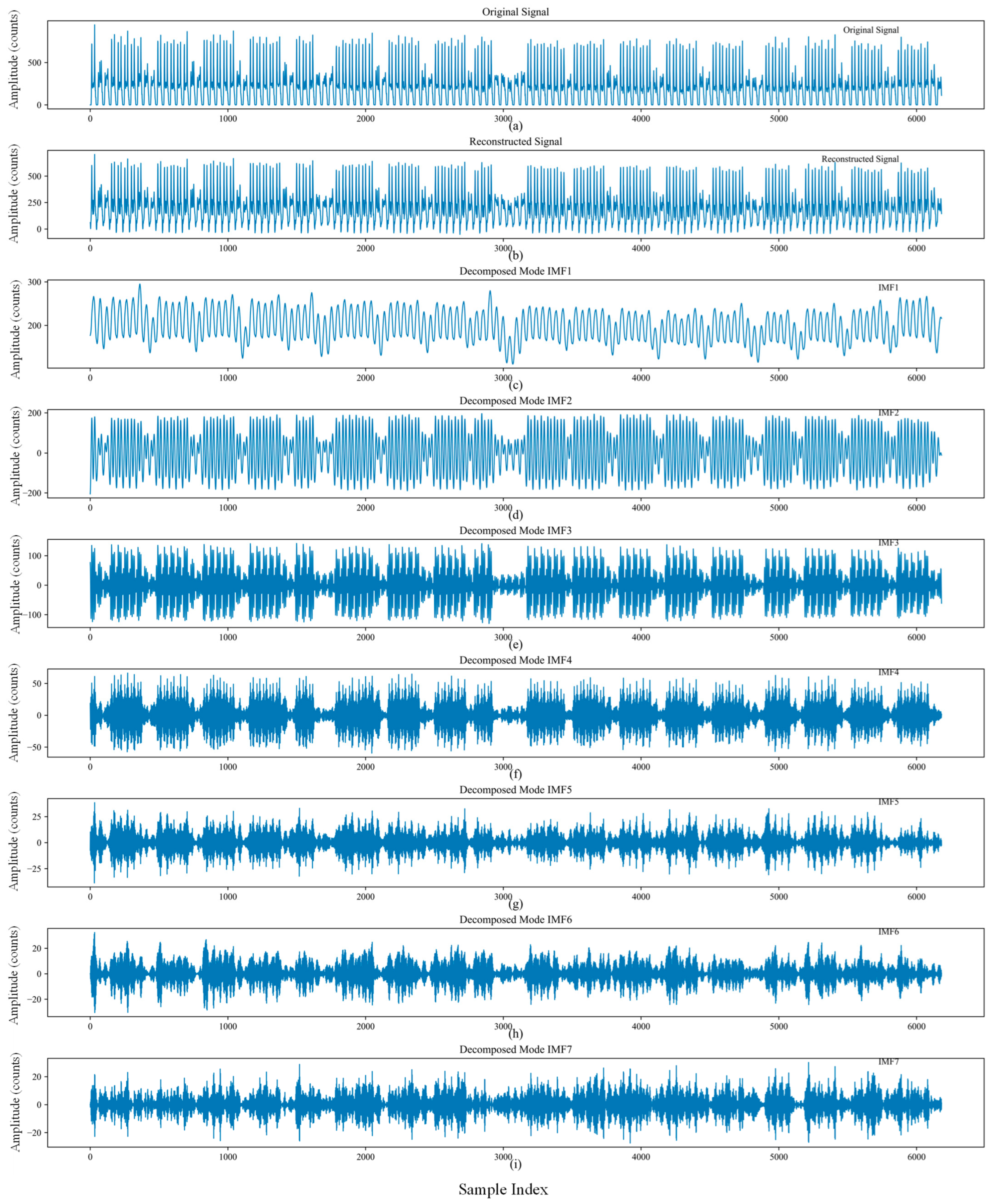
Figure 5 presents the decomposition results of the training set data by SMA-VMD. In the figure, the horizontal axis represents the sample points of the training set, with a total length of 6182, indicating the number of sample points. The vertical axis denotes the amplitude of the signal, and the ranges of the vertical axes in different subplots vary, reflecting the amplitude variations of different Intrinsic Mode Functions (IMFs). Specifically, Figure 5a shows the original passenger flow data signal, Figure 5b depicts the reconstructed signal, which is a combination of all IMFs, and Figure 5c–i display the seven decomposed modes, respectively, with each IMF representing a component of the signal within a specific frequency range. More precisely, IMF1 and IMF2 are high-frequency components of the signal, reflecting short-term fluctuations in the passenger flow data. IMF3, IMF4, and IMF5 represent relatively stable components, while IMF6 and IMF7 are low-frequency parts, reflecting the long-term trends of the passenger flow data. As can be seen from Figure 5, the reconstructed signal almost completely coincides with the original signal, demonstrating the excellent decomposition performance of VMD. Furthermore, each decomposed IMF contains distinct frequency components, indicating that VMD has successfully decomposed the original signal.
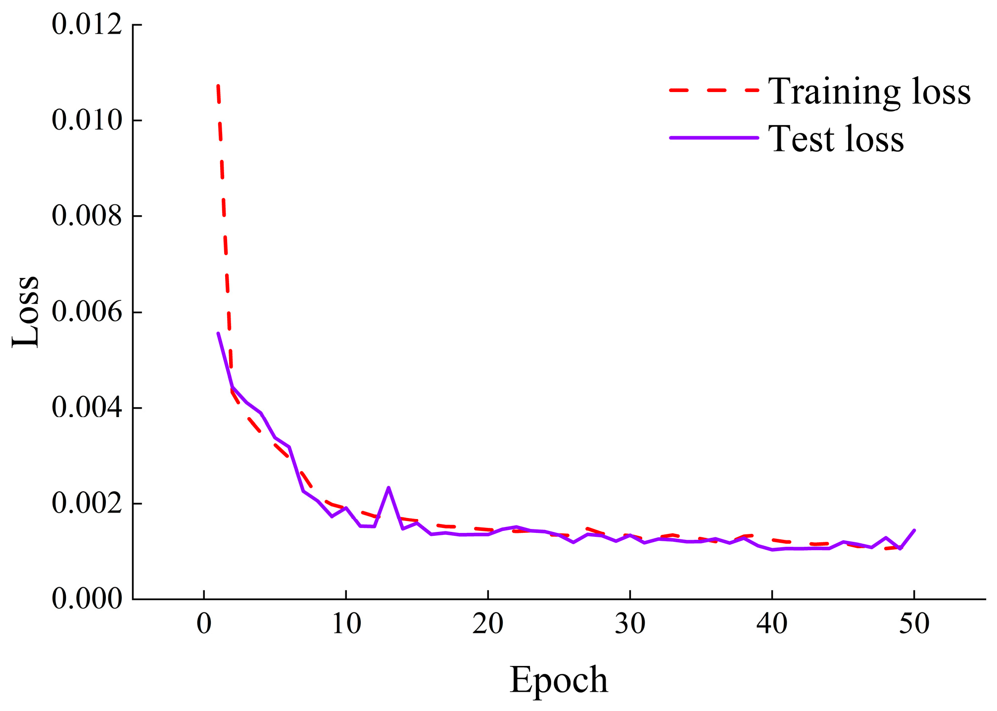
The loss variations of the SMA-VMD-Informer-BiLSTM model during the training process are illustrated in Figure 6. In the figure, the red dashed line represents the training set loss, while the purple solid line indicates the test set loss. It can be observed that the training set loss is relatively large in the initial stage but rapidly decreases and stabilizes, indicating a swift improvement and subsequent stabilization in the model’s fitting performance on the training set. Meanwhile, the test set loss is relatively small at the beginning, also drops quickly, and then levels off, reflecting the model’s strong generalization capability. Overall, the loss curves of the training set and the test set are very close to each other, suggesting that the model converges rapidly and performs well on both the training and test set data without experiencing overfitting or underfitting. This also demonstrates the excellent performance of the SMA-VMD-Informer-BiLSTM model in the task of short-term passenger inflow forecasting at stations.
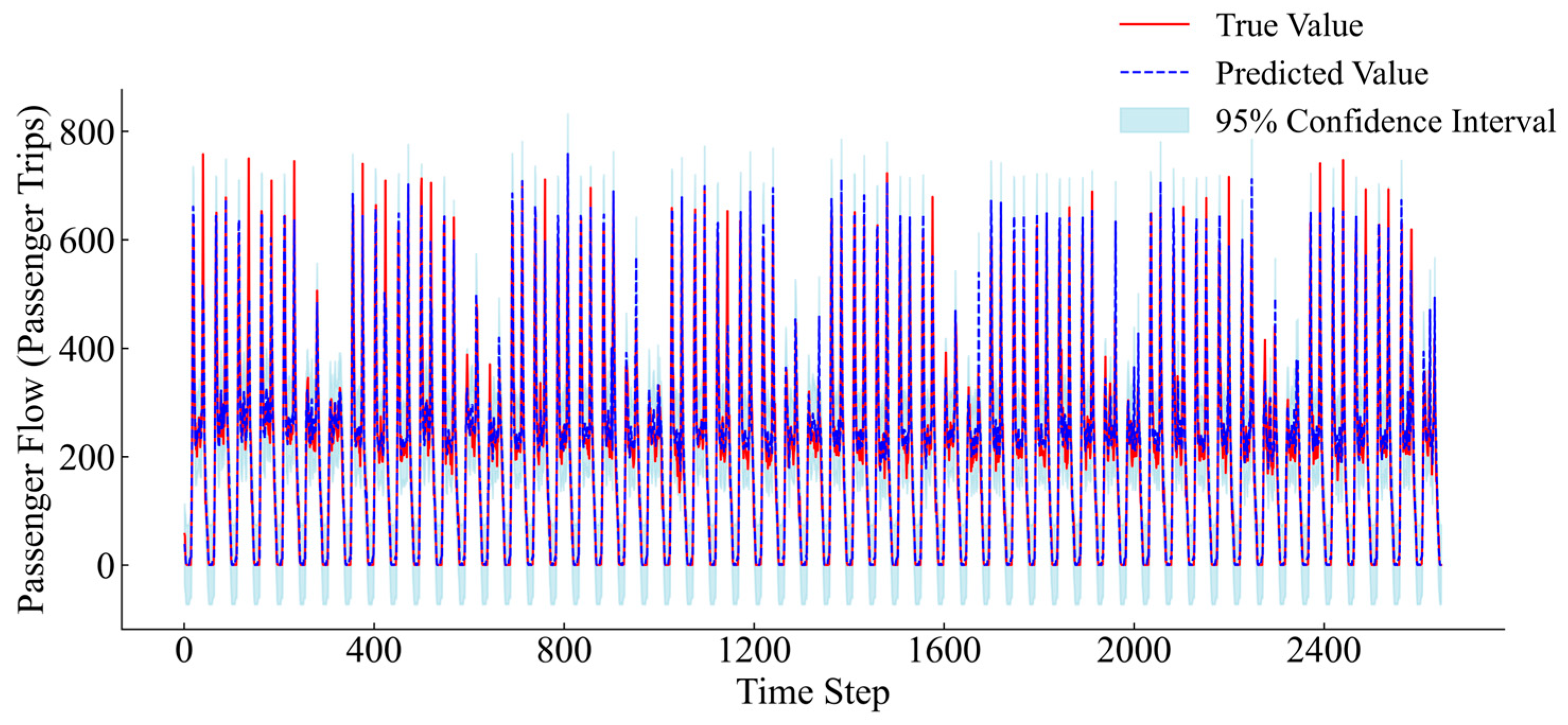
This paper conducts a visual analysis of the model’s prediction results on the test set. It plots the curves of the 48-step predicted values and the actual values, while also presenting the 95% confidence interval of the predicted values. The relevant results are shown in Figure 7. In the figure, the blue dashed line represents the trend of the predicted values for the test set, the red solid line reflects the changing trajectory of the actual values, and the 95% confidence interval of the predicted values is visually presented as a light blue area. By observing the figure, it can be found that the curve of predicted values largely overlaps with the curve of actual values, and the actual passenger flow curve consistently remains entirely within the 95% confidence interval. This indicates that the model’s prediction results are relatively accurate, and the predicted passenger flow data is basically consistent with the historical passenger flow data in terms of trends and patterns. This consistency demonstrates that the model can not only effectively capture the changing patterns of the current data but also has the capability to reasonably estimate future passenger flow trends.

3.5. Evaluation Metrics

To rigorously validate the effectiveness of the model, this paper has carried out a meticulous segmentation of passenger flow data at Xi’an Houweizhai Station. Specifically, based on the temporal characteristics of passenger flow, the data is divided into four representative time periods: morning peak period, evening peak period, weekend period, and holiday period. Subsequently, the model is employed to conduct passenger flow forecasting for each of the aforementioned time periods separately, and the model’s performance is quantitatively evaluated using error metrics such as f m s e , f r m s e and f m a e . The relevant error metric values are presented in Table 4. As can be seen from Table 4, the error metric values during the weekend period are significantly lower than those in other periods, reaching the minimum level. In contrast, the errors during the holiday period are relatively the largest. Meanwhile, the errors during both the morning and evening peak periods remain within a relatively small range. Analyzing the underlying causes, it is found that this phenomenon is closely related to the differences in passenger flow characteristics across different time periods. During weekends, people’s travel behaviors often exhibit strong regularity and stability, with relatively fixed elements such as travel purposes, travel times, and travel modes. This enables the model to more accurately capture the inherent patterns of passenger flow changes, thereby effectively reducing prediction errors. Conversely, during holidays, the composition of passenger flow becomes more complex. Factors such as the influx of non-local individuals, a surge in tourism-related travel demands, and the dispersion of travel times intertwine, leading to increased fluctuations in passenger flow data. Consequently, the error metric values during this period are higher than those in other periods. By comprehensively considering the error metric values across various time periods, including morning peak, evening peak, weekend, and holiday periods, it can be observed that the model demonstrates favorable predictive performance overall, with errors remaining at a relatively low level in each period. Combining this with the overall predictive effectiveness of the model on the test set as elaborated earlier, the following conclusion can be drawn: The model exhibits relatively excellent performance at Xi’an Houweizhai Station, possessing the capability to make accurate predictions in complex and variable passenger flow scenarios.

3.6. Results and Discussion

To verify the spatial portability of the SMA-VMD-Informer-BiLSTM model, this paper conducted 48-step forecasting of the 30 min interval passenger inflow data at multiple stations across various subway lines in Xi’an. By continuously adjusting the hyperparameters, the optimal results were obtained. Figure 8 illustrates the prediction results for the test sets of nine representative stations. Among them, Figure 8a–c encompass crucial subway transfer stations and scenic area stations, namely Fangzhicheng Station, Bell Tower Station, and Dayan Pagoda Station, in sequence. Figure 8d–f display railway and airport stations, specifically Xi’an North Railway Station, Xi’an Railway Station, and Airport Station, respectively. Figure 8g–i represent university stations and suburban stations, namely Northwestern Polytechnical University Station, Xi’an University of Science and Technology Station, and Qinling West Station. In the figures, the blue dashed line represents the predicted values for the test set, while the red solid line denotes the actual values. The 95% confidence interval of the predicted values is presented as a light blue area. It can be observed that there is a favorable fitting relationship between the predicted and actual values at each station, with the actual passenger flow curves consistently remaining within the 95% confidence interval. This indicates that the SMA-VMD-Informer-BiLSTM model constructed in this study demonstrates excellent performance in short-term passenger inflow forecasting for each station, thereby proving the model’s strong cross-station prediction capability.
The error metrics, including f m s e , f r m s e , f m a e , and the coefficient of determination R 2 , for each station are presented in Table 5. From an overall perspective of the error metrics, all values are relatively small, indicating robust predictive performance. Specifically, f m s e amplifies the impact of larger errors through squaring operations, making it particularly sensitive to sharp passenger flow fluctuations caused by large-scale events or temporary traffic controls. f r m s e , which shares the same unit as passenger volume, reflects the magnitude of global prediction deviations, while f m a e represents the average magnitude of prediction errors, indicating any systematic bias in the model’s predictions.
Notably, among these metrics, Northwest Polytechnical University Station exhibits the lowest values across all error indicators, followed by Xi’an University of Science and Technology Station. This can be attributed to the homogeneous passenger composition and regular travel patterns at stations near universities, which contribute to more predictable and stable passenger flow dynamics. Meanwhile, the passenger occupational distribution at Northwest Polytechnical University Station is more concentrated, whereas that at Xi’an University of Science and Technology Station is comparatively more dispersed. This disparity also contributes to the slightly higher prediction errors observed at Xi’an University of Science and Technology Station compared to Northwest Polytechnical University Station. Notably, the three stations with the highest f r m s e values are the airport, Xi’an Railway Station, and Xi’an North Railway Station. Similarly, the top three stations in terms of f m a e values are Xi’an Railway Station, the airport, and Xi’an North Railway Station. This phenomenon can be attributed to the fact that these three stations serve as major transportation hubs, characterized by a highly heterogeneous passenger composition and numerous surrounding interference factors. Consequently, the model’s fit to the specific characteristics of these stations is less precise than that for university stations.
The predictive performance exhibits variations across different stations. Nevertheless, on the whole, the model demonstrates commendable performance in forecasting passenger inflow data for Xi’an Metro. The prediction errors for stations such as Xi’an Railway Station and the airport remain within acceptable bounds. Moreover, the coefficient of determination R 2 values for all stations are notably close to 1, with Northwest Polytechnical University Station achieving the highest R 2 of 0.9971, and Xi’an Railway Station, despite having the lowest R 2 among all stations, still reaching a value of 0.9011. This evidence strongly supports a high degree of fit between the model’s predictions and the actual passenger inflow data at each station.
The aforementioned experimental results further substantiate that the proposed SMA-VMD-Informer-BiLSTM model is capable of effectively capturing the dynamic patterns of short-term passenger inflow in urban rail transit systems and providing accurate predictions of future passenger flow trends.
To comprehensively and thoroughly validate the predictive performance and generalization capability of the constructed model in cross-city and cross-station scenarios, this study selected representative urban stations for empirical analysis. Specifically, for Nanjing City, we chose Gulou Station (a downtown transfer station), Nanjing South Railway Station (a transportation hub), and Xianlin Road Station (a station in a university-concentrated area). Meanwhile, using the same data collection method, we selected Dongfeng Road Station, Zhengzhou East Railway Station, and Henan University of Technology Station in Zhengzhou City as research subjects for passenger inflow forecasting.
The prediction results of the test sets are presented in Figure 9a,b and Figure 10a,b. In these figures, the blue dashed line represents the trend of the predicted values for the test set, the red solid line indicates the trajectory of the actual values, and the 95% confidence interval of the predicted values is visually represented as a light blue area. Through the visual analysis, it can be observed that in the prediction results for each station, there is a high degree of fit between the predicted and actual values. The actual passenger flow curves consistently remain entirely within the 95% confidence interval. This indicates that the SMA-VMD-Informer-BiLSTM model constructed in this study can accurately capture the variation patterns of short-term passenger inflows and provide reliable prediction results when faced with various types of stations in different cities.
This empirical result strongly demonstrates that the model possesses robust cross-city and cross-station prediction capabilities. It can maintain high prediction accuracy and stability in complex and variable real-world scenarios, offering an efficient and reliable passenger flow forecasting method for the field of urban rail transit passenger flow prediction.

3.7. Comparison of Models

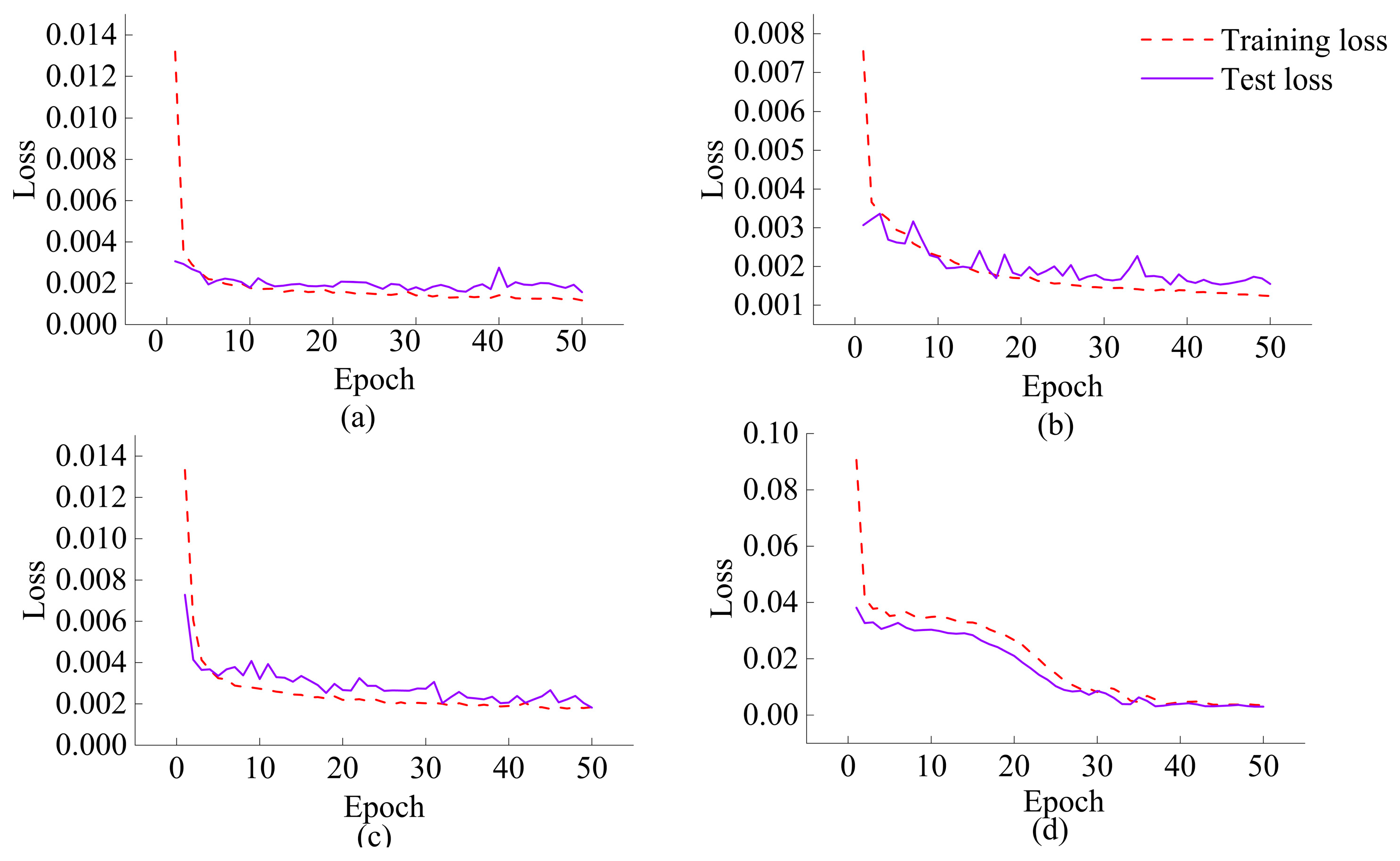
To further validate the effectiveness of the model, this paper compares the prediction results of the SMA-VMD-Informer-BiLSTM model with those of the CNN-BiLSTM, CNN-BiGRU, Transformer-LSTM, and ARIMA-LSTM models. The hyperparameters of these models were selected as the optimal parameter combinations under entirely consistent hardware environments, data partitioning methods, and evaluation metric systems. The loss function curves of each model are presented in Figure 11, where (a)–(d) successively depict the loss function graphs of the CNN-BiLSTM, CNN-BiGRU, Transformer-LSTM, and ARIMA-LSTM models. In the figures, the red dashed line represents the training set loss, while the purple solid line indicates the test set loss. In comparison with the training and test set loss function curves of the SMA-VMD-Informer-BiLSTM model shown in Figure 6, the loss function curves of the SMA-VMD-Informer-BiLSTM model essentially overlap after iterations, demonstrating a superior predictive performance.
Specifically, the evaluation metrics for each model are presented in Table 6. The SMA-VMD-Informer-BiLSTM model achieves an f m s e of 0.0014, an f r m s e of 0.0378, and an f m a e of 0.0226. Notably, compared to the CNN-BiLSTM, CNN-BiGRU, Transformer-LSTM, and ARIMA-LSTM models, the f m s e of the proposed model is reduced by 7.14–53.33%, the f m a e by 3.81–31.14%, and the f m a e by 8.87–38.08%. Furthermore, the R 2 of the proposed model reaches 0.9925, representing an improvement of 4.11–5.48% over the other models. These results indicate that the proposed model exhibits superior predictive performance in short-term passenger inflow forecasting tasks.

4. Conclusions

This study constructs a combined SMA-VMD-Informer-BiLSTM model to conduct 48-step forecasting of subway passenger inflows in Xi’an, Nanjing, and Zhengzhou. The experimental results demonstrate that the established model exhibits superior predictive accuracy and strong portability. Meanwhile, to enhance the credibility and practicality of the model in real-world decision-making, an in-depth exploration of the model’s interpretability, theoretical and practical value, as well as its limitations has been conducted. The specific conclusions are as follows:
(1)
Model methodology and performance advantages. This study presents a short-term passenger flow forecasting method. In this method, the parameters of VMD are optimized using the SMA, and the passenger inflow signals are decomposed accordingly. Subsequently, predictions are made through a combined Informer-BiLSTM model, and the results are output after fusion via a fully connected layer. Compared with traditional forecasting models, this proposed method demonstrates superior performance in terms of both various error metrics and the goodness-of-fit. From the perspective of interpretability, the process of SMA-optimized VMD parameter adjustment can automatically modify the number of decomposed modes and the central frequencies based on the inherent characteristics of passenger flow data. This enables the decomposed subsequences to better represent different patterns of passenger flow variations. The combined Informer-BiLSTM model, on the other hand, captures the temporal dependencies of passenger flow from both global and local perspectives. The fusion output through the fully connected layer allows the model to comprehensively consider the impacts of various factors on passenger flow, thereby providing operators with more credible forecasting results.
(2)
Model applicability and interpretability expansion. This model primarily centers on longitudinal temporal dependencies and is applicable to various types of rail transit stations. Particularly, when conducting real-time forecasting of passenger flows at stations with minimal external influence and strong regularity, such as those near universities, it exhibits remarkable applicability. From a theoretical standpoint, this is because the passenger flow variations at these stations display distinct periodicity and stability, which are highly congruent with the temporal dependencies captured by the model. In practical applications, the model can accurately predict passenger flows at different stations during various time periods, providing a scientific basis for operators to make rational arrangements for transportation capacity and personnel scheduling.
(3)
Subsequent research directions and model limitations. Under the premise of maintaining a single temporal dependency relationship unchanged, further capturing passenger flow abrupt changes through state-space reconstruction to enhance the dynamic response to transportation hub stations, and further exploring the group behavior patterns of different stations through state-transition modeling, represent directions for subsequent research. However, this study also has certain limitations. On the one hand, when dealing with passenger flow data under extreme circumstances, such as abnormal passenger flow fluctuations caused by sudden large-scale events or natural disasters, the prediction accuracy of the model may be compromised. This is because these extreme situations are characterized by uncertainty and complexity, which surpass the statistical patterns of the historical data on which the model is based. On the other hand, during the process of SMA-optimized VMD parameter adjustment, the model requires a substantial amount of computational resources and time. Future research will focus on addressing these issues, while also considering the use of multi-source data for prediction to further enhance the robustness and practicality of the model.

Author Contributions

Original data collection, writing, review, and editing were carried out by Y.L.; code development, writing, and manuscript preparation were performed by J.W. All authors have read and agreed to the published version of the manuscript.

Funding

This research was funded by the National Natural Science Foundation of China, grant number 72261025; the Natural Science Foundation of Gansu Province, China, grant number 23JRRA1690; the Soft Science Special Project of the Gansu Provincial Science and Technology Plan, grant number 25JRZA104; the Lanzhou Jiaotong University-Tianjin University Joint Innovation Fund Project, grant number 2022070; and the “Innovation Star” Project for Graduate Students in Higher Education Institutions of Gansu Province in 2025, grant number 2025CXZX-728.

Institutional Review Board Statement

Not applicable.

Informed Consent Statement

Not applicable.

Data Availability Statement

The data utilized in this research consists of inbound passenger flow data from Xi’an’s rail transit system in China. Due to specific reasons, the dataset is not available for public access.

Conflicts of Interest

The authors declare that they have no conflicts of interest.

References

  1. Macioszek, E. Analysis of the Rail Cargo Transport Volume in Poland in 2010–2021. Sci. J. Sil. Univ. Technol. Ser. Transp. 2023, 119, 125–140. [Google Scholar] [CrossRef]
  2. Khamis, A. Smart Mobility Education and Capacity Building for Sustainable Development: A Review and Case Study. Sustainability 2025, 17, 7999. [Google Scholar] [CrossRef]
  3. Xu, W.; Zhang, Y. Short-Term Passenger Flow Forecast of Rail Station Based on Random Forest Algorithm. J. Wuhan Univ. Technol. 2022, 46, 406–410. [Google Scholar]
  4. Lin, L.; Gao, Y.; Cao, B.; Wang, Z.; Jia, C. Passenger Flow Scale Prediction of Urban Rail Transit Stations Based on Multilayer Perceptron (MLP). Complexity 2023, 2023, 1430449. [Google Scholar] [CrossRef]
  5. Zhang, H.; Ma, W. Subway Passenger Flow Forecasting Model Based on Temporal and Spatial Characteristics. Comput. Sci. 2019, 46, 292–299. [Google Scholar]
  6. Deng, H.; Zhu, X.; Zhang, Q.; Zhao, J. Prediction of Short-Term Public Transportation Flow Based on Multiple-Kernel Least Square Support Vector Machine. J. Transp. Eng. Inf. 2012, 2, 84–88. [Google Scholar]
  7. Wang, X.; Zhang, N.; Zhang, Y.; Shi, Z. Forecasting of Short-Term Metro Ridership with Support Vector Machine Online Model. J. Adv. Transp. 2018, 2018, 3189238. [Google Scholar] [CrossRef]
  8. Yao, R.; Zhang, W.; Zhang, L. Hybrid Methods for Short-Term Traffic Flow Prediction Based on ARIMA-GARCH Model and Wavelet Neural Network. J. Transp. Eng. A Syst. 2020, 146, 4020086. [Google Scholar] [CrossRef]
  9. Li, L.; Wang, Y.; Zhong, G.; Zhang, J.; Ran, B. Short-to-Medium Term Passenger Flow Forecasting for Metro Stations Using a Hybrid Model. KSCE J. Civ. Eng. 2018, 22, 1937–1945. [Google Scholar] [CrossRef]
  10. Ma, C.; Li, P.; Zhu, C.; Lu, W.; Tian, T. Short-Term Passenger Flow Forecast of Urban Rail Transit Based on Different Time Granularities. J. Chang’an Univ. (Nat. Sci. Ed.) 2020, 40, 75–83. [Google Scholar]
  11. Ma, X.; Tao, Z.; Wang, Y.; Yu, H.; Wang, Y. Long Short-Term Memory Neural Network for Traffic Speed Prediction Using Remote Microwave Sensor Data. Transp. Res. Part C Emerg. Technol. 2015, 54, 187–197. [Google Scholar] [CrossRef]
  12. Zhang, H. Short-Term Passenger Flow Forecasting of Urban Rail Transit Based on Recurrent Neural Network. J. Jilin Univ. (Eng. Technol. Ed.) 2023, 53, 430–438. [Google Scholar]
  13. Liu, Y.; Liu, Z.; Jia, R. DeepPF: A Deep Learning Based Architecture for Metro Passenger Flow Prediction. Transp. Res. Part C Emerg. Technol. 2019, 101, 18–34. [Google Scholar] [CrossRef]
  14. Zeng, L.; Li, Z.; Yang, J.; Xu, X. Short-Term Passenger Flow Prediction Method of Urban Rail Transit Based on CEEMDAN-IPSO-LSTM. J. Railw. Sci. Eng. 2023, 20, 3273–3286. [Google Scholar]
  15. Zhang, B.; Yang, X.; Zhang, Y.; Li, D. Short-Term Inbound Passenger Flow Prediction of Model Rail Transit Based on Combined Deep Learning. J. Chongqing Jiaotong Univ. (Nat. Sci.) 2024, 43, 92–99. [Google Scholar]
  16. Gao, C.; Liu, H.; Huang, J.; Wang, Z.; Li, X.; Li, X. Regularized Spatial–Temporal Graph Convolutional Networks for Metro Passenger Flow Prediction. IEEE Trans. Intell. Transp. Syst. 2024, 25, 11241–11255. [Google Scholar] [CrossRef]
  17. Wang, J.; Ou, X.; Chen, J.; Tang, Z.; Liao, L. Passenger Flow Forecast of Urban Rail Transit Stations Based on Spatio-Temporal Hypergraph Convolution Model. J. Railw. Sci. Eng. 2023, 20, 4506–4516. [Google Scholar]
  18. Wang, X.; Xu, X.; Wu, Y.; Liu, J. Short Term Passenger Flow Forecasting of Urban Rail Transit Based on Hybrid Deep Learning Model. J. Railw. Sci. Eng. 2022, 19, 3557–3568. [Google Scholar]
  19. Alshehri, A.; Owais, M.; Gyani, J.; Aljarbou, M.H.; Alsulamy, S. Residual Neural Networks for Origin–Destination Trip Matrix Estimation from Traffic Sensor Information. Sustainability 2023, 15, 9881. [Google Scholar] [CrossRef]
  20. Owais, M. Deep Learning for Integrated Origin–Destination Estimation and Traffic Sensor Location Problems. IEEE Trans. Intell. Transp. Syst. 2024, 25, 6501–6513. [Google Scholar] [CrossRef]
  21. Li, S.; Chen, H.; Wang, M.; Heidari, A.A.; Mirjalili, S. Slime Mould Algorithm: A New Method for Stochastic Optimization. Future Gener. Comput. Syst. 2020, 111, 300–323. [Google Scholar] [CrossRef]
  22. Dragomiretskiy, K.; Zosso, D. Variational Mode Decomposition. IEEE Trans. Signal Process. 2014, 62, 531–544. [Google Scholar] [CrossRef]
  23. Wang, Y.; Lin, W.; Liang, Y.; Yang, J.; Li, A.; Diao, H. Railway Communication QoS Alarm Mechanism Based on XGBoost-Informer Model and Multi-Source Data. J. China Railw. Soc. 2024, 46, 86–96. [Google Scholar]
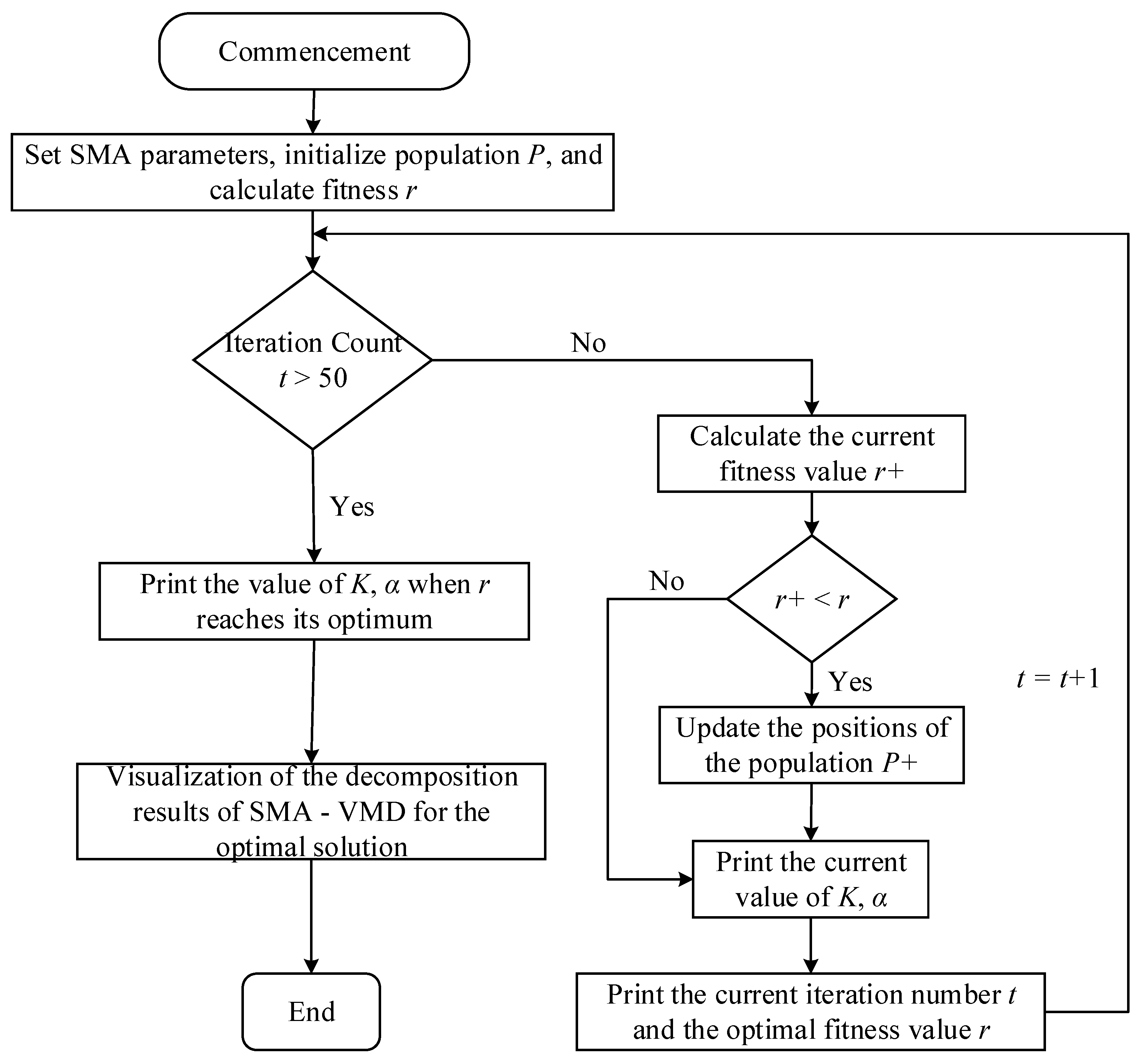
Figure 1. SMA-VMD flowchart.
Sustainability 17 08880 g001
Figure 2. Structure of SMA-VMD-Informer-BiLSTM.
Sustainability 17 08880 g002
Figure 3. Time-series chart of short-term inbound passenger flow at Houweizhai station.
Sustainability 17 08880 g003
Figure 4. The iterative process of optimizing VMD parameters using SMA.
Sustainability 17 08880 g004
Figure 5. SMA-VMD and reconstruction. (a) shows the original signal, (b) depicts the reconstructed signal, (ci) display the seven IMFs.
Sustainability 17 08880 g005
Figure 6. SMA-VMD-Informer-BiLSTM loss curve.
Sustainability 17 08880 g006
Figure 7. Test set prediction fitting.
Sustainability 17 08880 g007
Figure 8. Test set fitting of 48-step ahead prediction for various sites. (a) Fangzhicheng Station; (b) Bell Tower Station; (c) Giant Wild Goose Pagoda Station; (d) Xi’an North Station; (e) Xi’an Railway Station; (f) Xianyang International Airport Station; (g) Northwestern Polytechnical University Station; (h) Xi’an University of Science and Technology Station; (i) Qinling West Station.
Sustainability 17 08880 g008
Figure 9. Prediction for stations in Nanjing. (a) Gulou Station; (b) Nanjing South Railway Station; (c) Xianlin Road Station.
Sustainability 17 08880 g009
Figure 10. Prediction for stations in Zhengzhou. (a) Dongfeng Road Station; (b) Zhengzhou East Railway Station; (c) Henan University of Technology Station.
Sustainability 17 08880 g010
Figure 11. Comparison of model loss curves. (a) CNN-BiLSTM loss curve; (b) CNN-BiGRU loss curve; (c) Transformer-LSTM loss curve; (d) ARIMA-LSTM loss curve.
Sustainability 17 08880 g011
Table 1. Table of Comparison of Models in Related Studies on Short-Term Passenger Flow Forecasting in Urban Rail Transit.
ResearchModel MethodologyKey InnovationsPrediction Performance
Ma et al. [11]LSTMThis study represents the first application of LSTM networks to passenger flow forecasting.Achieved notable prediction accuracy, thereby pioneering the application of deep learning in passenger flow forecasting.
Zhang et al. [12]LSTM, GRUUtilized LSTM and GRU networks, respectively, to forecast passenger volumes at different station types during various time periods.Demonstrates robust predictive performance across diverse scenarios, illustrating the adaptability of different models to distinct data characteristics.
Liu et al. [13]LSTM—FC Integrated ModelIntegrates the sequential modeling capability of LSTM with the feature integration strength of fully connected layers.Effectively captures both long-term and short-term data dependencies, efficiently integrates and reduces high-dimensional feature dimensions, thereby enhancing prediction accuracy
Zeng et al. [14]CEEMDAN—IPSO—LSTM Integrated ModelThrough multi-scale feature extraction and hyperparameter optimizationSignificantly enhances the prediction accuracy and robustness of LSTM models
Li et al. [15]CNN—ResNet—BiLSTM ModelThrough multi-level feature fusion and deep residual networksFurther elevates prediction accuracy and noise resilience
Gao [16], Wang [17], Wang et al. [18]Integrated Model with Heterogeneous ArchitecturesPropose a Novel Architecture-Integrated ModelValidate the Effectiveness of a Heterogeneous Architecture-Integrated Model, Providing New Insights for Passenger Flow Prediction
Table 2. Comparative Table of Training Durations for Optimization Algorithms.
AlgorithmNumber of Training IterationsMean Training Time (min)
SMA2016.37
PSO2021.38
GA2053.91
Bayesian optimization2068.43
Table 3. Hyperparameters in the model.
HyperparameterValue
SMApopulation_size20
the upper bound is K , α [10, 5000]
The lower bound is K , α [2, 1000]
max_iter50
VMD f Original passenger flow data
α SMA optimum value
τ 0
K SMA optimum value
D C 0
i n i t 1
t o l 10−6
Informerenc_inIMFs
dec_inIMFs
seq_len96
label_len48
factor48
out_len48
BiLSTMhidden_layer_sizes[32, 64]
Training Hyperparametersbatch_size64
epochs50
learn_rate0.001
dropout0.3
Table 4. Error Metric Values for Different Time Periods.
Passenger Flow Periods f m s e f r m s e f m a e
Morning peak0.00450.06710.0412
Evening peak0.00250.05000.0289
Weekend0.00180.04240.0256
Holiday0.00750.08660.0572
Table 5. Evaluation metrics for each station.
Stations f m s e f r m s e f m a e R 2
Fangzhicheng0.00130.03640.02210.9876
Bell Tower0.00150.03850.02120.9708
Giant Wild Goose Pagoda0.00210.04610.02190.9686
Xi’an North Railway Station0.00620.07880.05270.9252
Xi’an Railway Station0.00980.09890.06970.9011
Xianyang International Airport0.01000.10000.06780.9114
Northwest Polytechnical University0.00090.03030.01960.9971
Xi’an University of Science and Technology0.00120.03530.02050.9954
Qinling West0.00300.05450.03280.9530
Table 6. Evaluation metrics of various models.
Models f m s e f r m s e f m a e R 2
SMA-VMD-Informer-BiLSTM0.00140.03780.02260.9925
CNN-BiLSTM0.00160.03960.02480.9489
CNN-BiGRU0.00150.03930.02510.9496
Transformer-LSTM0.00180.04260.02730.9409
ARIMA-LSTM0.00300.05490.03650.9517
Disclaimer/Publisher’s Note: The statements, opinions and data contained in all publications are solely those of the individual author(s) and contributor(s) and not of MDPI and/or the editor(s). MDPI and/or the editor(s) disclaim responsibility for any injury to people or property resulting from any ideas, methods, instructions or products referred to in the content.