Development of a Road Surface Conditions Prediction Model for Snow Removal Decision-Making

Abstract

Snowfall and road surface freezing cause traffic disruptions and skidding accidents. When widespread extreme cold events or sudden heavy snowfalls occur, the continuous monitoring and management of extensive road networks until the restoration of traffic operations is constrained by the limited personnel and resources available to road authorities. Consequently, road surface condition prediction models have become increasingly necessary to enable timely and sustainable decision-making. This study proposes a road surface condition prediction model based on CCTV images collected from roadside cameras. Three databases were constructed based on different definitions of moisture-related surface classes, and models with the same architecture were trained and evaluated. The results showed that the best performance was achieved when ice and snow were combined into a single class rather than treated separately. The proposed model was designed with a simplified structure to ensure applicability in practical operations requiring computational efficiency. Compared with transfer learning using deeper and more complex pre-trained models, the proposed model achieved comparable prediction accuracy while requiring less training time and computational resources. These findings demonstrate the reliability and practical utility of the developed model, indicating that its application can support sustainable snow removal decision-making across extensive road networks.

1. Introduction

1.1. Background

In cold-climate regions, precipitation occurs in various forms such as rainfall, snowfall, and frost. When rain or snow falls on the road surface, it may refreeze before evaporating, leading to surface freezing that appears as if a thin layer of ice were coating the pavement. Road surface freezing reduces the friction between tires and the pavement, leading to an increase in stopping distance [1]. Consequently, road surfaces covered with snow and ice pose a high risk of skidding accidents. In particular, black ice, which is hardly visible to drivers, is regarded as one of the most hazardous road surface conditions (RSC) by road maintenance authorities worldwide [2]. Previous research has shown that snowy weather patterns, such as snow accumulation, slush, or ice on pavements, account for about 24% of annual traffic crashes [3]. Other studies have reported that the frequency of multi-vehicle crashes increases during snowfall or blowing snow conditions [4]. In South Korea, large-scale accidents attributed to snowy weather and road surface freezing have occasionally occurred, including a 47-vehicle crash in 2019, a 41-vehicle crash in 2020, a 3-vehicle crash in 2022, and another 47-vehicle crash in 2023 [5,6].

On public roads, there are limited means of identifying RSCs beyond a driver’s visual observation, and localized phenomena such as road surface freezing are particularly difficult to detect from the driver’s field of view. Traditionally, RSC monitoring has relied on meteorological data from road weather information systems (RWIS) or manual patrolling by road authorities [7]. However, the high costs associated with installing and maintaining RWISs pose practical challenges [8]. In addition, it is practically impossible to monitor sporadically distributed vulnerable sections simultaneously through manual patrolling. Nevertheless, disasters caused by extreme cold weather, sudden heavy snowfall, and road surface freezing continue to occur, creating an urgent need for disaster risk reduction measures. Therefore, to prevent skidding accidents, road managers must be able to continue to make timely snow-removal decisions from the onset of snowfall and drops in temperature until the restoration of traffic systems. Accordingly, the development of a road surface condition prediction model applicable to extensive road networks is required.

1.2. Related Works

In the field of RSC prediction, various models have been developed using diverse methodological approaches. Representative RSC prediction approaches can be categorized into those based on numerical data collected under meteorological, traffic, and geographical conditions, and those based on road surface image data.

A study in Japan developed a Random Forest-based RSC prediction model using temperature, precipitation, traffic volume, and vehicle driving noise data, achieving over 94% classification accuracy [9]. In Canada, road surface temperature, air temperature, and precipitation data collected from RWISs were used as input for Model of the Environment and Temperature of Roads (METRo), and a methodology was proposed for predicting RSCs up to 24 h in advance [10]. In South Korea, Decision Tree, k-NN, and other machine learning algorithms were compared for RSC prediction, and in that study, the k-NN algorithm achieved 94% accuracy [11]. Each of these studies demonstrated notable results for RSC prediction models. However, since the models were developed using data collected under the specific conditions of each study area, their applicability may be limited when meteorological, traffic, or geographical conditions differ.

Meanwhile, image data-based models estimate RSCs from the visible form of surface moisture, allowing their application independently of meteorological and geographical conditions. Because training a convolutional neural network (CNN) from scratch demands extensive data and computational resources, an alternative approach is to utilize existing models whose performance has already been validated [12]. Consequently, numerous studies have investigated RSC prediction using transfer learning with pre-trained models. Transfer learning is a method in which the weights of an existing model are reused to accelerate the training process when learning data that are similar in nature to those used during the original training [13]. In transfer learning, the weights of a pre-trained model can be used as initial weights, and the method remains applicable even when the available training data are limited [14]. In the field of RSC prediction, ImageNet-based pre-trained models have been widely applied, with representative examples including AlexNet [15], VGG16 [16], Xception [17], Inception-V3 [18], ResNet50 [19], DenseNet169 [20], and MobileNetV2 [21]. However, because these models were originally developed for classifying a wide range of image categories, their application to RSC prediction—which typically involves a limited number of classes—may constitute an overly complex design. The increase in the number of operations in a model does not necessarily lead to a proportional increase in recognition accuracy [22]. Therefore, it is important to consider model architectures that can ensure sufficient performance with a practically acceptable computational cost.

RSCs can be broadly categorized into surfaces with moisture and those without. In winter, surfaces with moisture can be further classified based on the type and surface coverage of moisture, such as water, snow, and ice. In studies that considered the physical state of surface moisture, models trained using data under pure wet, ice, and snow conditions achieved strong performance [23]. Conversely, additional classes such as slushy or multiple hazards have been introduced to represent surfaces where multiple moisture states coexist beyond the three basic categories. However, studies have generally shown that the classification accuracy for these mixed conditions tends to be lower than that for other classes [24]. Another common approach to RSC classification is based on surface coverage, particularly the extent of snow accumulation. While distinguishing between snow-free and snow-covered surfaces tends to yield high classification accuracy, model performance tends to degrade as the snow-covered classes are subdivided more finely [25].

Since the models developed in each study differ in terms of network architecture, data quality, and preprocessing methods, it is difficult to make direct comparisons of model performance. However, it has been observed that the classification accuracy of models can vary depending on how the classes are defined, and that overly fine-grained class distinctions may lead to an increase in prediction errors.

2. Research Methodology

As discussed in the literature, various approaches can be considered for RSC prediction. However, numerical data-based models require the collection of extensive meteorological data, such as air temperature and road surface temperature. In particular, road surface temperature exhibits large variations across different sections, which may require an excessive number of sensors for data collection. Moreover, numerical data-based models have limitations in terms of scalability to other conditions. Therefore, in this study, RSC prediction models were developed using a CNN-based approach with image data.

CNN algorithms have been successfully applied across a wide range of domains, supported by the availability of large-scale image datasets such as ImageNet and the advancement of high-performance GPUs [26,27]. In line with this trend, various approaches have been explored, including the development of new CNN models, and the application of transfer learning using pre-trained CNN architectures [7,24,28]. However, most existing studies have focused on applying complex and highly advanced models, and relatively little attention has been given to approaches from the perspective of road managers who are expected to utilize such models in practice. Therefore, it is necessary to simplify the model so that it can be readily applied in practice. In addition, for application to RSC prediction, it is necessary to analyze whether a lightweight model can offer comparative advantages in terms of performance and speed compared with complex transfer learning-based models.

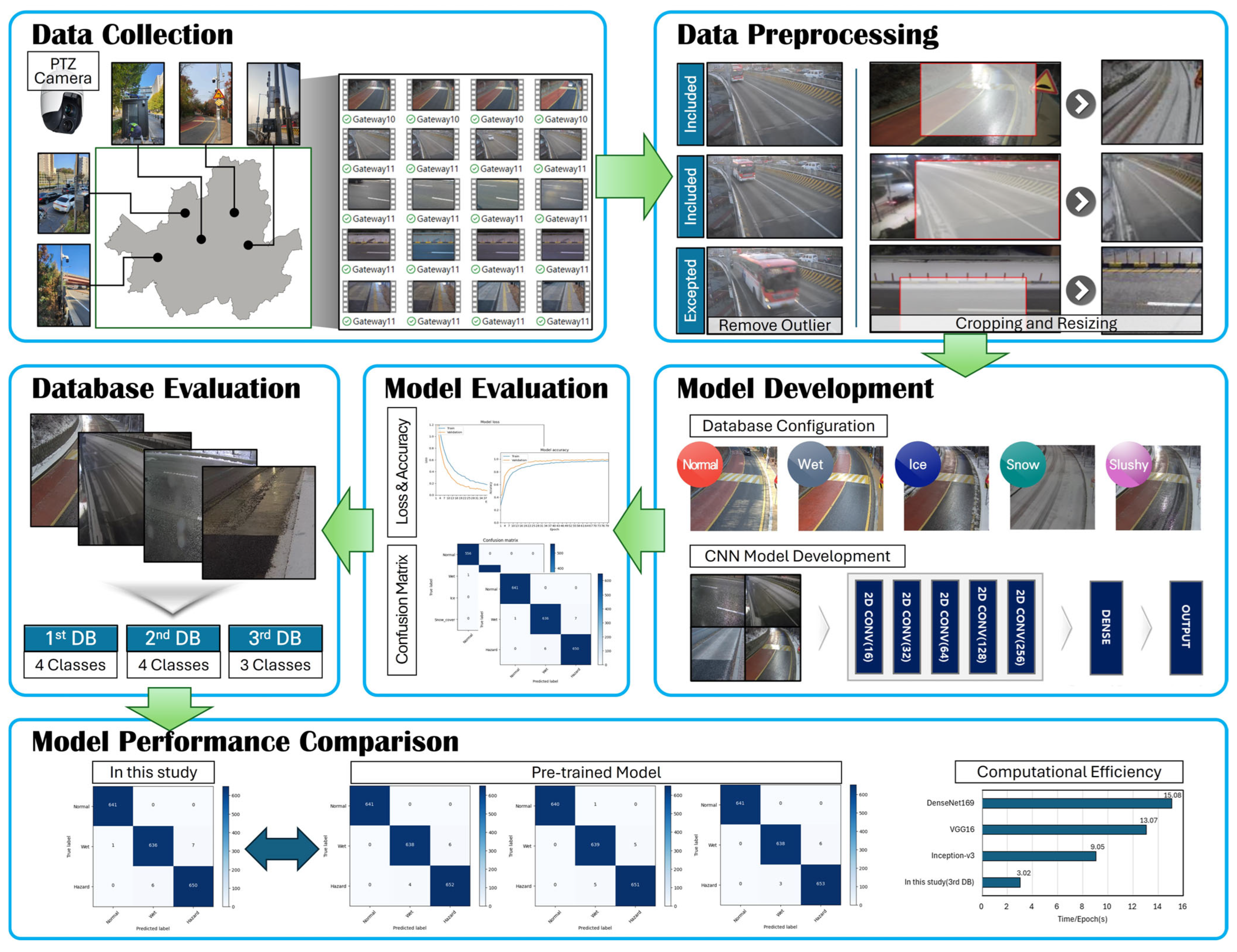
In this study, the methodology was established as illustrated in Figure 1. First, video data of winter road surfaces were collected from five locations in Seoul, South Korea. The collected video data were preprocessed and extracted as still images. Based on a CNN algorithm with a simplified architecture, an RSC prediction model was developed and trained using the extracted images. The training results were then compared according to the type of database, with the aim of identifying the most suitable database structure and model configuration from the perspective of practical use by road managers. Finally, the performance of the lightweight model was evaluated through comparison with pre-trained models developed through transfer learning, based on the data used in this study.

3. RSC Prediction Model Development

3.1. Data Collection and Preprocessing

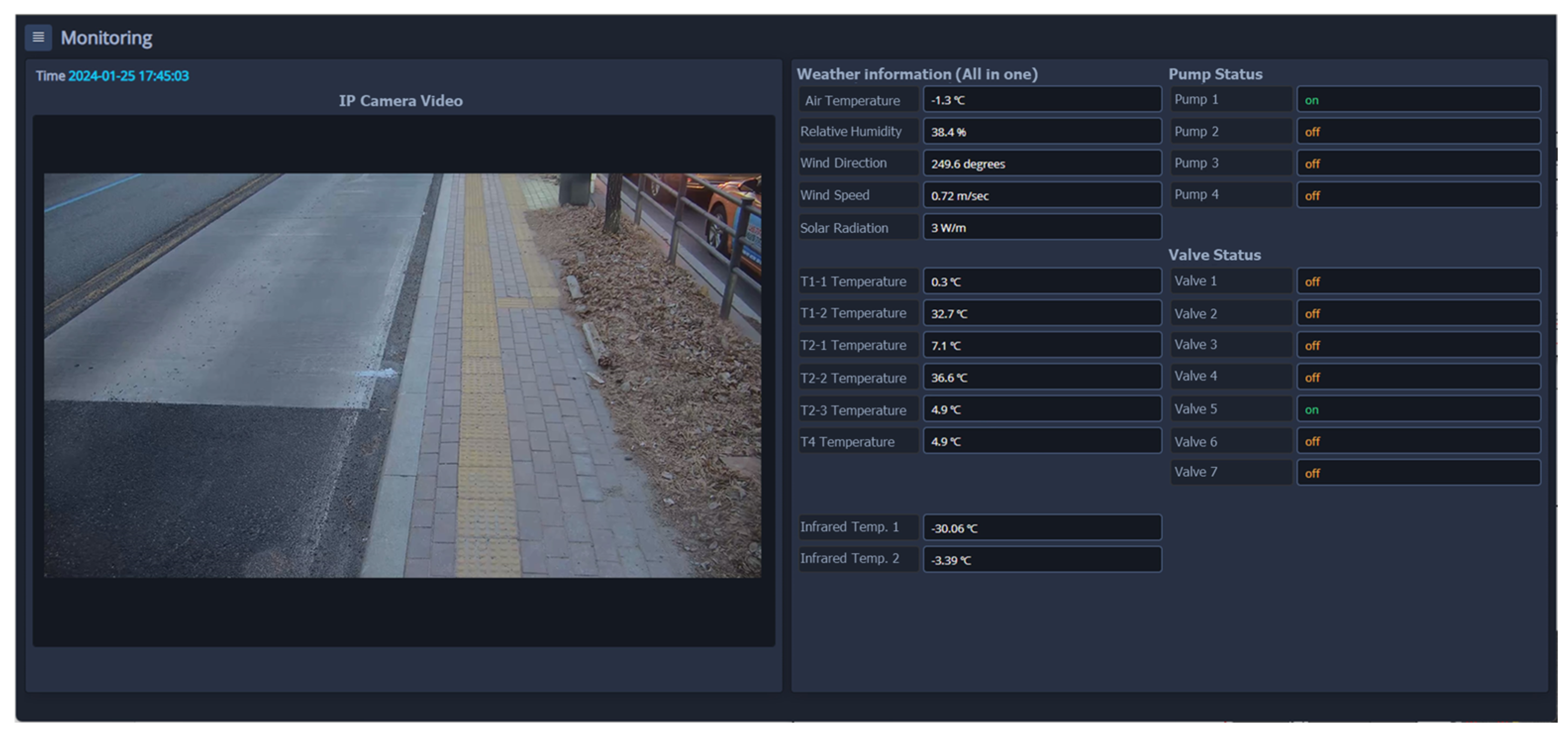
In this study, CCTV cameras of the type commonly used in road environments in South Korea were utilized to collect road surface videos over a period of approximately three months. Figure 2 shows a panoramic view of the five sites where the cameras were installed. To prevent variations in prediction performance due to differences in pavement materials, CCTV cameras were installed at three asphalt-paved sites and two concrete-paved sites to ensure a balanced dataset.

The data transmission interval and video length were determined in consideration of practical factors such as communication costs and server performance. The weather conditions in the data collection areas were generally clear, with occasional rainfall or snowfall. Therefore, to prevent data imbalance, it is necessary to collect data at shorter time intervals when rainfall or snowfall occurs. In this study, the camera recording interval was set to range from a minimum of 10 min to a maximum of 2 h, allowing more frequent data collection during precipitation events. In addition, each recording captured a 10-s video, which was transmitted to the server in real time, as shown in Figure 3. The cameras used in this study are capable of recording at 30 frames per second, making it possible to extract up to 300 still images from each video transmitted to the server.

The road surface videos transmitted to the server were preprocessed for use as training data. First, in order to enhance model performance and minimize bias, any video that included obstacles such as people or vehicles that blocked the view of the road were defined as an outlier and excluded from the training dataset. However, since the video data were collected from public roads, obtaining completely unobstructed data was practically difficult. Therefore, video segments were included in the training dataset as long as the road surface remained identifiable, even if vehicles were present in the frame. Based on this criterion, Figure 4 presents examples of video frames that were included in the training dataset and those that were excluded. The 10-s video clips captured a variety of scenes depending on the presence or movement of vehicles. Figure 4a,b show cases where no vehicles are present or only a small portion is captured, allowing the RSCs to be clearly observed. These were included in the training dataset. In contrast, when a vehicle approached the CCTV and obscured most of the road surface—as shown in Figure 4c—the image was considered an outlier that could not be used for training. Such data were excluded from the training dataset, as they were judged as likely to degrade the performance of the prediction model.

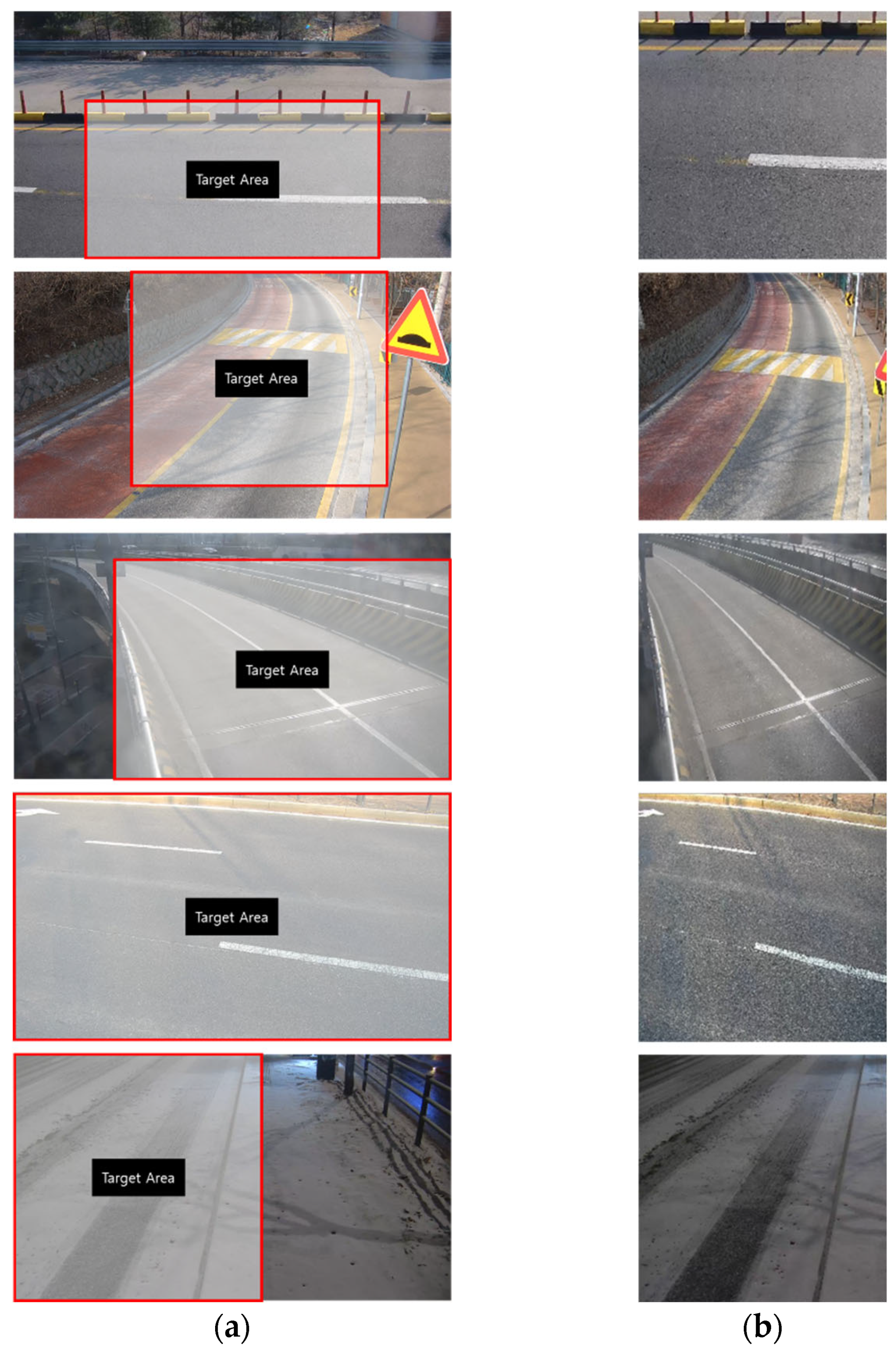
Next, to enhance the image feature learning and classification performance of the CNN model, a target area corresponding to the road surface was defined and extracted. The target area was determined based on the camera angles at each site. As shown in Figure 5a, the original data and the designated target area are indicated. Roadside facilities such as sidewalks, and signposts were excluded as much as possible, and the area was selected to focus on the main roadway. Meanwhile, convolutional neural networks require all input images to be of uniform size. However, since general images typically vary in dimensions, preprocessing steps such as cropping the target area and resizing are necessary [29]. In this study, the extracted target areas were resized to a square resolution of 256 × 256 pixels. The result of this preprocessing is shown in Figure 5b.

3.2. Data Configuration

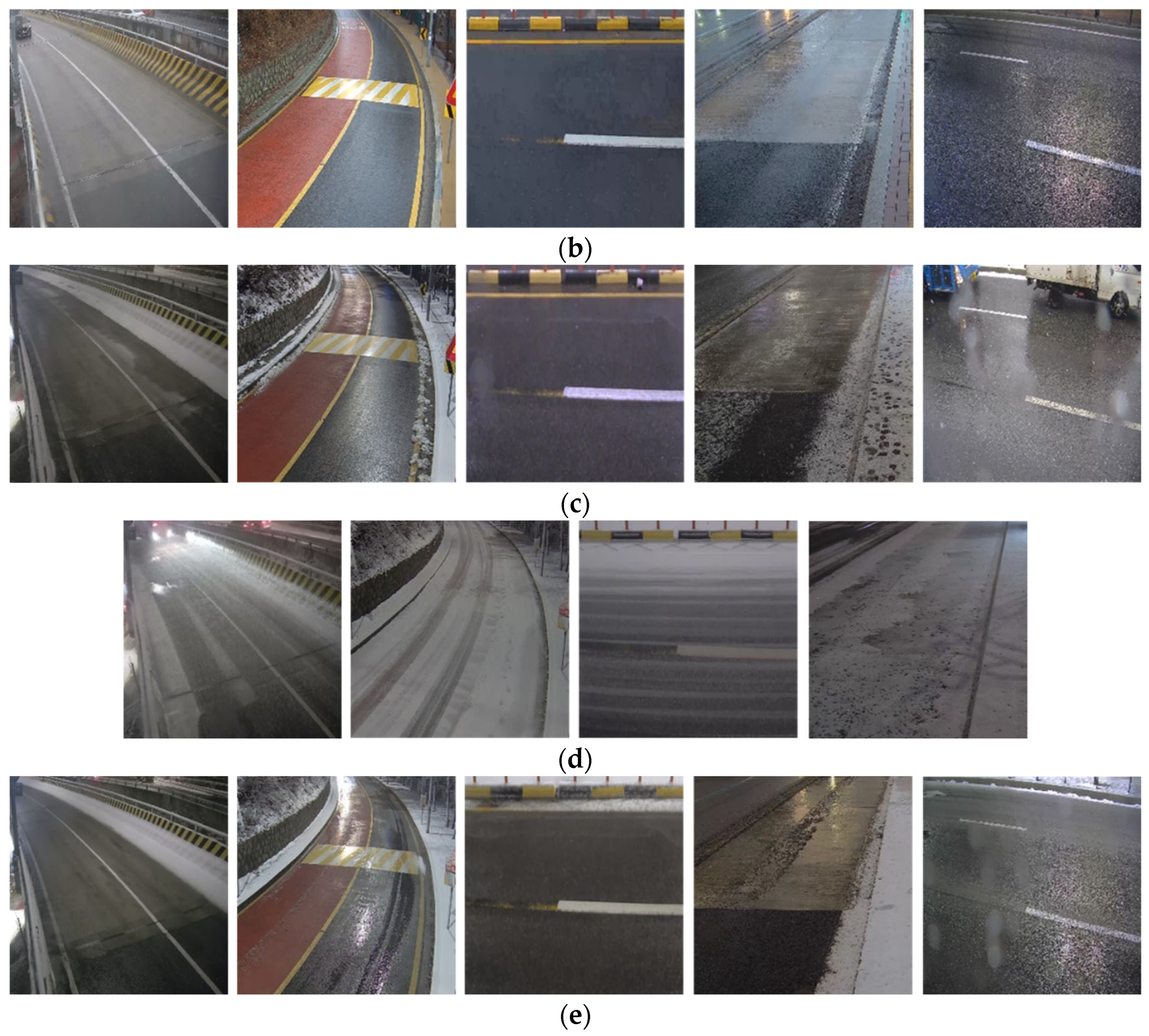
For preventing skidding accidents, RSCs can be visually classified into the following categories: conditions with little to no moisture, conditions where moisture is present in the form of water, conditions where moisture is present as ice, and conditions where moisture appears as snow. Figure 6a–d show examples from the collected dataset in which the RSCs can be intuitively distinguished based on the form of surface moisture. In Figure 6d, one site (shown in Figure 2a) did not present a snowy road during the data collection period of this study. Additionally, because temperatures during winter often fluctuate above and below freezing, snow that has accumulated on the road surface may repeatedly melt and refreeze. As a result, road surfaces are more frequently found in a slushy conditions—where water, ice, and snow coexist, as shown in Figure 6e—rather than in a clearly defined icy condition when freezing occurs.

The criteria for defining the slushy condition as a distinct class can vary depending on the objectives and methods of each study [24,25]. In practice, road surface monitoring through CCTV images relies on visual inspection by personnel. Accordingly, in this study, the collected video data were labeled based on the visually identified proportions of surface moisture conditions. The labeling criteria for each database type are summarized in

Table 1. Classification of Road Surface Condition (RSC) for Database Construction.

No. of DB	RSC	Definition
1st DB	Normal	Completely dry or nearly dry condition
	Wet	A condition in which the area covered by water among the moisture present on the road surface is the largest
	Ice	A condition in which the area covered by ice among the moisture present on the road surface is the largest
	Snow	A condition in which the area covered by snow among the moisture present on the road surface is the largest
2nd DB	Normal	Completely dry or nearly dry condition
	Wet	A condition in which the moisture present on the road surface exists only in the form of water
	Ice	A condition in which the area covered by ice among the moisture present on the road surface is larger than that covered by snow
	Snow	A condition in which the area covered by snow among the moisture present on the road surface is larger than that covered by ice
3rd DB	Normal	Completely dry or nearly dry condition
	Wet	A condition in which the moisture present on the road surface exists solely in the form of water
	Hazard	A condition in which ice or snow is present on the road surface

, and three databases were developed from the same training data using three distinct class determination methods.

In the first database, slushy surfaces were classified as wet, ice, or snow based on the visually observed relative surface coverage of water, ice, and snow. In the second database, as in the first, slushy surfaces were classified as either ice or snow by comparing their respective coverage while disregarding water. This approach prioritizes ice or snow classification even when their surface coverage is smaller than that of wet, because icy and snowy roads pose a higher risk of traffic accidents. In the third database, ice, snow, and slushy conditions were grouped into a single class called hazard, focusing on the risk of skidding accidents rather than the specific state of surface moisture. Road surfaces in ice, snow, or slushy conditions all pose a high risk of skidding accidents. Therefore, from the perspective of road management, snow removal operations tend to be initiated for any hazardous condition, regardless of the specific form of surface moisture. Since the objective of this study is to develop an automated classification model that supports road managers in promptly identifying road surfaces with a high risk of slipping, the third database is considered the most aligned with the study’s goal. Depending on the research objectives and the data collection environment, slushy conditions can be defined as a single class. However, in this study, because the data moisture conditions were insufficient compared to normal, slushy conditions were not treated as an independent class to prevent potential model performance degradation caused by data imbalance.

The composition of the training data based on the classification criteria in Table 1 is summarized in

Table 2. Summary of Datasets for Model Development.

Category		Train		Valid			Test
		Dataset	Ratio (%)	Dataset		Ratio (%)	Dataset	Ratio (%)
1st DB	Normal	1836	26	484		27	580	27
	Wet	1830	26	445		26	568	26
	Ice	1712	25	410		24	530	24
	Snow	1608	23	408		23	503	23
	Sum	6986	100	1747		100	2181	100
	Subtotal (Train + Valid)				8733 (Asphalt: 4918; Concrete: 3815)
	Total (Train + Valid + Test)				10,914 (Asphalt: 6176; Concrete: 4738)
2nd DB	Normal	1769	25	457		26	556	26
	Wet	1806	26	446		26	562	26
	Ice	1743	25	417		24	539	25
	Snow	1658	24	425		24	520	23
	Sum	6976	100	1745		100	2177	100
	Subtotal (Train + Valid)				8721 (Asphalt: 4848; Concrete: 3873)
	Total (Train + Valid + Test)				10,898 (Asphalt: 6090; Concrete: 4808)
3rd DB	Normal	2121	33	529		33	641	33
	Wet	2135	33	527		33	644	33
	Hazard	2149	34	546		34	656	34
	Sum	6405	100	1602		100	1941	100
	Subtotal (Tarin + Valid)				8007 (Asphalt: 4484; Concrete: 3523)
	Total (Train + Valid + Test)				9948 (Asphalt: 5599; Concrete: 4349)

. Although the total number of images varies slightly across databases depending on the number of classes and their definitions, each database was prepared to contain approximately 10,000 images. In addition, the quantity of data for each class was balanced within each database to prevent class imbalance. Additionally, the ratio of asphalt to concrete pavement data was approximately 55%:45%. To avoid overfitting and ensure effective learning, each database was divided into train, validation, and test sets at a ratio of approximately 65%:15%:20%.

3.3. RSC Prediction Model Architecture and Training Environment

In this study, the number of RSC classes was limited to no more than five. From the perspective of road managers, it is necessary to reduce the time required for real-time RSC prediction in order to enable prompt decision-making. Therefore, the model structure was simplified to reduce the prediction time of RSCs across an extensive road network.

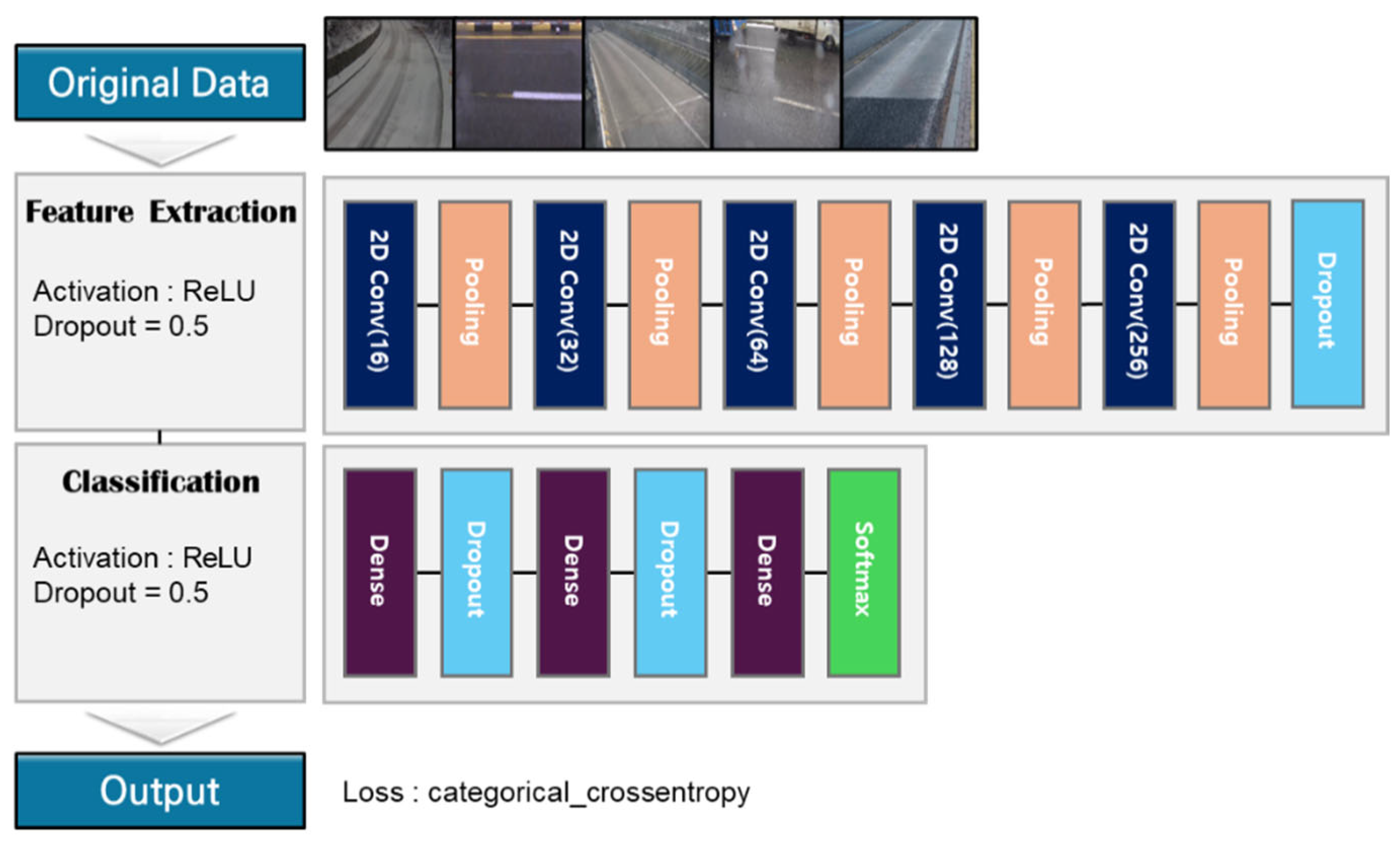
In this study, the model was implemented using TensorFlow and Keras (version 2.10.0), widely used Python-based deep learning frameworks. The system was equipped with an NVIDIA GeForce RTX 4070ti GPU. Figure 7 and

Table 3. Model Summary.

Layer	Output Shape	Number of Parameters
Conv2D (3 × 3)	(254, 254, 16)	((3 × 3 × 3) + 1) × 16 = 448
Max-pooling (2 × 2)	(127, 127, 16)
Conv2D (3 × 3)	(125, 125, 32)	((3 × 3 × 16) + 1) × 32 = 4640
Max-pooling (2 × 2)	(62, 62, 32)
Conv2D (3 × 3)	(60, 60, 64)	((3 × 3 × 32) + 1) × 64 = 18,496
Max-pooling (2 × 2)	(30, 30, 64)
Conv2D (3 × 3)	(28, 28, 128)	((3 × 3 × 64) + 1) × 128 = 73,856
Max-pooling (2 × 2)	(14, 14, 128)
Conv2D (3 × 3)	(12, 12, 256)	((3 × 3 × 128) + 1) × 256 = 295,168
Max-pooling (2 × 2)	(6, 6, 256)
Dropout (0.5)	(6, 6, 256)
Flatten	(9216)
Dense (FC)	(48)	(9216 × 48) + 48 = 442,416
Dropout (0.5)	(48)
Dense (FC)	(24)	(48 × 24) + 24 = 1176
Dropout (0.5)	(24)
Dense (FC)	(4)	(24 × 4) + 4 = 100
Total Parameters		836,300

summarize the architecture and layer-wise configuration of the CNN model developed in this study. The model consists of two main components: a feature extraction stage and a classification stage.

The feature extraction stage consists of five convolutional layers. When a (256 × 256) pixels is provided as input, the model iteratively applies convolution and pooling operations to extract features from the image. Various pooling approaches exist, such as average pooling, min-pooling, and fractional max-pooling. In this study, max-pooling, which is widely recognized as one of the most effective techniques in image and video recognition, was adopted [30]. Additionally, the activation function used in the feature extraction layers was the Rectified Linear Unit (ReLU). As the input data pass through the convolution and pooling operations, the CNN model extracts progressively deeper and higher-dimensional features. At the same time, the size of the output data becomes gradually smaller.

The classification stage comprises three fully connected layers, with the ReLU activation function consistently applied, as in the preceding stage. However, the final layer uses the softmax activation function, which is commonly employed in classification involving three or more classes. In this stage, the three-dimensional tensor output from the feature extraction stage is flattened into a one-dimensional vector, and then passed through the three fully connected layers to predict the class of the input data. Early stopping and dropout were applied during the classification stage to prevent overfitting. The specific hyperparameter values used in the model are summarized in

Table 4. Hyperparameter Configuration.

Hyperparameter	Value
Kernel Size	3 × 3
Max-pooling	2 × 2
Learning rate	0.001
Dropout rate	0.5
Optimizer	SGD (lr = 0.001, momentum = 0.9, Nesterov = Ture)
Epoch	80
Batch size	32
Early-stopping	5

.

4. Comparison of RSC Prediction Models According to Database Type

4.1. Training and Validation

Using the CNN model developed in this study, road surface images from the three databases were used for model learning. To evaluate the training results, the train and validation sets of the dataset were used to derive the model loss and accuracy, and the confusion matrix.

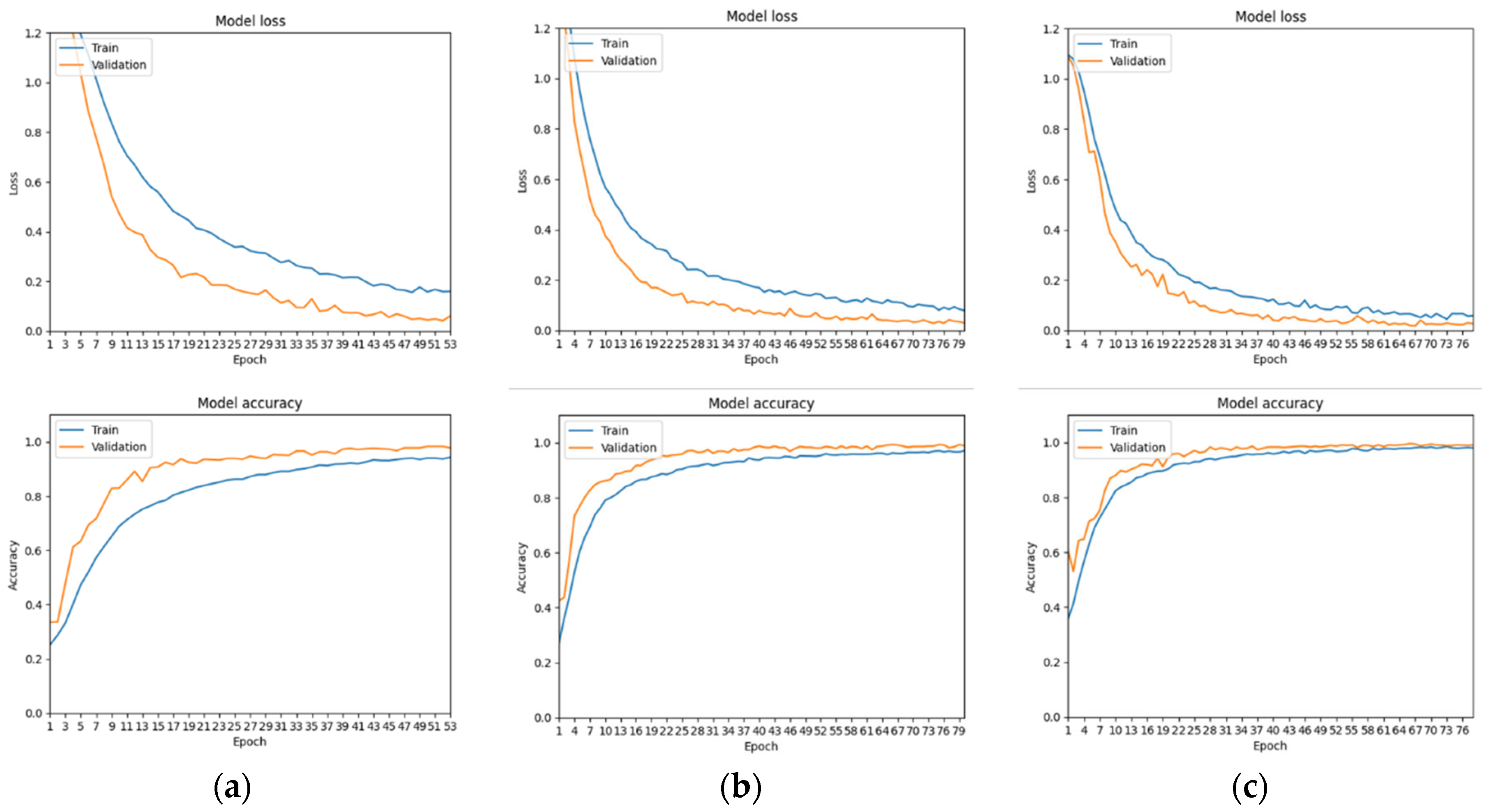
First, Figure 8 and

Table 5. Training Results of CNN Models.

Category	1st DB	2nd DB	3rd DB
Train Loss	0.1594	0.0793	0.0581
Validation Loss	0.0613	0.0295	0.0263
Train Accuracy	94.29%	97.05%	98.00%
Validation Accuracy	97.71%	98.85%	99.06%

summarize the training results for the databases used in model development. For the first database, early stooping was applied to prevent overfitting. Across all databases, the validation loss was lower and the validation accuracy was higher than in the train set. This result can be attributed to the high dropout rate. Additionally, the validation accuracy for all databases exceeded 97%, indicating strong classification performance. However, the first database, in which slushy surfaces were classified as wet, ice, or snow based on their relative surface area, showed the highest loss and the lowest accuracy. In contrast, the third database, where ice, snow, and slushy were grouped into a single hazard class, demonstrated the best performance.

4.2. Evaluation of Prediction Performance

Figure 9 and

Table 6. Comparison of Performance of Models.

Category	RSC	Precision	Recall	F1-Score	Support
1st DB	Normal	1.00	1.00	1.00	580
	Wet	0.97	1.00	0.98	568
	Ice	0.99	0.96	0.98	530
	Snow	1.00	0.99	0.99	503
2nd DB	Normal	1.00	1.00	1.00	556
	Wet	0.98	0.99	0.99	562
	Ice	0.99	0.96	0.98	539
	Snow	0.98	0.99	0.99	520
3rd DB	Normal	1.00	1.00	1.00	641
	Wet	0.99	0.99	0.99	644
	Hazard	0.99	0.99	0.99	656

present the model’s prediction performance, evaluated using the confusion matrix for the test set of each database. In Figure 9, the vertical axis represents the actual data classes, while the horizontal axis shows the classes predicted by the model. In all cases, the model achieved consistently high accuracy in classifying the test data classes. In particular, predictions for the normal class were completely accurate in all cases except for a single misclassification in the first database.

In the first and second databases, most prediction errors occurred in the classification of the ice class. Specifically, in the first database, most errors involved misclassifying ice as wet, whereas in the second database, the most frequent errors involved predicting ice as snow. According to Table 6, the proportions of misclassification were similar across the two databases, suggesting that the impact of database structure on classification performance was minimal in quantitative terms.

However, the primary objective of this study is to assist road managers in identifying hazardous road conditions, thereby enabling appropriate decision-making. Even if the ice class is misclassified as snow, road managers would still be expected to conduct snow removal operations and address the hazardous condition. Consequently, the likelihood of such misclassification leading to incorrect decision-making remains relatively low. In contrast, if an ice surface is misclassified as wet, there is a risk that no action will be taken despite the presence of a hazardous condition. Therefore, when developing a CNN model for predicting winter road surface conditions, it is more desirable from a safety perspective to classify slushy surfaces as either ice or snow, as in the second database. This approach is preferable to the method adopted in the first database.

In the third database, most prediction errors occurred in the wet class. When road managers use a model trained on this database, it may lead to overly cautious decisions, such as conducting snow removal on non-hazardous road surfaces. However, from a safety perspective, such overreactions are less critical than underreactions.

4.3. Detection of Prediction Error

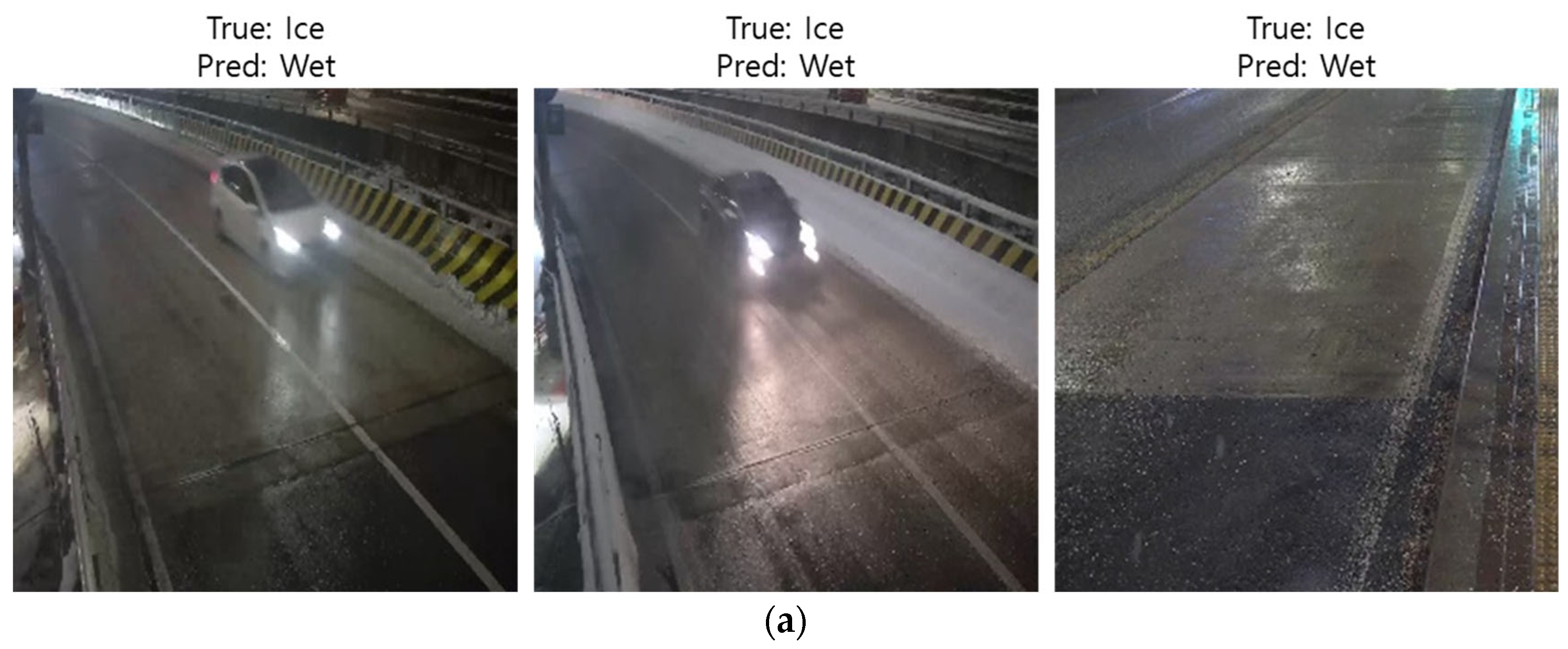
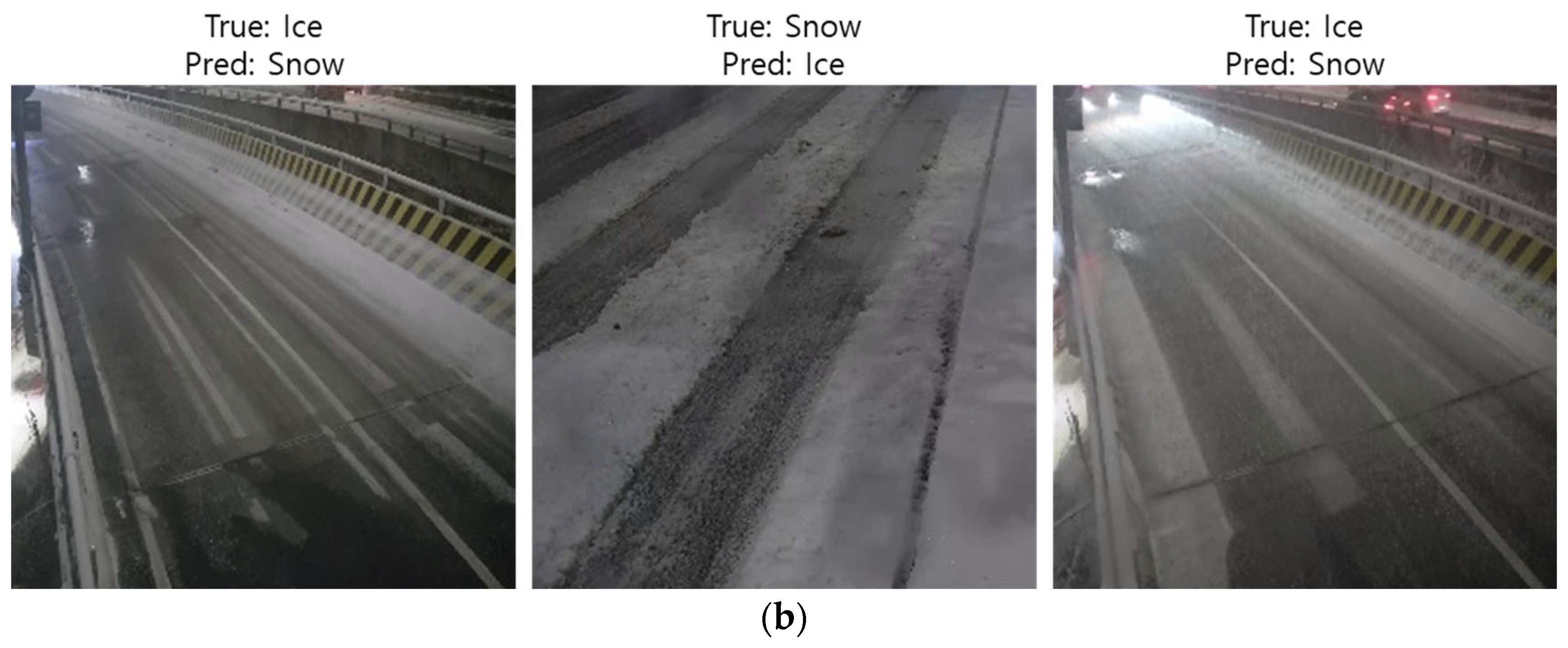
Prediction errors were reviewed for each model. For the model trained on the first database, only 1 error occurred out of 80 cases in the normal class, and only 1 error out of 568 cases in the wet class, indicating excellent accuracy. In contrast, prediction errors occurred more frequently in the slushy conditions. For the ice class, 19 errors were observed out of 530 cases, and for the Snow class, 6 errors out of 503 cases, indicating comparatively lower accuracy. Figure 10 illustrates the prediction errors of the first model for the ice and snow classes. These road surfaces exhibited a mixed distribution of wet, ice, and snow conditions, making it difficult to determine the dominant RSC based on visual inspection. Accordingly, during database construction, such cases were defined as belonging to the most hazardous condition, ice. However, the prediction model classified these images as either wet or snow. As shown in Figure 10a, misclassification between the ice and snow occurs when the visually observed surface moisture indicates that the area covered by ice or snow is greater than that of water. Therefore, regardless of such misclassifications, snow removal operations would still be carried out in practice, and the risk of skidding accidents is relatively low. In contrast, as illustrated in Figure 10b, misclassifying ice as wet may result in incorrect decision-making and delayed snow removal operations.

For the model trained on the second database, no prediction errors occurred in the normal class. In the wet class, two new errors were observed out of 562 cases, both misclassified as ice. In the ice class, 21 errors occurred out of 539 cases, yielding an accuracy similar to that of the first model; however, misclassifications as wet were substantially reduced, while misclassifications as snow markedly increased. For the snow class, 3 errors were observed out of 520 cases, representing a slight improvement in accuracy.

Figure 11 presents the major prediction errors of the second model. The number of cases in which the ice class was misclassified as wet decreased substantially. However, as shown in Figure 11a, some errors persisted when moisture on the road surface reflected light from street lamps or vehicle headlights. Such phenomena were mainly observed in data captured under artificial lighting conditions. Figure 11b shows prediction errors for slushy road surfaces, where water, ice, and snow coexist, indicating that the model tended to classify them as either ice or snow. As with Figure 10a, this type of misclassification is regarded as unlikely to lead to incorrect decision-making in practical contexts.

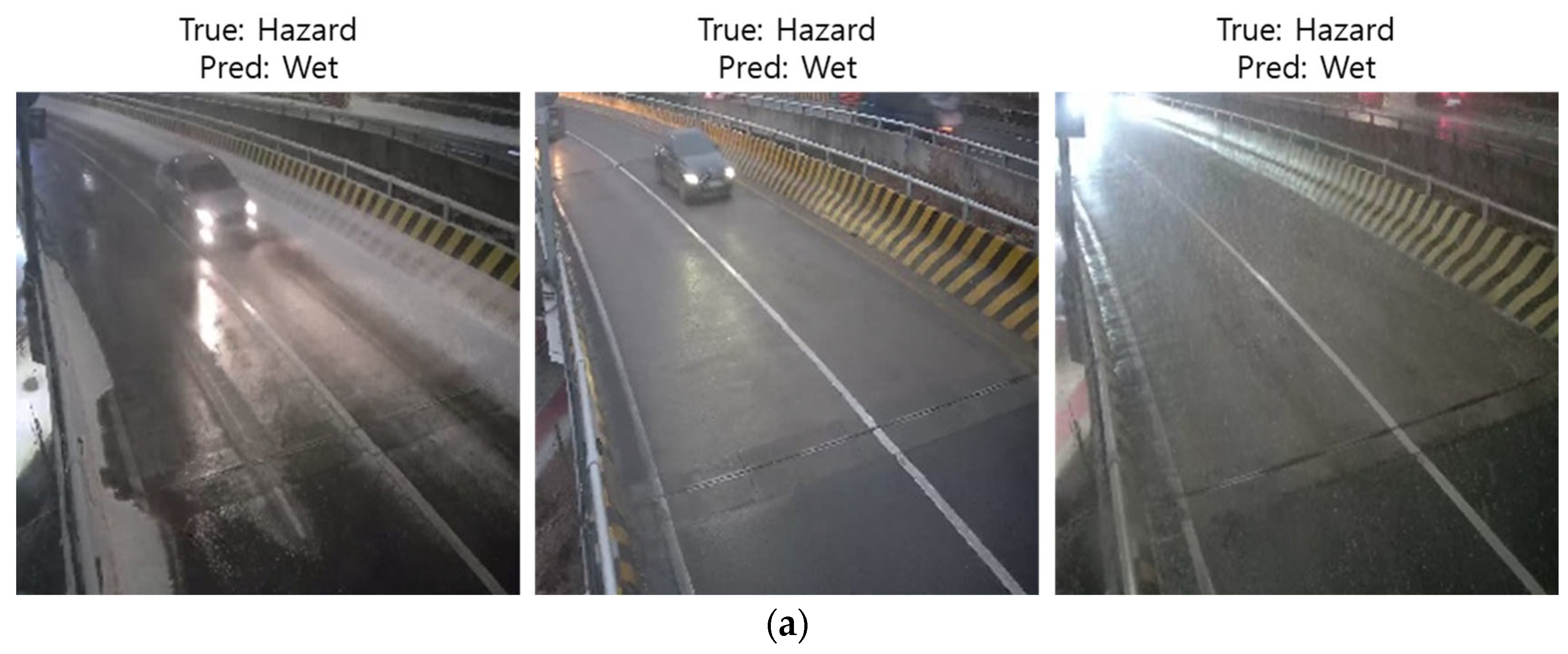
For the model trained with the third database, prediction errors were mainly observed between the wet and hazard classes. No prediction errors occurred in the normal class. In the wet class, 7 errors out of 644 cases were misclassified as hazard, while in the hazard class, 6 errors out of 656 cases were misclassified as wet. Figure 12 presents examples of the misclassified data. Figure 12a shows cases in which the hazard class was misclassified as wet, with some errors attributed to artificial lighting, as in Figure 11a. Meanwhile, Figure 12b illustrates cases where the wet class was misclassified as hazard. Such errors were found to occur when ice and snow on the road had nearly melted, but localized snow was still observed along gutters or adjacent sidewalks. In this study, road surfaces were classified as hazard only when snow was present on the driving lane. However, during the model training process, snow present near gutters was also included in the learning, which likely contributed to these misclassifications. To reduce such errors and enhance model performance, it would be beneficial in the data preprocessing stage to define the target area with a focus on the driving lane or wheel paths, while excluding regions outside the snow removal zone from training data.

Table 7. Summary of Prediction Error Types.

Category	Test Samples	Accuracy	Error Cases	Pavement Type		Artificial Light
				Asphalt	Concrete	Presence	Absence
1st DB	2181	98.76%	27	8	19	3	24
2nd DB	2177	98.76%	27	1	26	7	20
3rd DB	1941	99.28%	14	5	9	6	8

summarizes the types of prediction errors for each model by pavement type and by whether artificial lighting interference was present. In this study, more prediction errors were observed on concrete pavements; however, this result alone is insufficient to conclude that RSC prediction accuracy is lower on concrete surfaces. This is because factors such as snow removal promptness, traffic volume, and snowfall frequency vary across actual field sites. In this study, as shown in Figure 10 through Figure 12, slushy road surfaces were frequently observed at concrete pavements sites. This appears to have contributed to the greater frequency of prediction errors on concrete surfaces. Similarly, the frequency of interference from artificial lighting can vary depending on site-specific factors such as traffic volume (e.g., the frequency of vehicle headlights) and streetlight density. Therefore, based on the summary in Table 7, it is not appropriate to conclude that prediction errors were fewer in cases involving artificial lighting interference. However, during the model development stage, stricter outlier removal should be applied in the preprocessing phase to ensure that artificial lighting interference does not adversely affect model training. Furthermore, when applying the model in practice, it is advisable to avoid predicting RSCs using images captured during vehicles are passage.

Through the analysis of prediction errors, practical issues such as data imbalance and outliers were identified at certain sites. Nevertheless, all models achieved an overall accuracy exceeding 98%, demonstrating strong performance. In particular, the third model achieved the highest accuracy and posed the lowest risk of decision-making errors. From the perspective of road managers, the model trained on the third database is considered the most applicable.

5. Performance Comparison with Pre-Trained Models

In this study, publicly available ImageNet-based model architectures were referenced and fine-tuned using the dataset developed for this research. This approach allowed us to compare the performance of the proposed model with that of pre-trained models. The models selected for comparison were DenseNet-169 [20], Inception-v3 [18], and VGG16 [16].

Table 8. Summary of Comparative Models.

No.	Model	Parameters	Layers
1	Proposed Model (3rd DB)	836,275	17
2	Inception-v3	25,343,027	318
3	VGG16	16,288,851	26
4	DenseNet169	17,755,987	602

presents a comparison of the layer structures and parameter counts between the third RSC prediction model developed in this study and the selected pre-trained models. Overall, the ImageNet-based models were much deeper and had significantly more parameters than the model developed in this study.

Each comparative model was retrained using the dataset from this study, and its performance was compared with that of the proposed model. For the DenseNet-169, Inception-v3, and VGG16 models, the retraining range was set to the bottom 15% of the feature extraction layers. The learning rate was fixed at 0.001, consistent with the setting used in this study.

After fine-tuning, the results of model training were compared as summarized in

Table 9. Training Results of Comparative Models.

No.	Model	Tunning Method	Train_Loss	Val_Loss	Train_Acc	Val_Acc
1	Proposed Model (3rd DB)	-	0.0581	0.0263	98.00%	99.06%
2	Inception-v3	15% Layers	0.1291	0.0793	96.84%	99.06%
3	VGG16	15% Layers	0.0275	0.0430	99.24%	99.38%
4	DenseNet169	15% Layers	0.1998	0.0546	90.20%	99.38%

. All four models achieved very high accuracy on the validation set. The validation loss was lowest for the model developed in this study, whereas the Inception-v3 model showed the highest loss. The DenseNet-169 model exhibited a relatively larger deviation between training and validation accuracy.

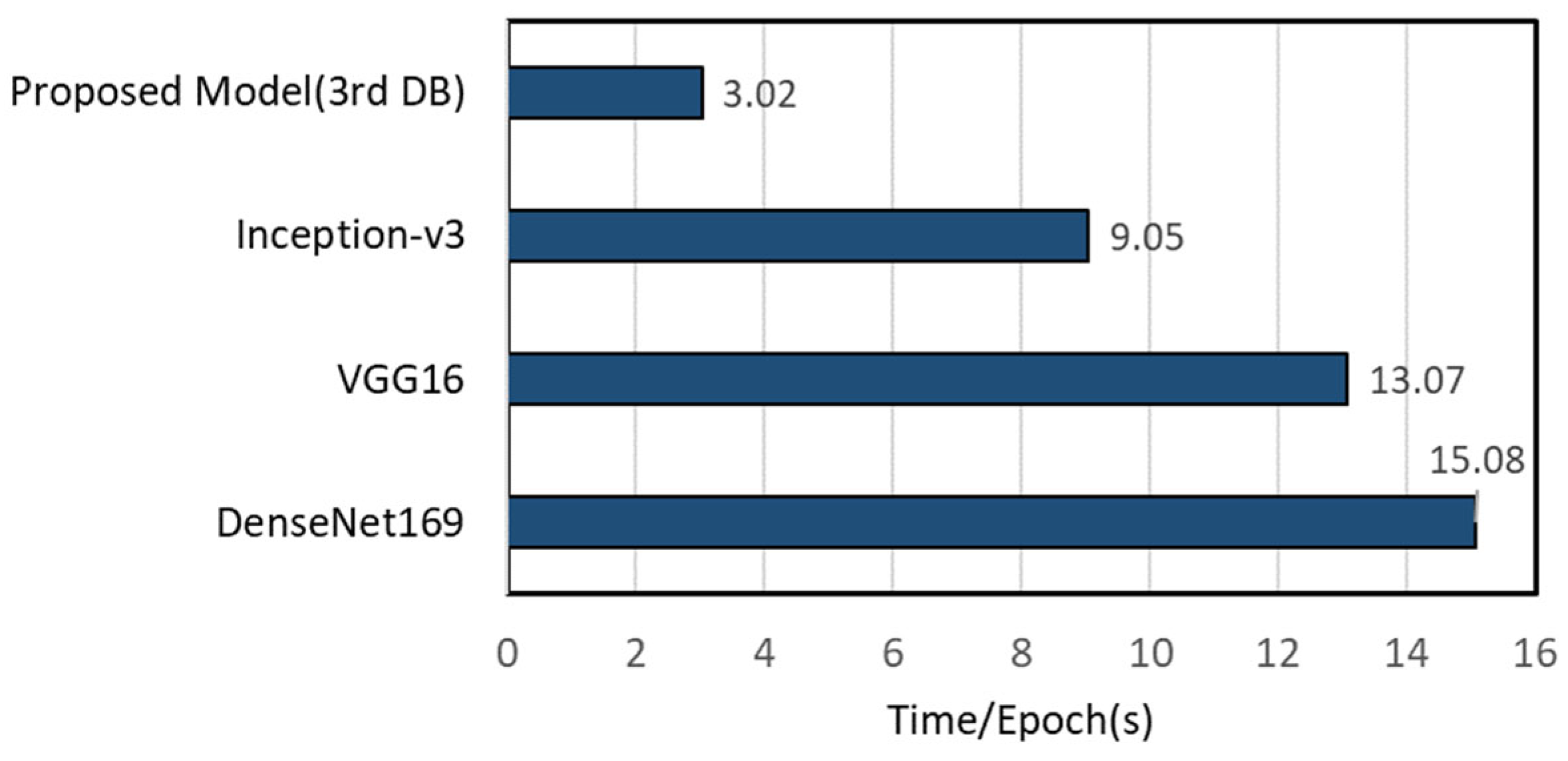
Figure 13 presents the training time per epoch for each comparative model. For all models, a batch size of 32 and a learning rate of 0.001 were applied. Using TensorFlow 2.10.0 and an RTX 4070Ti GPU, the proposed model achieved the fastest training speed, requiring approximately 3 s per epoch. In contrast, Inception-v3, VGG16, and DenseNet-169 took approximately three, four, and five times as long as the proposed model, respectively. In terms of training efficiency relative to accuracy, the proposed model demonstrated the best balance between accuracy and training time. This finding suggests that, in applications such as RSC prediction, where the number of target classes is limited, designing an excessively complex model may not be advantageous from the standpoint of training efficiency.

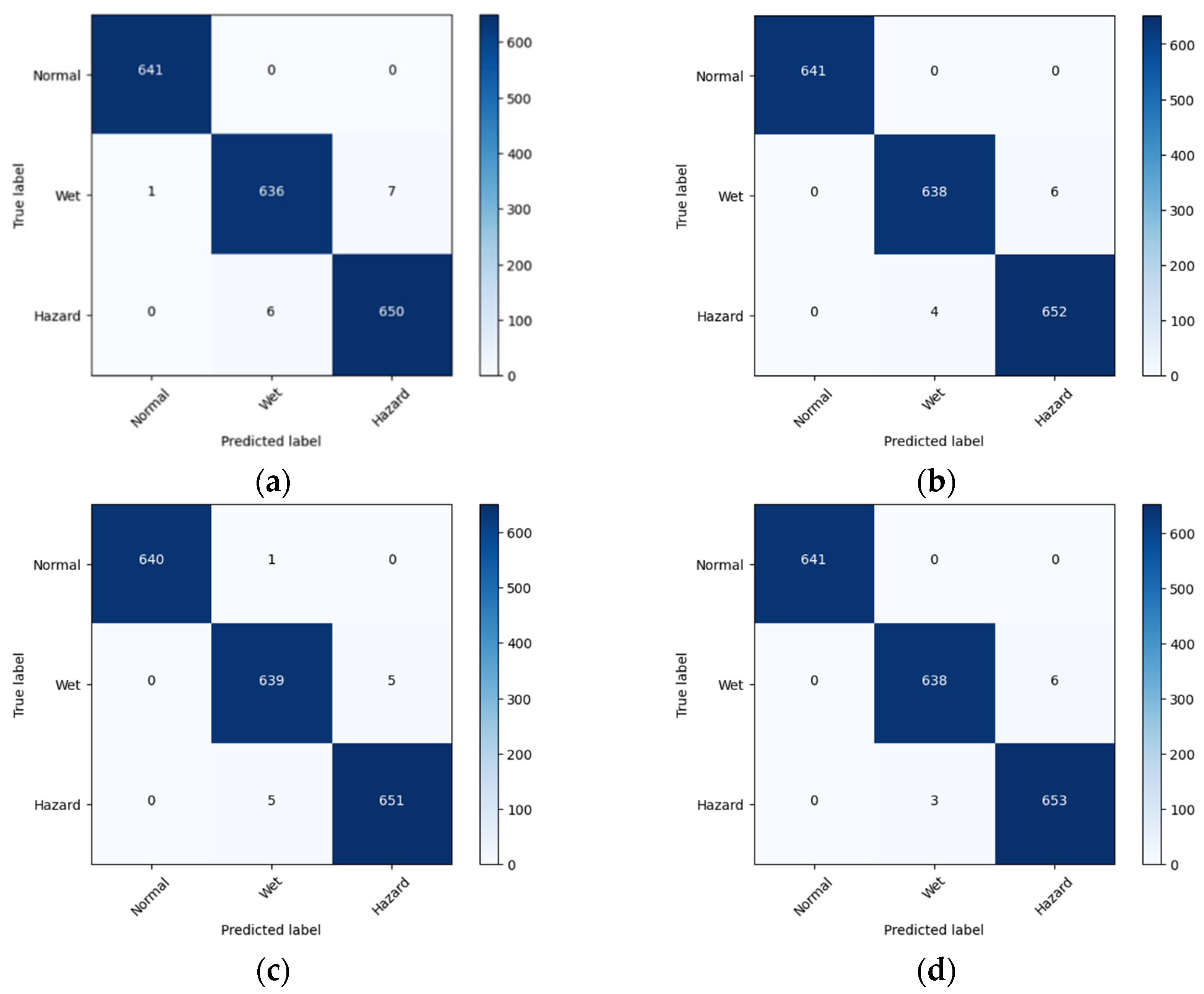
To compare model performance, confusion matrices for the test set are presented in Figure 14 and

Table 10. Performance Evaluation of Comparative Models.

Category	RSC	Precision	Recall	F1-Score
Proposed Model (3rd DB)	Normal	1.00	1.00	1.00
	Wet	0.99	0.99	0.99
	Hazard	0.99	0.99	0.99
Inception-v3 (15% tuning)	Normal	1.00	1.00	1.00
	Wet	0.99	0.99	0.99
	Hazard	0.99	0.99	0.99
VGG16 (15% tuning)	Normal	1.00	1.00	1.00
	Wet	0.99	0.99	0.99
	Hazard	0.99	0.99	0.99
DenseNet169 (15% tuning)	Normal	1.00	1.00	1.00
	Wet	1.00	0.99	0.99
	Hazard	0.99	1.00	0.99

. All models achieved high accuracy on the test set and demonstrated comparable levels of predictive performance.

Ultimately, taking into account the application domain, predictive performance, computational cost and training time, and model complexity from the perspective of road managers, the model developed in this study is considered the most appropriate. This is because it combines a simple structure and fewer parameters with predictive performance nearly equivalent to that of pre-trained models.

6. Discussion

Analysis of the collected data revealed that meteorological events such as snowfall were observed intermittently. Therefore, to prevent class imbalance, it is necessary to sufficiently extend the data collection period in order to secure more minority-class samples. In this study, images were collected from five sites; however, future research would benefit from installing cameras at a wider range of locations to account for variables such as snow removal levels, traffic volume, snowfall intensity, pavement materials, and day/night conditions. It was also identified that the data preprocessing phase needs to be more rigorous. In this study, as shown in Figure 4, all images captured over a 10-s period were transmitted to the server. As illustrated in Figure 5, the data were manually inspected to remove outliers. At this phase, images containing obstacles such as vehicles or pedestrians were primarily removed. However, it was also found that interference from artificial lighting could lead to misclassifications. In practice, it is rare to obtain images entirely free from lighting interference. Nevertheless, to improve the quality of training and testing, it was suggested that images with excessive artificial lighting interference should be rigorously removed in advance.

The first database classified each image based on the condition occupying the largest surface area. In other words, for slushy surfaces where multiple moisture forms coexist, the classification was determined by the dominant form—wet, ice, or snow. While the first model developed using this approach generally achieved accurate classification of the test data, most prediction errors were concentrated in cases where ice surfaces were misclassified as wet. From the perspective of road managers responsible for ensuring timely removal of slip hazards, this type of misclassification constitutes the most critical prediction error. Therefore, the first database was deemed unsuitable for use in developing an RSC prediction model.

The second database followed a similar classification criterion to the first, but with slushy surfaces categorized only as either ice or snow. Since pure ice conditions were rarely observed, most of the prediction errors—similar to those in the first database—occurred during the classification of the ice class. However, in the case of the second database, misclassifications of the ice class as wet were significantly reduced, while misclassifications as snow increased notably. From the perspective of road managers, both the ice and snow classes require prompt snow removal operations. Therefore, misclassifying ice as snow has minimal impact on decision-making outcomes. Accordingly, the second database can be considered more suitable than the first for use in preventing skidding accidents.

The third database was constructed by combining the ice and snow classes into a single hazard class, as both conditions require the same operational response from road managers. Consequently, slushy surfaces—which had been a major source of misclassification in previous models—were also grouped into the hazard class. The model trained using this database demonstrated the highest prediction accuracy among the three models and was deemed the most suitable for supporting road management decision-making.

Although it was initially expected that combining ice and snow into a single class would degrade performance during the feature extraction stage, since these two conditions have distinct visual characteristics and the CNN algorithm extracts features using RGB channels, the training results showed the opposite trend. This is because during database construction, only road surfaces with moisture but without ice or snow were classified as wet. Accordingly, the trained model appears to have predicted the hazard class whenever even small amounts of ice or snow were present in the image. However, to further improve prediction reliability, it is advisable to exclude areas outside the roadway from the target so that residual snow on sidewalks or gutters is not included in the training process.

Using the third database, three pre-trained models were compared with the model developed in this study. In terms of prediction accuracy, all models demonstrated comparable levels of performance, suggesting that pre-trained models are also applicable to RSC prediction. However, because the pre-trained models examined in this study use deep and complex architectures, the lightweight model is considered more suitable for computational efficiency and rapid decision-making.

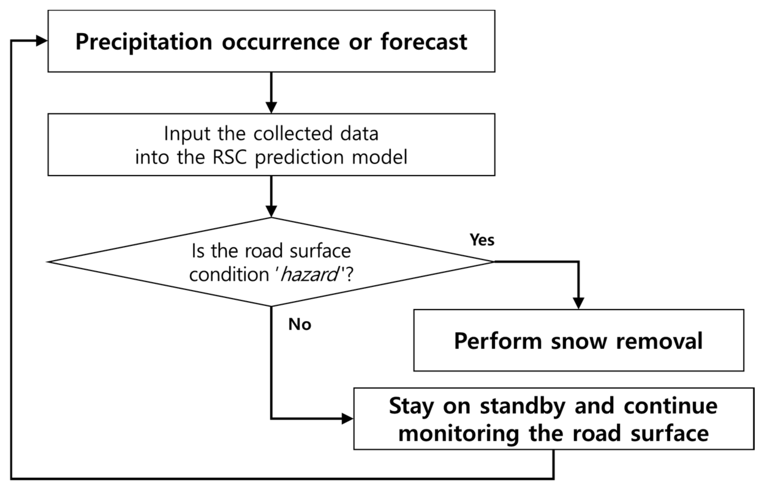
Based on these findings, a snow removal decision-making scenario can be structured as shown in Figure 15. When precipitation occurs or is forecasted, road maintenance personnel monitor the road surface through CCTV cameras installed along the roadside. At this stage, the model developed in this study enables real-time RSC prediction. If the model predicts the RSCs as hazard, the personnel immediately initiate snow removal operations. If the prediction result is normal or wet, the personnel remain on standby while continuing to monitor the road surface. Although such a snow removal decision-making process is possible without the RSC prediction model, it is practically difficult to continuously monitor an extensive road network with limited manpower. The model developed in this study is therefore expected to facilitate the establishment of a sustainable monitoring system and support prompt decision-making, even with constrained human and material resources.

7. Conclusions

Skidding accidents caused by extreme cold weather, sudden heavy snowfall, and road surface freezing have remained a persistent issue. The challenge of overcoming such disasters has been attributed to the excessively vast road networks relative to the limited personnel and resources available for their management. From the perspective of road managers, this study aimed to develop a model capable of automatically predicting RSCs and applicable to extensive road networks to support sustainable snow-removal decision-making. Image data were collected using roadside CCTV cameras, and a lightweight RSC prediction model was developed based on a simple hierarchical structure. In addition, the model’s performance and its major prediction errors were analyzed comparatively according to the class definition methods applied to the collected data.

The most appropriate class definition for supporting practitioner decision-making was determined to be the integration of ice, snow, and slushy conditions into a single class. In addition, the RSC prediction model developed in this study demonstrated predictive performance comparable to that of pre-trained models, while offering greater advantages in terms of computational efficiency. Therefore, from the perspective of road managers for whom real-time RSC assessment is critical, the lightweight model developed in this study is considered suitable for practical application.

Based on this study’s methodology, it is expected that applying the model to a wider range of sites and training it under more diverse data conditions will further advance its predictive capability. The developed prediction model can support timely decision-making for snow removal operations. Through this approach, it is anticipated that the model will reduce disaster risks such as multi-vehicle crashes and associated casualties. In addition, it can enhance disaster resilience by facilitating the prompt restoration of traffic systems.

References

1. Norrman, J.; Eriksson, M.; Lindqvist, S. Relationships between road slipperiness, traffic accident risk and winter road maintenance activity. Clim. Res. 2000, 15, 185–193. [Google Scholar] [CrossRef]
2. Jonsson, P.; Casselgren, J.; Thörnberg, B. Road surface status classification using spectral analysis of NIR camera images. IEEE Sens. J. 2014, 15, 1641–1656. [Google Scholar] [CrossRef]
3. Weng, J.; Liu, L.; Rong, J. Impacts of snowy weather conditions on expressway traffic flow characteristics. Discret. Dyn. Nat. Soc. 2013, 2013, 791743. [Google Scholar] [CrossRef]
4. Call, D.A.; Wilson, C.S.; Shourd, K.N. Hazardous weather conditions and multiple-vehicle chain-reaction crashes in the United States. Meteorol. Appl. 2018, 25, 466–471. [Google Scholar] [CrossRef]
5. Park, M.S.; Kang, M.; Kim, S.H.; Jung, H.C.; Jang, S.B.; You, D.G.; Ryu, S.H. Estimation of road sections vulnerable to black ice using road surface temperatures obtained by a mobile road weather observation vehicle. Atmosphere 2021, 31, 525–537. [Google Scholar] [CrossRef]
6. Kim, H.W.; Choi, M.G.; Kim, S.H.; Kim, B.J.; Baek, S.B.; Jeong, J.H. Statistical analysis of meteorological factors affecting road icing accidents. Int. J. Highw. Eng. 2023, 25, 153–160. [Google Scholar] [CrossRef]
7. Pan, G.; Muresan, M.; Yu, R.; Fu, L. Real-time winter road surface condition monitoring using an improved residual CNN. Can. J. Civ. Eng. 2021, 48, 1215–1222. [Google Scholar] [CrossRef]
8. Kwon, T.J.; Fu, L.; Jiang, C. Road weather information system stations—Where and how many to install: A cost benefit analysis approach. Can. J. Civ. Eng. 2015, 42, 57–66. [Google Scholar] [CrossRef]
9. Takasaki, Y.; Saldana, M.; Ito, J.; Sano, K. Development of a method for estimating road surface condition in winter using random forest. Asian Transp. Stud. 2022, 8, 100077. [Google Scholar] [CrossRef]
10. Crevier, L.P.; Delage, Y. METRo: A new model for road-condition forecasting in Canada. J. Appl. Meteorol. 2001, 40, 2026–2037. [Google Scholar] [CrossRef]
11. Lee, M.; Kim, Y.; Jun, Y.; Yong, H. Prediction of road surface state caused by weather condition using machine learning model. J. Inf. Technol. Archit. 2018, 15, 521–536. [Google Scholar] [CrossRef]
12. Russakovsky, O.; Deng, J.; Su, H.; Krause, J.; Satheesh, S.; Ma, S.; Huang, Z.; Karpathy, A.; Khosla, A.; Bernstein, M.; et al. ImageNet Large Scale Visual Recognition Challenge. Int. J. Comput. Vis. 2015, 115, 211–252. [Google Scholar] [CrossRef]
13. Pratt, L.Y. Discriminability-based transfer between neural networks. In Advances in Neural Information Processing Systems 5 (NIPS 1992); Hanson, S.J., Cowan, J.D., Giles, C.L., Eds.; Morgan Kaufmann: San Mateo, CA, USA, 1993; pp. 204–211. Available online: https://proceedings.neurips.cc/paper/1992/hash/67e103b0761e60683e83c559be18d40c-Abstract.html (accessed on 15 August 2025).
14. Hussain, M.; Bird, J.J.; Faria, D.R. A Study on CNN Transfer Learning for Image Classification. In Proceedings of the UK Workshop on Computational Intelligence (UKCI 2018), Nottingham, UK, 5–7 September 2018; Springer: Cham, Switzerland, 2018; pp. 191–202. [Google Scholar] [CrossRef]
15. Krizhevsky, A.; Sutskever, I.; Hinton, G.E. ImageNet Classification with Deep Convolutional Neural Networks. Commun. ACM 2017, 60, 84–90. [Google Scholar] [CrossRef]
16. Simonyan, K.; Zisserman, A. Very Deep Convolutional Networks for Large-Scale Image Recognition. In Proceedings of the International Conference on Learning Representations (ICLR 2015), San Diego, CA, USA, 7–9 May 2015; Available online: https://arxiv.org/abs/1409.1556 (accessed on 15 August 2025).
17. Chollet, F. Xception: Deep Learning with Depthwise Separable Convolutions. In Proceedings of the IEEE Conference on Computer Vision and Pattern Recognition (CVPR 2017), Honolulu, HI, USA, 21–26 July 2017; pp. 1251–1258. [Google Scholar] [CrossRef]
18. Szegedy, C.; Vanhoucke, V.; Ioffe, S.; Shlens, J.; Wojna, Z. Rethinking the Inception Architecture for Computer Vision. In Proceedings of the IEEE Conference on Computer Vision and Pattern Recognition (CVPR 2016), Las Vegas, NV, USA, 27–30 June 2016; pp. 2818–2826. [Google Scholar] [CrossRef]
19. He, K.; Zhang, X.; Ren, S.; Sun, J. Identity Mappings in Deep Residual Networks. Lect. Notes Comput. Sci. 2016, 9908, 630–645. [Google Scholar] [CrossRef]
20. Huang, G.; Liu, Z.; Van Der Maaten, L.; Weinberger, K.Q. Densely Connected Convolutional Networks. In Proceedings of the IEEE Conference on Computer Vision and Pattern Recognition (CVPR 2017), Honolulu, HI, USA, 21–26 July 2017; pp. 2261–2269. [Google Scholar] [CrossRef]
21. Sandler, M.; Howard, A.; Zhu, M.; Zhmoginov, A.; Chen, L.C. MobileNetV2: Inverted Residuals and Linear Bottlenecks. In Proceedings of the IEEE Conference on Computer Vision and Pattern Recognition (CVPR 2018), Salt Lake City, UT, USA, 18–22 June 2018; pp. 4510–4520. [Google Scholar] [CrossRef]
22. Bianco, S.; Cadene, R.; Celona, L.; Schettini, R. Benchmark analysis of representative deep neural network architectures. IEEE Access 2018, 6, 64270–64277. [Google Scholar] [CrossRef]
23. Lee, H.; Kang, M.; Song, J.; Hwang, K. The Detection of Black Ice Accidents for Preventative Automated Vehicles Using Convolutional Neural Networks. Electronics 2020, 9, 2178. [Google Scholar] [CrossRef]
24. Zhang, C.; Nateghinia, E.; Miranda-Moreno, L.F.; Sun, L. Winter road surface condition classification using convolutional neural network (CNN): Visible light and thermal image fusion. Can. J. Civ. Eng. 2022, 49, 569–578. [Google Scholar] [CrossRef]
25. Pan, G.; Fu, L.; Yu, R.; Muresan, M.I. Winter Road Surface Condition Recognition Using a Pre-Trained Deep Convolutional Neural Network. In Proceedings of the Transportation Research Board 97th Annual Meeting, Washington, DC, USA, 7–11 January 2018; Paper No. 18-00838. Available online: https://trid.trb.org/View/1494597 (accessed on 15 August 2025).
26. Glorot, X.; Bengio, Y. Understanding the Difficulty of Training Deep Feedforward Neural Networks. In Proceedings of the 13th International Conference on Artificial Intelligence and Statistics (AISTATS), Sardinia, Italy, 13–15 May 2010; pp. 249–256. Available online: https://proceedings.mlr.press/v9/glorot10a.html (accessed on 15 August 2025).
27. LeCun, Y.; Bengio, Y.; Hinton, G. Deep learning. Nature 2015, 521, 436–444. [Google Scholar] [CrossRef]
28. Grabowski, D.; Czyżewski, A. System for monitoring road slippery based on CCTV cameras and convolutional neural networks. J. Intell. Inf. Syst. 2020, 55, 521–534. [Google Scholar] [CrossRef]
29. Hashemi, M. Enlarging Smaller Images before Inputting into Convolutional Neural Network: Zero-Padding vs. Interpolation. J. Big Data 2019, 6, 26. [Google Scholar] [CrossRef]
30. Scherer, D.; Müller, A.; Behnke, S. Evaluation of Pooling Operations in Convolutional Architectures for Object Recognition. Lect. Notes Comput. Sci. 2010, 6354, 92–101. [Google Scholar] [CrossRef]
Figure 1. Research Methodology.
Sustainability 17 08794 g001
Figure 2. View of Data Collection Sites and Cameras: (a) Asphalt-1; (b) Asphalt-2; (c) Asphalt-3; (d) Concrete-1; (e) Concrete-2.
Sustainability 17 08794 g002
Figure 3. Video Data Collection Server.
Sustainability 17 08794 g003
Figure 4. Removed Outliers: (a) Examples Included in the Database; (b) Examples Included in the Database; (c) Examples Excluded from the Database.
Sustainability 17 08794 g004
Figure 5. Data Preprocessing: (a) Raw Data and Target Area; (b) Cropped and Resized Data.
Sustainability 17 08794 g005
Figure 6. Five Classes of Road Surface Conditions (RSCs): (a) Normal; (b) Wet; (c) Ice; (d) Snow; (e) Slushy.
Sustainability 17 08794 g006aSustainability 17 08794 g006b
Figure 7. Model Architecture.
Sustainability 17 08794 g007
Figure 8. Loss and Accuracy of CNN Models by Databases: (a) 1st DB; (b) 2nd DB; (c) 3rd DB.
Sustainability 17 08794 g008
Figure 9. Comparison of Confusion Matrix of Models: (a) 1st DB; (b) 2nd DB; (c) 3rd DB.
Sustainability 17 08794 g009
Figure 10. Prediction Error of Model Trained by 1st DB: (a) Mutual Misclassification between Ice and Snow Classes; (b) Misclassification of Ice as Wet.
Sustainability 17 08794 g010aSustainability 17 08794 g010b
Figure 11. Prediction Error of Model Trained by 2nd DB: (a) Misclassification Caused by Artificial Lighting; (b) Misclassification for Slushy Road Surface.
Sustainability 17 08794 g011aSustainability 17 08794 g011b
Figure 12. Predic. on Error of Model Trained by 3rd DB: (a) Misclassification of Hazard as Wet; (b) Misclassification of Wet as Hazard.
Sustainability 17 08794 g012aSustainability 17 08794 g012b
Figure 13. Training Time per Epoch for Comparative Models.
Sustainability 17 08794 g013
Figure 14. Comparison of Confusion Matrix of Models: (a) Proposed Model; (b) Inception-v3; (c) VGG16; (d) DenseNet169.
Sustainability 17 08794 g014
Figure 15. Example of a Snow Removal Decision-Making Scenario.
Sustainability 17 08794 g015