An ISAO-DBCNN-BiLSTM Model for Sustainable Furnace Temperature Optimization in Municipal Solid Waste Incineration

Abstract

With increasing urbanization and population growth, the volume of municipal solid waste (MSW) continues to rise. Efficient and environmentally responsible waste processing has become a core issue in sustainable development. Incineration plays a key role in reducing landfill usage and recovering energy from waste, contributing to circular economy initiatives. However, fluctuations in furnace temperature significantly affect combustion efficiency and emissions, undermining the environmental benefits of incineration. To address these challenges under dynamic operational conditions, this paper proposes a hybrid model combining an Improved Snow Ablation Optimizer (ISAO), Dual-Branch Convolutional Neural Network (DBCNN), and Bidirectional Long Short-Term Memory (BiLSTM). The model extracts dynamic features from control and condition variables and incorporates time series characteristics for accurate temperature prediction, thereby enhancing the overall efficiency of the incineration process. ISAO integrates Lévy flight, differential mutation, and elitism strategies to optimize parameters, contributing to better energy recovery and reduced emissions. Experimental results on real MSWI data demonstrate that the proposed method achieves high prediction accuracy and adaptability under varying operating conditions, showcasing its robustness and application potential in promoting sustainable waste management practices. By improving combustion efficiency and minimizing environmental impact, this model aligns with global sustainability goals, supporting a more efficient, eco-friendly waste-to-energy process.

1. Introduction

With the acceleration of global urbanization and the continuous growth of population, the generation of municipal solid waste (MSW) is increasing rapidly. Efficient and environmentally friendly management of this waste has become a key issue for promoting sustainable development [1], as it directly impacts both environmental quality and resource conservation. The adoption of effective waste management technologies, such as energy recovery through waste incineration, plays a pivotal role in transitioning to a circular economy and reducing overall carbon footprints. Incineration of MSW is an important resource recovery technology. It not only reduces landfill pressure but also recovers thermal energy, decreasing reliance on fossil fuels and supporting a low-carbon economy [2]. Furthermore, incineration provides a viable solution for waste-to-energy conversion, contributing to renewable energy generation and minimizing waste volume, which aligns with global sustainability goals. In the incineration process, furnace temperature plays a critical role in combustion efficiency, pollutant emissions, and energy recovery. Unpredictable temperature fluctuations often lead to reduced combustion performance and increased environmental pollution [3]. Therefore, establishing an accurate furnace temperature model is essential. By predicting temperature changes in real time, operators can adjust control parameters in advance, ensuring high efficiency and stable operation while maximizing energy recovery and minimizing environmental impact. This provides essential technical support for optimizing MSW incineration and advancing sustainable development.

However, accurate modeling of furnace temperature faces multiple challenges. The composition of municipal solid waste is complex and dynamically changing, leading to highly uncertain and nonlinear temperature fluctuations [4]. Similar challenges have been reported in other waste-to-energy and co-pyrolysis studies [5,6]. In addition, variables such as feeder speed, air flow, and combustion rate vary with operating conditions, further increasing modeling difficulty [7]. The lag in temperature response and the limited accuracy of sensors in high-temperature environments also complicate real-time monitoring. Therefore, accurately capturing and modeling the patterns of temperature variation, especially under dynamic and complex conditions, remains a key challenge in furnace temperature modeling for MSW incineration. Existing research in this field has mainly focused on physical mechanism modeling, data-driven machine learning models, and hybrid modeling approaches.

Physical mechanism modeling methods focus on the combustion characteristics of MSWI in both solid and gas phases. These models are built from various perspectives, including combustion reactions, heat transfer, and airflow. For example, reference [8] developed a temperature model of the combustion chamber based on computational fluid dynamics (CFD). In contrast, reference [9] proposed a dynamic combustion chamber model considering the calorific value of the input waste. Because these models are grounded in real physical processes, they can provide accurate physical explanations. However, since MSWI systems involve strongly coupled multiphase reactions and nonlinear disturbances, these models often require significant simplifications and idealizations in practice, making it difficult to precisely describe the temperature variations during the dynamic combustion process.

With the development of machine learning techniques, researchers have introduced deep learning methods into the modeling of incineration processes, allowing models to automatically capture complex patterns and nonlinear relationships from historical data. For example, reference [10] modeled the furnace temperature of MSWI using randomly configured networks, while reference [11] employed a CNN-LSTM to predict dioxin emissions from MSWI. Swarm intelligence algorithms have shown excellent performance in adaptively optimizing key parameters of deep learning models, effectively improving generalization ability and reducing performance fluctuations. Reference [12] combined adaptive population-based optimization with fuzzy neural networks to develop a hybrid model for modeling NOx emissions from MSWI, whereas reference [13] used the BAS algorithm to optimize support vector machine parameters for predicting the main steam flow in MSWI. Compared with physical mechanism models, data-driven machine learning methods offer greater adaptability and flexibility, enabling models to adjust automatically to different incineration conditions and to handle large-scale, complex datasets.

Although data-driven machine learning methods have achieved some progress in modeling municipal solid waste incineration processes, traditional machine learning approaches are usually trained on static data, neglecting the temporal continuity and causal relationships of temperature variations. As a result, these models exhibit poor adaptability to long-term changes, and their predictive accuracy can drop significantly under drastic or sudden changes in operating conditions. In the incineration process, furnace temperature is influenced not only by waste composition, feeder speed, and air flow, but also exhibits pronounced temporal characteristics. Specifically, temperature variation is a dynamic process with time-dependent behavior, where the current temperature state often has a significant impact on future temperature changes. This temporal feature makes it challenging for conventional machine learning models, especially those that do not fully account for time-series characteristics, to accurately capture the complex dynamic behavior of furnace temperature.

To address these issues, researchers have begun exploring mitigation modeling approaches. For example, reference [14] introduced time-series analysis techniques by combining Complete Ensemble Empirical Mode Decomposition with Adaptive Noise (CEEMDAN) and bidirectional long short-term memory networks (BiLSTM), focusing on temporal data patterns and fully accounting for time dependency and long-term correlations. This approach was applied to model historical NOx variations. Reference [15] incorporated multidimensional input data, such as primary air, secondary air, feeder speed, grate speed, waste calorific value, and bed thickness, to establish prediction models for furnace temperature and flue gas oxygen concentration, thereby covering a broader range of operating conditions. Reference [16] combined mechanistic models with enhanced decision trees to predict dioxin emission concentrations. By integrating multiple sub-models and dynamically adjusting model parameters, these methods reduce reliance on single data sources or assumptions, improving model applicability across different scenarios. Reference [17] introduced intelligent optimization algorithms to adjust parameters in real time, enhancing the robustness and stability of combustion and NOx emission models under complex and variable incineration conditions.

Building on the above background and identified research gaps, this study seeks to address the following research questions:

• Under complex and varying operating conditions, how can the key operational variables most influential to furnace temperature fluctuations be effectively identified?
• Can a data-driven model capture the nonlinear temporal dynamics of furnace temperature while maintaining high prediction accuracy and generalization under varying conditions?
• Does applying the Improved Snow Ablation Optimizer (ISAO) for parameter optimization enhance the robustness and stability of furnace temperature modeling?

Accordingly, the following hypotheses are proposed:

• A combination of mechanistic analysis and Random Forest-based feature importance evaluation can effectively identify the dominant air distribution and feeding regulation variables influencing furnace temperature.
• A hybrid model combining a dual-branch CNN with a BiLSTM can better capture the dynamic evolution of furnace temperature.
• Hyperparameter optimization via the Improved Snow Ablation Optimizer (ISAO) can significantly improve the prediction accuracy and generalization ability of the model under complex operating conditions.

Despite the advancements in both physical and data-driven models, these approaches still face limitations when it comes to handling complex, time-varying operational conditions. Specifically, while physical models offer accuracy under controlled conditions, they often require significant simplifications in practice, which limits their application in dynamic environments. On the other hand, machine learning models, though flexible and adaptable, fail to capture the temporal dynamics and complex interactions in the system.

To bridge these gaps, this study proposes a hybrid model that combines the strengths of multiple advanced techniques, addressing the limitations of both traditional methods and existing data-driven approaches. This study introduces a novel hybrid model that combines ISAO, DBCNN, and BiLSTM to predict furnace temperature under complex and fluctuating operating conditions. While existing research has focused on physical mechanism models or traditional machine learning approaches, these methods often struggle with dynamic environmental conditions. The innovation in our approach lies in its ability to handle both spatial (e.g., air distribution) and temporal (e.g., temperature evolution over time) aspects of the problem. The use of ISAO for parameter optimization further enhances the model’s robustness and adaptability, making it well-suited for real-world applications where incineration conditions can vary significantly.

The main contributions of this study are as follows:

A furnace temperature modeling approach is proposed that accounts for variable operating conditions and captures time-series characteristics. A hybrid model structure combining a dual-branch convolutional neural network (DBCNN) with a bidirectional long short-term memory network (BiLSTM) is constructed. The model extracts local dynamic features of high-frequency air distribution variables and low-frequency material distribution variables separately and integrates temporal information, enhancing its ability to model the nonlinear dynamics of furnace temperature under varying conditions.

The improved Snow Ablation Optimizer (ISAO) is introduced to jointly optimize the key parameters of the furnace temperature model, namely the neuron dropout rate δ and the learning rate η, achieving model self-optimization. Building on the original SAO, Lévy flight, differential evolution, and elitism strategies are integrated to enhance the algorithm’s global search capability and convergence accuracy for complex, high-dimensional, and nonlinear problems, thereby improving the model’s robustness and generalization ability.

Based on actual MSWI operational data, comparative experiments were conducted for the proposed model, with RMSE, MAE, MAPE, and R² used to evaluate its performance. The experimental results show that the ISAO-DBCNN-BiLSTM model achieves superior prediction accuracy and dynamic adaptability under varying operating conditions, confirming the effectiveness and generalization capability of the proposed approach.

The overall structure of this paper is organized as follows: Section 2 analyzes the MSWI process and describes the problem of furnace temperature modeling. Section 3 introduces the ISAO-DBCNN-BiLSTM-based furnace temperature model. Section 4 presents the experimental study and results analysis. Finally, Section 5 concludes the paper and discusses directions for future research.

2. MSWI Process Thermal Characteristics Analysis

2.1. MSWI Process Flow

Municipal solid waste incineration (MSWI) is a thermal treatment system that integrates energy recovery and pollution control. Taking a municipal solid waste incineration plant in Beijing as an example, as shown in Figure 1, the overall process can be divided into five functional parts: the waste storage and transportation system, the waste incineration system, the waste heat boiler system, the steam power generation system, and the flue gas treatment system.

First, the municipal solid waste, after short-term fermentation in the waste pit, is fed into the incinerator through a hopper. Inside the incinerator, the waste, driven by the grate, sequentially undergoes drying, combustion, and burnout stages, transforming into high-temperature flue gas and solid residues. The solid residues are collected in a slag pit by a slag scraper for further handling. The high-temperature flue gas passes through the waste heat boiler system for heat exchange, generating superheated steam that drives the turbine in the steam power generation system. The flue gas is then treated through neutralization, adsorption, and multi-stage dust removal processes in the gas treatment system before being discharged into the atmosphere, meeting emission standards.

During the MSWI process, furnace temperature is mainly measured using multiple thermocouples installed at the main combustion zone and the furnace outlet. However, due to the complex and variable composition of the waste, the furnace environment is often characterized by high temperatures and strong corrosiveness. The temperature measurement devices are therefore constrained by both spatial limitations and material durability, resulting in temperature data that may exhibit certain delays and errors.

The regulation of furnace temperature relies on mechanisms such as feeder speed, grate movement speed, primary and secondary air systems, and auxiliary combustion devices. The control effects of these operational variables exhibit nonlinear and strong coupling characteristics, making it difficult for traditional mechanistic models to describe the complex, time-varying, multivariable, and strongly coupled nonlinear features of the incineration process.

2.2. Thermal Characteristics Analysis of the Incineration Process

2.2.1. Mechanistic Analysis of the Combustion Process

The municipal solid waste incineration (MSWI) process is a complex thermochemical transformation involving multiphase materials, fluid flow, heat transfer, and chemical reactions under coupled and interactive fields. During this process, the furnace temperature exhibits complex nonlinear and strongly coupled relationships with multiple factors and is influenced by variations in operating conditions and fluctuations in calorific value, making it difficult to accurately describe using mechanistic models.

During the typical combustion stages, the combustible components in municipal solid waste mainly consist of chemical elements such as C, H, and O, along with small amounts of impurities including N and S. Under ideal complete combustion conditions, the typical chemical reactions occurring in the furnace are as follows:

$$C+O_2\to C{O}_2,$$

(1)

$$C{H}_4+2O_2\to 2H_{2}O+2C{O}_2,$$

(2)

$$C_x{H}_y{O}_z+\left(1-x{\eta }_c+{\displaystyle \frac{y}{4}}-{\displaystyle \frac{z}{2}}\right)O_2\to x{\eta }_{c}C+x\left(1-{\eta }_c\right)C{O}_2+{\displaystyle \frac{y}{2}}{H}_{2}O,$$

(3)

Here, ${\eta }_c$ represents the fraction of carbon in the volatile matter that is converted to fixed carbon. It can be seen that oxygen supply is a necessary condition for the combustion reactions.

A thermodynamics-based mechanistic model of the furnace temperature is established to describe the process of combustion heat conversion and distribution [18]. The model is expressed in Equations (4) and (5), revealing the composition of heat sources in the furnace from the perspective of thermal balance.

$$T_f={\displaystyle \frac{Q_{in}-Q_{heat}-Q_{solid}-Q_{gas}-Q_{loss}}{u_{\mathit{induce}}{c}_{gas}}}+T_0,$$

(4)

$$Q_{\mathit{in}}{=Q}_{\mathit{ncv}}+Q_{airI}+Q_{air\mathit{II}},$$

(5)

Here, T_f is the furnace temperature calculated by the mechanism model. $Q_{\mathit{in}}$ represents the total input heat, while $Q_{\mathit{heat}}$ denotes the total heat loss. $Q_{\mathit{solid}}$ and $Q_{\mathit{gas}}$ refer to the heat losses caused by incomplete combustion of solids and flue gas, respectively. $Q_{\mathit{gas}}$ stands for the physical heat loss from slag. $u_{\mathit{induce}}$ is the induced draft fan flow rate, and $Q_{\mathit{gas}}$ is the average specific heat capacity of flue gas. T₀ indicates the initial furnace temperature. $Q_{\mathit{ncv}}$ represents the basic low-grade heat received from the waste, while $Q_{\mathit{air}I}$ and $Q_{\mathit{air}\mathit{II}}$ are the heat introduced by primary and secondary air, respectively.

2.2.2. Analysis of Factors Affecting Furnace Temperature

Based on the above combustion process analysis, it can be seen that the furnace temperature is jointly influenced by three key factors: oxygen supply, heat sources, and combustion efficiency. In practice, during the combustion process, the adjustment of furnace temperature relies on regulating operational variables according to the current operating conditions, in order to achieve effective temperature control. The following section further analyzes the influencing factors of furnace temperature.

• High-frequency air distribution variables

• Influence of the Outlet Air Temperature of the Primary Air Heater on Combustion Efficiency

A higher outlet air temperature of the primary air heater can increase the kinetic energy of oxygen molecules, thereby enhancing their reaction efficiency and promoting more complete combustion. As the air temperature rises, the reaction between oxygen and municipal solid waste becomes faster and more thorough, resulting in greater heat release. Conversely, when the primary air temperature is low, the movement of oxygen molecules slows down, which weakens the combustion reaction, reduces combustion efficiency, and makes it difficult to increase the furnace temperature effectively. In addition, low-temperature air entering the furnace may cause temperature fluctuations and unstable combustion conditions, which can negatively affect the precision of furnace temperature control.

• Influence of Biogas Flow Rate in the Drying Section on Heat Supply

As an auxiliary fuel, biogas provides additional heat to the incineration process. When the biogas flow rate in the drying section increases, it can rapidly release heat, which facilitates the drying and combustion of waste inside the furnace. This effect is particularly significant when the waste has a high moisture content. A higher biogas flow accelerates the evaporation of moisture, improves the combustibility and calorific value of the waste, and enhances the completeness of combustion and total heat release. Meanwhile, increasing the biogas flow rate in the drying section helps raise the furnace temperature, especially during the drying stage. Conversely, a low biogas flow rate may slow down moisture evaporation, leading to poor ignition conditions and unstable furnace temperature.

• Influence of Inlet Biogas Pressure on Oxygen Supply

A higher inlet biogas pressure enhances the injection performance of biogas, allowing it to distribute more evenly within the furnace and mix more thoroughly with the oxygen in the air. This thorough mixing ensures stable combustion reactions, improves the efficiency of oxygen supply, and promotes greater heat release, thereby increasing the furnace temperature. Moreover, higher pressure improves the contact between biogas and solid waste, increasing the chances of reactions between oxygen and combustible components, which enhances combustion efficiency. In contrast, if the biogas pressure is too low, the biogas distribution becomes uneven, and the mixing with oxygen is insufficient. As a result, incomplete combustion may occur, reducing heat release and making it difficult to reach the desired furnace temperature.

• Influence of Air Flow Rate at Left2 Grate in the Drying Section on Oxygen Supply

An increase in the air flow rate at the Left2 grate in the drying section provides sufficient oxygen for the drying process of solid waste, thereby enhancing oxygen supply during combustion. An appropriate air flow not only facilitates moisture evaporation from the waste but also delivers more oxygen to support complete combustion reactions, leading to an increase in furnace temperature. Conversely, insufficient air flow may result in inadequate oxygen supply, reduced combustion efficiency, and incomplete combustion of combustible components in the waste, ultimately lowering the furnace temperature. Therefore, adjusting the air flow rate is essential to ensure a stable oxygen supply and improve combustion efficiency.

• Influence of Inlet Air Flow in the Combustion Section on Combustion Efficiency

A sufficient inlet air flow in the combustion section ensures an adequate supply of oxygen, which is essential for supporting complete combustion reactions. An appropriate oxygen supply allows combustible substances in the solid waste to fully react, releasing a large amount of heat and thereby increasing the furnace temperature. However, if the inlet air flow is insufficient, the oxygen supply becomes inadequate. As a result, part of the combustible components may not be fully oxidized, leading to incomplete heat release and lower furnace temperature. Therefore, maintaining a proper air flow rate is critical to achieving a stable furnace temperature and ensuring efficient combustion.

2.

Low-frequency material distribution variables

• Influence of Feeder Speed on Heat Release

The feeder speed directly affects the amount of solid waste fed into the furnace. A higher feeder speed introduces more waste, increasing the availability of combustible materials, which contributes to greater heat release. However, if the feeding rate is too high, the combustion reactions inside the furnace may not be completed in time. This can lead to insufficient oxygen supply, reduced combustion efficiency, and ultimately less heat generation. Therefore, moderately adjusting the feeder speed ensures that enough combustible material is available while avoiding excessive feeding that could limit oxygen availability. This helps maintain stable furnace temperature control.

• Influence of Grate Speed in the Combustion Section on Oxygen Supply and Combustion Efficiency

The grate speed in the combustion section directly affects the contact time between the solid waste and oxygen. A slower grate speed extends the residence time of the waste in the furnace, allowing sufficient interaction with oxygen, which improves combustion efficiency, releases more heat, and promotes an increase in furnace temperature. Conversely, a faster grate speed may shorten the contact time between waste and oxygen, resulting in incomplete combustion, reduced combustion efficiency, and insufficient heat release. This makes it difficult to maintain the furnace temperature at the desired level.

It is evident that the furnace temperature is influenced by several operational variables, such as air distribution and feeding regulation, which affect combustion efficiency, heat release, and oxygen supply. Mechanistic analysis reveals the relationships between these variables and furnace temperature, providing the foundational understanding of the system’s behavior. However, due to the complex interactions and feedback mechanisms among these factors, the relationship is highly nonlinear and difficult to describe accurately with traditional mechanistic models.

In the actual incineration process, variables such as waste composition, calorific value, moisture content, feeder speed, air flow, and fuel type often vary and adjust according to operating conditions. These variations directly or indirectly impact the stability and efficiency of the combustion process, causing fluctuations in furnace temperature. For instance, under high-load conditions, changes in waste input and oxygen supply significantly affect temperature, whereas under low-load conditions, these factors have less impact. The interactions between these variables are time-varying, exhibiting different characteristics at different stages. Additionally, variables like feeder speed and grate speed, which control material transport and flow, influence furnace temperature at low frequencies, while variables such as secondary air heater outlet air temperature and biogas flow regulate combustion at higher frequencies, providing more immediate control.

Given the challenges in accurately modeling the highly dynamic and nonlinear relationships, a data-driven approach is employed to complement the mechanistic analysis. The mechanistic insights guide the feature selection process by identifying the most influential variables, which are then incorporated into the data-driven model. This hybrid approach combines the strengths of physical principles with machine learning techniques to better capture the complex, time-varying dynamics that traditional models fail to address. Specifically, the mechanistic analysis informs the design of the model by selecting relevant features, while the data-driven model is used to predict furnace temperature based on these features. The model’s predictions are further validated through physical constraints and system behavior, ensuring consistency with the established mechanistic understanding.

Thus, the integration of mechanistic insights and data-driven methods enhances the model’s robustness, improving its ability to predict furnace temperature under fluctuating and complex operational conditions.

Specifically, the relationship between furnace temperature and its influencing factors can be expressed by Equation (6) and illustrated in Figure 2. Here, $f(·)$ represents the complex nonlinear relationship between furnace temperature and the influencing factors. U denotes the low-frequency material distribution variables, with U_min ≤ U ≤ U_max${, U}_1,{ U}_2,{ U}_3,{ U}_4{, U}_5$ correspond to the outlet air temperature of the primary air heater, biogas flow rate in the drying section, inlet biogas pressure, air flow rate at left2 grate in the drying section, and inlet air flow in the combustion section, respectively. $\mathsf{\Omega }$ denotes the high-frequency air distribution variables, with ${\mathsf{\Omega }}_{\mathit{min}} \le \mathsf{\Omega } \le { \mathsf{\Omega }}_{\mathit{max}}$. Ω₁ and Ω₂ represent the feeder speed and grate speed in the combustion section, respectively. $\widehat{y_i}$ represents the furnace temperature.

$$\widehat{y}=f(U_1, U_2, U_3, U_4, U_5, {\Omega }_1, {\Omega }_2),$$

(6)

As shown in Figure 3, the adjustment cycles of Feeder speed (Ω₁) and Grate speed in the combustion section (Ω₂) are significantly longer than those of the other five variables, and their effects on the furnace temperature (y) generally exhibit a time delay. Therefore, Feeder speed (Ω₁) and Grate speed (Ω₂) are defined as low-frequency material distribution variables, while the remaining five variables (Outlet air temperature of the primary air heater (U₁), Biogas flow rate in the drying section (U₂), Inlet biogas pressure (U₃), Air flow rate at left2 grate in the drying section (U₄), and Inlet air flow in the combustion section (U₅)), which can rapidly respond to furnace temperature fluctuations, are defined as high-frequency air distribution regulation variables.

3. Furnace Temperature Model Based on ISAO-Optimized DBCNN-BiLSTM

3.1. Modeling Strategy

Considering the time-series characteristics of MSWI furnace temperature data, the Bidirectional Long Short-Term Memory (BiLSTM) network can effectively capture long-term dependencies in sequential data, which aligns well with the dynamic patterns of temperature variation [19]. To address the diversity of operating conditions, the dual-branch convolutional neural network (DBCNN) can process multidimensional inputs through separate branches, enhancing feature extraction under different operating scenarios [20]. Furthermore, the Improved Snow Ablation Optimizer (ISAO) can optimize model parameters, enabling self-optimization and further improving model stability and prediction accuracy under variable operating conditions [21]. Therefore, this study adopts a coordinated approach from three aspects: model architecture, collaborative modeling of heterogeneous variables, and key parameter optimization. A furnace temperature model integrating ISAO with the DBCNN-BiLSTM network is proposed, aiming to enhance the modeling capability of dynamic temperature features under complex combustion conditions.

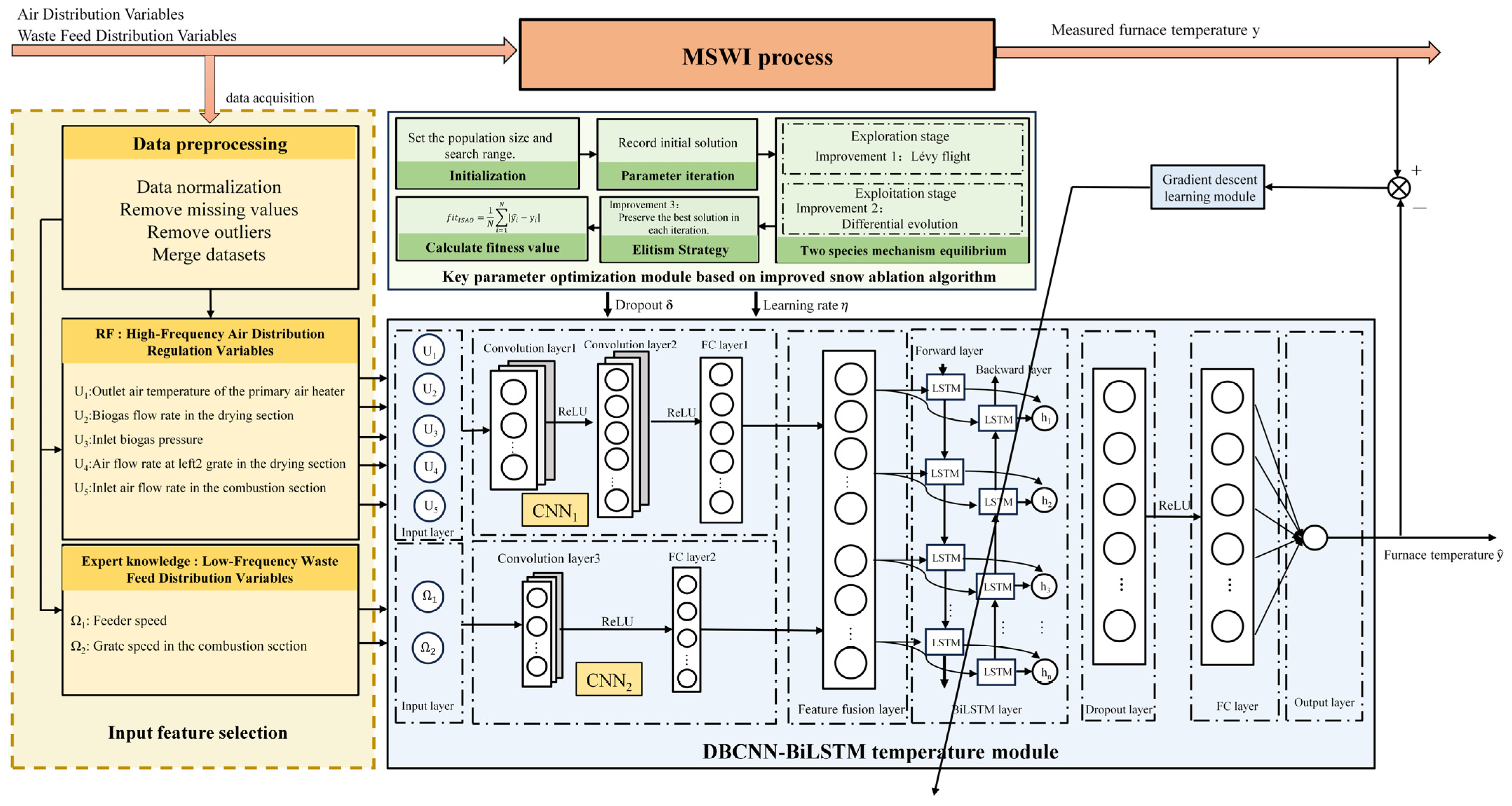
The proposed hybrid model combines three powerful techniques: the Improved Snow Ablation Optimizer (ISAO), Dual-Branch Convolutional Neural Network (DBCNN), and Bidirectional Long Short-Term Memory (BiLSTM). ISAO is introduced for its global search capabilities in complex and high-dimensional optimization tasks, allowing for efficient parameter tuning. The DBCNN architecture is chosen for its ability to simultaneously capture both local dynamic features (air distribution variables) and low-frequency features (material distribution variables). BiLSTM, as a recurrent neural network, excels in modeling temporal dependencies and sequential data, which is critical for accurate prediction of furnace temperature in dynamic environments. The synergy between these methods allows the model to address the nonlinearity, time-series characteristics, and operational variability present in the furnace temperature prediction problem. As shown in Figure 4, the furnace temperature model strategy consists of three main components: the variable selection module, the DBCNN-BiLSTM temperature module, and the key parameter optimization module based on the Improved Snow Ablation Optimizer.

The variable selection module performs data preprocessing and input variable screening. Using the Random Forest algorithm, it evaluates the factors that significantly affect furnace temperature and objectively identifies influential variables from the perspective of data processing.

The subsequent experimental results confirm the consistency with the prior factor analysis. The influencing factors of furnace temperature are also identified as five high-frequency air distribution regulation variables, namely, outlet air temperature of the primary air heater, biogas flow rate in the drying section, inlet biogas pressure, air flow rate at the left2 grate in the drying section, and inlet air flow in the combustion section, along with two low-frequency material distribution variables: feeder speed and grate speed in the combustion section.

The DBCNN-BiLSTM temperature module takes the output of the variable selection module as inputs. Local spatiotemporal features are first extracted through the dual-branch convolutional neural network, followed by feature concatenation and fusion. The fused feature sequence is then fed into the BiLSTM module to capture deeper temporal dependencies, ultimately outputting the furnace temperature.

The ISAO parameter optimization module uses operating condition data (Feeder speed and Grate speed in the combustion section) and applies the improved Snow Ablation Optimizer, incorporating Lévy flight, Differential Evolution, and Elitism Strategy, to optimize and identify the neuron dropout rate ($\delta$) and learning rate ($\eta$).

3.2. Modeling Algorithm

3.2.1. Input Feature Selection

The furnace temperature is influenced by multiple interacting factors, forming a highly complex, nonlinear, and multivariable coupling process. Due to the diverse and intricate physical and chemical reactions involved in the waste incineration process, it is difficult to comprehensively and accurately capture this behavior using traditional mechanism-based models. While the influencing factors of furnace temperature have been previously analyzed from a mechanistic perspective, this section focuses on identifying and selecting the most significant variables from a data-driven viewpoint.

Initially, 23 potentially relevant factors were selected and shown in Appendix A. Random Forest (RF) was used to rank the importance of these variables, and those with higher significance were screened and compared against the results of the earlier mechanism-based analysis. The variables with strong correlations were then retained for subsequent modeling.

Random Forest (RF) is an ensemble learning method composed of multiple decision trees. It exhibits excellent feature selection capability, effectively handles nonlinear relationships among multiple variables, and offers strong resistance to overfitting. RF not only reduces feature dimensionality and computational complexity, but also preserves complex dependencies between variables.

In this study, an RF model consisting of 500 decision trees was constructed. The Out-of-Bag (OOB) error estimation mechanism was used to quantify variable importance.

In the Random Forest model, each tree performs out-of-bag (OOB) prediction. The OOB prediction for sample i is the average of its predictions over all trees where it was OOB:

$${\hat{y}}_i^{\mathit{RF}}={\displaystyle \frac{1}{\left|K_i\right|}}{\displaystyle \sum }_{k\in K_i}{\hat{y}}_i^{\left(k\right),\mathit{RF}},$$

(7)

where ${{\widehat{y}}_i}^{\left(k\right),\mathit{RF}}$ is the prediction by the k-th tree and K_i is the set of trees in which sample i was OOB.

The OOB error evaluates model performance:

$$\mathit{OOB} \mathit{Error} = {\displaystyle \frac{1}{L}}{\displaystyle \sum _{i=1}^L{\left(y_i-{\widehat{y}}_i^{RF}\right)}^2},$$

(8)

Feature importance is computed via the permutation method:

$$I_j = {\displaystyle \frac{1}{\left|K\right|}}{\sum }_{k=1}^{\left|K\right|}\left({\mathit{OOB} \mathit{Error}}_{k ,j} -{\mathit{OOB} \mathit{Error}}_k\right),$$

(9)

Feature importance is computed via the permutation method:

$${\tilde{I}}_j = {\displaystyle \frac{I_j}{{{\displaystyle \sum }}_{m=1}^M{I}_m}},$$

(10)

where OOB Error_k is the baseline OOB error of the k-th tree, ${\mathit{OOB} \mathit{Error}}_{k,j}$ is the OOB error after permuting feature j, L is the total number of samples and M is the total number of features.

To validate the accuracy of the variable importance selected by the RF model, five-fold cross-validation was conducted. In each fold, the feature importance scores obtained from RF were calculated, and the consistency across folds was evaluated using the Spearman rank correlation coefficient:

$$S=1-{\displaystyle \frac{6\Sigma d_i^2}{n\left(n^2-1\right)}},$$

(11)

where d_i represents the rank difference between two rankings, and n is the number of features.

Based on the feature importance ranking obtained from the Random Forest model and validated by five-fold cross-validation and Spearman rank correlation analysis, seven key input variables were ultimately selected. These include Outlet air temperature of the primary air heater (U₁), Biogas flow rate in the drying section (U₂), Inlet biogas pressure (U₃), Air flow rate at left2 grate in the drying section (U₄), Inlet air flow in the combustion section (U₅), Feeder speed (Ω₁), and Grate speed in the combustion section (Ω₂). These seven variables are consistent with the previous feature analysis. The detailed evaluation process is provided in Section 4.2

3.2.2. DBCNN-BiLSTM-Based Furnace Temperature Model

This study adopts a structure combining a Dual-Branch Convolutional Neural Network (DBCNN) and a Bidirectional Long Short-Term Memory (BiLSTM) to improve the accuracy and stability of furnace temperature modeling under varying operating conditions. The DBCNN consists of two parallel convolutional branches, separately processing the high-frequency air distribution regulation variables U and the low-frequency material distribution variables Ω. This design enables the model to maintain global trend modeling capability while capturing and extracting effective information from different scales and types of input combinations, thereby enhancing the dynamic modeling ability of the model. The dual-branch structure has demonstrated superior performance in modeling heterogeneous data across various fields. For example, Reference [22] employed a dual-branch CNN and TCN architecture to forecast solar irradiance. Reference [23] applied a sliding-window approach combined with a dual-branch CNN for synchronous prediction of coal and electricity consumption in the cement forging process.

Long Short-Term Memory (LSTM) networks and their bidirectional variant, BiLSTM, possess the ability to capture long-term dependencies, effectively characterizing the dynamic trends in sequential data. After fusing the convolutional features from the dual branches, the BiLSTM integrates both forward and backward temporal information, making it well-suited for modeling complex nonlinear dynamic processes. This structure can comprehensively capture the intrinsic temporal patterns of furnace temperature, enabling higher-order modeling of sequential dependencies from previous stages. It is particularly effective in identifying temperature trends and capturing temporal features under non-stationary combustion conditions.

Specifically, the high-frequency air distribution variables U and low-frequency material distribution variables Ω serve as inputs to the two separate branches, where U = [U₁, U₂, U₃, U₄, U₅], and Ω = [Ω_1, Ω₂]. Each input channel independently passes through a series of convolutional layers followed by ReLU activation to extract local spatial features.

$$F_1=ReLU\left(W_1^{(2)}\ast ReLU(W_1^{(1)}\ast U+b_1^{(1)})+b_1^{(2)}\right),$$

(12)

$$F_2=ReLU\left(W_2\ast \Omega +b_2\right),$$

(13)

where F₁ and F₂ represent the feature maps of the high-frequency air distribution branch and the low-frequency material distribution branch, respectively, after convolution and activation.; * denotes the convolution operation; $W_1^{(1)}$ and $W_1^{(2)}$ are the convolution kernel weights matrices for the high-frequency air distribution branch (CNN₁), while W₂ is the convolution kernel weight matrix for the low-frequency material distribution branch (CNN₂). Similarly, $b_1^{(1)}$ and $b_1^{(2)}$ are the bias vectors for the convolution layers in CNN₁, and b₂ is the bias vector for the convolution layers in CNN₂.

After passing through their respective convolutional branches, the features from the two branches are fused through a concatenation operation:

$$F=\left[F_1;F_2\right],$$

(14)

F is the concatenated feature vector after merging feature maps from both branches.

The fused feature sequence is then fed into the BiLSTM layer, which consists of LSTM units in both forward and backward directions. The forward and backward LSTM structures process the input sequence in chronological and reverse order, respectively, and can be expressed as follows:

$$\overrightarrow{h_{\tau }}=LST{M}_{forward}\left(x_{\tau },h_{\tau -1}\right),$$

(15)

$$\overleftarrow{h_{\tau }}=LST{M}_{backward}\left(x_{\tau },h_{\tau +1}\right),$$

(16)

$$H_{\tau }=\left[\overrightarrow{h_{\tau }}+\overleftarrow{h_{\tau }}\right],$$

(17)

where $\overrightarrow{h_{\tau }}$ and $\overleftarrow{h_{\tau }}$ are the forward and backward LSTM outputs, respectively; $H_{\tau }$ is their concatenated representation.

The BiLSTM output $H_{\tau }$ is first processed through a fully connected (FC) layer with ReLU activation, followed by a Dropout layer to prevent overfitting. Finally, another FC layer maps the features to a scalar output, from which the temperature error is computed and backpropagated for optimization. The final output is the predicted furnace temperature.

$${\widehat{y}}_{\tau }=W_o\cdot Dropout\left(ReLU\left(W_f{H}_{\tau }+b_f\right)\right)+b_o,$$

(18)

where $W_f$ and $b_f$ are the weight matrix and bias term of the fully connected layer, $W_o$ and $b_o$ are the weight matrix and bias term of the output layer, and ${\widehat{y}}_{\tau }$ is the predicted temperature at time step $\tau$.

The model is trained using the Adam optimizer, which, with its adaptive learning rate mechanism, effectively accelerates convergence and enhances robustness. Both the learning rate and dropout rate influence training stability. The learning rate determines the step size for parameter updates: too large may cause oscillation and divergence, while too small slows convergence. The dropout rate randomly deactivates neuron connections to prevent overfitting, but an improper setting can weaken the model’s expressive capacity. Properly configuring these two parameters can significantly improve the stability and accuracy of temperature modeling under complex and varying operating conditions.

3.2.3. Optimization of Dropout Rate and Learning Rate Based on ISAO

In modeling the furnace temperature of municipal solid waste incinerators, the model performance is highly sensitive to the dropout rate and learning rate, as these parameters directly affect the model’s ability to adapt to time-varying operating conditions and the nonlinearity of the combustion process. Therefore, this study further introduces the Improved Snow Ablation Optimizer (ISAO) to jointly optimize the dropout rate and learning rate of the temperature model. The Snow Ablation Optimizer (SAO) [24] features a simple structure and high search efficiency, but suffers from limited convergence accuracy and a tendency to become trapped in local optima when solving high-dimensional and multimodal optimization problems. SAO has already been effectively applied in model parameter optimization [25,26]. In this study, Lévy flight, Differential Evolution (DE), and the Elitism Strategy are incorporated into the original SAO framework to enhance its global optimization capability in high-dimensional nonlinear parameter tuning.

To improve the accuracy and robustness of the model, this study applies an Improved Snow Ablation Optimizer (ISAO) to optimize the key parameters of the DBCNN-BiLSTM model. The following section provides a detailed explanation of the original SAO algorithm and the enhancement strategies adopted.

Improvements of the SAO Algorithm

The Snow Ablation Optimizer (SAO), proposed by Deng et al. [24], simulates the physical phenomena of snow melting and sublimation in nature and serves as an efficient optimization algorithm. The algorithm incorporates three main strategies: the snow sublimation exploration strategy, the snow melting exploitation strategy, and the dual-population mechanism.

• Snow Sublimation Exploration Strategy

This strategy is inspired by the physical phenomenon of snow sublimation, during which solid snow directly transforms into water vapor. The irregular molecular motion observed in this process is simulated to model stochastic behavior in the search space. In SAO, Brownian motion is used to model the random perturbations of individuals in the search space. This enhances the global exploration capability and prevents premature convergence to local optima.

The strategy enables the algorithm to uniformly cover the entire search space, achieving large-scale exploration. As a result, SAO exhibits a highly dispersed characteristic during global search.

The position update of each individual is calculated as follows:

$$Z_i\left(t+1\right)=Elite\left(t\right)+BMi\left(t\right)\otimes \left\{{\theta }_1\cdot \left[G\left(t\right)-Z_i\left(t\right)+\left(1-{\theta }_1\right)\cdot \left(\overline{Z}\left(t\right)-Z_i\left(t\right)\right)\right]\right\},$$

(19)

$$Elite\left(t\right)\in \left\{G\left(t\right),Z_{second}\left(t\right),Z_{third}\left(t\right),Z_c\left(t\right)\right\},$$

(20)

$$Z_c\left(t\right)={\displaystyle \frac{1}{N_{p1}}}{\displaystyle \sum _{i=1}^{N_{p1}}{Z}_i\left(t\right)},$$

(21)

$$\overline{Z}\left(t\right)={\displaystyle \frac{1}{N_p}}{\displaystyle \sum _{i=1}^{N_p}{Z}_i\left(t\right)},$$

(22)

where t denotes the iteration number, and i represents the index of individuals in the population. $Z_i\left(t\right)$ is the position vector of the i-th individual at iteration t, and $BMi\left(t\right)$ is the Brownian motion-based random vector generated from a Gaussian distribution. The symbol $\otimes$ denotes the Kronecker product, and ${\theta }_1$ is a random number in the range [0, 1]. $G\left(t\right)$ represents the current best solution, while $Elite\left(t\right)$ refers to an individual randomly selected from the top three elites in the population. $Z_c\left(t\right)$ and $\overline{Z}\left(t\right)$ represent the centroid of the top 50% individuals by fitness and the overall population centroid, respectively. $Z_{second}\left(t\right)$ and $Z_{third}\left(t\right)$ are the positions of the second-best and third-best individuals, respectively. N_p is the total number of individuals in the population, and N_p1 is the number of leader individuals, typically half of N_p.

• Snow Melting Exploitation Strategy

This strategy simulates the process in which snow melts into liquid water. By introducing a daily factor, the movement of individuals toward the global optimum is controlled, thereby enhancing the local exploitation capability. This mechanism encourages individuals to converge around the global best solution, improving the algorithm’s local search accuracy.

The position update of each individual is calculated as follows:

$$Z_i\left(t+1\right)=M\cdot G\left(t\right)+B{M}_i\left(t\right)\otimes \left\{{\theta }_2\cdot \left[G\left(t\right)-Z_i\left(t\right)+\left(1-{\theta }_2\right)\cdot \left(\overline{Z}\left(t\right)-Z_i\left(t\right)\right)\right]\right\},$$

(23)

$$M=\left(0.35+0.25\times {\displaystyle \frac{e^{\frac{t}{t_{max}}}-1}{e-1}}\right)\times e^{{\displaystyle \frac{-t}{t_{max}}}},$$

(24)

where θ₂ is a random number in the range [−1, 1]; M is a weighting factor simulating the snow ablation rate; and t_max denotes the maximum number of iterations.

• Dual-Population Mechanism

SAO employs a dual-population parallel cooperative strategy to enhance search capability and diversity. In the early stages of the algorithm, the entire population is randomly divided into two equally sized sub-populations, responsible for exploration and exploitation, respectively. As iterations proceed, the sizes of the two sub-populations are gradually adjusted by increasing the exploration population and reducing the exploitation population. This balance between exploration and exploitation improves the algorithm’s global search ability and local convergence accuracy.

Although the Snow Ablation Optimizer (SAO) demonstrates strong search capability in global optimization problems, its global exploration and local exploitation abilities tend to weaken as iterations increase when the objective function exhibits complex multimodal characteristics. The algorithm lacks an effective mechanism to escape local optima. In later iterations, the convergence rate slows down, and population diversity decreases, which may lead to insufficient search capability. In addition, SAO evaluates the fitness of all individuals at each iteration, resulting in a significant computational cost.

Therefore, to further enhance its global search capability, improve its ability to escape local optima, and increase computational efficiency, the following improvement strategies are introduced.

• Global Jump Exploration Based on Lévy Flight Strategy

Lévy flight is a type of random walk that follows a Lévy distribution, commonly observed in natural phenomena such as foraging behaviors and migration paths. Compared to standard Gaussian perturbations, Lévy distributions exhibit heavy-tailed characteristics, enabling occasional long-distance jumps. This enhances the population’s ability to escape local optima and significantly improves the global exploration capability of the algorithm. In the original SAO algorithm, the exploration phase relies primarily on Gaussian disturbances based on Brownian motion to update positions. However, Gaussian perturbations are relatively concentrated in magnitude and lack the ability to make long jumps, making the population prone to premature convergence. In this study, the Mantegna algorithm is employed to sample the Lévy distribution, generating step sizes with intermittent, high-magnitude perturbations, which are effective in improving the individuals’ jump search capabilities. The corresponding equation is as follows:

$$Lévy = {\displaystyle \frac{u}{{\left|v\right|}^{\frac{1}{\beta }}}},$$

(25)

In the equation, β is the stability parameter of the Lévy distribution. u and v are random variables following a normal distribution, where $u\sim N\left(0,{\sigma }_u^2\right)$ and $v\sim N\left(0,{\sigma }_v^2\right)$. The standard deviation of the normal distribution for v is set as ${\sigma }_v=1$, while the standard deviation ${\sigma }_u$ is calculated using the following formula:

$${\sigma }_u={\left\{{\displaystyle \frac{\Gamma \left(1+\beta \right)sin\left(\pi \beta /2\right)}{\Gamma \left[\left(1+\beta \right)/2\right]\beta 2^{\left(\beta -1\right)/2}}}\right\}}^{1/\beta },$$

(26)

where Γ denotes the Gamma function, and β is set to 1.5.

• Maintaining Population Diversity Based on Differential Evolution

In the exploitation stage, a DE/current-to-best/1 strategy from Differential Evolution (DE) is introduced. By integrating the current individual position, the global best solution direction, and the population’s internal differential information, a directional and diverse perturbation mechanism is constructed to maintain population diversity and drive exploitation. This strategy not only improves the structural quality of the search path but also enhances convergence efficiency and the ability to escape local optima during local exploitation.

For the current individual Z_i(t), its differential mutation candidate solution D_i is generated as follows:

$$D_i=Z_i\left(t\right)+F_d\cdot \left[Z_{best}\left(t\right)-Z_i\left(t\right)\right]+F_d\cdot \left[Z_{j1}\left(t\right)-Z_{j2}\left(t\right)\right],$$

(27)

where Z_best(t) represents the current best individual; Z_j1(t) and Z_j2(t) are two randomly selected distinct individuals from the population such that j₁ ≠ j₂ ≠ i. F_d is the differential scaling factor, which is set to 0.5 in this study.

The candidate solution D_i is subjected to boundary constraints to ensure that it remains within the defined variable domain:

$$D_i=\mathit{min}\left(\mathit{max}\left(D_i,L_b\right),U_b\right),$$

(28)

where L_b and U_b denote the lower and upper bounds of the decision variables, respectively.

The above differential mutation strategy is embedded into the evolution process of the exploitation sub-population. First, each exploitation individual Z_i(t) is updated using the Brownian motion perturbation of the original SAO algorithm to obtain a temporary solution $Z_i^{\mathit{SAO}}(t)$ according to Equation (23). With a probability of p = 0.2, the differential mutation operation is performed to generate the candidate solution D_i according to Equation (28). The fitness of D_i is then compared with that of $Z_i^{\mathit{SAO}}(t)$; if D_i is superior, it replaces the original solution, otherwise the temporary solution is retained. This mechanism preserves the advantage of local convergence while continuously introducing diversity information from the search space, thereby achieving diversity-driven exploitation and significantly enhancing the algorithm’s robustness and stability in global optimization.

• Global Best Preservation Based on the Elitism Strategy

The Elitism Strategy is a mechanism that directly preserves the best individuals during iterative optimization, aiming to ensure the transmission of global best information and prevent high-quality solutions from being destroyed or lost during random updates. In the SAO algorithm, individual position updates rely on stochastic perturbations, which help maintain population diversity but also introduce considerable uncertainty. This uncertainty may cause previously obtained high-quality solutions to be replaced during iterations, thereby affecting stability and convergence performance.

Therefore, the Elitism Strategy is incorporated into the improved SAO algorithm. At the end of each generation, the current best individual $Z_{best}\left(t\right)$ is retained at the end of the next-generation population, ensuring that the global best information is not lost. This enhances the overall stability of the algorithm, accelerates convergence, guarantees a lower bound on solution quality, and fundamentally strengthens the transmission of global best information, thereby increasing the robustness and reliability of global optimization.

Construction of the Objective Function

The joint domain of the dropout rate and learning rate is defined as:

$$\left(\eta ,\delta \right)\in \left[0.0001,0.01\right]\times \left[0.05,0.5\right],$$

(29)

The proposed ISAO optimization algorithm is employed to search for the optimal combination of dropout rate and learning rate for the furnace temperature model.

Table 1. Mapping between the ISAO and Key Parameter Optimization of the Furnace Temperature Model.

ISAO Term	Meaning in Parameter Optimization Task
Snow particle	A candidate solution representing a specific set of model hyperparameters
Snow particle population	The set of all candidate hyperparameter solutions
Snow ablation process	One iteration of the optimization process
Snow field	The solution space defined by the current population
Snow particle movement	The search process for optimal hyperparameters
Melting & migration behavior	The update mechanism for candidate solutions based on exploration and exploitation
Elite snow particles	The set of best-performing solutions preserved to maintain global optimal information

presents the correspondence between the ISAO optimization algorithm and the parameter optimization problem. To evaluate the model performance under different parameter combinations, the mean absolute error (MAE) is used as the fitness function, and the objective function is constructed as follows:

$$fi{t}_{ISAO}={\displaystyle \frac{1}{N}}{\displaystyle \sum _{i=1}^N\left|{\widehat{y}}_i-y_i\right|},$$

(30)

where N is the total number of samples, ${\widehat{y}}_i$ denotes the predicted furnace temperature of the i-th sample under the current set of key parameters, and y_i is the corresponding ground truth furnace temperature.

3.3. Implementation Steps of the Furnace Temperature Model

As shown in Figure 5, the implementation steps of the ISAO-DBCNN-BiLSTM furnace temperature model are as follows:

Step 1: Preprocess the collected data, select model input variables using Random Forest (RF), normalize the data, and split it into training, validation, and test sets.

Step 2: Initialize ISAO parameters by setting the population size and maximum number of iterations, recording initial positions, and calculating the initial fitness values.

Step 3: Compute the adaptive step size based on the current iteration according to Equation (24).

Step 4: Divide the population into Exploration Subpopulation Pa and Exploitation Subpopulation Pb.

Step 5: Update the positions of individuals in the Exploration Subpopulation Pa. If the Lévy flight strategy is triggered, update positions according to Equation (27); otherwise, update according to Equation (19).

Step 6: Update the positions of individuals in the Exploitation Subpopulation Pb. With a probability p = 0.2, trigger the Differential Evolution (DE) strategy. If triggered, update positions according to Equation (28); otherwise, update according to Equation (23).

Step 7: Apply the Elitism Strategy to preserve the current global best individual; check if the maximum number of iterations has been reached. If not, return to Step 3.

Step 8: Once the maximum number of iterations is reached, output the optimized learning rate η and dropout rate δ.

Step 9: Update the DBCNN-BiLSTM model parameters based on the optimization results and compute the furnace temperature.

Step 10: Reverse the normalization of the model outputs to obtain the final furnace temperature.

4. Experimental Study

4.1. Data Description and Model Evaluation Metrics

The experimental data used in this study were collected from the actual operation of a municipal solid waste incineration plant in a city in China. The data were sampled at 1-s intervals, and a total of 13,000 consecutive time-series samples were selected for modeling and analysis. The dataset includes furnace temperature, air flow rate, air pressure, feeder speed, and other variables, which exhibit typical characteristics of dynamic coupling and varying operating conditions.

During data preprocessing, missing values and outliers were first identified. Missing values were filled using linear interpolation based on neighboring time points. Outliers were detected by comparing each sample with the moving average over a short window and removed if they exceeded three standard deviations. Additionally, a Gaussian filter was applied to reduce high-frequency noise.

To improve the training efficiency and stability of the model, all variables were normalized to the range [0, 1].

The normalization was performed using the following formula:

$$x^{*}={\displaystyle \frac{x-x_{\mathit{min}}}{x_{max}-x_{min}}},$$

(31)

where $x$ represents the original data, $x^{*}$ denotes the normalized data, $x_{max}$ and $x_{min}$ indicate the maximum and minimum values of the corresponding variable in the training set, respectively.

To evaluate the generalization ability of the model, the dataset was divided after preprocessing: 70% was used as the training set, 15% as the validation set, and the remaining 15% as the test set. These subsets were used for model training and performance evaluation, respectively.

To comprehensively assess the accuracy and robustness of the temperature prediction model, four commonly used evaluation metrics were employed: Root Mean Square Error (RMSE), Mean Absolute Error (MAE), Mean Absolute Percentage Error (MAPE), and the Coefficient of Determination (R²). The definitions of these metrics are as follows:

$$\mathrm{RMSE}=\sqrt{{\displaystyle \frac{1}{N}}{\displaystyle \sum _{\mathrm{i}=1}^N{\left(y_i-{\widehat{y}}_i\right)}^2}},$$

(32)

$$MAE={\displaystyle \frac{1}{N}}{\displaystyle \sum _{i=1}^N\left|y_i-{\widehat{y}}_i\right|},$$

(33)

$$MAPE={\displaystyle \frac{100\%}{N}}{\displaystyle \sum _{i=1}^N\left|\frac{y_i-{\widehat{y}}_i}{y_i}\right|},$$

(34)

$$R^2=1-{\displaystyle \frac{{\displaystyle \sum _{i=1}^N{\left(y_i-{\widehat{y}}_i\right)}^2}}{{\displaystyle \sum _{i=1}^N{\left(y_i-\overline{y}\right)}^2}}},$$

(35)

where N denotes the number of samples; $y_i, \widehat{y_i}, \overline{y}$ represent the model output of the i-th sample, the true value of the i-th sample, and the mean value of all samples, respectively.

Table 2. Basic Information of Variables.

Symbol	Variable Name	Range	Unit
U1	Outlet air temperature of the primary air heater	175.4872~187.4064	°C
U2	Biogas flow rate in drying section	36.9311~75.9367	m3/h
U3	Inlet biogas pressure	8.6702~9.1871	Kpa
U4	Air flow rate at left2 grate in the drying section	2.1125~3.7085	km3N
U5	Inlet air flow in combustion section	6.4822~11.2061	km3N
Ω1	Feeder speed	20~70	%
Ω2	Grate speed in the combustion section	20~40	%
y	Actual furnace temperature	912.94~983.96	°C

presents the basic information of the input variables used in the model.

4.2. Experimental Assessment of Furnace Temperature Modeling and Optimization

4.2.1. Feature Selection Results

Based on the feature selection approach described in Section 3.2.1, the Random Forest (RF) algorithm was applied to rank the importance of the input variables. As shown in Figure 6, the top eight variables identified by the RF model are biogas flow rate in the drying section, outlet air temperature of the primary air heater, air flow rate at left1 grate in the drying section, inlet biogas pressure, air flow rate at left2 grate in the drying section, air flow rate at left1-1 segment of the combustion grate, air flow rate at right2 grate in the drying section, and inlet air flow rate in the combustion section.

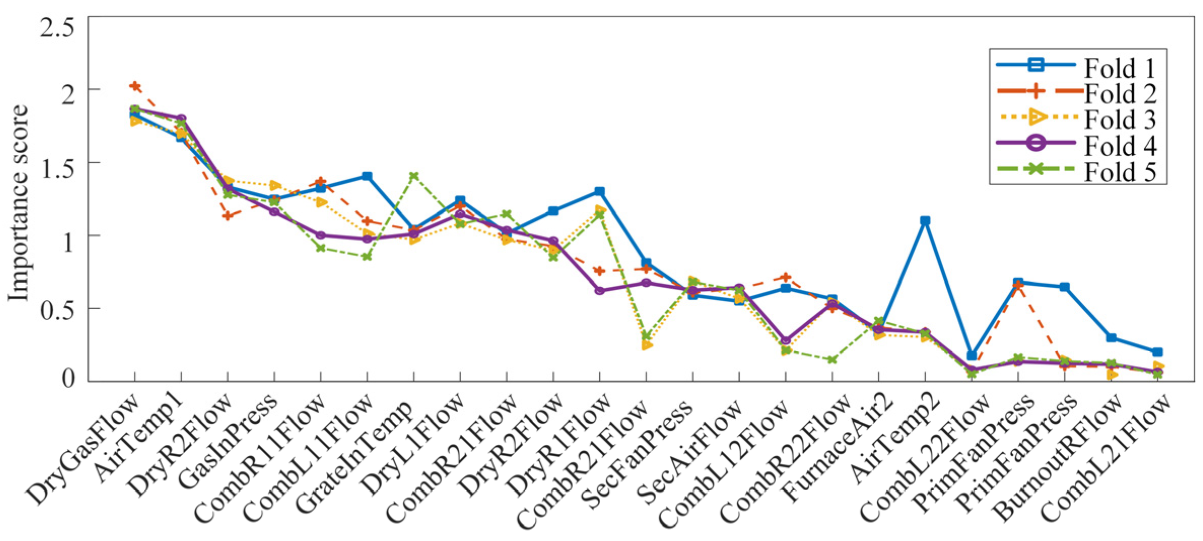
Figure 7 presents the results of the five-fold cross-validation. By combining cross-validation with the Spearman rank correlation coefficient, the relevance and robustness of the RF-based feature selection were further validated. The results indicate that the top five variables with the highest correlation were largely consistent with those identified by the RF model.

Figure 8 presents the correlation heatmap of all variables. Analysis of the heatmap indicates that the air flow variables in the drying grate series and those in the combustion grate series exhibit strong correlations.

In summary, as shown in Figure 7 and Figure 8, the results of the five-fold cross-validation are highly consistent with the RF feature importance ranking. Considering the strong correlation between the air flow at left1 and left2 grates in the drying section, seven key variables were selected as model inputs based on both statistical analysis and practical operational experience: Outlet air temperature of the primary air heater (U₁), Biogas flow rate in the drying section (U₂), Inlet biogas pressure (U₃), Air flow rate at left2 grate in the drying section (U₄), Inlet air flow in the combustion section (U₅), Feeder speed (Ω₁), and Grate speed in the combustion section (Ω₂). Among these, U₁–U₅ are high-frequency air distribution variables, capturing rapid fluctuations in airflow that affect the overall furnace temperature dynamics, while Ω₁ and Ω₂ are low-frequency material distribution variables, representing slower adjustments in fuel input and grate movement. Distinguishing high- and low-frequency variables enables the model to capture both fast and slow dynamics across the entire furnace system, consistent with the thermal characteristics and combustion mechanisms analyzed in Section 2.2.

4.2.2. Modeling and Optimization Results

Verification of Optimization Algorithm Performance

To evaluate the optimization capability of the proposed Improved Snow Ablation Optimizer (ISAO), comparative experiments were conducted using the original Snow Ablation Optimizer (SAO), Particle Swarm Optimization (PSO), and Rime Optimization Algorithm (RIME) on classical benchmark functions. In all experiments, the population size was set to 30, and the number of iterations was set to 100. Five classical benchmark functions were selected, and their specific details are listed in

Table 3. Test functions.

Function	Range
$F_1(x)={\displaystyle \sum _{i=1}^n{x}_i^2}$	[−100, 100]
$F_2\left(x\right)={\displaystyle \sum _{i=1}^n\left[100{\left(x_{i+1}-x_i^2\right)}^2+{\left(x_i+1\right)}^2\right]}$	[−30, 30]
$F_3\left(x\right)={\displaystyle \sum _{i=1}^n\left[-x_i\cdot \mathit{sin}\left(\sqrt{\left|x_i\right|}\right)\right]}$	[−500, 500]
$F_4\left(x\right)={\displaystyle \sum _{i=1}^n\left[x_i^2-10\mathit{cos}\left(2\pi x_i\right)+10\right]}$	[−5.12, 5.12]
$F_5\left(x\right)={\displaystyle \frac{\pi }{n}}\left[10{\mathit{sin}}^2\left(\pi \cdot {\displaystyle \frac{1+x_i}{4}}\right)+{\displaystyle \sum _{i=1}^n\left({\left(\frac{x_i+1}{4}\right)}^2\cdot \left(1+10{\mathit{sin}}^2\left(\pi \cdot \frac{1+x_{i+1}}{4}\right)\right)\right)+}{\left({\displaystyle \frac{x_n+1}{4}}\right)}^2\right]+{\displaystyle \sum _{i=1}^{n}U}\left(x_i,10,100,4\right)$	[−50, 50]

.

As shown by the average and best values in

Table 4. Comparison of different algorithms.

Function	Metric	RIME	PSO	SAO	ISAO
F1	Mean	8.618 × 103	3.727 × 104	5.770 × 103	4.174 × 103
	Best	1.565 × 102	1.737 × 104	3.698 × 102	5.165 × 101
F2	Mean	2.038 × 107	4.289 × 107	1.170 × 107	1.124 × 107
	Best	2.419 × 103	1.957 × 103	1.395 × 104	2.531 × 102
F3	Mean	−6.311 × 103	−2.427 × 103	−5.023 × 103	−6.697 × 103
	Best	−7.892 × 103	−2.429 × 103	−7.000 × 103	−9.453 × 103
F4	Mean	1.906 × 102	1.419 × 102	1.972 × 102	1.010 × 102
	Best	1.181 × 102	9.367 × 101	1.486 × 102	1.486 × 102
F5	Mean	2.914 × 107	1.073 × 108	3.308 × 107	1.620 × 107
	Best	2.947 × 101	1.254 × 101	2.018 × 101	2.476 × 100

, under the same number of iterations, different algorithms exhibit varying optimization performance across the benchmark functions. ISAO outperforms SAO, PSO, and RIME in both average and best results on all five functions, demonstrating superior global optimization ability. Moreover, ISAO performs particularly well on complex and nonlinear functions, showing a stronger capability to escape local optima and effectively address the optimization of key model parameters.

Orthogonal Experimental Design and Analysis of Hyperparameter Combinations

To evaluate the model’s performance under various hyperparameter combinations, an orthogonal experimental design was employed to identify effective configurations. The considered factors include Epochs, BatchSize, Hidden (number of BiLSTM hidden units), and FC Width (Fully Connected layer Width). Here, FC Width refers specifically to the width of the last fully connected layer immediately preceding the output layer, which maps the BiLSTM output to the final furnace temperature value. Each factor was set at three levels, forming a four-factor, three-level orthogonal design. To improve experimental efficiency by reducing the number of combinations, the L27 (3⁴) orthogonal table was adopted, resulting in 27 parameter combinations. Based on the comparison of experimental results across all combinations, the optimal hyperparameter configuration was selected for the final model setup.

Table 5. Orthogonal Design of Hyperparameters for Furnace Temperature Prediction.

Experiment Number	Epochs	BatchSize	Hidden	FC Width
1	100	16	32	32
2	150	16	32	32
3	200	16	32	32
…	…	…	…	…
26	150	64	128	64
27	200	64	128	128

presents the L27 orthogonal design combinations. Specifically, the factor levels were defined as follows: Epochs at 100, 150, and 200; BatchSize at 16, 32, and 64; Hidden units at 32, 64, and 128; and FC Width at 32, 64, and 128.

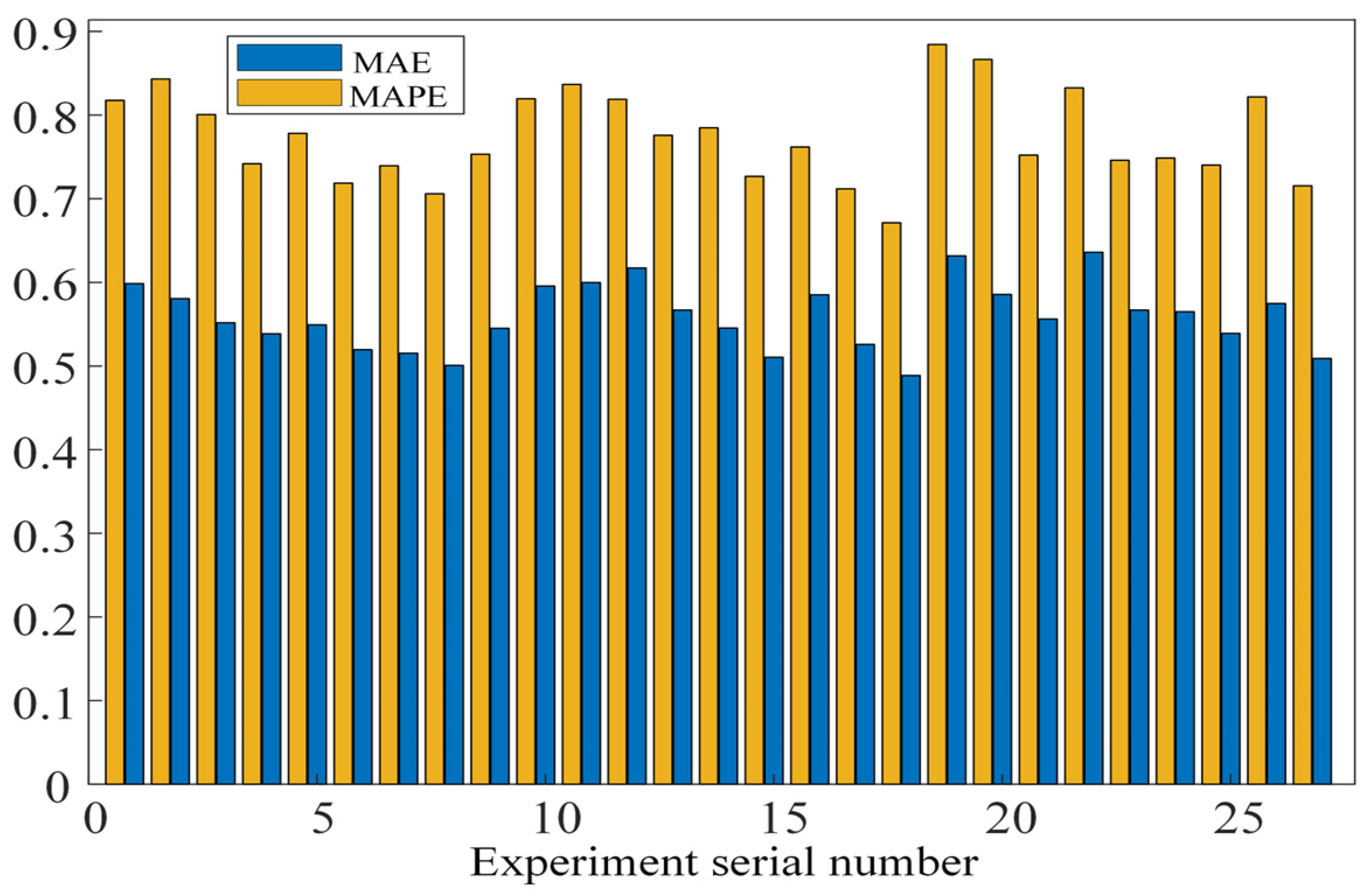
Figure 9 shows the RMSE and MAPE values corresponding to the 27 parameter combinations. It can be observed that Group 18 achieves the best performance, with the optimal configuration consisting of 200 Epochs, a batch size of 64, 64 hidden units in the BiLSTM layer, and an FC Width of 32.

This experiment demonstrates that a carefully tuned hyperparameter combination significantly improves the model’s ability to represent internal thermal processes in the MSWI furnace. The orthogonal design ensures both efficiency and objectivity in the optimization process, supporting a reliable model foundation for subsequent analysis and control.

Comparison of Temperature Models and Result Analysis

To evaluate the performance of the proposed ISAO-DBCNN-BiLSTM model, comparative experiments were conducted with BP, CNN-LSTM, CNN-BiLSTM, and dual-branch models, including DBCNN-LSTM, DBCNN-BiLSTM, and the optimization-enhanced SAO-DBCNN-BiLSTM. To ensure experimental stability and accuracy, all models were trained under the same parameter settings and with the same training dataset, and their performance was evaluated on the test set. The Adam optimizer was used for all models, with ReLU as the activation function.

Table 6. Model parameters.

Model	Parameter Name	Value
BP	Number of units	16
DBCNN	CNN1 Conv Layer 1 Channels	16
	CNN1 Conv Layer 2 Channels	32
	CNN2 Channels	32
	Convolution Kernel Size	[3 × 1]
LSTM	Hidden	64
BiLSTM	Hidden	64
DBCNN-BiLSTM	Epochs	200
	$\delta$	0.5
	$\eta$	0.001

presents the parameter settings for each model.

ISAO was employed to optimize two key hyperparameters of the model. In practical operation, the algorithm requires relatively few iterations to reach convergence; therefore, the number of iterations was set to 10, and the population size was set to 10.

For efficiency, the optimization phase used a subset of the training set consisting of approximately 70 percent of the samples. A small number of training epochs was used to quickly evaluate candidate solutions. Parallel training was applied to evaluate multiple candidates at the same time. All experiments were conducted on a workstation with an AMD Ryzen 9 7945HX CPU at 2.50 GHz, 16 GB RAM, and an NVIDIA GeForce RTX 4060 Laptop GPU running a 64-bit operating system. Under these conditions, the total optimization time ranged from approximately 30 to 40 min. This time includes training and validation of all candidate solutions. Using the optimized key parameters, a full run of the DBCNN-BiLSTM model, including training on the entire training set and evaluation on the validation and test sets, required roughly 4 to 5 min per run. The use of ISAO allows the model to achieve better prediction accuracy compared to manual tuning or conventional search methods while keeping the computational cost acceptable. Optimization can be performed offline and updated periodically, which makes it practical for engineering applications.

Table 7. Optimized Key Hyperparameters of the Model.

Hyperparameter	Optimized Value
$\delta$	0.1016
$\eta$	0.005131

presents the results of the optimized key parameters obtained by ISAO.

Table 8. Comparison of seven models.

Model	RMSE	MAE	MAPE	R2
BP	3.6202	2.4049	0.2527	0.9284
CNN-LSTM	1.5259	1.1523	0.1282	0.9873
CNN-BiLSTM	1.5057	1.2146	0.1398	0.9876
DBCNN-LSTM	1.4452	1.1081	0.1256	0.9882
DBCNN-BiLSTM	1.4252	1.0789	0.1139	0.9889
SAO-DBCNN-BiLSTM	1.2860	0.9878	0.1037	0.9916
ISAO-DBCNN-BiLSTM	1.1835	0.8819	0.0927	0.9923

presents the error comparison of different models in furnace temperature modeling. The table includes the RMSE, MAE, MAPE, and R² for each model. Figure 10 and Figure 11 show the fitting comparison results of the models listed in Table 6. As can be seen from Table 8 and Figure 10 and Figure 11, the BP neural network exhibits the largest fitting errors, indicating that traditional neural networks are inadequate for modeling furnace temperature under complex and variable operating conditions.

In contrast, deep learning models demonstrate clear advantages in modeling furnace temperature under variable operating conditions, enhancing the capability for complex feature extraction and temporal dependency modeling. A comparison of the four models—CNN-LSTM, CNN-BiLSTM, DBCNN-LSTM, and DBCNN-BiLSTM—reveals that within the CNN framework, the CNN-BiLSTM model achieves slight improvements in RMSE and R² compared to CNN-LSTM, indicating stronger global fitting ability and better modeling of contextual dependencies. However, its MAE and MAPE increase to 1.2146 and 0.1398, respectively, reflecting slightly inferior performance in controlling local errors compared to CNN-LSTM.

As discussed above, although BiLSTM has certain advantages in capturing bidirectional temporal features, the model’s fitting stability still has room for improvement when handling small-sample intervals or high-frequency fluctuations.

With the introduction of the dual-branch convolutional structure, the accuracy of both models is significantly enhanced. The RMSE of DBCNN-LSTM is 1.4452, representing a 5.29% reduction compared to CNN-LSTM. For DBCNN-BiLSTM, the RMSE further decreases to 1.4252; compared with DBCNN-LSTM, the MAE drops from 1.1081 to 1.0789, and the MAPE decreases from 0.1256 to 0.1139. R² is further improved, indicating that the dual-branch structure enhances the model’s fitting capability under complex operating conditions.

On this basis, to further enhance model performance, an optimization algorithm was introduced to tune the key parameters of the model. After incorporating SAO, the RMSE decreased by approximately 18.10% compared to the unoptimized DBCNN-BiLSTM model. Replacing SAO with the improved ISAO further reduced the RMSE to 1.1835, improving both the fitting accuracy and stability of the model.

Figure 12 presents the autocorrelation function of the normalized deviations between the model-predicted furnace temperatures and the measured values. Most of the autocorrelation coefficients of the deviation sequence fall within the 95% confidence interval, accounting for 96.2% of the data. Therefore, the residual sequence can be considered as white noise, demonstrating that the proposed temperature model achieves high modeling accuracy and stability.

The above experimental results indicate that the ISAO-DBCNN-BiLSTM model achieves high accuracy and stability in modeling furnace temperature under variable operating conditions. At the same time, it provides practical guidance for MSWI operational strategies. By identifying high-frequency air distribution variables and low-frequency feeding variables, operators can focus on key control points, such as primary air regulation and feeder speed adjustment, to improve furnace responsiveness and efficiency. The connection between model outputs and operational parameters bridges the gap between data-driven modeling and actual process control. In addition, through key parameter optimization, the model maintains robustness under different operating conditions. This provides a basis for dynamic adjustment of operational strategies and supports the development of future multi-objective control and optimization frameworks.

5. Conclusions

To address the challenges of furnace temperature measurement in MSWI under variable operating conditions—such as large data fluctuations and difficulty in accurate modeling—this study proposes an MSWI furnace temperature model based on ISAO-integrated DBCNN-BiLSTM. The model employs a dual-branch CNN structure to separately process high-frequency air distribution variables and low-frequency material distribution variables, while BiLSTM captures the temporal dependencies in the sequential data. To further enhance model adaptability and generalization, the ISAO algorithm is introduced to optimize the key hyperparameters, achieving a coordinated optimization of both model structure and parameter configuration. This approach effectively strengthens the model’s capability for dynamic furnace temperature modeling. Experimental results demonstrate that the proposed ISAO-DBCNN-BiLSTM model outperforms other deep learning comparison models across multiple evaluation metrics.

Despite achieving promising results in the nonlinear modeling of furnace temperature, this study still has several limitations and areas for improvement. First, the model is highly sensitive to the quality of input data. In real operating conditions, spatial disturbances may degrade data quality, which could affect the stability and accuracy of temperature modeling. Second, although multiple improvement strategies were introduced to enhance the optimization precision of ISAO, the convergence speed of the algorithm has decreased. Although the current total computational cost remains acceptable, there is still room for further efficiency improvement. Third, the dataset used in this study was collected from a single MSWI plant in China, which may limit the generalizability of the results. In particular, plant-specific factors such as variability in waste calorific value, moisture content, and plant-specific operational strategies could lead to different furnace temperature dynamics, thereby constraining the external applicability of the model. Finally, the current model focuses on a single output—furnace temperature—and does not fully account for the interactions between temperature and other operational objectives, which represents a limitation of the present approach.

Future research will focus on further enhancing the model’s robustness and generalization capability to improve prediction accuracy under complex operating conditions. To address the issue of optimization efficiency, multi-strategy co-evolution mechanisms or parallel optimization frameworks will be explored to maintain high precision in parameter optimization while accelerating convergence. In addition, expanding validation across multiple MSWI plants with different waste compositions and operating conditions will be pursued, potentially incorporating transfer learning or domain adaptation to improve applicability. Moreover, a multi-objective modeling and optimization framework tailored for MSWI systems will be developed, integrating key targets such as furnace temperature, pollutant emissions, and thermal efficiency into a unified optimization process, thereby promoting the intelligent and green operation of municipal solid waste incineration.

References

1. Khan, S.; Anjum, R.; Raza, S.T.; Ahmed Bazai, N.; Ihtisham, M. Technologies for Municipal Solid Waste Management: Current Status, Challenges, and Future Perspectives. Chemosphere 2022, 288, 132403. [Google Scholar] [CrossRef]
2. Sun, J.; Meng, X.; Qiao, J. Data-Driven Optimal Control for Municipal Solid Waste Incineration Process. IEEE Trans. Ind. Inform. 2023, 19, 11444–11454. [Google Scholar] [CrossRef]
3. Beylot, A.; Hochar, A.; Michel, P.; Descat, M.; Ménard, Y.; Villeneuve, J. Municipal Solid Waste Incineration in France: An Overview of Air Pollution Control Techniques, Emissions, and Energy Efficiency. J. Ind. Ecol. 2018, 22, 1016–1026. [Google Scholar] [CrossRef]
4. Yang, Q.; Zhu, Y.; Liu, X.; Fu, L.; Guo, Q. Bayesian-Based NIMBY Crisis Transformation Path Discovery for Municipal Solid Waste Incineration in China. Sustainability 2019, 11, 2364. [Google Scholar] [CrossRef]
5. Chen, S.; Liu, J.; Lin, Z. Atmosphere-Dependent Pyrolytic Transformability of Glass Fiber/Epoxy Resin Composites in Waste Wind Turbine Blades. Chem. Eng. J. 2025, 505, 159675. [Google Scholar] [CrossRef]
6. Lin, S.; Li, L.; Liu, J. CO2-Induced Co-Pyrolysis of Pennisetum Hydridum and Waste Tires: Multi-Objective Optimization of Its Synergies and Pyrolytic Oil, Char and Gas Outputs. Energy 2025, 317, 134670. [Google Scholar] [CrossRef]
7. Tian, H.; Tang, J.; Wang, T. Furnace Temperature Model Predictive Control Based on Particle Swarm Rolling Optimization for Municipal Solid Waste Incineration. Sustainability 2024, 16, 7670. [Google Scholar] [CrossRef]
8. Sarakikya, H.; Mashingo, P.; Kilonzo, F. Design and Computational Fluid Dynamics Modeling for a Municipal Solid Waste Incineration Process. Open J. Fluid Dyn. 2021, 11, 177–191. [Google Scholar] [CrossRef]
9. Magnanelli, E.; Tranås, O.L.; Carlsson, P.; Mosby, J.; Becidan, M. Dynamic Modeling of Municipal Solid Waste Incineration. Energy 2020, 209, 118426. [Google Scholar] [CrossRef]
10. Yan, A.; Guo, J.; Wang, D. Heterogeneous Feature Ensemble Modeling with Stochastic Configuration Networks for Predicting Furnace Temperature of a Municipal Solid Waste Incineration Process. Neural Comput. Appl. 2022, 34, 15807–15819. [Google Scholar] [CrossRef]
11. Wen, C.; Lin, X.; Ying, Y.; Ma, Y.; Yu, H.; Li, X.; Yan, J. Dioxin Emission Prediction from a Full-Scale Municipal Solid Waste Incinerator: Deep Learning Model in Time-Series Input. Waste Manag. 2023, 170, 93–102. [Google Scholar] [CrossRef]
12. Huang, W.; Ding, H.; Qiao, J. Large-Scale and Knowledge-Based Dynamic Multiobjective Optimization for MSWI Process Using Adaptive Competitive Swarm Optimization. IEEE Trans. Syst. Man Cybern. Syst. 2024, 54, 379–390. [Google Scholar] [CrossRef]
13. Qiu, B.; Yuan, Q.; Niu, Y.; Mo, H.; Sun, C.; Feng, J. Prediction of NOx Emissions from Co-Disposal of Municipal Solid Waste and Sludge Using a GA-LSTM Neural Network. Environ. Technol. 2025, 46, 4475–4492. [Google Scholar] [CrossRef]
14. Li, Z.; Yu, Z.; Chen, D.; Li, L.; Lu, Z.; Yao, S. Soft Sensing of NOx Emission from Waste Incineration Process Based on Data De-Noising and Bidirectional Long Short-Term Memory Neural Networks. Waste Manag. Res 2025, 43, 602–615. [Google Scholar] [CrossRef]
15. Zhao, Z.; Zhou, Z.; Lu, Y.; Li, Z.; Wei, Q.; Xu, H. Predictions of the Key Operating Parameters in Waste Incineration Using Big Data and a Multiverse Optimizer Deep Learning Model. Sustainability 2023, 15, 14530. [Google Scholar] [CrossRef]
16. Xia, H.; Tang, J.; Yu, W.; Qiao, J. Hybrid Simulator-Based Mechanism and Data-Driven for Multidemand Dioxin Emissions Intelligent Prediction in the MSWI Process. IEEE Trans. Ind. Electron. 2024, 71, 13221–13231. [Google Scholar] [CrossRef]
17. Chen, G.; Yin, D.; Chen, F. Collaborative Multi-Objective Optimization of Combustion and Emissions in Circulating Fluidized Bed Boilers Using the Bidirectional Temporal Convolutional Network and Hybrid Dung Beetle Optimizer. Sustainability 2025, 17, 5225. [Google Scholar] [CrossRef]
18. Ding, H.; Tang, J.; Qiao, J. Dynamic Modeling of Multi-Input and Multi-Output Controlled Object for Municipal Solid Waste Incineration Process. Appl. Energy 2023, 339, 120982. [Google Scholar] [CrossRef]
19. Ji, Z.; Tao, W.; Ren, J. Boiler Furnace Temperature and Oxygen Content Prediction Based on Hybrid CNN, biLSTM, and SE-Net Models. Appl. Intell. 2024, 54, 8241–8261. [Google Scholar] [CrossRef]
20. Xu, S.; Yao, Y.; Yong, N.; Xia, D.; Ge, D.; Yu, J. Intelligent Multi-Severity Nuclear Accident Identification under Transferable Operation Conditions. Ann. Nucl. Energy 2024, 201, 110416. [Google Scholar] [CrossRef]
21. Wu, Y.; Xiang, C.; Qian, H.; Zhou, P. Optimization of Bi-LSTM Photovoltaic Power Prediction Based on Improved Snow Ablation Optimization Algorithm. Energies 2024, 17, 4434. [Google Scholar] [CrossRef]
22. Wang, Z.; Tang, Y.; Zhang, Z. Dual-Branch Deep Learning Architecture for Enhanced Hourly Global Horizontal Irradiance Forecasting. Expert Syst. Appl. 2024, 252, 124115. [Google Scholar] [CrossRef]
23. Shi, X.; Huang, G.; Hao, X.; Yang, Y.; Li, Z. Sliding Window and Dual-Channel CNN (SWDC-CNN): A Novel Method for Synchronous Prediction of Coal and Electricity Consumption in Cement Calcination Process. Appl. Soft Comput. 2022, 129, 109520. [Google Scholar] [CrossRef]
24. Deng, L. Snow Ablation Optimizer: A Novel Metaheuristic Technique for Numerical Optimization and Engineering Design. Expert Syst. Appl. 2023, 225, 120069. [Google Scholar] [CrossRef]
25. Ismaeel, A.A.K.; Houssein, E.H.; Khafaga, D.S.; Aldakhee, E.A.; AbdElrazek, A.S.; Said, M. Performance of Snow Ablation Optimization for Solving Optimum Allocation of Generator Units. IEEE Access 2024, 12, 17690–17707. [Google Scholar] [CrossRef]
26. Cui, L.; Hu, G.; Zhu, Y. Multi-Strategy Improved Snow Ablation Optimizer: A Case Study of Optimization of Kernel Extreme Learning Machine for Flood Prediction. Artif. Intell. Rev. 2025, 58, 181. [Google Scholar] [CrossRef]
Figure 1. MSWI process flow.
Sustainability 17 08457 g001
Figure 2. Input–Output Relationship Diagram of the Furnace Temperature Model in the Incineration Process.
Sustainability 17 08457 g002
Figure 3. Comparison of Adjustment Frequencies of Seven Variables Related to Furnace Temperature.
Sustainability 17 08457 g003
Figure 4. Furnace temperature prediction strategy based on DBCNN-BiLSTM optimized by ISAO.
Sustainability 17 08457 g004
Figure 5. Flowchart of the ISAO-DBCNN-BiLSTM Temperature Prediction Model.
Sustainability 17 08457 g005
Figure 6. RF importance ranking.
Sustainability 17 08457 g006
Figure 7. 5-fold cross-validation.
Sustainability 17 08457 g007
Figure 8. Heatmap.
Sustainability 17 08457 g008
Figure 9. Comparison of MAE and MAPE under Different Hyperparameter Combinations.
Sustainability 17 08457 g009
Figure 10. Comparison of Modeling Results Across Different Models.
Sustainability 17 08457 g010
Figure 11. Comparison of Modeling Results of Optimized Models.
Sustainability 17 08457 g011
Figure 12. Autocorrelation function of furnace temperature prediction model deviation.
Sustainability 17 08457 g012