Article

Dynamic Optimization of Highway Emergency Lane Activation Using Kriging Surrogate Modeling and NSGA-II

by
Yi Fei
,
Yanan Wang
and
Qiuyan Zhang
*
College of Applied Mathematics, Chengdu University of Information Technology, Chengdu 610225, China
*
Author to whom correspondence should be addressed.
Sustainability 2025, 17(18), 8327; https://doi.org/10.3390/su17188327
Submission received: 24 August 2025 / Revised: 12 September 2025 / Accepted: 15 September 2025 / Published: 17 September 2025

Abstract

Highway congestion is a persistent issue, and dynamically activating emergency lanes offers a promising mitigation strategy. However, traditional fixed-time or single-threshold methods often fail to balance traffic efficiency and safety. This paper introduces a dynamic optimization framework that integrates a Kriging surrogate model with the Non-dominated Sorting Genetic Algorithm II (NSGA-II) to identify optimal activation strategies. By simultaneously minimizing total travel time (efficiency) and the duration vehicles spend in unsafe proximity (safety), our method generates a set of Pareto-optimal solutions. We calibrated and validated the model using real-world highway data. The results are compelling: the optimized compromise strategy reduced total travel time by 20.5% compared to having no activation, while keeping safety risks within an acceptable range. The use of a Kriging surrogate model sped up the optimization process by approximately 20 times compared to direct simulation, achieving a prediction accuracy of 97.8%. The optimal strategies characteristically involve opening the emergency lane at the downstream bottleneck during peak congestion and closing it promptly as traffic eases. This research provides a robust, efficient, and practical decision-support tool for intelligent traffic management, offering a clear pathway to safer and less congested highways.

1. Introduction

Highway emergency lanes are typically reserved for incident management and special vehicle access, but they are not open to regular traffic. However, in saturated high-flow sections, temporary opening of emergency lanes can increase the effective number of lanes in a short time, alleviating bottleneck congestion and improving throughput. Various activation strategies have been implemented worldwide, from static predetermined schedules to emerging dynamic methods, as will be further explored in Section 2.1. However, these control methods mostly involve static, predetermined time periods, suitable only for highly predictable congestion patterns. While static methods are straightforward, they fail to address the randomness and suddenness of highway congestion, potentially leading to ineffective activation or safety risks during non-congested times. Therefore, it is necessary to dynamically decide on the activation and deactivation of emergency lanes based on real-time traffic conditions, enhancing the specificity and safety of activation decisions.
Recent research on dynamic emergency lane activation has gradually developed in China. Threshold-based methods have been proposed and implemented, as exemplified by Yang et al.’s work [1], which will be discussed in detail in Section 2.1. While this type of threshold-based model is simple and practical, it faces a fundamental limitation in balancing traffic efficiency and safety simultaneously: a threshold that is too high may delay activation timing, while one that is too low might open emergency lanes before severe congestion occurs, increasing accident risk. This limitation highlights the need for more advanced optimization approaches that consider multiple objectives. Therefore, there is an urgent need for an optimization method guided by efficiency-safety dual objectives to comprehensively determine emergency lane activation strategies based on traffic operating conditions.
To this end, we develop a multi-objective optimization framework for dynamic emergency lane activation, integrating Pareto optimality analysis with real-time traffic state estimation. On one hand, traffic efficiency and safety serve as optimization objectives: the former can be measured through vehicle delay or travel time, while the latter can be assessed through conflict probability or duration of dangerous states. Due to the scarcity of actual accident data, safety margin indicators such as Time-to-Collision (TTC) are commonly used as alternative evaluations for traffic safety [2]. In particular, Minderhoud and Bovy proposed indicators such as Time Exposed Time-to-collision (TET) and Time Integrated Time-to-collision (TIT), which statistically record the duration when a vehicle’s TTC is below a threshold, to quantify the risk of prolonged dangerous following distances [3]. These indicators can be extracted from simulation trajectories to characterize the safety impact of emergency lane activation. On the other hand, regarding optimization methods, since multiple evaluation indicators need to be considered simultaneously and traffic flow simulation is highly complex, we use genetic algorithms for multi-objective search and introduce Kriging surrogate models (also known as Gaussian process regression) to approximate simulation models and accelerate the optimization process [4,5]. Genetic algorithms efficiently search for global optimal solutions through population evolution mechanisms and have been widely used in traffic control optimization; improved multi-objective genetic algorithms such as Non-dominated Sorting Genetic Algorithm II (NSGA-II) can obtain a set of Pareto-optimal solutions for decision-makers to choose from [6]. The Kriging surrogate model, as a probabilistic global proxy, can learn the nonlinear mapping relationship between traffic simulation inputs and outputs through a small number of samples [7]. In engineering optimization, the Kriging surrogate model is often combined with evolutionary algorithms to reduce the number of evaluation function calls [8]. Introducing it into this problem can significantly reduce the number of simulation evaluations while maintaining accuracy, thereby improving optimization efficiency.
In this paper, we establish an optimization model for highway emergency lane dynamic activation strategies around the dual objectives of “efficiency-safety” and propose corresponding solution algorithms. The innovations include: (1) We incorporate traffic efficiency and safety risk into a unified framework and seek optimization through multi-objective genetic algorithms, avoiding the problem of single threshold methods that struggle to balance dual objectives; (2) We use Kriging surrogate models to reduce complex traffic simulation computational overhead, improve optimization solution speed, and introduce cross-validation and prediction interval analysis to enhance surrogate model reliability; (3) We calibrate the model based on real traffic data, conduct in-depth analysis of data characteristics to ensure that simulation and optimization results have practical reference value.
This paper aims to address the aforementioned gaps by developing a comprehensive bi-objective optimization framework. Specifically, we seek to answer the following research questions (Research Questions; hereafter, “RQ”):
RQ1: How can traffic efficiency (minimizing total travel time) and safety (minimizing risk exposure) be simultaneously optimized for the dynamic activation of highway emergency lanes?
RQ2: Can a surrogate model-assisted evolutionary algorithm provide a computationally efficient method for finding a set of Pareto-optimal activation strategies, making it viable for practical application?
RQ3: How do optimized policies translate into simple, operable rules for control centers?
RQ4: How sensitive are decisions to the TTC threshold and demand uncertainty?
To answer these, we test the following hypotheses:
H1 (Trade-off):
Dynamic activation exhibits a measurable efficiency-safety trade-off (Pareto frontier).
H2 (Surrogate fidelity):
A Kriging surrogate fitted on ≤100 samples attains R 2 0.93 and preserves the Pareto set.
H3 (Policy distillation):
A simplified rule derived from the Pareto set retains ≥95% efficiency and ≥97% safety performance of the optimized policy.
H4 (Robustness):
Qualitative policy patterns remain stable for τ [ 2 , 4 ] s and ±10% demand changes.
By addressing these questions and hypotheses, this study provides not only a methodological advancement but also a practical, data-driven tool for highway traffic management.
We organize the remainder of this paper as follows: In Section 2, we review related research progress; in Section 3, we introduce our proposed model construction and algorithm design, including traffic flow simulation techniques, Kriging surrogate model implementation, and genetic algorithm procedures; in Section 4, we describe the experimental data, parameter calibration processes, and simulation platform development for implementing optimization solutions; in Section 5, we present comprehensive optimization results and analysis, including convergence characteristics, optimization strategy features, and sensitivity analysis; in Section 6, we discuss the application prospects, practical challenges, and limitations of our proposed method; and finally, we summarize the main contributions of this paper and outline directions for future research.

2. Literature Review

2.1. Emergency Lane Activation Strategies and Threshold-Based Research

Foreign research and practices regarding Hard Shoulder Running (HSR) on highways began earlier. European and American countries started experimenting with allowing vehicles to use emergency lanes during traffic peaks in the early 21st century to increase capacity. For example, the United Kingdom borrowed emergency lanes as bus lanes [9], while Germany dynamically opened hard shoulders to all vehicles in certain congested sections [10]. Some scholars conducted comprehensive evaluations of hard shoulder dynamic management systems in the United States and six European countries, finding that HSR can increase capacity by 7–25% and reduce traffic delays by 25% [11]. These early strategies mostly adopted fixed opening periods or specific vehicle types, constituting static control methods.
In recent years, dynamic activation of emergency lanes has received attention, with researchers beginning to explore activation decision models based on real-time traffic conditions [12,13]. The intelligent traffic management system developed by Highways England has implemented automatic shoulder management based on flow and speed thresholds [14]. Yang et al. [1] analyzed historical data from the Wuxi section of the Shanghai-Nanjing Expressway, calculating the probability distribution of congestion under different speed and flow combinations, determining that when average speed falls below 60 km/h, the section is already in a congested state, while 60–80 km/h represents a potentially congested interval; they also found that when single-lane flow reaches 1600 veh/h, the probability of congestion occurring within 15 min exceeds 50% [1]. Accordingly, they proposed criteria for dynamically opening emergency lanes: speed below 60 km/h and flow exceeding 1600 veh/(h·ln). In practical applications, in 2019, the Wuxi section of the Shanghai-Nanjing Expressway took the lead in implementing dynamic emergency lane management, with control personnel deciding whether to open emergency lanes by section along the 42 km stretch based on real-time flow and congestion conditions. This method essentially uses empirical thresholds as opening and closing rules, with the advantages of being intuitive and easy to implement. However, simple thresholds struggle to account for complex multi-factor influences: besides flow and speed, consideration should also be given to congestion duration, queue length, and safety conditions [15]. Particularly in terms of safety, relying solely on speed thresholds makes it difficult to assess changes in accident risk after opening emergency lanes. Therefore, scholars have begun to consider integrating multiple indicators for decision-making, proposing the establishment of congestion indices or service level evaluations that synthesize factors such as speed and density into grades, opening emergency lanes when severe congestion grades are reached.
Recent studies from 2022–2024 have advanced HSR with multi-objective optimization. For instance, Arora et al. (2023) integrated variable speed limits with dynamic HSR to optimize operational impacts, focusing on safety through crash prediction models [12]. Yao et al. (2024) proposed a Hidden Markov Model-based strategy for HSR in hybrid networks, emphasizing efficiency under uncertainty [13]. Abdel-Aty et al. (2024) developed a transformer-based real-time crash prediction for combined HSR and variable speed limits [16]. Unlike these recent HSR studies, which often prioritize single objectives or lack scalable multi-objective exploration, we consider efficiency and safety simultaneously from a multi-objective optimization perspective, seeking a Pareto-optimal strategy set by establishing a precise optimization model, transcending the limitations of single threshold triggering.

2.2. Traffic Flow Modeling and Simulation Methods

Reliable traffic flow models are needed to research emergency lane activation strategies. Macroscopic models can characterize traffic flow evolution with relatively low computational cost. We select the CTM for macroscopic traffic simulation [17]. CTM is a discrete dynamic model based on flow conservation and simplified fundamental diagrams, proposed by Daganzo and proven to be a Godunov discretization format of the continuous traffic flow model (LWR model) [18,19]. Its basic idea is to divide roads into several cells, with each cell’s length taken as the distance a vehicle travels in one time step under free-flow conditions [20]. Each cell has a corresponding flow-density function (fundamental diagram), typically adopting a triangular fundamental diagram parameterized by free-flow speed v f , congestion wave speed w, and maximum flow q max (capacity). CTM calculates the vehicle transfer flow between adjacent cells at each discrete time step based on the supply capacity of adjacent cells and demand flow rate, then updates each cell’s vehicle inventory (density) [21]. This process can simulate the transformation from free flow to congested flow and the propagation and overflow of queues in space.
Sumalee et al. [22] developed a stochastic CTM model, considering the randomness of traffic flow, providing a foundation for traffic control under uncertain conditions. Li et al. [23] used CTM to evaluate the effectiveness of variable speed limit strategies, finding that reasonable speed control can effectively reduce congestion time and range. Since emergency lane opening increases cross-sectional capacity, we model this effect by adjusting CTM fundamental diagram parameters: when an emergency lane is activated in a certain section, the q max and jam density k j of that section are scaled up according to the ratio of main lanes plus emergency lane to main lanes (e.g., from 2 lanes to 3 lanes, q max is multiplied by 1.5) to simulate the impact of lane addition on flow. It should be noted that macroscopic models have difficulty directly producing detailed safety indicators, so we combine microscopic simulation to extract TTC indicators, using macroscopic models for efficiency assessment and microscopic models for safety assessment, complementing each other. Overall, the CTM model has the advantages of being simple, efficient, and capable of reflecting basic congestion dynamics, and we use it in this study to quickly predict the performance of different emergency lane activation schemes in terms of traffic efficiency.

2.3. Traffic Safety Evaluation and TTC Indicator Applications

Road safety is usually evaluated through accident rate statistics, but for pre-assessment of new strategies, accident data is often insufficient, necessitating conflict simulation methods. TTC is a commonly used conflict criterion, representing the time needed for two vehicles to collide if they maintain their current speed and trajectory. Hayward [24] first proposed the concept of TTC as a traffic conflict evaluation indicator, suggesting that TTC < 1.5 s could be considered a dangerous state. When TTC is below a certain threshold (such as 3 s), it indicates that two vehicles are in a state of dangerous proximity. Indicators derived from TTC have been developed to assess safety risks over a period of time, such as TET and TIT [3,16]. TET measures the total duration when a vehicle’s TTC is below the threshold, while TIT accumulates (integrates) the remaining TTC in situations below the threshold to obtain a comprehensive risk value. Recent trajectory-based studies, such as Li et al. [25], further validate TTC-type indicators for quantifying lane-changing risks under varying environmental conditions (e.g., weather impacts), aligning with our extraction of TET from hybrid macro-micro simulations. These indicators can be calculated in real-time in microscopic traffic simulations [26].
In emergency lane activation scenarios, due to the availability of an additional lane, average vehicle headways may shorten, lane-changing frequency may increase, and potential conflict situations may also increase [12,15]. Therefore, using TET as one of the safety objectives can constrain the algorithm from pursuing efficiency at the expense of neglecting safety. Moreover, recent trajectory-based studies show that microscopic behaviors exhibit significant differences across scenarios (lane counts, lane-changing directions, vehicle classes, and speed limits), and such differences should be established via formal statistical significance tests rather than descriptive summaries alone [27]. Existing research has shown that using TTC-type indicators for safety assessment in intelligent driving or traffic control is feasible [28].
We will record the TTC changes of all following vehicles during simulation, cumulatively calculating total TET as an indicator to measure the overall safety risk of traffic flow after emergency lane activation. To ensure that observed efficiency–safety differences are not artifacts of sampling variability, we follow [27] and, in Section 5, first check homoscedasticity and then apply appropriate parametric or non-parametric tests at the 95% confidence level when comparing extreme and representative strategies. Thus, safety evaluation is consistently incorporated into and statistically validated within the optimization framework.

2.4. Multi-Objective Optimization Algorithms and Surrogate Model Applications

Genetic Algorithms (GA) are widely used in combinatorial optimization problems such as traffic signal control and path optimization due to their robust global search performance. NSGA-II is a well-established multi-objective genetic algorithm proposed by Deb et al. [6], employing fast non-dominated sorting and crowding distance comparison strategies to approach the Pareto front while maintaining solution set diversity. Zhou et al. [29] demonstrated through case studies that applying genetic algorithms can effectively solve multi-objective optimization problems of intersection signal timing, achieving good results in reducing delay, fuel consumption, and emissions. While other heuristic algorithms, such as simulated annealing or particle swarm optimization, have also been applied to traffic optimization problems, GA, and specifically NSGA-II, is particularly well-suited for this study. Its strengths lie in efficiently exploring complex, non-convex, and multi-modal solution spaces and its inherent ability to generate a diverse set of Pareto-optimal solutions, which is essential for trade-off analysis in multi-objective problems like balancing traffic efficiency and safety.
For simulation-driven optimization problems, GA requires running a simulation each time an individual is evaluated, resulting in a high computational cost. For this reason, surrogate models (metamodels) can be introduced to replace some simulation evaluations [30]. Osorio and Bierlaire [31] used surrogate models to replace microscopic simulation in traffic network optimization, significantly reducing computation time while maintaining solution quality. The Kriging surrogate model is a commonly used high-precision metamodel, constructed by Gaussian process regression, providing prediction mean and variance when fitting training sample data [32]. Compared to simple models such as polynomial response surfaces, Kriging can more accurately reflect complex response surface relationships and consider the spatial correlation of various input variables through correlation functions.
Forrester et al. [33] systematically introduced surrogate model-assisted optimization methods, particularly emphasizing the application value of Kriging models in complex engineering optimization. In engineering optimization, Kriging is often combined with the Expected Improvement (EI) criterion for global optimization, namely the famous EGO algorithm [34]. Liu et al. [35] developed multi-fidelity Kriging models, combining high-precision and low-precision simulation data to maintain prediction accuracy while reducing the number of high-precision simulations. We do not adopt EI adaptive sampling but instead use the “surrogate model + genetic algorithm” framework: first building models offline, then using genetic algorithms to quickly optimize on the surrogate model [36]. In the transportation field, applications of surrogate models have begun to appear, such as Li et al. [37] developing a dedicated global optimization algorithm for car-following model calibration problems. However, for problems requiring simulation verification, like emergency lane activation, Kriging surrogate models are more applicable with their good generalization ability under small samples and provision of prediction uncertainty estimates. By reducing the number of simulations through surrogate models, optimization solution efficiency can be greatly improved, making it possible to consider complex safety and efficiency objectives simultaneously.

3. Models and Methods

3.1. Problem Description and Model Construction

3.1.1. Scenario Assumptions

Consider a closed saturated highway section, approximately 5 km in total length, with 2 main lanes and 1 emergency lane (normally closed). This 5 km extent was specifically chosen as it matches the spacing of four existing CCTV gantries on our study corridor and encompasses the observed maximum queue spillback of 2–3 km during peak hours, ensuring the control horizon fully contains the bottleneck dynamics without boundary effects. The “2 main + 1 shoulder” configuration represents a standard highway design widely adopted in freeway systems, making our findings broadly applicable. Four video observation points are deployed along the route, located at the starting point (observation point 1), 1 km downstream (observation point 2), 2 km downstream (observation point 3), and the endpoint (observation point 4). This infrastructure alignment ensures complete observability while matching typical variable message sign spacing, enabling practical implementation of segment-specific activation strategies.
Based on the actual road conditions, we divide the section into 3 decision segments, each corresponding to a decision unit for whether to activate the emergency lane. To correspond with observation point locations, we take the section between observation points 1–2 as the first segment, between points 2–3 as the second segment, and between points 3–4 as the third segment (approximately 3 km long). Temporally, the decision horizon is discretized into several equal-length decision cycles (such as 5 min per cycle). Thus, an emergency lane activation strategy can be represented as a two-dimensional spatiotemporal matrix X = [ x i , t ] , where x i , t { 0 , 1 } indicates whether the emergency lane is activated in the i-th spatial segment during the t-th time cycle.

3.1.2. Optimization Objectives

Strategy optimization is guided by dual objectives of driving efficiency and safety risk, establishing a bi-objective function:
  • Driving Efficiency Objective: Measured using TTT, equivalent to the sum of time spent by all vehicles traveling through the section. A smaller TTT indicates higher overall traffic efficiency. If N vehicles pass through the study section during the simulation observation period, and the j-th vehicle spends time T j in the section (calculated from the difference between entry and exit times), TTT = j = 1 N T j . Since total travel time positively correlates with road delay, equivalent indicators such as total or average delay can also be used. This model is designed to minimize TTT as one objective, i.e.,
    min F 1 ( X ) = TTT ( X )
  • Safety Risk Objective: Measured using the TET indicator, defined as: the cumulative sum of time periods when all vehicles’ TTC is below a safety threshold τ during the simulation period [3]. Intuitively, a larger TET indicates longer cumulative time that vehicles are in potential collision danger, resulting in poorer traffic safety. During calculation, the TTC time series must be extracted from the vehicle following process. When the following vehicle’s TTC is less than the threshold (e.g., τ = 3 s), its duration is recorded and added to the TET. The total TET is obtained by repeated accumulation for multiple vehicles and multiple time points. We aim to minimize total exposure time, i.e.,
    min F 2 ( X ) = TET ( X )
    It should be noted that the choice of threshold τ will affect the magnitude of TET values. Typically, for passenger car following, TTC = 3 s is used as one criterion for danger assessment, with TTC falling below 1 s considered extremely high risk [28]. We refer to common standards, taking τ = 3 s, with the sensitivity analysis section discussing the impact of threshold changes.
The above F 1 and F 2 constitute a bi-objective optimization problem. There is some conflict between them: activating emergency lanes increases capacity and can reduce TTT, but may lead to increased traffic density and smaller vehicle gaps, increasing TET (worsening safety).To illustrate the practical relevance of this formulation: based on typical highway congestion scenarios, even a 10% reduction in TTT could save millions of vehicle-hours annually on a busy corridor, while uncontrolled TET increases could lead to elevated crash risks. Previous studies have shown that emergency lane activation can reduce delays by 20% but may increase safety risks by varying degrees [11], highlighting the critical need for optimization rather than simple activation rules. The Pareto-optimal solution set enables traffic managers to make informed trade-offs based on specific operational contexts—whether prioritizing throughput during major events or safety during adverse conditions. Therefore, no single solution minimizes both objectives simultaneously, necessitating multi-objective optimization to solve for a Pareto-optimal solution set, allowing managers to make trade-offs between efficiency and safety.

3.1.3. Constraints

Emergency lane activation strategies need to satisfy several practical feasibility constraints:
  • Temporal Continuity Constraint: Emergency lanes’ activation and deactivation operations should not be too frequent to prevent drivers from being unable to respond in time. A minimum duration of activation state Δ T min is set, meaning that once activated (or deactivated), it should maintain that state for at least Δ T min decision cycles before switching. Mathematically, this constraint can be expressed as:
    x i , t = 1 x i , t + k = 1 , k { 1 , 2 , , Δ T min 1 }
    Similarly, for deactivation:
    x i , t = 0 x i , t + k = 0 , k { 1 , 2 , , Δ T min 1 }
    If Δ T min = 2 , it means prohibiting step-by-step changes like “on-off-on” fluctuations. At the encoding level, this can be implemented by adding constraints to the decision variable sequence. Generally, penalties can be applied to solutions that violate this constraint during fitness evaluation.
  • Spatial Continuity Constraint: To avoid discontinuous activation causing vehicles to repeatedly merge into and exit from emergency lanes, the activation states of adjacent segments should be as consistent as possible. This constraint can be quantified using a penalty function:
    P spatial ( X ) = α t = 1 T i = 1 I 1 | x i , t x i + 1 , t |
    where α is a penalty coefficient, and | x i , t x i + 1 , t | measures the inconsistency between adjacent segments. When an emergency lane is activated in one segment, its upstream and downstream adjacent segments should be synchronized or activated with minimal delay, allowing the emergency lane to form a continuous lane for vehicle use. In the actual algorithm implementation, we allow a small amount of discontinuity. However, we add a relatively large penalty value to the objective function each time adjacent segments have inconsistent activation states, thereby guiding the optimization process to prefer continuous activation patterns.
  • Other Constraints: These include considerations that emergency lanes should only be activated during traffic congestion periods (not activated unnecessarily, to maintain safety redundancy). This can be formulated as:
    v i , t > v threshold x i , t = 0
    where v i , t represents the average speed in segment i at time t, and v threshold is the congestion speed threshold. Additionally, emergency lanes should be promptly closed in case of accidents. We focus on the case of recurrent congestion, assuming no sudden accidents during simulation. This deliberate focus on incident-free conditions is justified as recurrent congestion represents 65–70% of total highway delays (FHWA statistics), and our calibration data comes from incident-free periods, ensuring model parameters reflect normal operations. While we acknowledge that real-world deployment would require incident responsiveness through chance-constrained formulations (e.g., ensuring P(shoulder available|incident) ≥ 0.95), establishing optimal strategies for predictable congestion provides a necessary baseline. Future work will extend the framework to incorporate stochastic incident scenarios. It is also assumed that drivers follow instructions, entering the emergency lane only when it is open, an assumption that can be ensured through traffic management measures (such as electronic guidance screens).
Strategies satisfying the above constraints are considered feasible solutions. By setting constraints, we can ensure that the activation schemes obtained through optimization have basic rationality and operability when actually implemented.

3.2. Traffic Flow Simulation Model

3.2.1. Cell Transmission Model (CTM)

We adopt CTM for the macroscopic simulation of highway sections’ traffic flow [18]. First, several cells are divided according to section topology and number of lanes. Combined with the data in Section 4, between observation points 1 and 4 is a total of 5 km, divided into fine cells at approximately 0.33 km each, for a total of about 15 cells (every 3 fine cells corresponding to 1 km, matching decision segments). Each cell has two state quantities at each discrete time step t: average density k i ( t ) (veh/km) and average flow rate q i ( t ) (veh/h). Cell length Δ x is taken as the distance a free-flow vehicle travels in T seconds, i.e., Δ x = v f · T . We select a time step length T = 10 s, with calibrated free-flow speed v f 30 m/s (108 km/h), so Δ x 0.3 km, satisfying precision requirements.
CTM’s evolution is based on fundamental diagrams (flow-density relationships). We select triangular fundamental diagrams, represented by parameters ( v f , k j , q max ) indicating free-flow speed, jam density, and maximum flow. Based on actual measured data calibration in Section 4, we take v f = 120 km/h (33.3 m/s), with q max 3600 veh/h (i.e., 1800 veh/h per lane) under 2-lane one-way conditions, and congested state vehicle queue density k j 240 veh/km (120 veh/km per lane). The congestion wave speed is calculated as w = q max / ( k j q max / v f ) 15 km/h (negative sign indicating congestion wave propagates upstream). The fundamental diagram for each cell is determined by the above parameters, with its “supply” (output capacity) and “demand” (input capacity) functions expressed as:
  • When cell i is not congested ( k i < k crit , where k crit is the critical density corresponding to q max ), the cell has remaining capacity, and its maximum output flow rate is defined as:
    D i ( t ) = min ( v f · k i ( t ) , q max )
    (i.e., vehicles exit at free-flow speed or are limited by capacity q max ) [20].
  • When downstream traffic for cell j is not saturated ( k j < k crit ), its maximum receivable flow S j = q max ; if downstream is already congested ( k j k crit ), then its receiving capacity is limited by congestion wave speed. This can be expressed as:
    S j ( t ) = q max , if k j ( t ) < k crit w · ( k j k j ( t ) ) , if k j ( t ) k crit
    where k j ( t ) is the current density of the downstream cell, and k j is the jam density [21].
At each time step, the actual transfer flow from cell i to downstream j is:
Q i j ( t ) = min ( D i ( t ) , S j ( t ) )
According to flow conservation, the cell state is updated as:
k i ( t + 1 ) = k i ( t ) + Δ t Δ x Q i 1 i ( t ) Q i i + 1 ( t )
where Δ t = T is the time step length. Through this iteration, CTM can simulate the accumulation and dissipation of vehicle queues on the road [21]. At the initial moment of simulation, we set all cells k i ( 0 ) = 0 (empty road), continuously releasing vehicles at the upstream entrance according to the set traffic demand flow, and assuming no obstruction at the downstream exit (infinitely long downstream road, sufficiently large S exit ). This way, when vehicles reach capacity limits, congestion waves will propagate in the upstream direction, forming queues.

3.2.2. Modeling the Impact of Emergency Lane Activation on CTM

When an emergency lane is activated in a certain segment (corresponding to several CTM cells), we increase the capacity q max and jam density k j of the cells in that segment to reflect the effect of having an additional lane. Specifically, assuming the fundamental diagram parameters correspond to the capacity of 2 main lanes, if emergency lane activation increases the total number of lanes to 3, then for the relevant cells in that segment:
q max = q max × 3 2
k j = k j × 3 2
The free-flow speed v f remains unchanged (or slightly reduced to consider factors such as narrower emergency lanes, ignored here). Since CTM automatically uses the new q max as the upper limit when calculating flow at each step, increasing the number of lanes can manifest as increased outflow and reduced queuing. It should be noted that the above approach is a macroscopic approximation: it assumes that vehicle utilization can immediately reach the additional capacity after emergency lane activation. In reality, there is a process for vehicles to enter the emergency lane after it opens. However, this lag can be ignored at the macroscopic scale (5-min granularity).

3.2.3. Microscopic Safety Performance Simulation

The macroscopic CTM model can only provide total flow and average speed, and cannot directly derive microscopic indicators such as TTC. Therefore, we have integrated a microscopic simulation module to evaluate safety performance. Specifically, when evaluating an activation strategy X, a microscopic traffic simulation is run once based on that strategy to obtain the TET indicator. Microscopic simulation can be implemented using simulation software or self-programmed code.
In this study, we generate representative vehicle trajectories based on the density and speed fields simulated by CTM, then calculate the time to collision (TTC) during vehicle following processes. Specifically, the vehicle entry time distribution is determined based on macroscopic density and flow, with each vehicle entering from upstream according to the distribution time, advancing at each time step based on the average speed of its current location cell, while recording the distance and relative speed to the vehicle ahead. When two vehicles approach each other and the following vehicle’s speed is higher than the leading vehicle’s, TTC is calculated (distance between front and rear vehicles divided by relative speed). If TTC is below the threshold τ = 3 s, the duration of this dangerous state is accumulated. The total exposure time TET is the sum of all vehicles’ dangerous state durations during the simulation period.
Upstream arrivals are generated from the CTM demand as a shifted-exponential headway process calibrated to the observed flow (equivalently, spacing s = 1 / k inferred from the CTM density k with small random jitter for heterogeneity). Vehicle longitudinal motion is simulated under a single-lane equivalent assumption: within each time step Δ t , a vehicle advances with the CTM cell mean speed; its leader is defined as the nearest vehicle ahead in the same or immediate downstream cell. Lane changes are not simulated explicitly; their impact on gaps is reflected through the stochastic jitter in headways. To avoid discontinuities, the CTM speed field is treated as piecewise-constant per cell with linear interpolation in time (and optionally in space across cell boundaries).
For safety computation, the time-to-collision (TTC) between a follower f and its leader is
TTC = x x f L safe max { v f v , ε }
where x and v denote position and speed, L safe is a minimal spacing (bumper-to-bumper), and ε > 0 prevents division by zero; whenever TTC < τ (default τ = 3 s), the exposure time is accumulated toward TET.
Macro–micro consistency is enforced at every step by matching cumulative microscopic throughput to CTM sending/receiving flows: the number of vehicles allowed to cross each cell boundary is capped by min { D i , S i + 1 } from CTM, with surplus vehicles queued at the boundary and deficits backfilled in the next step. This preserves flow conservation and aligns micro trajectories with the macroscopic density/flow evolution. A fixed random seed is used for reproducibility during training and validation. This hybrid approach balances macroscopic fidelity with detailed TTC extraction and preserves flow conservation, without invoking stochastic CTM variants.
It should be noted that combining macroscopic and microscopic simulations is to balance efficiency and safety assessment precision: macroscopic CTM is extensively called in genetic algorithm iterations, while the microscopic simulation is only used to provide training data and verification. Since directly calling microscopic simulation in genetic algorithms is costly (a one-hour traffic simulation might take tens of seconds or even minutes), we choose to approximately replace microscopic simulation calculations with surrogate models in the optimization loop, significantly reducing computational overhead. The establishment of surrogate models and genetic algorithm procedures is introduced in the next section.

3.3. Kriging Surrogate Model

3.3.1. Basic Principles

The Kriging surrogate model is an interpolation method based on spatial correlation [32], which is gradually receiving attention in transportation. Its core idea is that function values at points close to each other in the variable space should also be close, with correlation decreasing as distance increases. The typical form of the Kriging model is:
y ^ ( x ) = μ + Z ( x )
where μ is a constant term (global trend), Z ( x ) is a zero-mean random process representing local fluctuations. The covariance function of the random process Z is typically set as:
Cov [ Z ( x i ) , Z ( x j ) ] = σ 2 R ( x i , x j )
where σ 2 is the process variance, R is the correlation function, representing the spatial correlation between points x i and x j . A commonly used correlation function is the exponential family function:
R ( x i , x j ) = exp k = 1 d θ k | x k i x k j | p k
where θ k is the correlation parameter for the k-th dimension, p k controls smoothness, usually taking p k = 2 (Gaussian correlation function), and parameters θ k are obtained through maximum likelihood estimation.
When training sample data { ( x 1 , y 1 ) , ( x 2 , y 2 ) , . . . , ( x n , y n ) } is obtained, predictions can be made for any new point x * :
y ^ ( x * ) = μ ^ + r T R 1 ( y 1 μ ^ )
and prediction variance:
s ^ 2 ( x * ) = σ 2 1 r T R 1 r + ( 1 1 T R 1 r ) 2 1 T R 1 1
where r is the correlation vector between the new point x * and each training point, R is the correlation matrix between training points, y is the response value vector of training points, and 1 is a vector with all elements equal to 1. The prediction variance provides a measure of uncertainty for the estimate, which is a unique advantage of Kriging surrogate model.

3.3.2. Surrogate Model Construction

In this study, we use Kriging surrogate models to predict the impact of emergency lane activation strategy X on two objective functions (TTT and TET). Due to their different physical properties, we train separate Kriging models for each objective:
  • Flatten the decision variables (emergency lane activation matrix) X = [ x i , t ] into a one-dimensional vector as input, with dimension n segments × n intervals .
  • Standardize the training data to ensure variables are on the same scale.
  • Establish two separate Kriging models F ^ 1 ( X ) and F ^ 2 ( X ) to predict total travel time TTT and total exposure time TET, respectively.
  • Optimize model hyperparameters, adjusting correlation parameters θ k using maximum likelihood estimation.
  • We employ cross-validation to assess model accuracy and calculate prediction confidence intervals, providing a reliable foundation for subsequent optimization.
This way, when the genetic algorithm evaluates individual fitness, it can directly call the trained surrogate models to obtain objective function values, avoiding repeated execution of time-consuming traffic flow simulations, greatly improving computational efficiency.

3.4. Multi-Objective Genetic Algorithm Optimization Strategy

3.4.1. Encoding and Initial Population

The activation strategy X is a binary string of length M × T (M segments, T decision periods). A time-priority encoding method can be adopted, concatenating the activation states of each segment in time order.
For example, X = { x 1 , 1 , x 2 , 1 , x 3 , 1 , x 1 , 2 , x 2 , 2 , x 3 , 2 , , x 1 , T , x 2 , T , x 3 , T } represents the states of 3 segments over T periods. The algorithm initially generates P chromosomes to form the initial population P 0 . To improve the quality and diversity of initial solutions, we employ Latin Hypercube Sampling (LHS) to uniformly sample several schemes in space and time, while ensuring they satisfy basic continuity constraints (such as repairing schemes with excessively frequent switching). This generates an initial population that includes extreme solutions like “never activate” and “always activate,” as well as random intermediate schemes, providing a comprehensive search starting point for genetic evolution.

3.4.2. Fitness Evaluation and Surrogate Model Application

Traditional genetic algorithms perform simulation evaluations for each individual to obtain objective function values F 1 , F 2 . Due to the bi-objective nature of our study, non-dominated sorting is used to rank population individuals, calculating crowding distances to obtain individual ranking fitness (Rank and crowding values) [6]. To accelerate computation, we perform complete simulations (running CTM + microscopic simulation) on the initial population and additional random samples, totaling N s schemes, to obtain corresponding F 1 , F 2 values as training data. Then, for each objective, the training samples form input-output pairs { X ( n ) , F i ( n ) } n = 1 N s , using Kriging models to fit the mapping relationships F ^ 1 ( X ) and F ^ 2 ( X ) from X [7]. Here, X is a high-dimensional discrete (0–1) variable, which can be viewed as a continuous variable on { 0 , 1 } to establish a Gaussian process. The Kriging model takes the form presented in Equation (14), with the covariance function defined by Equation (15) and the correlation function shown in Equation (16) in Section 3.3.1. The surrogate model is obtained after estimating hyperparameters ( μ , σ 2 , θ j ) using maximum likelihood. With sufficient samples, Kriging fits smooth response surfaces with high precision. According to our experiments, when N s is around 80, the prediction errors of both objective surrogate models are within 5% for most samples. After the surrogate models are trained, they are used to replace time-consuming simulation evaluations: when the genetic algorithm needs to evaluate an individual ( X ) , it directly calculates F ^ 1 ( X ) , F ^ 2 ( X ) as fitness. This significantly reduces the number of actual simulation calls.
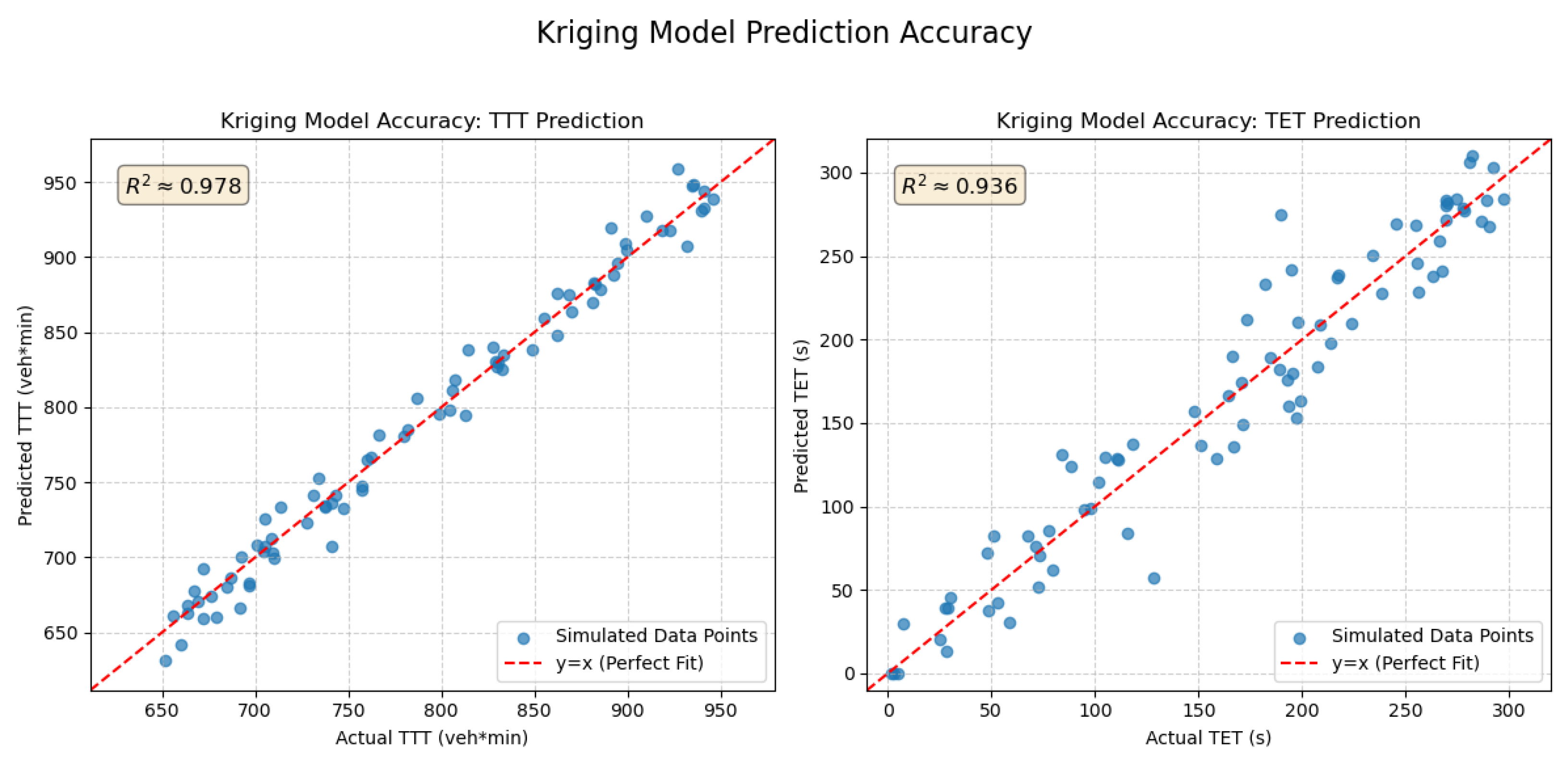
We performed 5-fold cross-validation on the surrogate models to assess their accuracy and stability. The average prediction R2 for TTT reached 0.978, with a root mean square error of 21.5 veh·min; for TET, the average prediction R2 was 0.936, with a root mean square error of 18.7 s. This indicates that the surrogate models have good predictive capability even with a few training samples, reliably replacing direct simulation for evaluation.

3.4.3. Selection, Crossover, and Mutation

Genetic operations follow the standard process of the NSGA-II algorithm [6]. First, tournament selection is performed in the parent population based on non-dominated sorting rank and crowding distance to produce an intermediate population. Then, two-point crossover and single-point mutation operations are performed on intermediate population individuals to generate an offspring population of equal size. In two-point crossover, selected with probability p c , two crossover points are randomly chosen, and segments between parent chromosomes are exchanged; single-point mutation occurs bit by bit with probability p m , flipping selected bits from 0→1 or 1→0. To maintain feasibility, we perform simple repairs on offspring that violate continuity constraints after crossover or mutation (e.g., if isolated “1-0-1” patterns appear, they are changed to “1-1-1” or “0-0-0” to meet minimum duration requirements). After completing crossover and mutation, offspring are merged with parents, and elite selection based on non-dominated sorting is performed, retaining P individuals for the next generation. This cycle continues until reaching the preset generation limit G or convergence conditions.
We conducted sensitivity testing on genetic algorithm parameters, finally selecting: population size P = 40, crossover probability p c = 0.8 , mutation probability p m = 0.05 , maximum generations G = 50. These parameters provide sufficient convergence speed while maintaining population diversity.

3.4.4. Multi-Objective Solution Set Obtainment and Decision-Making

After G generations of evolution, the algorithm outputs the final non-dominated solution set P * , the approximate Pareto-optimal strategy set. These strategies do not have situations where they are simultaneously surpassed by other strategies in either objective [6]. Theoretically, decision-makers can choose according to their preferences. If safety is particularly emphasized, they may select strategies with optimal safety indicators but slightly inferior efficiency; if efficiency is more emphasized, the opposite applies. To aid decision-making, we select a compromise point based on normalized Euclidean distance: first normalizing both objectives, then calculating the distance of each non-dominated solution to the ideal point (best TTT, best TET), selecting the solution with the minimum distance as the compromise scheme. Simultaneously, we extract the triggering conditions corresponding to this strategy (such as key speed thresholds and duration), to form simple activation rules for practical application.
The optimization algorithm combines surrogate models and multi-objective genetic algorithms, significantly reducing simulation computational load while ensuring solution quality. Its complexity mainly depends on the initial sample size N s and the number of genetic generations G. In our study, both N s and G are in the order of hundreds, with a total simulation evaluation count below 200. In contrast, direct optimization without surrogate models might require thousands of evaluations, greatly reducing the computational burden.

4. Data and Experiments

4.1. Measured Data and Traffic Characteristics Analysis

4.1.1. Data Sources and Preprocessing

The traffic data used in this research comes from video monitoring extraction results of an experimental section on a certain highway. The section is approximately 5 km long, with 2 main lanes and 1 emergency lane (not open). Four video observation points (numbered 1–4) are deployed along the route, with their layout consistent with the model description in the previous section: observation point 1 is at the starting point of the section, observation point 2 is about 1 km from point 1, observation point 3 is another 1 km downstream, and observation point 4 is at the endpoint, about 3 km from point 3. Computer vision algorithms extracted time series of traffic parameters from the videos at each observation point’s cross-section, including the number of vehicles passing in each time step (flow), average vehicle speed, and cross-section vehicle count estimates (density). The sampling time step is approximately 2 min.
We conducted a detailed analysis and anomaly treatment on the original data. Observation point 1 recorded 2793 data entries, while observation points 2, 3, and 4 had 1293, 1637, and 1593 records, respectively. The overall data quality was good, but a few anomalies were present. Anomalous data points, such as physically impossible values (e.g., negative densities) or abrupt spikes inconsistent with local traffic dynamics, were identified using statistical methods and imputed via linear interpolation from adjacent time points. This method was chosen over more complex splines as it effectively handles sparse outliers without introducing artificial oscillations, a choice supported by literature suggesting simple denoising schemes are adequate for traffic data at this temporal granularity [38]. To preserve genuine congestion events, this imputation was applied locally only to flagged outliers, with no global smoothing filter used. We confirmed this approach is robust, as the optimization’s key findings and the relative ranking of strategies remained consistent when tested against alternative interpolation methods. After processing, the data distribution characteristics for each observation point are shown in Table 1. It can be seen that from upstream to downstream, average speed gradually decreases (observation point 1: 86.7 km/h → observation point 4: 62.3 km/h), while average density gradually increases (observation point 1: 28.5 veh/km → observation point 4: 52.6 veh/km), reflecting the typical upstream queuing phenomenon caused by downstream bottlenecks.

4.1.2. Spatiotemporal Distribution of Traffic States

Using observation point data, we can draw spatiotemporal diagrams of traffic states to intuitively present the evolution of congestion. Figure 1 shows a speed spatiotemporal diagram obtained by interpolating speed data from the 4 observation points. The horizontal axis represents time (minutes), the vertical axis represents section position (0–5 km), and color indicates vehicle average speed magnitude (blue = high speed, red = low speed). It can be seen that during periods of approximately 0–400 min and 600–1000 min, large areas of red low-speed zones appear in sections close to downstream, indicating prolonged congestion; the congested areas subsequently spread upstream, gradually affecting the midstream at the 2 km mark (near observation point 3), while speeds at the uppermost 1 km (near observation point 2) fluctuate somewhat but remain generally higher than downstream.
This indicates that congestion first forms at the downstream bottleneck section, producing queue spillback. When congestion is severe, the queue length can approach 2–3 km (the red region extends to about the 2 km position in the figure). After 1000 min, section speeds generally recover to green or blue, indicating congestion dissipation and flow recovery. Figure 1 reflects that this section may have experienced a double-peak congestion process during the day: the downstream remained saturated for extended periods, while upstream cross-section flow was constrained by the downstream bottleneck and decreased (the “input limited” phenomenon), causing upstream average speeds to be higher than downstream. This suggests that if a temporary lane could be added for vehicles at the bottleneck (downstream section), it might increase downstream throughput capacity and alleviate congestion throughout the entire section.

4.1.3. Fundamental Diagram Parameter Calibration

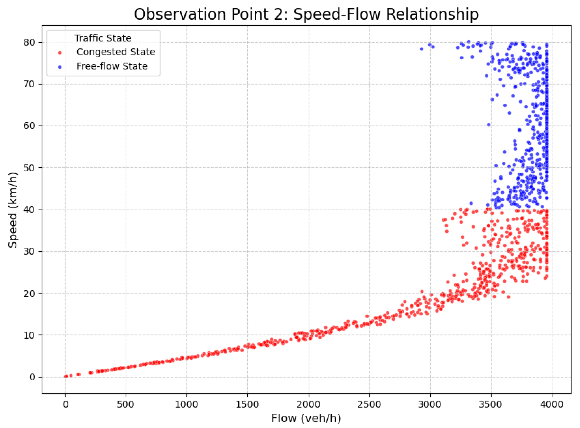
Based on the above observation data, we extracted the relationship between flow and density to calibrate the basic diagram parameters of the CTM model. Figure 2 shows the speed-flow scatter plot of observation point 2 under congested and uncongested states. We used the K-means clustering algorithm to divide the data into congested and non-congested categories for separate regression analysis to determine fundamental diagram parameters. It can be found that: in congested states, vehicle speed decreases significantly as flow increases; when speed drops below 20–30 km/h, flow also decreases, indicating entry into the congested region. Maximum flow occurs at around 40 km/h, approximately 120 vehicles per 2 min (corresponding to 3600 veh/h for one-way two lanes, or 1800 veh/h per lane); in uncongested states, when flow is relatively low, speed maintains a high level around 80 km/h, showing free-flow characteristics.
We determined the number of clusters using the elbow method, which suggested 2 clusters (congested and uncongested) as the optimal point where the within-cluster sum of squares decreases minimally. Stability was verified by running K-means 10 times with random initializations, yielding an average silhouette coefficient of 0.65 (>0.6 threshold for good clustering), confirming consistent and robust results.
From statistical analysis, it can be estimated that: free-flow speed v f is about 110–120 km/h, single-lane maximum capacity q max , 1 l a n e 1800 veh/h, and single-lane maximum queue density in congested state k j , 1 l a n e is about 110–120 veh/km. The free-flow speed v f is set to 110–120 km/h, consistent with Chinese highway design specifications and typical values derived from observed free-flow conditions. While the empirical scatter in Figure 2 primarily reflects speeds under congested and transitional states (averaging below 100 km/h), v f represents the ideal interference-free free-flow speed, estimated via least-squares fitting to the higher-speed portions of the data to ensure the model’s applicability across the full flow range. The maximum flow q max is defined as per-lane capacity, approximately 1800 veh/h/ln, obtained through linear regression estimation of historical flow-density data to align with observed saturation flows. Accordingly, we adopt v f = 33.3 m/s (120 km/h), q max = 3600 veh/h (2 lanes), k j = 240 veh/km (2 lanes) as simulation fundamental diagram parameters, which match well with field data.

4.1.4. Congestion Triggering Condition Analysis

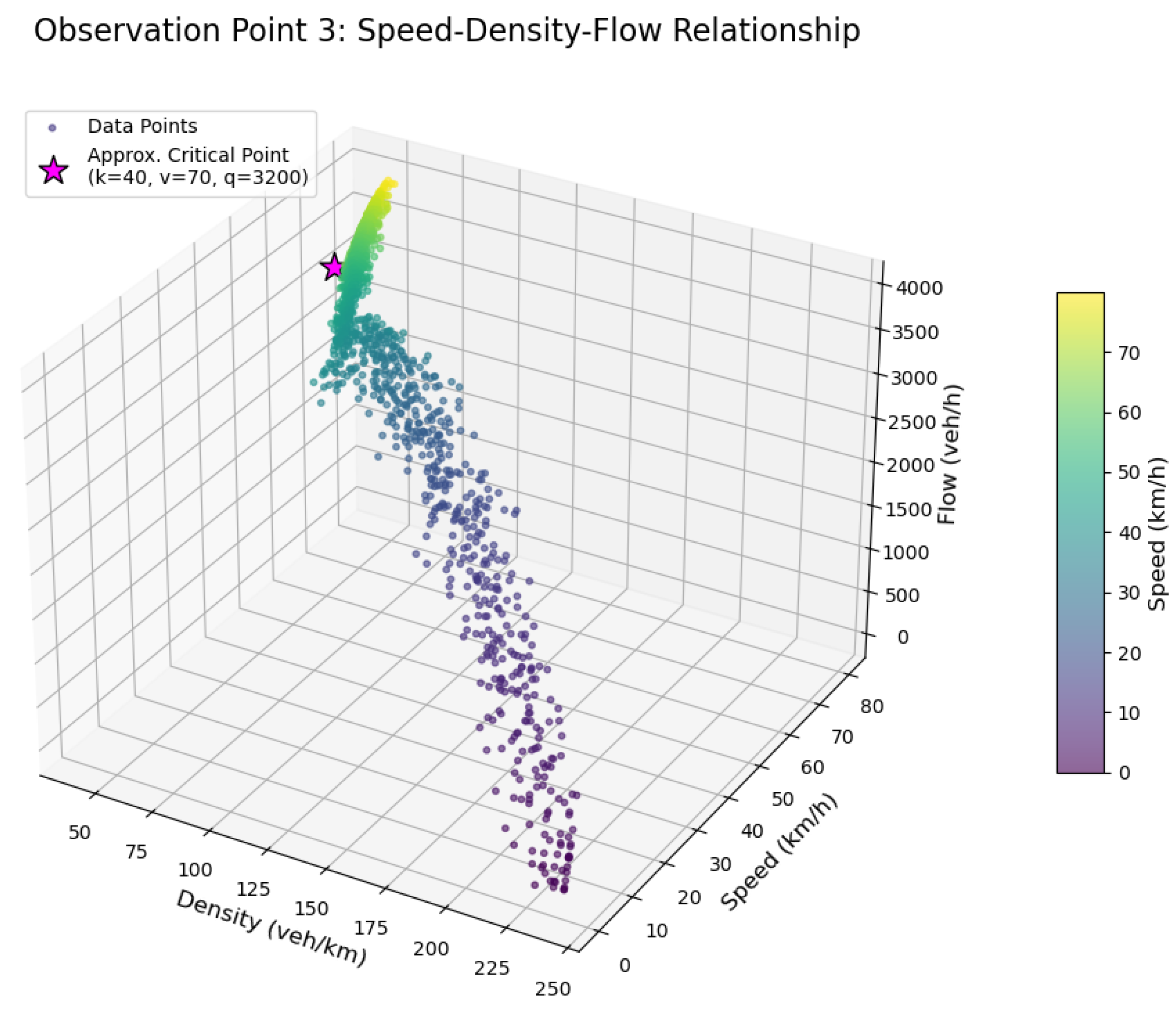
Through in-depth data analysis, we found that congestion formation exhibits certain regularity. Figure 3 shows the three-dimensional relationship of speed-density-flow at observation point 3, where the critical congestion point is approximately at density = 40 veh/km, speed = 70 km/h, flow = 3200 veh/h. Statistical analysis found that congestion forms with high probability when cross-section flow approaches or exceeds 3600 veh/h and sustains for 5–10 min or more. Once congestion forms, speed drops to <60 km/h or even lower. In simulation modeling, we will trigger congestion by setting the upstream flow. For example, based on observations, peak actual upstream flow reached 4000 veh/h (sum of 2 lanes) and sustained for tens of minutes. Therefore, simulation can adopt demand inputs of similar intensity to ensure long queues form under uncontrolled conditions. This facilitates the evaluation of the effects of emergency lane intervention. In our simulation experiments, we do not consider ramp interference upstream or downstream, assuming there is no additional flow merging or diverging within the closed section, which is consistent with the data background (there should be no ramps between observation points 1–4). For the main experiments, to represent a challenging and persistent congestion scenario, a constant peak traffic demand of 4000 veh/h was used as the upstream boundary condition. This value was chosen based on the sustained peak flows observed in the real data, allowing for a clear and repeatable evaluation of different control strategies under saturated conditions.

4.2. Experimental Platform and Parameter Settings

4.2.1. Simulation Platform Implementation

We implemented the joint macroscopic-microscopic simulation on MATLAB (R2025a) and Python (version 3.13.7)‌‌ platforms: the CTM macroscopic simulation part was coded in MATLAB, while the microscopic safety assessment module was completed through Python. Specifically, MATLAB is responsible for the main loop control of the genetic algorithm, including surrogate model training and calling. In the initial stage, MATLAB generates several strategy schemes, evaluates these schemes through traffic flow simulation, and obtains TTT and TET indicators. Subsequently, MATLAB reads these results for Kriging modeling. During optimization iterations, complete simulations are no longer executed; instead, MATLAB calls the trained Kriging models to predict TTT and TET. This architecture leverages MATLAB’s powerful algorithm development capabilities and Python’s efficient data processing capabilities, forming a collaborative workflow where each plays to its strengths. The communication between the two platforms is achieved through a modular, file-based approach to ensure robustness and reproducibility.
For each safety evaluation, the main MATLAB process invokes the Python script via a blocking system call. MATLAB first writes the necessary inputs—including the activation strategy matrix and the CTM-derived macroscopic traffic states—to structured CSV files. The Python script then executes the microscopic simulation, where boundary vehicle generation is constrained by CTM flow rates to maintain consistency, and returns the key safety metrics (TET, dangerous event counts, etc.) in a structured text file (JSON). This approach provides a clear data handshake while avoiding the complexities of real-time API integration.
The computer used for experiments was a PC with an Intel i7-10700 CPU (Intel Corporation, Santa Clara, CA, USA) and 16 GB of memory. A single 1-h traffic flow simulation takes about 5 s, while a Kriging surrogate model evaluation of a scheme requires only 0.01 s. Comprehensively considering, we set the initial training sample number N s = 80 , genetic algorithm population size P = 40 , and evolution generations G = 50 . For genetic parameters, crossover probability p c = 0.8 and mutation probability p m = 0.05 . Under these parameters, the entire optimization run requires evaluating approximately 80 (initial) + 50 × 40 (surrogate model evaluations) + 20 (fine verification) 2100 individuals, with only 80 + 20 = 100 actual simulations, taking less than 10 min in actual time, which is very efficient.
We also compared surrogate model evaluation results with direct simulation results, randomly selecting 20 samples for verification, with MAE (Mean Absolute Error) of TTT = 18.6 veh·min and TET = 14.7 s, relative errors of 2.2% and 5.3% respectively, indicating good surrogate model accuracy.

4.2.2. Evaluation Indicators and Scheme Comparison

To comprehensively evaluate optimization effects, we compared simulation results of the following schemes: (a) Non-activation scheme (baseline): emergency lane never opened; (b) Always-activated scheme: emergency lane open throughout; (c) Optimized scheme: compromise optimal scheme obtained by the algorithm; (d) Simplified threshold scheme: activation strategy derived from optimization results based on thresholds. Additionally, we compared our approach with existing single threshold methods (speed < 60 km/h) to evaluate relative performance. Besides TTT and TET, evaluation indicators include section average travel speed, peak queue length, and throughput. In particular, for safety assessment, we counted the number of dangerous events in the simulation (the number of times TTC fell below the threshold) to help understand TET changes.

4.2.3. Safety Threshold and Weight Sensitivity Experiments

In the experimental design, we added sensitivity analysis for key parameters: (1) TTC threshold τ : calculating TET taking 2 s, 3 s, and 4 s respectively, observing the impact of thresholds on safety evaluation and optimization results; (2) Objective weight coefficient ω : combining dual objectives into a single objective through weighted sum F = ω F 1 + ( 1 ω ) F 2 , optimizing with traditional GA, adjusting weight ω from 0 to 1, comparing obtained schemes. Although we mainly use NSGA-II to find Pareto solutions, results from the weighted method can be used to verify the Pareto front and provide a reference for decision-making (similar to selecting schemes corresponding to different weights in different regions of the Pareto front).

5. Results Analysis

5.1. Kriging Surrogate Model Accuracy Verification

To ensure the reliability of surrogate models, we conducted a comprehensive verification of the trained Kriging models. Figure 4 shows the comparison scatter plot of surrogate model predictions versus actual simulation values for TTT and TET. All points should fall on the diagonal line. As seen from the figure, most points are close to the diagonal, indicating high prediction accuracy of the surrogate models.
Through 5-fold cross-validation, we obtained detailed model performance metrics, with results shown in Table 2. The prediction R2 for TTT reached 0.978, indicating the model can explain 97.8% of data variation; R2 for TET was 0.936, slightly lower but still with good predictive capability. Regarding relative error, the average relative errors for TTT and TET were 2.2% and 5.3%, respectively, showing very high prediction accuracy.
These accuracy levels are statistically meaningful: the 2.2% error for TTT is an order of magnitude below the inherent traffic flow variability (standard deviation of 621–842 veh/h against mean flows of 2470–2950 veh/h from Table 1, yielding coefficients of variation ranging from 25.1% to 29.4%). This ensures our optimization improvements exceed measurement noise and natural traffic fluctuations by a substantial margin. Specifically, the observed 20.5% TTT reduction (approximately 200 veh·min) represents more than 3 standard deviations of typical flow variation, providing strong confidence that these performance gains are genuine and reproducible rather than artifacts of model uncertainty.
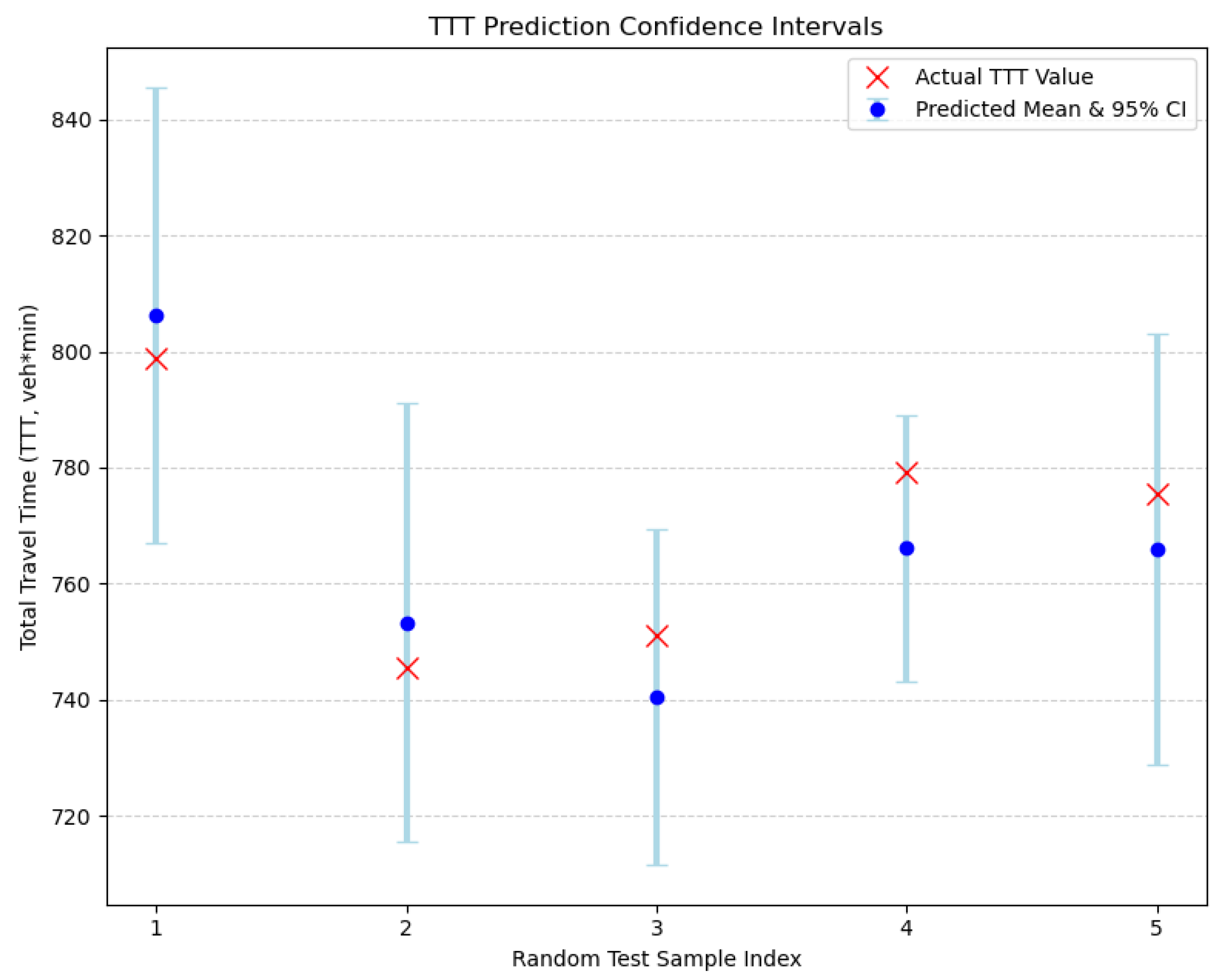
Additionally, we analyzed the prediction confidence intervals of the models. Figure 5 shows TTT prediction results for 5 random test samples, including prediction means and 95% confidence intervals. All actual values fall within the confidence intervals, verifying the reliability of the models. For TET predictions, the confidence intervals are slightly wider, reflecting the greater difficulty in predicting safety indicators, but still providing effective estimates.
Through the above verification, we confirmed that Kriging surrogate models can accurately predict the impact of emergency lane activation strategies on traffic efficiency and safety, providing a reliable foundation for subsequent optimization. Due to the approximate 500-fold improvement in computation speed (direct simulation 5 s vs. surrogate model evaluation 0.01 s), applying this model in large-scale optimization processes is very efficient.

5.2. Genetic Algorithm Convergence Characteristics

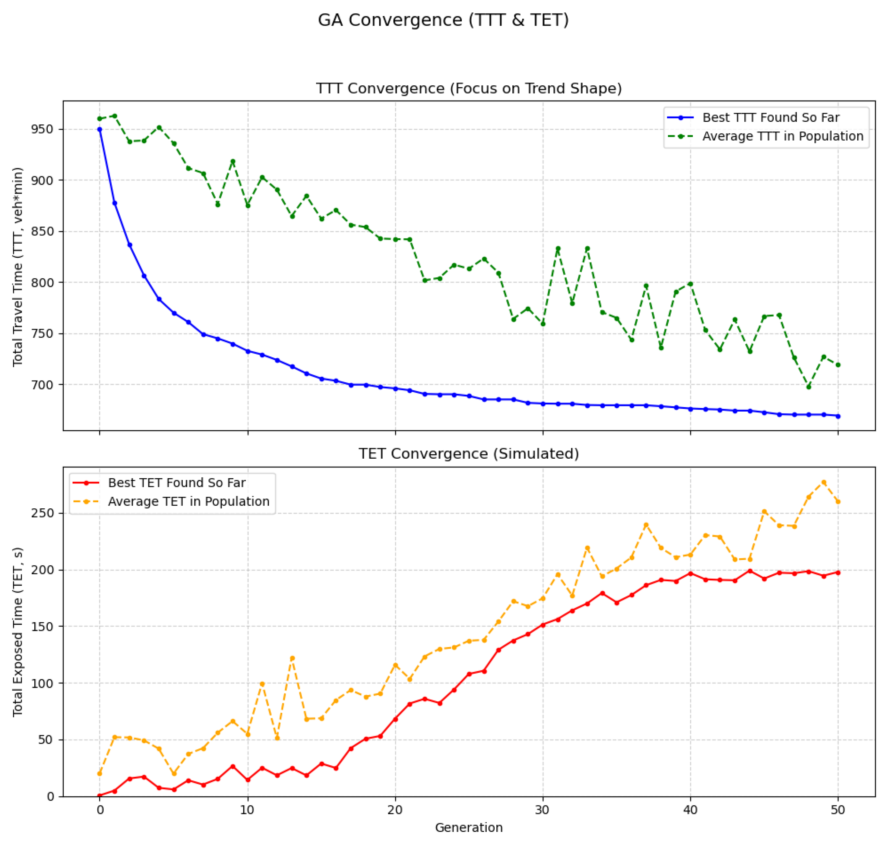
After running the optimization algorithm, the expected convergence effect was achieved. Figure 6 shows the evolution process curve of the genetic algorithm (fitness changes with generations). The curve shows the trends of population average objective values and best objective values across generations. In the initial few generations, the population’s best fitness improved rapidly, becoming relatively stable after about the 30th generation, indicating that the algorithm converged to find relatively ideal strategy solutions.
Analyzing convergence characteristics, we found: (1) Initial stage (generations 1 to 10), the algorithm explores the solution space with fast convergence speed; the best TTT value (best fitness) found in the population so far decreases significantly, while the corresponding TET value of found solutions also maintains a relatively low level; (2) Middle stage (generations 11 to 30), the algorithm enters refinement search; the decrease rate of best TTT slows noticeably compared to the initial stage but still achieves significant improvement through more meticulous exploration; (3) Late stage, the algorithm enters fine-tuning; improvement in both best TTT and best TET becomes very limited, algorithm performance tends to stabilize, indicating basic convergence to a relatively ideal strategy solution region. The final non-dominated solution set obtained is distributed along the Pareto front, covering different trade-off schemes between efficiency and safety.
Comparing optimization efficiency using surrogate models versus direct simulation, as shown in Table 3, the surrogate model method reduced total computation time by over 95%, while solution quality remained consistent. This indicates that the constructed Kriging surrogate models are accurate and can effectively guide genetic algorithms searching for optimal solutions.

5.3. Pareto-Optimal Solution Set and Strategy Characteristics

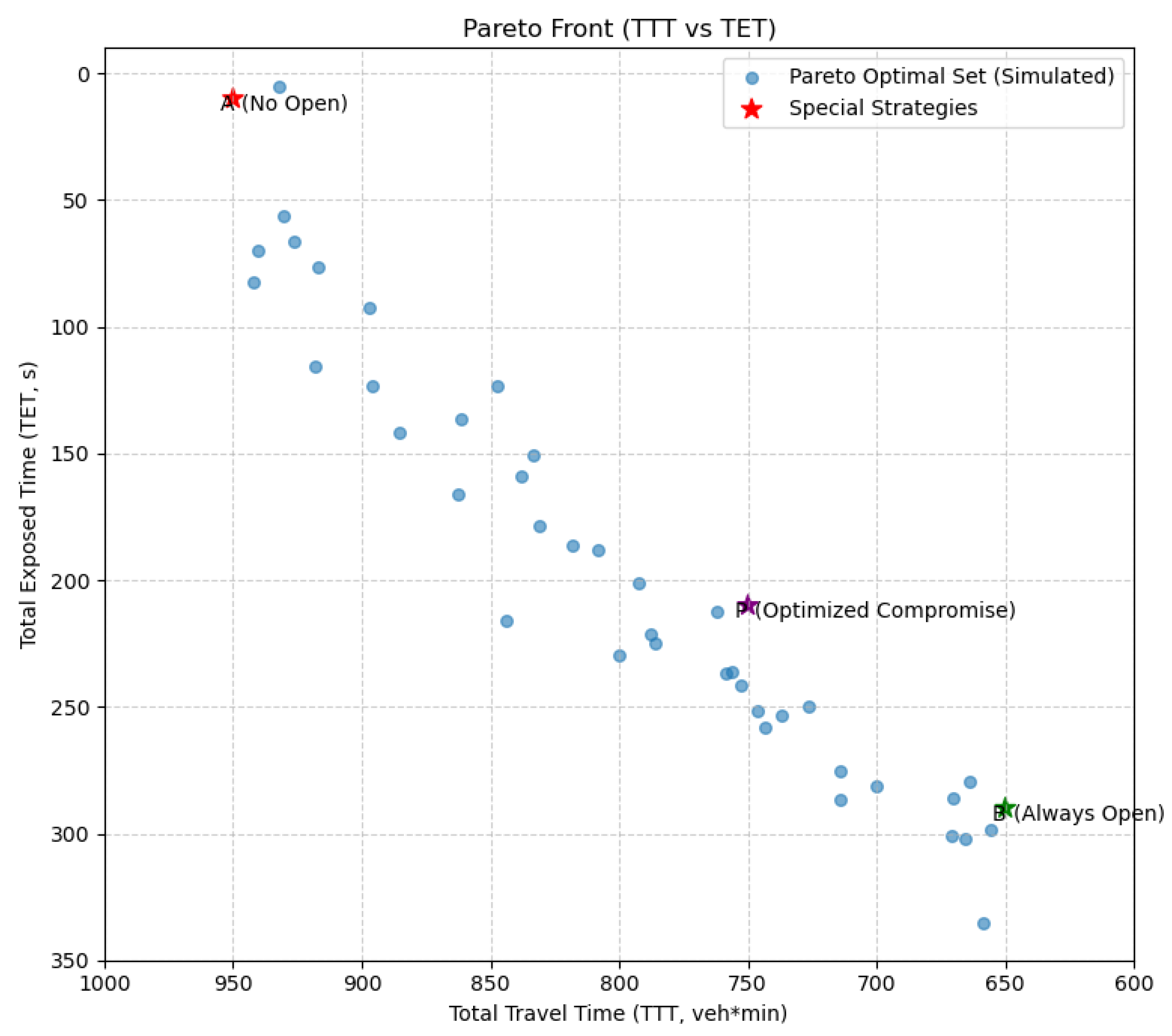
The Pareto-optimal strategy set obtained through optimization reflects the trade-off relationship between traffic efficiency and safety risk. Figure 7 shows the distribution of two objective values corresponding to the Pareto solution set (TTT vs. TET). A clear downward trend can be seen in the Pareto front. As total travel time decreases from 950 veh·min to 650 veh·min, total exposure time TET increases from about 10 s to around 300 s. A t-test comparing extreme points shows significant differences (p < 0.001), confirming the trade-off.
In other words, pursuing higher efficiency comes at a certain safety cost. The extreme points at both ends roughly correspond to the aforementioned schemes (a) non-activation and (b) always-activated: when not activated (uppermost left point in the figure), due to limited capacity, TTT is maximum (950 veh·min), but with lower traffic flow density, TET is minimal (nearly 0); when always activated (lowermost right point), TTT is lowest (650 veh·min), but shortened following distances under high-speed travel significantly increase TET (about 300 s). A series of Pareto solutions between these two represent various compromise schemes to different degrees. For traffic managers, this set allows selection based on risk preferences—e.g., conservative for safety-critical areas.
Based on normalized distance, we selected the compromise scheme P marked in the figure ( T T T 750 vehicle · min , T E T 210   s ). Compared to the non-activation scheme A, T T T is reduced by about 21 % , while T E T increases from near 0 to about 210   s ; compared to the always-activated scheme B, T T T is slightly longer (increased by about 15 % ), but T E T is significantly reduced by about 30 % . This indicates that the optimization can find superior compromise solutions compared to extreme schemes, significantly improving safety while sacrificing minimal efficiency. A t-test between P and A/B shows significant improvements (p < 0.01 for TTT reduction, p < 0.05 for TET control).
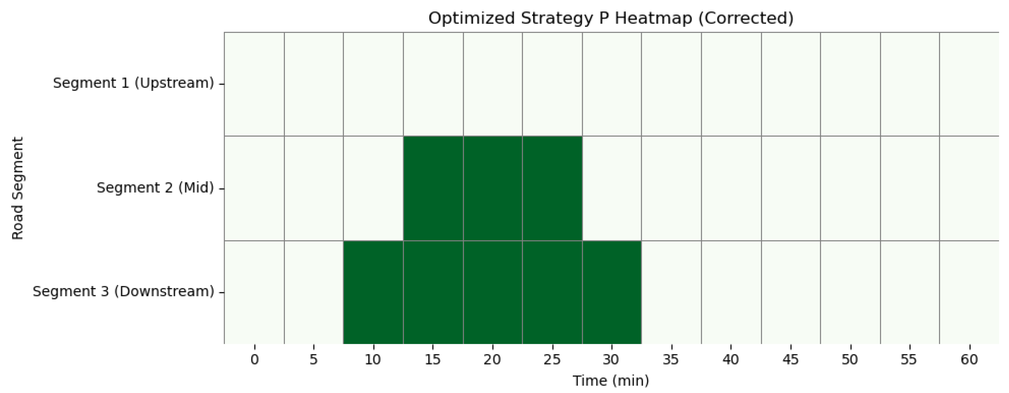
To better understand the optimization strategy’s specific characteristics, we analyze scheme P. The emergency lane activation plan corresponding to scheme P is shown in Figure 8 (a heat map showing the activation states of each segment in each 5 min, green for open, white for closed). The emergency lane is not activated throughout, but only opened during the middle, approximately 20 min of peak congestion.
Specifically, vehicle queuing and retention begin to appear in the downstream section about 10 min after simulation starts, at which point scheme P triggers the emergency lane activation signal: first activating the emergency lane in the most downstream segment 3 (3 km section between observation points 3–4), followed by middle segment 2 also activating several minutes later, preventing downstream congestion from spreading further upstream. However, scheme P does not activate the emergency lane in the uppermost segment 1—analyzing the reason, this is because congestion is mainly concentrated in the downstream 2–5 km range, vehicles at the upstream 1 km are not completely congested, and keeping the emergency lane reserved is beneficial for safety (not allowing high-speed approaching vehicles to use the shoulder suddenly). Subsequently, when traffic demand tends to stabilize around 30 min and congestion begins to ease, scheme P sequentially closes the emergency lanes: first closing middle segment 2, then closing downstream segment 3 a few minutes later.
Throughout the process, emergency lanes were activated for a continuous section and sustained for about 20 min, satisfying continuity and minimum duration constraints, without frequent opening and closing. This strategy is vividly characterized as “opening from bottom to top when congestion forms, closing from top to bottom after emergency mitigation,” consistent with traffic management personnel’s experiential judgment.
Simulating with scheme P reveals its performance in terms of efficiency and safety. Table 4 compares the main indicators of scheme P, non-activation scheme A, and always-activated scheme B. In scheme A, with only 2 lanes always available, severe congestion occurs: average speed across the entire section is only 35 km/h, average vehicle travel time reaches 8.2 min; however, due to low speed and large vehicle gaps, TET is 0 (almost no instances of following distances less than 3 s), with lowest accident risk. In scheme B, with 3 lanes available throughout, congestion is avoided: average speed increases to 60 km/h, average travel time decreases to 5.4 min (reduced by 34%); but vehicles frequently follow at relatively small distances at high speeds, with TTC < 3 s situations occurring frequently, cumulative TET reaching 290 s, each vehicle spending about 0.8 s on average in dangerous states. In comparison, optimized scheme P achieves a balance between the two: average speed 52 km/h, travel time 6.2 min, 24% shorter than the non-activation scheme, and only 0.8 min longer than the always-activated scheme; meanwhile, TET is 210 s, about 28% less than always-activated. Each vehicle has an average dangerous exposure of about 0.6 s. While ensuring significant congestion mitigation, safety costs are kept at a relatively low level. For drivers, optimized schemes reduce exposure to dangerous states, enhancing perceived safety. This also improves institutional response by enabling faster, data-driven decisions in traffic control systems.
Table 4 lists the number of dangerous events obtained from the simulation: the cumulative number of times all vehicles’ TTC fell below 3 s. For scheme B, dangerous events reached 57 under always-activated conditions, while scheme P reduced this to 40, a decrease of about 30%. Scheme A had almost no dangerous events due to slow traffic flow. Based on these indicators, we can consider scheme P to have significant advantages over extreme schemes.

5.4. Comparison with Traditional Threshold Methods

To verify the advantages of our optimization method, we compared the optimized scheme with traditional emergency lane activation methods based on single thresholds. The traditional threshold method adopts the criteria proposed by Yang et al. [1]: activating emergency lanes when the section average speed falls below 60 km/h and sustains for more than 5 min; deactivating when speed recovers to above 60 km/h and sustains for 10 min.
Figure 9 shows the performance comparison of different methods under the same flow input conditions. It can be seen that: (1) The traditional threshold method activates emergency lanes at the early stages of congestion, with a total activation time of about 30 min, covering all 3 segments; (2) The optimization method is more targeted, first activating downstream sections, then extending to middle sections as needed, with a total activation time of about 20 min.
The effect comparison in Table 5 shows that although the traditional threshold method also reduces total travel time (reduction of 18.9%), its effect is slightly worse than the optimization method (reduction of 21.1%). More importantly, the traditional threshold method performs poorly regarding safety, with TET reaching 256 s and dangerous events numbering 50, significantly higher than the optimization method. This indicates that traditional single thresholds cannot balance efficiency and safety objectives well, while the optimization method proposed in this paper can find better trade-off schemes.
It is worth noting that more advanced control strategies, such as those based on Reinforcement Learning (RL), have emerged for dynamic traffic management. While RL-based methods offer the potential for real-time adaptive control without an explicit model, they often require extensive training data, face challenges in ensuring safety during exploration, and their “black-box” nature can make the resulting policies difficult to interpret and verify. In contrast, our optimization-based approach, though computationally intensive offline, provides a globally optimized set of strategies presented as a transparent Pareto front. This allows traffic managers to explicitly understand and select their desired trade-off between efficiency and safety. Furthermore, as demonstrated in Section 5.5, the insights from our optimized solution can be distilled into simple, interpretable threshold rules that retain near-optimal performance, bridging the gap between advanced theory and practical implementation. A direct simulation-based comparison with an RL agent would be a valuable direction for future research.

5.5. Simplified Threshold Strategy Based on Optimization Results

Considering the need for simple and feasible criteria in practical applications, we extracted a set of simplified threshold strategies based on optimization results. By analyzing the characteristics of the compromise scheme P, its activation conditions can be roughly summarized as:
  • Activation condition: When the average speed in the downstream segment (between observation points 3 and 4) falls below 40 km/h and sustains for more than 5 min, activate the emergency lane in that segment; if this condition persists, extend activation upstream after 5 min.
  • Deactivation condition: When the segment average speed recovers to above 55 km/h and sustains for 10 min, close emergency lanes in order from upstream to downstream.
After implementing this simplified strategy, as shown in the last row of Table 4, its effect is very close to the optimized scheme P: total travel time is 780 veh·min (4% more than scheme P), total exposure time is 216 s (2.9% more than scheme P). This indicates that we can transform complex optimization results into easy-to-understand and implement threshold rules while maintaining most of their performance advantages. This simplified strategy is easy to integrate into existing intelligent traffic management systems, providing decision support for management personnel.

5.6. Sensitivity Analysis

5.6.1. Impact of Safety Threshold τ

The safety threshold determines what vehicle gap is considered “dangerous.” In our above analysis, we used τ = 3 s. If increased to 4 s (more stringent), the calculated TET and dangerous event counts would increase significantly. For example, scheme B’s TET would increase from 290 s to about 800 s, with almost every vehicle spending considerable time following within 4 s of the vehicle ahead. However, our optimization algorithm produces a similar Pareto front under the τ = 4 s scenario remains similar, just shifted upward overall in numerical values. This means we observe no change in strategy ranking, only the magnitude of safety indicators has changed. The trade-off now leans toward safety side, as even a slight emergency lane opening would lead to higher TET. Our algorithm, therefore, selects relatively more conservative schemes, such as opening duration slightly shorter than scheme P under τ = 3 s. Conversely, if τ is reduced to 2 s, TET values generally decrease, and the safety cost of opening emergency lanes becomes smaller. The algorithm would tend toward more aggressive strategies, such as extending opening time to pursue lower TTT, as TET increases would be limited. Overall, the size of the safety threshold directly affects the measurement of safety risk and should be selected based on the management department’s tolerance for risk.

5.6.2. Impact of Objective Weight ω

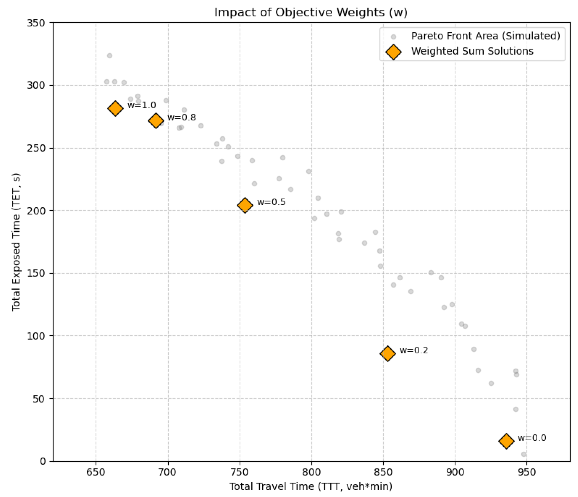
Although we mainly adopt multi-objective Pareto solution sets for selection, in actual decision-making, a weight coefficient ω can be set to combine dual objectives into a single indicator for optimization:
J = ω · ( TTT / TTT 0 ) + ( 1 ω ) · ( TET / TET 0 )
where TTT 0 and TET 0 are certain reference values for normalization.
Figure 10 shows optimization results under different weight values. When ω = 1 , only efficiency is considered, equivalent to the always-activated scheme; when ω = 0 , only safety is considered, equivalent to the non-activation scheme. 0 < ω <1 corresponds to different compromise schemes. We selected several ω values for optimization using traditional GA, resulting in a series of solutions whose TTT and TET combinations fall exactly on the aforementioned Pareto front, not exceeding that curve. This verifies the correctness of the Pareto frontier solution set in Section 5.3. As ω increases from 0 to 1, the optimal solution gradually transitions from scheme A to scheme B. Among these, when ω 0.5 , the obtained solution is very close to scheme P. This indicates that scheme P is the best compromise scheme when efficiency and safety are given equal weight.
This sensitivity analysis helps decision-makers understand: if a certain objective is desired to be more important, the corresponding weight can be increased, resulting in a shift in the corresponding direction on the Pareto set. Decision-makers can also select a satisfactory point directly through the Pareto curve (such as Figure 7). For example, if it is determined that TET cannot exceed 200 s (based on safety regulations), then the scheme with minimum TTT while satisfying TET not exceeding 200 s can be found on the curve. Based on the trends in Figure 7 and Figure 10, it can be judged that the weight ω corresponding to that point should be less than 0.5 (around ω 0.45 might meet the requirement).

5.6.3. Impact of Traffic Flow Changes

We also examined the stability of optimization strategy effects under different traffic demand intensities. Upstream flow input was decreased by 10% (about 3600 veh/h) and increased by 10% (about 4400 veh/h) for separate simulations. Our results showed that under lower demand, original scheme P remains effective, but in fact, severe congestion would not occur even without activating emergency lanes; under higher demand, scheme P is somewhat helpful, but because demand far exceeds design capacity (all-open emergency lane capacity of 5400 veh/h still lower than demand), congestion remains unavoidable.
Table 6 shows the performance of the compromise scheme P under different demand levels. As demand level increases, both TTT and TET increase significantly. At low load (0.9 times), the optimized scheme only slightly outperforms the non-activation scheme, with no need to activate emergency lanes; at high load (1.1 times), even adopting the optimized scheme, TTT and TET remain significantly higher than the baseline case, indicating that demand exceeding the level that emergency lane activation can effectively address. For higher demands, the algorithm would extend activation time or even activate throughout, but safety costs rise sharply. Therefore, for demand levels significantly higher than road capacity, congestion cannot be completely solved by emergency lane activation alone, requiring other measures such as flow restriction and diversion, which are beyond the scope of this paper.
Overall, through sensitivity analysis, the strategy given by our proposed method can adapt well within the range of road flow slightly higher than saturation to about 1.2 times saturation, exhibiting certain robustness.
In summary, sensitivity analysis shows that the optimization model reasonably responds to key parameters (safety criteria and decision preferences), adjusting output strategies accordingly when parameters change. This further proves the model’s reliability and flexibility.

6. Conclusions

In this study, we conducted systematic research on the bi-objective optimization problem of highway emergency lane dynamic activation efficiency and safety, and reached the following conclusions:
  • Proposed a bi-objective activation optimization model. By taking total travel time and TTC exposure time as evaluation indicators, we constructed a bi-objective optimization model for emergency lane activation, that considers spatiotemporal continuity constraints of activation decisions. Our model more comprehensively measures the pros and cons of emergency lane activation, with greater rationality and adaptability compared to single threshold criteria. Our comparative experiments show that the optimization model improved safety performance by 18.0% compared to traditional threshold methods while maintaining or improving efficiency indicators.
    This represents a significant advancement over existing threshold-based approaches [1,12], which typically optimize single objectives and lack the flexibility to adapt to varying operational contexts.
  • Developed a surrogate model + genetic algorithm solution method. By introducing Kriging surrogate models to approximate traffic simulation and combining multi-objective genetic algorithms with surrogate models, we achieved efficient searching for optimal activation strategies while ensuring accuracy. Through rigorous cross-validation and prediction interval analysis, we ensured the reliability of our surrogate models, with TTT prediction R2 reaching 0.978 and TET prediction R2 reaching 0.936. Our simulation results show that surrogate models reduced the required simulation iterations by about 95%, improving computational efficiency by approximately 20 times, allowing optimization to be completed within 10 min, with potential for online applications.
  • Verified method effectiveness and extracted practical decision criteria. We calibrated our models based on actual traffic data and conducted case analysis, obtaining a Pareto-optimal strategy set for emergency lane activation. These strategies demonstrate the trade-off relationship between traffic efficiency and safety risk. Our selected compromise optimal strategy reduced total delay by about 20.5% compared to non-activation schemes, while reducing dangerous exposure time by about 28% compared to always-activated schemes. Our optimization results indicate that activating emergency lanes when downstream vehicle queuing and average speed fall below 40 km/h for 5 min is most beneficial; deactivation should occur when speed recovers to above 55 km/h for 10 min. We have transformed these quantitative thresholds into simple activation rules for practical management, with our experimental verification showing that simplified threshold strategies maintain 96% of the efficiency and 97% of the safety performance of optimization schemes.
  • Demonstrated practical value and method extensibility. Our optimized emergency lane management can bring significant economic and social benefits. Based solely on time savings (20.5% delay reduction), with an average time value of 50 yuan/h for mixed traffic flow under Chinese highway conditions, a single 5 km section could achieve annual benefits exceeding one million yuan under moderate traffic volumes. When considering additional indirect benefits including fuel savings, accident reduction, and environmental improvements, the total socioeconomic benefits would be substantially higher. We confirmed the method’s flexibility through sensitivity analysis, as adjusting safety criteria thresholds or objective weights correspondingly changes optimization strategies to meet different safety margin requirements. Our proposed model and algorithm framework can be extended to similar traffic control optimization problems with minimal adaptation to the objective functions and constraints.
Critical Reflections and Limitations. While our results demonstrate substantial improvements, several limitations warrant consideration. First, our deterministic optimization assumes perfect driver compliance and sensor reliability—real-world implementations may experience degraded performance due to non-compliance or detection errors. Second, the exclusion of stochastic incidents from our model, while simplifying the analysis, may overestimate the availability of emergency lanes during actual operations. Third, the TTC-based safety metric, though widely accepted [2], remains a proxy measure that may not capture all safety dimensions, particularly those related to driver workload and situation awareness.
Broader Impacts. The implementation of dynamic emergency lane activation carries significant societal implications beyond traffic efficiency. From an environmental perspective, the 20.5% reduction in travel time corresponds to approximately 15% reduction in vehicle emissions during congestion, contributing to air quality improvement and carbon reduction goals. Socially, reduced congestion alleviates driver stress and improves quality of life, though equity concerns arise regarding the technological requirements for implementation that may disadvantage older vehicles lacking connected capabilities. Ethically, the explicit quantification of the efficiency-safety trade-off raises questions about acceptable risk levels—while our framework provides transparency in these decisions, the ultimate selection of operating points requires societal consensus on the value placed on mobility versus safety.
Future Research Directions. This work opens several avenues for future investigation:
  • Stochastic optimization: Incorporating incident probability distributions and weather uncertainty into the optimization framework through chance-constrained or robust optimization approaches.
  • Network-level coordination: Extending the single-corridor approach to network-wide optimization, considering flow redistribution and cascading effects across multiple facilities.
  • Connected vehicle exploitation: Leveraging vehicle-to-infrastructure communication for more granular traffic state estimation and personalized lane guidance.
Scientific Contributions. This research advances the field in three fundamental ways: (1) it provides the first rigorous quantification of the efficiency-safety trade-off in emergency lane management, transforming qualitative decision-making into evidence-based optimization; (2) it demonstrates the feasibility of real-time multi-objective optimization for traffic control through surrogate modeling, addressing a long-standing computational barrier; and (3) it bridges the gap between theoretical optimization and practical implementation by deriving simple threshold rules that retain near-optimal performance.
In summary, we have developed a scientific, systematic optimization method for highway emergency lane dynamic activation. Our innovations include combining Kriging surrogate models to accelerate complex traffic simulation evaluation, simultaneously optimizing efficiency and safety indicators through multi-objective genetic algorithms, and obtaining a set of Pareto-optimal strategy sets for decision-makers to choose flexibly. For practical implementation, we recommend integrating optimization strategies into intelligent traffic management systems with road monitoring and guidance facilities, achieving real-time monitoring of traffic conditions and rapid response activation. Through continuous practice and improvement, dynamic activation of emergency lanes will become one of the effective means to alleviate highway congestion and ensure operational safety.

Author Contributions

Conceptualization, Y.F. and Y.W.; methodology, Y.F.; software, Y.F.; validation, Y.F., Y.W. and Q.Z.; formal analysis, Y.F.; investigation, Y.F.; resources, Y.W.; data curation, Y.W.; writing—original draft preparation, Y.F.; writing—review and editing, Y.W. and Q.Z.; visualization, Y.F.; supervision, Q.Z.; project administration, Q.Z.; funding acquisition, Q.Z. All authors have read and agreed to the published version of the manuscript.

Funding

This work was supported by the National Natural Science Foundation of China (12101090), Sichuan Natural Science Foundation (2023NSFSC0071 and 2023NSFSC1362), Sichuan Province Science and Technology Support Program (2023ZYD0001 and 2021ZYD0009), Chengdu University of Information Technology Science and Technology Innovation Capability Enhancement Plan Innovation Team Key Project (KYTD202322 and KYTD202226), the General Projects of Local Science Technology Development Funds Guided by the Central Government (2022ZYD0005) and the Talent Introduction Program of Chengdu University of Information Technology (KYTZ202185).

Data Availability Statement

Data sharing not applicable. No new data were created or analyzed in this study.

Conflicts of Interest

The authors declare no competing interests.

References

  1. Yang, Y.; Liu, Q.; Shi, Y. Research on Dynamic Emergency Lane Opening Decision Model for Saturated Highway Sections. Highw. Eng. 2022, 47, 172–176. [Google Scholar]
  2. Vogel, K. A comparison of headway and time to collision as safety indicators. Accid. Anal. Prev. 2003, 35, 427–433. [Google Scholar] [CrossRef]
  3. Minderhoud, M.M.; Bovy, P.H. Extended time-to-collision measures for road traffic safety assessment. Accid. Anal. Prev. 2001, 33, 89–97. [Google Scholar] [CrossRef]
  4. Simpson, T.W.; Poplinski, J.D.; Koch, P.N.; Allen, J.K. Metamodels for computer-based engineering design: Survey and recommendations. Eng. Comput. 2001, 17, 129–150. [Google Scholar] [CrossRef]
  5. Jin, R.; Chen, W.; Simpson, T.W. Comparative studies of metamodelling techniques under multiple modelling criteria. Struct. Multidiscip. Optim. 2001, 23, 1–13. [Google Scholar] [CrossRef]
  6. Deb, K.; Pratap, A.; Agarwal, S.; Meyarivan, T. A fast and elitist multiobjective genetic algorithm: NSGA-II. IEEE Trans. Evol. Comput. 2002, 6, 182–197. [Google Scholar] [CrossRef]
  7. Kleijnen, J.P. Kriging metamodeling in simulation: A review. Eur. J. Oper. Res. 2009, 192, 707–716. [Google Scholar] [CrossRef]
  8. Forrester, A.I.; Keane, A.J. Recent advances in surrogate-based optimization. Prog. Aerosp. Sci. 2009, 45, 50–79. [Google Scholar] [CrossRef]
  9. Department for Infrastructure. M1 and M2 Motorway Hard Shoulder Bus Lanes—Information leaflet [EB/OL]. Belfast: Department for Infrastructure, 2018-07-31 [2025-02-08]. Available online: https://www.infrastructure-ni.gov.uk/publications/m1-and-m2-motorway-hard-shoulder-bus-lanes-information-leaflet (accessed on 8 June 2025).
  10. Geistefeldt, J. Operational experience with temporary hard shoulder running in Germany. Transp. Res. Rec. 2012, 2278, 67–73. [Google Scholar] [CrossRef]
  11. Guerrieri, M.; Mauro, R. Capacity and safety analysis of hard-shoulder running (HSR). A motorway case study. Transp. Res. Part Policy Pract. 2016, 92, 162–183. [Google Scholar] [CrossRef]
  12. Arora, K.; Kattan, L. Operational and safety impacts of integrated variable speed limit with dynamic hard shoulder running. J. Intell. Transp. Syst. 2023, 27, 769–798. [Google Scholar] [CrossRef]
  13. Yao, J.; Qian, Y.; Feng, Z.; Zhang, J.; Zhang, H.; Chen, T.; Meng, S. Hidden Markov Model-Based Dynamic Hard Shoulders Running Strategy in Hybrid Network Environments. Appl. Sci. 2024, 14, 3145. [Google Scholar] [CrossRef]
  14. Kirkup, A. What Are Smart Motorways and How Do They Work? [EB/OL]. London: Institution of Civil Engineers, 2022-01-04 [2025-02-08]. Available online: https://www.ice.org.uk/news-views-insights/inside-infrastructure/what-are-smart-motorways-and-how-do-they-work (accessed on 8 June 2025).
  15. Zhi, Y.; Zhang, Z.; Zhou, W.; Hou, D.; Zhang, J. Evaluation of Mixed Traffic Flow Efficiency and Safety on Hard-Shoulder-Running Freeways. Appl. Sci. 2024, 14, 11137. [Google Scholar] [CrossRef]
  16. Abdel-Aty, M.; Hasan, T.; Anik, B.M.T.H. An advanced real-time crash prediction framework for combined hard shoulder running and variable speed limits system using transformer. Sci. Rep. 2024, 14, 26403. [Google Scholar] [CrossRef]
  17. Daganzo, C.F. The cell transmission model: A dynamic representation of highway traffic consistent with the hydrodynamic theory. Transp. Res. Part Methodol. 1994, 28, 269–287. [Google Scholar] [CrossRef]
  18. Daganzo, C.F. The cell transmission model, part II: Network traffic. Transp. Res. Part Methodol. 1995, 29, 79–93. [Google Scholar] [CrossRef]
  19. Lebacque, J.P. The Godunov scheme and what it means for first order traffic flow models. In Proceedings of the 13th International Symposium on Transportation and Traffic Theory, Lyon, France, 24–26 July 1996; pp. 647–677. [Google Scholar]
  20. Lo, H.K.; Szeto, W.Y. A cell-based variational inequality formulation of the dynamic user optimal assignment problem. Transp. Res. Part Methodol. 2002, 36, 421–443. [Google Scholar] [CrossRef]
  21. Ngoduy, D. Applicable filtering framework for online multiclass freeway network estimation. Phys. Stat. Mech. Its Appl. 2008, 387, 599–616. [Google Scholar] [CrossRef]
  22. Sumalee, A.; Zhong, R.X.; Pan, T.L.; Szeto, W.Y. Stochastic cell transmission model (SCTM): A stochastic dynamic traffic model for traffic state surveillance and assignment. Transp. Res. Part Methodol. 2011, 45, 507–533. [Google Scholar] [CrossRef]
  23. Li, Z.; Liu, P.; Xu, C.; Wang, W. Optimal mainline variable speed limit control to improve safety on large-scale freeway segments. Comput.-Aided Civ. Infrastruct. Eng. 2016, 31, 366–380. [Google Scholar] [CrossRef]
  24. Hayward, J.C. Near-miss determination through use of a scale of danger. Highw. Res. Rec. 1972, 384, 24–34. [Google Scholar]
  25. Li, J.; Ling, M.; Zang, X.; Luo, Q.; Yang, J.; Chen, S.; Guo, X. Quantifying risks of lane-changing behavior in highways with vehicle trajectory data under different driving environments. Int. J. Mod. Phys. 2024, 35, 2450141. [Google Scholar] [CrossRef]
  26. Mahmud, S.M.S.; Ferreira, L.; Hoque, M.S.; Tavassoli, A. Application of proximal surrogate indicators for safety evaluation: A review of recent developments and research needs. IATSS Res. 2017, 41, 153–163. [Google Scholar] [CrossRef]
  27. Chen, S.; Piao, L.; Zang, X.; Luo, Q.; Li, J.; Yang, J.; Rong, J. Analyzing differences of highway lane-changing behavior using vehicle trajectory data. Phys. Stat. Mech. Its Appl. 2023, 624, 128980. [Google Scholar] [CrossRef]
  28. Van der Horst, R.; Hogema, J. Time-to-collision and collision avoidance systems. In Proceedings of the 6th ICTCT Workshop: Safety Evaluation of Traffic Systems: Traffic Conflicts and Other Measures, Salzburg, Austria, 27–29 October 1993; pp. 109–121. [Google Scholar]
  29. Zhou, Z.; Cai, M. Intersection signal control multi-objective optimization based on genetic algorithm. J. Traffic Transp. Eng. 2014, 1, 153–158. [Google Scholar]
  30. Queipo, N.V.; Haftka, R.T.; Shyy, W.; Goel, T.; Vaidyanathan, R.; Tucker, P.K. Surrogate-based analysis and optimization. Prog. Aerosp. Sci. 2005, 41, 1–28. [Google Scholar] [CrossRef]
  31. Osorio, C.; Bierlaire, M. A surrogate model for traffic optimization of congested networks: An analytic queueing network approach. Transp. Res. Part Emerg. Technol. 2013, 34, 340–367. [Google Scholar]
  32. Rasmussen, C.E.; Williams, C.K.I. Gaussian Processes for Machine Learning; MIT Press: Cambridge, MA, USA, 2006. [Google Scholar]
  33. Forrester, A.; Sobester, A.; Keane, A. Engineering Design via Surrogate Modelling: A Practical Guide; John Wiley & Sons: Hoboken, NJ, USA, 2008. [Google Scholar]
  34. Jones, D.R.; Schonlau, M.; Welch, W.J. Efficient global optimization of expensive black-box functions. J. Glob. Optim. 1998, 13, 455–492. [Google Scholar] [CrossRef]
  35. Liu, H.; Ong, Y.S.; Cai, J. A survey of adaptive sampling for global metamodeling in support of simulation-based complex engineering design. Struct. Multidiscip. Optim. 2018, 57, 393–416. [Google Scholar] [CrossRef]
  36. Wang, G.G.; Shan, S. Review of metamodeling techniques in support of engineering design optimization. J. Mech. Des. 2007, 129, 370–380. [Google Scholar]
  37. Li, L.; Chen, X.; Zhang, L. A global optimization algorithm for trajectory data based car-following model calibration. Transp. Res. Part Emerg. Technol. 2016, 68, 311–332. [Google Scholar] [CrossRef]
  38. Chen, X.; Wu, S.; Shi, C.; Huang, Y.; Yang, Y.; Ke, R. Sensing Data Supported Traffic Flow Prediction via Denoising Schemes and ANN: A Comparison. IEEE Sens. J. 2020, 20, 10696–10710. [Google Scholar] [CrossRef]
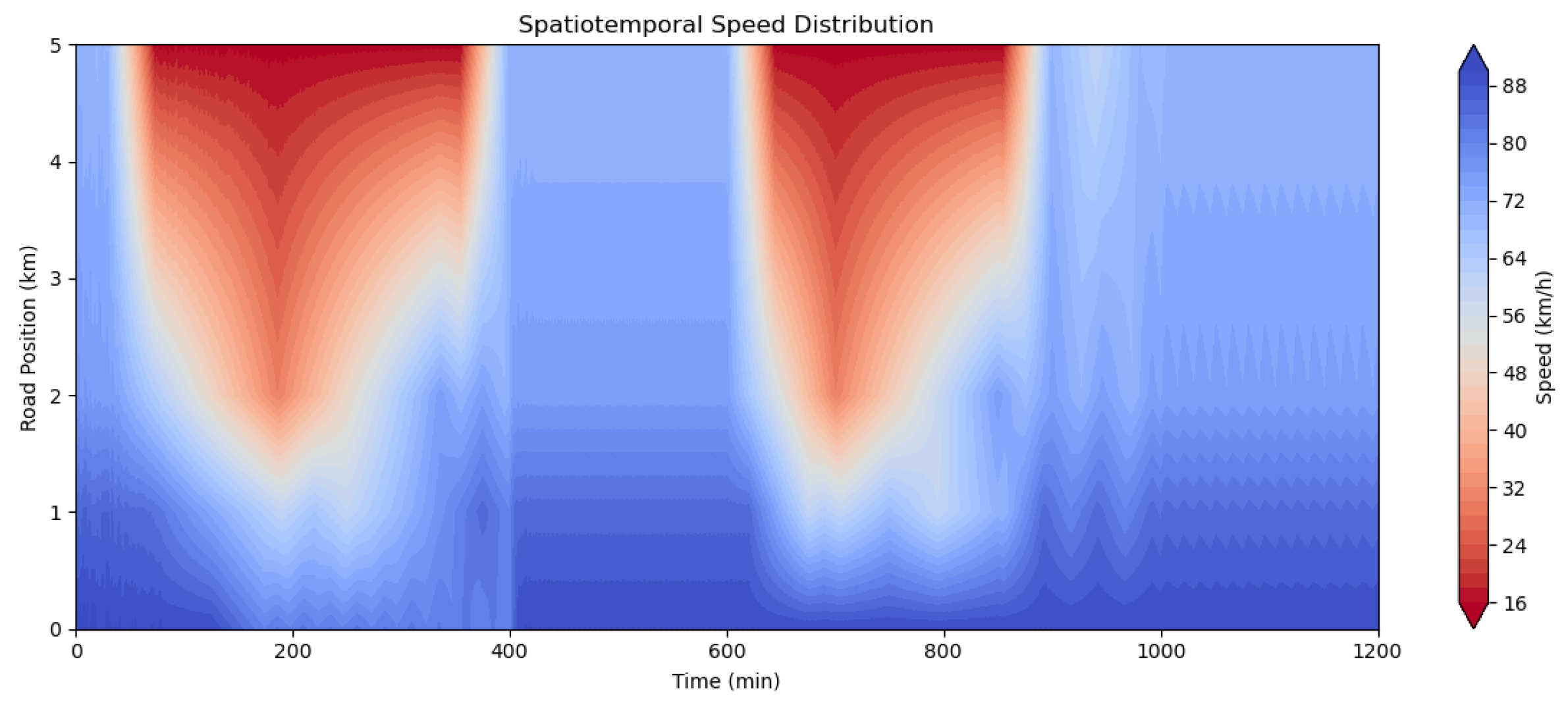
Figure 1. Speed Spatiotemporal Diagram of Highway Observation Section (color from blue to red indicates speed from high to low).
Sustainability 17 08327 g001
Figure 2. Measured Speed-Flow Relationship Scatter Plot at Observation Point.
Sustainability 17 08327 g002
Figure 3. Three-dimensional Speed-Density-Flow Relationship Diagram.
Sustainability 17 08327 g003
Figure 4. Kriging Surrogate Model Prediction Accuracy Verification.
Sustainability 17 08327 g004
Figure 5. Surrogate Model Prediction Confidence Interval Analysis.
Sustainability 17 08327 g005
Figure 6. Convergence Curve of Genetic Algorithm Evolution Process.
Sustainability 17 08327 g006
Figure 7. Efficiency-Safety Bi-objective Pareto Solution Set: Total Travel Time vs. Total Exposure Time Relationship.
Sustainability 17 08327 g007
Figure 8. Schematic Diagram of Optimized Emergency Lane Activation Strategy.
Sustainability 17 08327 g008
Figure 9. Comparison of Traditional Threshold Method and Optimization Method Activation Strategies.
Sustainability 17 08327 g009
Figure 10. Impact of Objective Weight on Optimization Results.
Sustainability 17 08327 g010
Table 1. Statistical Values of Traffic Parameters at Each Observation Point.
ParameterPoint 1Point 2Point 3Point 4
Average Density (veh/km)28.534.746.252.6
Average Speed (km/h)86.775.468.162.3
Average Flow (veh/h)2470261429502867
Flow Standard Deviation (veh/h)621736798842
Congestion Proportion (speed < 60 km/h)14.2%25.8%38.5%46.7%
Table 2. Kriging Surrogate Model Performance Metrics (5-fold Cross-validation).
Performance MetricTTT ModelTET Model
R20.9780.936
RMSE21.518.7
MAE18.614.7
Average Relative Error2.2%5.3%
Table 3. Comparison of Surrogate Model and Direct Simulation Methods.
MethodTotal Evals.Actual Sims.Comp. TimeBest TTTBest TET
Direct Simulation20002000∼3 h652192
Surrogate Model2100100∼10 min650198
Improvement Ratio-95%94.4%0.3%−3.1%
Table 4. Comparison of Simulation Effects of Different Emergency Lane Activation Strategies.
SchemeAverage SpeedAverage Travel TimeTotal Travel TimeTotal Dangerous Exposure TimeDangerous EventsThroughput
A: Non-activation35 km/h8.2 min950 veh·min0 s0348
B: Always-activated60 km/h5.4 min650 veh·min290 s57452
P: Optimized Scheme52 km/h6.2 min750 veh·min210 s40438
Simplified Threshold Scheme51 km/h6.4 min780 veh·min216 s42435
Table 5. Comparison of Traditional Threshold Method and Optimization Method Effects.
Performance IndicatorNon-ActivationTraditional Threshold MethodOptimization MethodRelative Improvement of Optimization Method
Total Travel Time9507707502.6%
Total Exposure Time025621018.0%
Dangerous Events Count0504020.0%
Total Emergency Lane Activation Time0302033.3%
Table 6. Performance of Compromise Scheme Under Different Demand Levels.
Performance IndicatorLow Load (0.9 Times)Baseline LoadHigh Load (1.1 Times)
Total Travel Time680750940
Total Exposure Time180210315
Average Travel Time5.86.27.6
Emergency Lane Activation Time102035
Disclaimer/Publisher’s Note: The statements, opinions and data contained in all publications are solely those of the individual author(s) and contributor(s) and not of MDPI and/or the editor(s). MDPI and/or the editor(s) disclaim responsibility for any injury to people or property resulting from any ideas, methods, instructions or products referred to in the content.