Development Dynamics and Influencing Factors of China’s Agricultural Green Ecological Efficiency Based on an Evaluation Model Incorporating Ecosystem Service Value and Carbon Emissions

Abstract

Sustainable agricultural development requires ensuring food security while preserving essential ecological conditions. This study incorporated ecosystem service value and carbon emissions as the positive and negative ecological outputs of agriculture, respectively, to account for the AGEE of 31 Chinese provinces from 2012 to 2021 and to analyse its spatiotemporal characteristics. The Malmquist Index was employed to calculate the green total factor productivity (GTP) as a quantitative indicator of AGEE dynamics, providing further insights into the sources and equilibrium of AGEE growth, as well as provincial-level improvement paths. Furthermore, the Spatial Durbin Model was applied to systematically analyse the influencing factors and their associated spatial spillover effects. The results show the following: (1) AGEE demonstrated steady improvement, with a mean value of 0.576, and was spatially concentrated along a northeast–southwest axis, exhibiting regional disparities and polarisation. (2) GTP consistently exceeded 1, indicating overall AGEE growth, primarily driven by technological scale expansion. Regional imbalances in AGEE growth had emerged, with heterogeneous causes across economic regions. Three identified AGEE improvement paths—technological catch-up, green innovation, and technological progress—varied by province, with green innovation being the most common priority. (3) AGEE exhibited spatial autocorrelation, with rural income, adequate irrigation, and cropping structure promoting AGEE. Effective irrigation also exhibited a positive spatial spillover effect, whereas industrial structure hindered AGEE. These findings provide valuable insights for advancing green agricultural practices and sustainable regional development.

1. Introduction

Agriculture, as a foundational industry of China’s socio-economic system, has consistently been integrated into the core of the national strategic agenda and has achieved remarkable progress [1,2,3,4]. Amid the intensifying global food crisis, China sustained two decades of grain production growth, reaching a new record of 707 million tons in 2024. With a per capita grain availability of 501.8 kg, which is considerably higher than the 400-kg threshold commonly used to assess food security, China maintains a strong position in ensuring national food supply [5]. Nevertheless, frequent international conflicts have severely disrupted global food supply chains, while accelerated urbanisation, combined with demographic ageing, has fuelled a persistent and increasingly inflexible rise in food demand [6,7]. Under such circumstances, ensuring food security remains the primary task in China’s agricultural development in the foreseeable future [8]. Meanwhile, China’s agricultural development is increasingly constrained by resource and environmental limitations. The country must support nearly 18% of the global population despite its severely limited land and water endowments—having less than 40% of the global average per capita arable land and only one-quarter of the per capita water resources [9,10,11]. Over the past few decades, the intensive agricultural model, characterised by excessive resource inputs and environmental burdens, has exacerbated the depletion of arable land and water supplies, while significantly increasing greenhouse gas emissions and intensifying diffuse agricultural pollution [12]. Against this backdrop, China’s agricultural sector must adopt sustainable development principles, aiming to satisfy rising food demands while safeguarding the ecological foundations critical to long-term agricultural viability [13,14].

Agricultural green ecological efficiency (AGEE) has emerged as a key metric for evaluating regional progress toward sustainable agriculture, drawing increasing attention from both policymakers and scholars [15,16]. AGEE is generally defined as the capacity to maximise desirable agricultural outputs while minimising resource consumption and ecological degradation, reflecting the synergy between economic development and ecological protection in agricultural production [17]. Among the various environmental issues arising from agricultural production, agricultural carbon emissions hold a particularly high strategic priority. This is not only due to agriculture’s substantial contribution to global carbon emissions (accounting for 17%) [18,19], but also stems from the explicit emission reduction requirements imposed by the Chinese government’s “dual carbon” goals [20,21]. Meanwhile, agricultural output encompasses not only the direct economic value of farm products but also the often-overlooked ecosystem services value (ESV) [22,23]. Agricultural ecosystem services include gas regulation [24], pollination facilitation [25], biodiversity increase [26], social relationship enhancement [27], and the provision of aesthetic landscapes—representing diverse natural benefits humans derive from agroecosystems. However, prior AGEE assessments have largely emphasised carbon emissions and economic value while giving limited consideration to ESV, which may bias efficiency estimates away from the actual state of sustainable agricultural development [28,29,30]. Accordingly, to capture both the positive and negative ecological externalities embedded in China’s agricultural production, we incorporate carbon emissions and ESV simultaneously into the AGEE accounting framework. The Malmquist Index (MI) provides a powerful tool for quantifying the dynamic changes in AGEE and disentangling the specific contributions of technological factors [31]. Moreover, given China’s vast territory and significant disparities in natural endowments and development conditions across regions, progress in AGEE has been uneven. At the national level, narrowing interregional gaps in AGEE advancement and promoting equity are essential safeguards for sustainable green agricultural development; at the provincial level, place-based strategies are needed to design differentiated improvement paths aligned with each region’s AGEE profile. However, in the agricultural sector, few studies have integrated the MI with regional heterogeneity to assess the convergence trends of AGEE growth, analyze the mechanisms behind such convergence, or identify province-specific improvement paths. This gap is particularly consequential for policy design: understanding whether AGEE is rising and the sources of that growth can anchor policies that promote green, sustainable agriculture, while analyzing regional convergence and divergent development paths across provinces can improve resource allocation and advance balanced regional development.

Beyond intrinsic technical factors, AGEE is also shaped by exogenous factors. Existing studies have identified the roles of socio-economic variables, such as population ageing, per capita GDP, and urbanisation [32,33,34]. However, they often overlook the spatial effects arising from geographical linkages. Due to geographical proximity, similarities in resource endowments, and policy imitation, AGEE may exhibit spatial autocorrelation. Furthermore, with the increasing frequency of cross-regional flows of production factors and technology spillovers, it is imperative to introduce a spatial dimension when examining factors influencing AGEE. Based on the above analysis, we propose the following research questions: Within a framework that simultaneously accounts for carbon emissions and ESV, what spatiotemporal patterns does AGEE exhibit? Has AGEE achieved sustained growth, and which technological components drive that growth? Given pronounced regional disparities, does AGEE growth display convergence—and through what mechanisms? How should provinces select suitable improvement paths? Moreover, as regional interactions intensify, do the factors influencing AGEE display spatial interdependence?

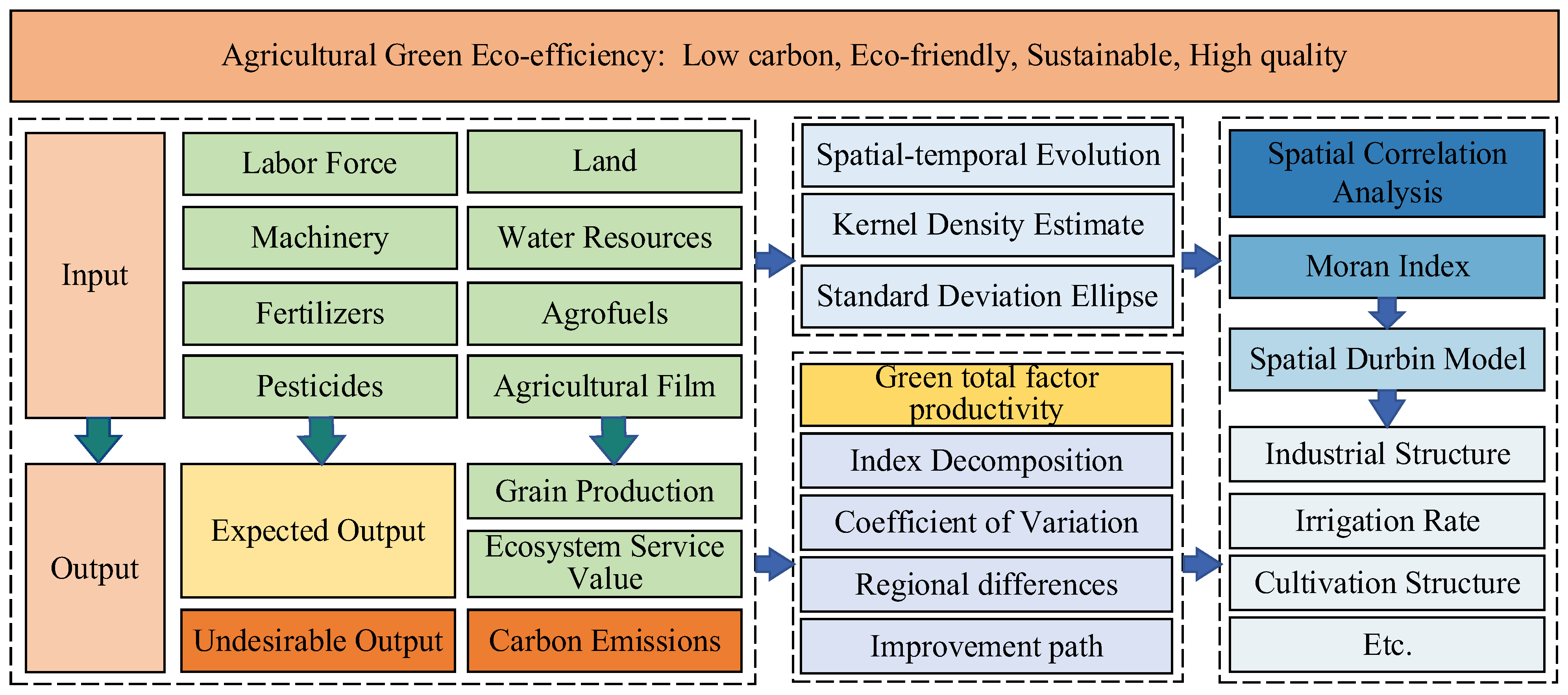
In response to these questions, this study first integrated carbon emissions and ESV to account for AGEE in China, employing kernel density estimation and the standard-deviation ellipse (SDE) to identify its spatiotemporal evolution. Secondly, the Malmquist index was used to compute the green total factor productivity (GTP) as a quantitative indicator of AGEE dynamics, examining the specific contributions of three technological components: MATC, BTC, and EC. Subsequently, the coefficient of variation and variance decomposition were applied to reveal the convergence trends and mechanisms underlying the AGEE dynamics. Finally, the spatial Durbin model was utilised to analyse the AGEE’s influencing factors and their associated spatial spillover effects.

This study makes three contributions. First, by integrating both the positive and negative ecological externalities of agriculture, we develop an AGEE accounting framework that combines ESV and carbon emissions, providing a more comprehensive—and policy-relevant—basis for subsequent efficiency assessments. Second, we use the Malmquist index and its decomposition to elucidate the drivers and regional heterogeneity of AGEE growth, thereby identifying province-level, differentiated improvement paths for tailored policy design. Third, we introduce spatial econometric methods to examine the spatial spillovers of factors influencing AGEE, advancing our understanding of interregional linkages and coordinated development mechanisms, and offering a theoretical basis for cross-regional agri-environmental governance. The research framework is shown in Figure 1.

2. Literature Review

The concept of eco-efficiency first emerged in the 1990s, aiming to maximise the fulfilment of human needs while minimising resource consumption and environmental pollution [35,36]. With the advancement of the global sustainable development agenda, this concept has been widely applied to urban systems [37,38], the energy sector [39,40], manufacturing [41], and many other fields and has gradually been extended to agriculture. Agricultural Green Ecological Efficiency (AGEE) refers to achieving the greatest possible agricultural output with limited resource inputs while minimising environmental pollution [30]. Internationally, similar concepts include Sustainable Intensification in Agriculture [42], green agricultural productivity [43], agricultural carbon efficiency [44], and Agricultural Green Development Efficiency [45], among others. Current academic research primarily focuses on three aspects: the accounting of AGEE, its multi-perspective assessment, and the analysis of influencing factors.

2.1. AGEE Accounting Model

Methods for accounting agricultural eco-efficiency include the life-cycle approach [46], ecological footprint analysis [47], ratio methods [48], and stochastic frontier analysis [49]. Compared to these methods, nonparametric methods, such as data envelopment analysis (DEA), offer clear advantages in handling multi-input, multi-output systems without prespecifying a production function—an especially relevant feature for agricultural systems, characterised by diverse resource structures and output types [30]. However, traditional DEA models fail to incorporate undesirable outputs, thus inaccurately reflecting efficiency losses due to environmental pollution and leading to biased eco-efficiency accounting. To address this issue, Tone (2002) [50] proposed the super-efficiency slack-based measure (Super-SBM) model that explicitly accommodates undesirable outputs. This model captures both desirable and undesirable outputs and allows further discrimination among efficient decision-making units, thereby improving precision and separability. This approach has been widely applied to agricultural eco-efficiency studies [30,44]. Following the mainstream, this study adopts the Super-SBM to construct a composite AGEE accounting measure.

Regarding indicator selection, based on insights into agricultural system inputs and outputs, existing studies have reached a relatively high consensus on input indicators, typically including labour, land, machinery, irrigation water, and pesticide use [51,52,53]. For output indicators, studies have emphasised economic outcomes and environmental impacts. For example, Chi et al. (2022) [54] and Ge et al. (2023) [45] selected agricultural value added as a desirable output and carbon emissions as an undesirable output, respectively. Yu and Wei (2025) [55] further incorporated crop yield and diffuse agricultural pollution to evaluate cultivated land-use efficiency. However, these studies often overlook the ecosystem service value (ESV)—the direct benefits agroecosystems provide to humans. Although balancing economic and ecological value has become a global consensus for sustainable agriculture [17,56], incorporating ESV into AGEE accounting remains limited [28,29,30]. In practice, continued exploitation of agricultural resources can constrain the realisation of ESV [57]; ignoring ESV as part of desirable outputs may therefore bias AGEE accounting away from the actual state of sustainable development. Accordingly, within the Super-SBM framework, we develop an AGEE indicator system that simultaneously integrates ESV and carbon emissions. Compared to prior work, this accounting framework better captures agriculture’s multifunctionality, avoids one-sided underestimation in regions of high ecological value, and provides a more rigorous and equitable basis for subsequent efficiency assessments.

2.2. Multi-Perspective Assessment of AGEE

Assessment based on efficiency accounting results can be broadly categorised into two perspectives: “growth” in the temporal dimension and “equity” in the spatial dimension. Temporally, numerous studies document the evolution of AGEE across countries and regions. For example, Wang et al. (2024) [58] measured the agricultural energy efficiency of 144 countries across five continents from 2011 to 2021, finding a significant increase in all regions except Oceania. Liu et al. (2020) [33] reported a 76% increase in provincial agricultural eco-efficiency in China over the past four decades. However, such time-trend descriptions based on cross-sectional snapshots yield only limited qualitative insights. The Malmquist index (MI) provides a stronger tool by offering a quantitative measure of efficiency growth and decomposing it into contributions from technical change (TC) and technical efficiency (TE). In agriculture, the MI approach has seen increasing use. For example, Yang et al. (2022) [31] found that the growth rate of agricultural eco-efficiency across Chinese provinces from 2001 to 2018 was relatively low, with TC being the key driver; Chivu et al. (2020) [59] likewise found productivity gains in U.S. agricultural cooperatives to be driven by TC rather than EC. A standard limitation in these studies is the default assumption of Hicks-neutral TC. In reality, technological progress in most regions and sectors is biased [60]—whether it involves input-saving on the production side or is aimed at reducing undesirable outputs, such as CO₂, on the outcome side—reflecting a shift toward greener technologies [61]. Disentangling the biased component within TC is therefore crucial for accurately identifying the underlying drivers of AGEE growth. In this vein, Liu et al. (2022) [61] decomposed green TFP into technical efficiency (EC), biased technical change (BTC), and magnitude of technological change (MATC), and examined how environmental regulation affects manufacturing productivity and its components. Related applications to agriculture, however, remain scarce.

Spatially, pronounced regional imbalance in AGEE is widespread, particularly in developing countries and regions with intensive agriculture, owing to heterogeneity in development bases and natural endowments. Wang et al. (2024) [58] emphasised the large and widening regional gaps in global agricultural energy efficiency. At the farm level in Africa, Gollin and Udry (2020) [62] documented substantial productivity dispersion. Using the Dagum Gini decomposition, Jin et al. (2024) [44] showed that within-region differences are the primary source of overall disparity in agricultural carbon efficiency across China’s three major grain-production zones. While these studies underscore the importance of spatial heterogeneity, most focus on static indicators. In fact, regional gaps in AGEE reflect the cumulative outcomes of divergent growth dynamics; examining convergence in AGEE growth can yield more fundamental insights for balanced regional development. Probing the mechanisms behind divergence is likewise essential for policies that enhance equity. The limited existing work that employs econometric models or GeoDetector highlights the role of resource inputs in shaping spatial disparities [30,44] but largely neglects technological factors as fundamental sources of these differences.

2.3. Factors Influencing AGEE

In recent years, a growing body of research has focused on various socio-economic factors affecting AGEE. Li et al. (2022) [63] employed a PVAR model to analyse the long-run equilibrium among population ageing, renewable resource consumption, and agricultural green productivity, while Zhao et al. (2023) [34] detailed the channels through which urbanisation—as a core driver—affects agricultural eco-efficiency. However, due to geographical proximity, similarities in resource endowments, and policy imitation behaviour, AGEE is likely to exhibit spatial autocorrelation. Moreover, the frequent interregional flow of production factors and technology spillovers between neighboring provinces may lead to cross-regional effects of various influencing factors. It is therefore necessary to incorporate geographic variables to broaden analyses of AGEE’s influencing factors.

Taken together, the existing literature still shows three salient gaps: (1) Indicator selection for AGEE accounting. Most studies focus solely on ecological negative externalities, treating carbon emissions and other pollutants as undesirable outputs, while overlooking the substantial benefits provided by ecosystems. This omission can bias AGEE accounting away from the actual state of sustainable agricultural development. (2) Limited understanding of AGEE dynamics. The conventional assumption of Hicks-neutral technological progress is not only unrealistic but also hinders the identification of the fundamental drivers behind AGEE growth. Furthermore, assessments of “growth” and “equity” are often conducted in isolation, failing to provide practical insights for achieving regionally coordinated AGEE development. (3) There is a lack of in-depth investigation into the spillover mechanisms of various exogenous factors affecting AGEE. To address these gaps, this study constructs a more comprehensive analytical framework for AGEE. It refines the sources of AGEE dynamics into MATC, BTC, and EC, examines both the regional equity of AGEE growth and its underlying causes, and thoroughly investigates the comprehensive impact of exogenous factors—including their spatial spillover effects. This study aims to provide a more comprehensive and detailed understanding of AGEE in China, thereby supporting the identification of effective strategies to promote the achievement of sustainable agricultural development goals.

3. Methods and Materials

3.1. Research Methods

3.1.1. Accounting Methods of Agricultural Ecosystem Service Value and Carbon Emission

(1)

Assessment of agricultural ecosystem service value

Agriculture fosters synergistic social, economic, and cultural development while also enhancing human health. The ecosystem service value measurement method was first proposed by Costanza et al. (1997) [56]. Based on this approach, Xie et al. (2015) [64] proposed and updated a widely used evaluation framework for China’s terrestrial ecosystems, assigning ecological service values to each unit of land area. In this study, we calculated the agricultural ecosystem service values of Chinese provinces by combining the cultivated land valuation coefficients revised by Xie et al. (2015) [64] with regional adjustment factors that reflect differences in farmland biomass productivity (

Table 1. Biomass factors of the cultivated land ecosystem in China.

Province	Biomass Factor	Province	Biomass Factor	Province	Biomass Factor
Hunan	1.95	Chongqing	1.21	Ningxia	0.64
Zhejiang	1.76	Anhui	1.17	Yunnan	0.64
Jiangsu	1.74	Beijing	1.04	Guizhou	0.63
Fujian	1.56	Hebei	1.02	Xinjiang	0.58
Jiangxi	1.51	Jilin	0.96	Shaanxi	0.51
Shanghai	1.44	Guangxi	0.98	Shanxi	0.46
Guangdong	1.40	Liaoning	0.90	Inner Mongolia	0.44
Henan	1.39	Tianjin	0.85	Gansu	0.42
Shandong	1.38	Xizang	0.75	Qinghai	0.04
Sichuan	1.35	Hainan	0.72	China	1.00
Hubei	1.27	Heilongjiang	0.66

). The agricultural ecosystem service value is computed using the following formula:

$$ES{V}_{it}=A_{it}\times C{F}_i\times {\displaystyle \sum _{n=1}^{7}E{C}_n}\times ({\displaystyle \raisebox{1ex}{$1$}\!\left/ \!\raisebox{-1ex}{$7$}\right.})\times {\displaystyle \sum _{k=1}^4\frac{p_{ikt}\times q_{ikt}\times m_{ikt}}{A_{it}}}$$

(1)

where ${\mathit{ESV}}_{\mathit{it}}$is the agriculture ecosystem service value, $A_{\mathit{it}}$ denotes the total planting area (hm²) of food crops in province $i$ for year $t$, and ${CF}_i$ is the correction factor for each province based on biomass factors [65]. ${EC}_n$ irepresents the ecological service equivalent value factors for each function (gas regulation = 0.50, climate regulation = 0.89, hydrological regulation = 0.60, waste treatment = 1.64, soil conservation = 1.46, biodiversity maintenance = 0.71, aesthetic landscape provision = 0.01). $k$ refers to the type of food crop, with rice, maize, wheat, and soybeans selected as the four primary food crops for this study. $p_{\mathit{ikt}}$, $q_{\mathit{ikt}}$, and $m_{\mathit{ikt}}$ represent the average price (CNY/ton), unit area yield (ton/ hm²), and planting area (hm²) of crop $k$ in province $i$ for year $t$, respectively.

(2)

Agricultural carbon emissions Measurement

This study employed the IPCC emission factor method to estimate agricultural carbon emissions, owing to its systematics and strong comparability, which make it suitable for regional-scale carbon emission estimation [66]. It calculates total emissions by summing the products of activity data and their corresponding emission coefficients, and has been widely applied in global and regional agricultural carbon assessments [67,68,69]. Based on the IPCC framework and China’s agricultural practices, we construct the following formula for agricultural carbon emissions:

$$E_t=GM+TN+SO+PQ+FR+AU$$

(2)

where $E_t$is carbon emissions from agriculture, $G,T,S,P,F,A$ correspond to the quantities of fertiliser applied, pesticide usage, the area under cultivation, the total horsepower of agricultural machinery, irrigated farmland, and the extent of plastic film application in agriculture, respectively, and $M,N,O,Q,R,U$ are conversion factors. To ensure consistency and comparability, we selected carbon emission sources and their conversion factors that are consistent with previous studies [68,70], specific values and references are shown in

Table 2. Carbon emission sources and conversion factors.

Carbon Emission Source	Conversion Factor	References
Fertiliser	0.8956 kg C/kg	Huang et al. [68]; Han et al. [66]; Jing et al. [70]
Pesticide	4.9341 kg C/kg	Huang et al. [68]; Han et al. [66]; Jing et al. [70]
Cultivation	16.47 kg/hm2	Feng et al. [71]; Jing et al. [70]
Agriculture machinery	0.18 kg/kW	Feng et al. [71]; Jing et al. [70]
Irrigation	266.48 kg/hm2	Huang et al. [68]; Han et al. [66]; Jing et al. [70]
Agricultural film	5.18 kg/hm2	Huang et al. [68]; Han et al. [66]; Jing et al. [70]

.

3.1.2. Super-Efficient SBM-DEA Modelling

The traditional DEA method for assessing agricultural efficiency primarily focuses on economic performance, overlooking the repercussions of non-desired by-products, and thereby fails to accurately reflect the realities of the agricultural production process. This oversight also needs to pay more attention to input and output slackness, distorting the actual efficiency of agricultural resource utilisation. To address these issues, the slack-based measure (SBM) model, known for being non-radial and non-oriented, was introduced by Tone (2001) [72]. This approach incorporates input and output slacks directly into the objective function, improving the precision of empirical evaluations. Building on this, the super-efficiency SBM model, designed to distinguish between entities with efficiency scores 1, was proposed by Tone (2002) [50] to refine agricultural efficiency evaluation. The specific calculation formula is as follows:

$$Min\rho ={\displaystyle \frac{1+\frac{1}{m}{\displaystyle \sum _{i=1}^m\left(S_i^x/{x^t}_{ik}\right)}}{1-\frac{1}{r_1+r_2}\left({\displaystyle \sum _{s=1}^{r_1}{S}_s^y/y_{sk}^t+{\displaystyle \sum _{q=1}^{r_2}{S}_q^z/z_{qk}^t}}\right)}}$$

(3)

$$s.t.\left\{\begin{array}{l}{x}_{ik}\ge {\displaystyle \sum _{j=1,\ne k}^n{x}_{ij}{\lambda }_j-}{S}_i^x\\ y_{sk}\le {\displaystyle \sum _{j=1,\ne k}^n{y}_{sj}{\lambda }_j+}{S}_s^y\\ z_{qk}\ge {\displaystyle \sum _{j=1,\ne k}^n{z}_{qj}{\lambda }_j-}{S}_q^z\\ {\lambda }_j\ge 0,S_i^x\ge 0,S_s^y\ge 0,S_q^z\ge 0,\\ i=1,2,\dots ,m;s=1,2,\dots ,r_1;q=1,2,\dots ,r_2;j=1,2,3,\dots ,n\end{array}\right.$$

(4)

where $\rho$ is the AGEE in each province, n indicates the quantity of DMUs. m, $r_1$, and $r_2$ refer to the number of input, desired and undesired output variables, respectively. $x_{ik}$, $y_{sk}$, and $z_{qk}$ are the inputs, desirable outputs, and undesirable outputs of the $k\mathrm{th}$ DMU. $S_i^x$, $S_s^y$, and $S_q^z$ represent the slack of inputs, desirable outputs, and undesirable outputs. ${\lambda }_j$ is the weighting coefficient.

3.1.3. Malmquist Index Model

Based on the distance functions derived from the super-SBM model, the Malmquist productivity index was constructed. Following the framework of Färe et al. (2006) [73] green total factor productivity (GTP) is decomposed into efficiency change (EC) and technical change (TC), with TC further partitioned into the magnitude of technological change (MATC) and biased technological change (BTC).

$$GT{P}_k^{t,t+1}={\left[{\displaystyle \frac{{\rho }_k^t\left(x^{t+1},y^{t+1},z^{t+1}\right)}{{\rho }_k^t\left(x^t,y^t,z^t\right)}}\times {\displaystyle \frac{{\rho }_k^{t+1}\left(x^{t+1},y^{t+1},z^{t+1}\right)}{{\rho }_k^{t+1}\left(x^t,y^t,z^t\right)}}\right]}^{{\displaystyle \frac{1}{2}}}$$

(5)

where ${\rho }_k^t(x^t,y^t,z^t)$and ${\rho }_k^{t+1}(x^t,y^t,z^t)$ denote the efficiency of the $k\mathrm{th}$ DMU at period $t$ and $t+1$, respectively. ${\mathit{GTP}}_k^{t,t+1}$ represents the change rate of AGEE for $k\mathrm{th}$ DMU from period $t$ to $t+1$. When ${\mathit{GTP}}_k^{t,t+1}$ > 1, it means that the DMU $k$’s AGEE performance has improved; otherwise, a decline is indicated. Further decomposition of the above equation is obtained:

$$\begin{array}{l}GT{P}_k^{t,t+1}=T{C}_k^{t,t+1}\times E{C}_k^{t,t+1}\\ =\left[{\displaystyle \frac{{\rho }_k^t\left(x^t,y^t,z^t\right)}{{\rho }_k^{t+1}\left(x^t,y^t,z^t\right)}}\times {\displaystyle \frac{{\rho }_k^t\left(x^{t+1},y^{t+1},z^{t+1}\right)}{{\rho }_k^{t+1}\left(x^{t+1},y^{t+1},z^{t+1}\right)}}\right]{\times }^{{\displaystyle \frac{1}{2}}}\times {\displaystyle \frac{{\rho }_k^{t+1}\left(x^{t+1},y^{t+1},z^{t+1}\right)}{{\rho }_k^t\left(x^t,y^t,z^t\right)}}\end{array}$$

(6)

where ${\mathit{TC}}_k^{t,t+1}$ denotes the technological change, namely the evolution of the production frontier, in the $k\mathrm{th}$ DMU during the interval from t to t+1, ${\mathit{EC}}_k^{t,t+1}$ denotes the relative efficiency change, which evaluates how the $k\mathrm{th}$ DMU narrows the gap relative to the prevailing environmental production technologies during the same time frame. When EC > 1, it reflects an improvement in efficiency and, vice versa, a decline.

The index $\mathit{TC}$ is further decomposed into the magnitude of technological change $\left(\mathit{MATC}\right)$and biased technological change $\left(\mathit{BTC}\right)$. The specific formula is as follows:

$$\begin{array}{l}T{C}_k^{t,t+1}={\left[{\displaystyle \frac{{\rho }_k^t\left(x^t,y^t,z^t\right)}{{\rho }_k^{t+1}\left(x^t,y^t,z^t\right)}}\times {\displaystyle \frac{{\rho }_k^t\left(x^{t+1},y^{t+1},z^{t+1}\right)}{{\rho }_k^{t+1}\left(x^{t+1},y^{t+1},z^{t+1}\right)}}\right]}^{{\displaystyle \frac{1}{2}}}\\ ={\displaystyle \frac{{\rho }_k^t\left(x^{t+1},y^{t+1},z^{t+1}\right)}{{\rho }_k^{t+1}\left(x^{t+1},y^{t+1},z^{t+1}\right)}}\times {\left[{\displaystyle \frac{{\rho }_k^t\left(x^t,y^t,z^t\right)}{{\rho }_k^{t+1}\left(x^t,y^t,z^t\right)}}\times {\displaystyle \frac{{\rho }_k^{t+1}\left(x^{t+1},y^{t+1},z^{t+1}\right)}{{\rho }_k^t\left(x^{t+1},y^{t+1},z^{t+1}\right)}}\right]}^{{\displaystyle \frac{1}{2}}}\\ =MAT{C}_k^{t,t+1}\times BT{C}_k^{t,t+1}\end{array}$$

(7)

MATC represents the magnitude of technological progress, capturing the overall outward shift in the group frontier. In our study, $\mathit{MATC}>1$ indicates a general-purpose technological breakthrough, where the efficiency of all input factors improves proportionally. In contrast, $\mathit{BTC}$ reflects the directional shift in the group frontier, characterising technological progress that favours specific resource conservation or desirable output augmentation. In our study, $\mathit{BTC}>1$ implies that technological progress is characterised by energy saving and emission reduction, highlighting its green orientation.

3.1.4. Exploratory Spatial Data Analysis (ESDA)

(1)

Spatial Autocorrelation Model

Global spatial autocorrelation, assessed via Moran’s I, is employed to evaluate spatial associations of AGEE across the entire study area. Its formula is

$$Moran’s I={\displaystyle \frac{n}{{\displaystyle \sum _{i=1}^n{\displaystyle \sum _{j=1}^n{w}_{ij}}}}}\times {\displaystyle \frac{{\displaystyle \sum _{i=1}^n{\displaystyle \sum _{j=1}^n{w}_{ij}\left({\theta }_i-\overline{\theta }\right)\left({\theta }_j-\overline{\theta }\right)}}}{{\displaystyle \sum _{i=1}^n{\left({\theta }_i-\overline{\theta }\right)}^2}}}$$

(8)

where $n$ denotes the total number of provinces under study; ${\theta }_i$ and ${\theta }_j$ represent AGEE of location $i$ and $j$ ($i\ne j$);$\overline{\theta }$ is their mean, and $W$ indicates the spatial weight matrix.

Given the spatial uniformity assumption of global autocorrelation, it fails to capture localised clustering patterns. Therefore, to explore the spatial heterogeneity and aggregation of AGEE at the local scale, local spatial autocorrelation analysis is adopted [74], and its calculation formula is

$$Moran’s I_i={\displaystyle \frac{\left({\theta }_i-\overline{\theta }\right)}{{\displaystyle \sum _{i=1}^n{\left({\theta }_i-\overline{\theta }\right)}^2}}}{\displaystyle \sum _{j\ne 1}^n{w}_{ij}\left({\theta }_j-\overline{\theta }\right)}$$

(9)

where $I_i$ is the local Moran index for location $i$, $I_i$ is positive (negative), indicating that similar (dissimilar) AGEE regions are near each other, and a more considerable absolute value indicates a higher degree of proximity.

(2)

Spatial Durbin Model

To explore the influence of multiple factors on AGEE and their corresponding spatial spillover effects, this study applies the spatial Durbin model as an analytical framework. The calculation formula is as follows:

$$Ln({\theta }_{it})=\rho {\displaystyle {\sum }_{j=1}^n{w}_{ij}}({\theta }_{jt})+\beta X+{\displaystyle {\sum }_{j=1}^n{w}_{ij}{x}_{ijt}}\phi +{\mu }_i+{\delta }_t+{\epsilon }_{it}$$

(10)

where ${\theta }_{\mathit{it}}$ represents the AGEE of the $i\mathrm{th}$ province in $t$ year; $W$ denotes the spatial weight matrix. $\beta$ consists of parameters estimated for independent variables that influence AGEE; $\rho$ captures the spatial influence exerted by neighbouring provinces’ AGEE on local values; $\phi$ represents the spatial regression coefficient for the independent variables. ${\mu }_i$ and ${\delta }_t$ denote the spatial and temporal effects, respectively; and ${\epsilon }_{it}$ is the random error term. Based on prior research [21,34,75], this study incorporated a set of representative socio-economic and environmental variables as AGEE influencing factors, as detailed in

Table 3. Influencing Factors on AGEE.

Influencing Factors	Indicator Definition	Unit
Agriculture, forestry and water services ratio	The proportion of the local government budget allocated to agriculture, forestry, and water sectors	%
Aging rate	The proportion of the population aged 65 and over	%
Urbanization rate	The ratio of residents living in urban areas to the national population	%
Industrial structure	The degree of industrial structure upgrading 1 [75,76,77]	%
Disaster-affected rate	The ratio of crop area damaged by disasters to the total cultivated area	%
Rural per capita disposable income	Rural residents’ disposable income	Yuan
Effective irrigation rate	Effective irrigated area/sown area of food crops	%
Cultivation structure	Food crop planting area/crop planting area	%

¹ The corresponding measurement formula:$Industrial Structure Upgradin{g}_{it} ={\displaystyle \sum _{j=1}^3\frac{Y_{it,j}}{Y_{it}}}\times j$. Where $Y_{it,j}$ and $Y_{it}$ represent the output value of the$jth$industry and the total output value of province $i$ in year $t$, respectively.

.

3.2. Indicator and Data

3.2.1. Indicator Selection

Referring to relevant research results [52,53,78,79], considering the actual agricultural production process, we selected a total of eight indicators, including labor force, land, water resources, and chemical usage, such as pesticides and fertilizers, as agricultural production inputs. Total grain and agroecosystem service value were identified as the desired output of agricultural activities, while carbon emissions, as a concentrated manifestation of ecological negative externalities, were treated as undesirable output in agricultural production.

Table 4. AGEE input-output indicator system.

Indicator Category	Sub-Indicator	Indicator Description	Unit
Input indicators	Labor force	Number of agricultural workers	104 people
	Land	Area sown with food crops	103 hm2
	Machinery	Total installed capacity of agricultural machinery	104 kW
	Water resources	aggregate water utilization dedicated to farming activities	108 m3
	Fertilizer	Fertilizer application	104 t
	Agricultural Fuel	Agricultural diesel use	104 t
	Pesticides	Pesticide usage	104 t
	Agricultural film	Agricultural plastic film usage	t
Output indicators	Desired output	The total amount of grain	104 t
		Agroecosystem service value	108 Yuan
	Undesired output	Agricultural carbon emissions	104 t

presents the AGEE input–output indicator system.

3.2.2. Data Sources

AGEE reflects the comprehensive efficiency of agricultural production activities in protecting the ecological environment and enhancing economic efficiency. Adhering to the principles of data continuity, completeness, availability, and comparability, this study selected 31 provinces in China from 2012 to 2021 (due to missing data, the study scope excludes Hong Kong, Macao, and Taiwan) and categorizes the country into four broad economic zones—eastern, central, western, and northeastern—based on administrative geography and regional development characteristics. Relevant data—including the number of employees in the primary sector, grain-sown area, total agricultural machinery power, pesticide and fertiliser consumption, grain output, usage of agricultural film and fuel, and irrigated area—were compiled from official sources such as the China Rural Statistical Yearbook, the China Agricultural Yearbook, and the China Statistical Yearbook. Grain prices are from the National Summary of Cost and Benefit Information on Agricultural Products.

4. Research Results Analysis

4.1. Temporal and Spatial Analysis of AGEE

4.1.1. The Value of AGEE

Amidst the growing emphasis on environmental stewardship and sustainable growth, this study utilised MaxDEA Ultra 9 to assess AGEE in 31 Chinese provinces from 2012 to 2021. The findings, summarised in

Table 5. The value of AGEE by province in China.

Region	Province	2012	2013	2014	2015	2016	2017	2018	2019	2020	2021	Mean
Northeast	Liaoning	0.565	0.600	0.473	0.542	0.615	0.626	0.599	0.672	0.659	0.724	0.608
	Jilin	0.913	1.003	0.918	0.934	1.010	1.011	0.873	1.000	0.929	1.058	0.965
	Heilongjiang	1.002	1.001	1.004	1.006	0.946	0.935	0.920	1.008	1.012	1.061	0.989
Eastern	Beijing	0.391	0.364	0.281	0.310	0.299	0.272	0.262	0.252	0.275	0.317	0.302
	Tianjin	0.335	0.360	0.365	0.378	0.422	0.507	0.707	0.783	0.859	1.157	0.587
	Shanghai	0.691	0.677	0.629	0.665	0.660	0.687	1.013	1.004	1.000	1.038	0.807
	Hebei	0.413	0.425	0.421	0.427	0.485	0.503	0.518	0.547	0.608	0.631	0.498
	Shandong	0.452	0.459	0.475	0.492	0.534	0.553	0.563	0.580	0.613	0.647	0.537
	Jiangsu	0.635	0.635	0.681	0.725	0.700	0.775	0.855	0.925	0.960	1.003	0.789
	Zhejiang	0.312	0.282	0.289	0.280	0.290	0.297	0.337	0.340	0.367	0.376	0.317
	Fujian	0.257	0.253	0.249	0.243	0.243	0.250	0.259	0.261	0.274	0.281	0.257
	Guangdong	0.325	0.298	0.311	0.308	0.317	0.323	0.321	0.352	0.371	0.376	0.330
	Hainan	0.220	0.214	0.211	0.211	0.210	0.203	0.213	0.216	0.222	0.222	0.214
Central	Shanxi	0.486	0.499	0.508	0.477	0.551	0.580	0.603	0.598	0.643	0.646	0.559
	Henan	0.608	0.602	0.709	0.719	0.752	0.798	1.001	0.918	1.008	1.005	0.812
	Hubei	0.508	0.521	0.532	0.605	0.576	0.589	0.599	0.598	0.613	0.610	0.575
	Hunan	0.847	0.740	0.797	0.820	0.804	0.838	0.875	1.000	0.928	1.005	0.865
	Jiangxi	0.854	1.003	1.007	1.000	1.007	0.981	1.001	1.001	0.985	1.009	0.985
	Anhui	0.525	0.516	0.568	0.609	0.570	0.603	0.606	0.629	0.640	0.672	0.594
Western	Inner Mongolia	0.610	0.660	0.637	0.647	0.650	0.646	0.713	0.743	1.012	0.880	0.720
	Shaanxi	0.430	0.410	0.403	0.405	0.432	0.409	0.426	0.438	0.456	0.459	0.427
	Yunnan	0.363	0.368	0.367	0.361	0.362	0.367	0.505	0.513	0.504	0.530	0.424
	Guizhou	0.635	0.573	0.608	0.611	0.655	0.643	0.563	0.595	0.631	1.008	0.652
	Sichuan	0.639	0.646	0.634	0.636	0.656	0.658	0.670	0.680	0.704	0.715	0.664
	Chongqing	0.632	0.618	0.608	0.605	0.624	0.624	0.624	0.631	0.627	0.634	0.623
	Guangxi	0.333	0.330	0.325	0.316	0.317	0.314	0.320	0.313	0.326	0.334	0.323
	Gansu	0.345	0.340	0.337	0.331	0.343	0.351	0.377	0.389	0.410	0.432	0.365
	Qinghai	0.288	0.282	0.289	0.279	0.289	0.285	0.293	0.332	0.363	0.385	0.308
	Ningxia	0.439	0.433	0.489	0.472	0.493	0.528	1.001	0.839	1.010	0.822	0.653
	Tibet	0.484	0.437	0.443	0.432	0.435	0.469	0.507	0.546	0.595	1.068	0.542
	Xinjiang	0.465	1.002	0.556	1.003	0.379	0.368	0.387	0.401	0.425	0.566	0.555
	Mean	0.516	0.534	0.520	0.543	0.536	0.548	0.597	0.616	0.646	0.699	0.576

, revealed an overall upward yet fluctuating trend, with a mean AGEE of 0.576 (±0.22 SD), highlighting substantial variability across provinces and indicating significant potential for eco-efficiency enhancement despite the improvement. Regionally, Northeast China demonstrated the relatively high AGEE, with an average of 0.854 (±0.17 SD). Notably, this figure showed a year-on-year increase, indicating a solid trajectory towards greater eco-efficiency in agriculture. In contrast, the average AGEE values for China’s central and western regions were 0.732 (±0.20 SD) and 0.521 (±0.16 SD), respectively, while the eastern region registered the lowest level at 0.464 (±0.14 SD). The standard deviations indicate notable internal heterogeneity within each region, especially in the central and northeast areas, underscoring the need for differentiated policy interventions.

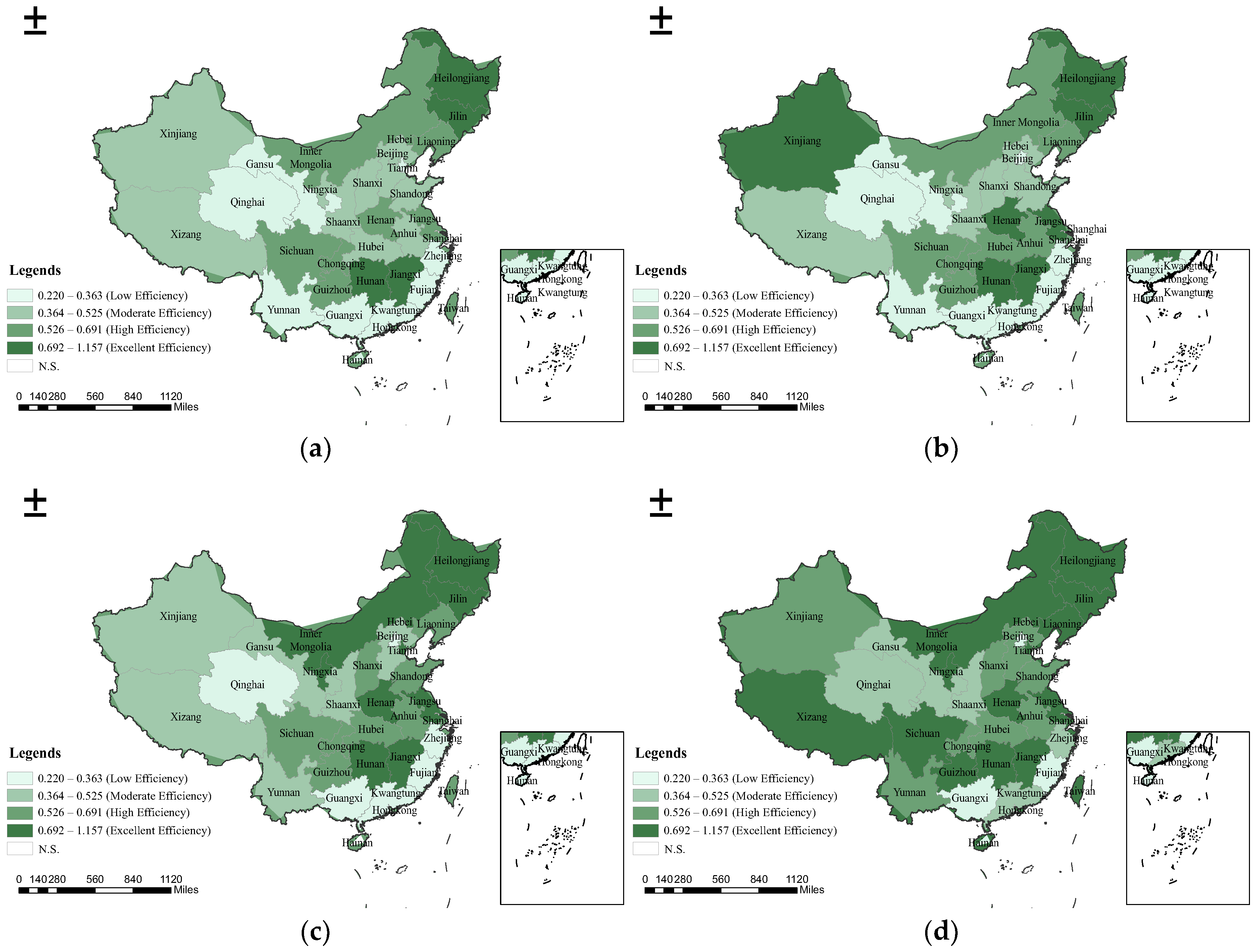
The spatial distribution of AGEE in China, mapped using ArcGIS 10.7, revealed a diverse and heterogeneous regional landscape (Figure 2). Provinces such as Jilin, Heilongjiang, Hunan, and Jiangxi consistently maintained high levels of AGEE, indicating their effective implementation of sustainable agricultural practices. In contrast, Guangxi, Fujian, and Hainan consistently demonstrated low levels of AGEE performance, underscoring the urgent need to formulate and accelerate green agricultural development strategies. Over time, the scope of regions with high AGEE levels steadily expanded. By 2021, the number of provinces classified as “low-efficiency” had declined to eight, with most provinces showing a clear transition to higher AGEE levels. Notably, Yunnan experienced the most significant upward shift, moving from the category of “low-efficiency” to “high efficiency,” which reflects the long-term effectiveness of its eco-agriculture policies. In contrast, the AGEE level in Xinjiang exhibited considerable fluctuations over time, highlighting the region’s dynamic and context-sensitive agroecological performance.

4.1.2. Kernel Density Distribution of AGEE

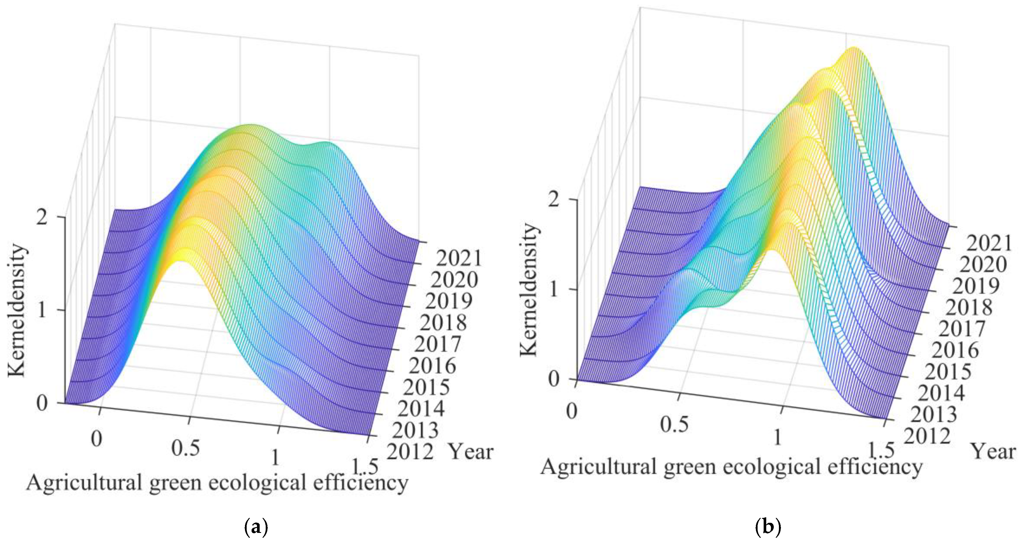
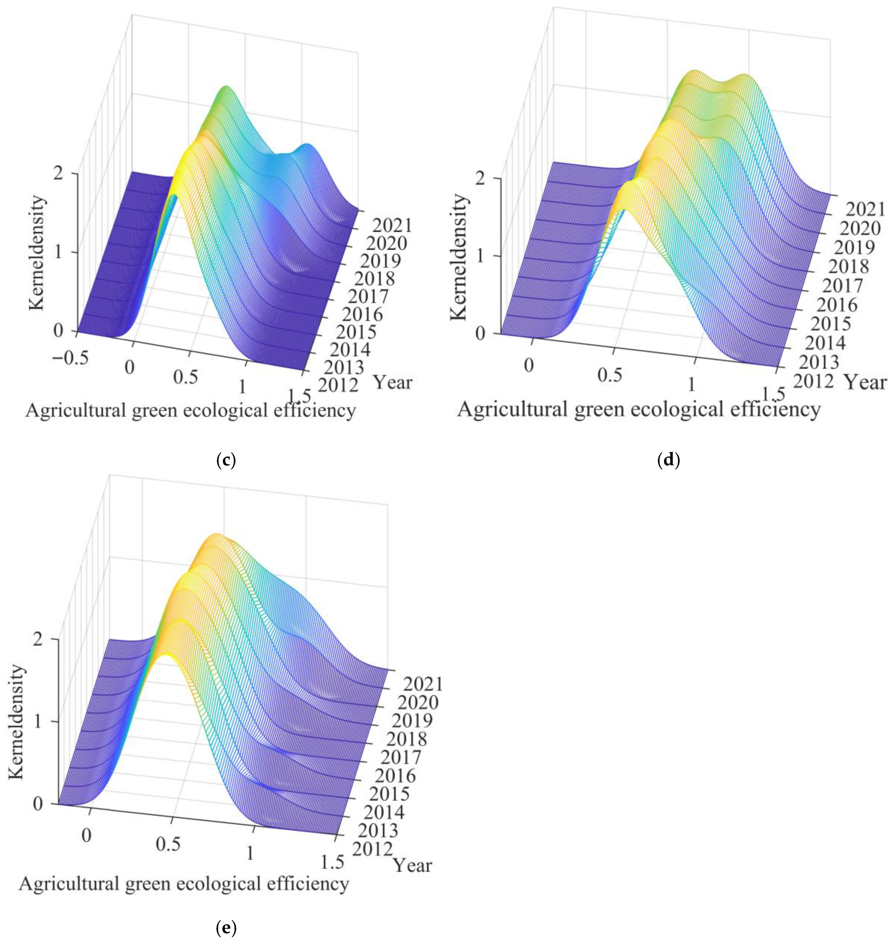
To investigate how AGEE values evolved, we applied kernel density estimation and plotted corresponding distribution curves for China as a whole and the four major regions: Northeast, East, Central, and West (Figure 3). Nationally, China’s AGEE kernel density distribution curve experienced a slight rightward shift during the study period, which indicates a general uptrend in overall efficiency. Concurrently, the central peak of the curve diminished, and the curve became flatter and wider, suggesting an expansion in regional disparities in AGEE across China. A prominent feature was a shift from a unimodal to a bimodal distribution, characterised by a widening divergence between the dominant and secondary modes—highlighting growing polarisation across provinces.

Regionally, Northeast China exhibited a notable shift in its kernel density curve—first leftward and then rightward—indicating that AGEE initially declined before rising again. A slightly rising and narrowing peak was observed, indicating convergence in regional AGEE levels. Moreover, the curve transitioned from a bimodal to a unimodal distribution, indicating a diminishing trend in regional polarisation. In the East, the peak location remained relatively stable, signalling a stable AGEE level throughout the study period. However, the curve evolved from a sharp, narrow profile to a flatter, wider one, reflecting growing regional differences in AGEE. Since 2018, the single-peak profile gradually shifted to a double-peak, indicating that AGEE has become more divergent.

In contrast, the central region exhibited a reduction in the prominence of its peak, accompanied by a widening of the curve. Following 2018, a dual-peak distribution emerged, with the two peaks gradually reaching similar magnitudes, indicating intensifying regional imbalance in AGEE in the central region and highlighting a polarisation trend. In the West, the kernel density curve shifted slightly to the right, suggesting a modest increase in AGEE. Additionally, the height of the main peak fluctuated slightly but remained generally stable, while its width gradually increased. The distribution curve remained single-peaked, indicating that regional efficiency differences in the West widened, but no multi-polar polarisation emerged.

4.1.3. Standard Deviation Ellipse Analysis of AGEE

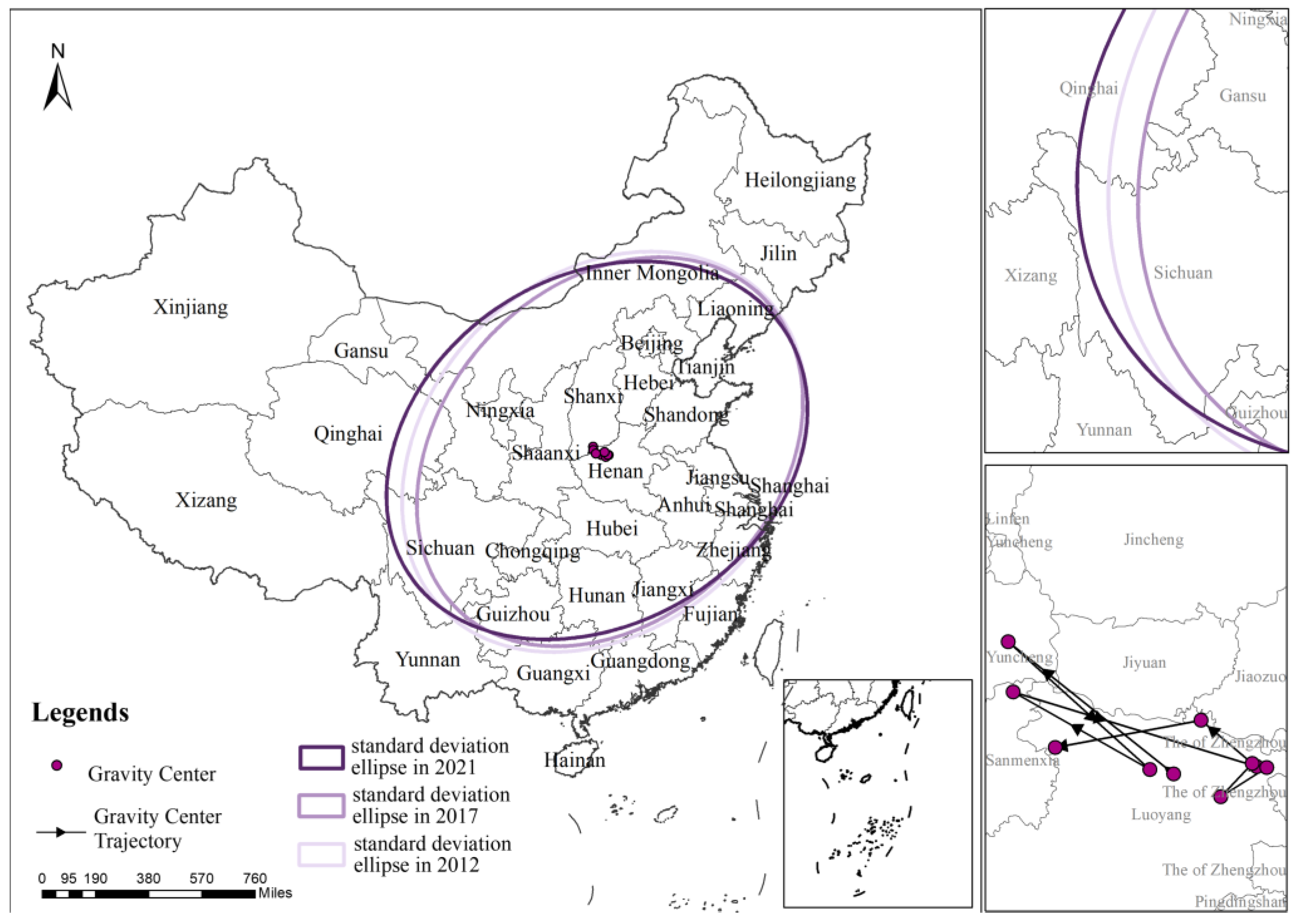
To capture the spatial dynamics of AGEE, this study employed the gravity centre-standard deviation ellipse model, a widely used approach for analysing geographical shifts under socio-economic and environmental influences. ArcGIS was applied to trace. AGEE’s spatial distribution evolution across China, with findings in

Table 6. Parameters of the standard deviation ellipse in AGEE.

Year	Length	Shape_Area	CenterY	CenterX	XStdDist	YStdDist	Distance
Unit	(km)	(104 km2)	(°E)	(°N)	(km)	(km)	(km)
2012	7262.199	408.018	112.463	34.740	1307.664	993.248	-
2013	7658.779	460.138	111.875	35.205	1334.616	1097.501	83.380
2014	7275.949	412.035	112.374	34.760	1293.691	1013.859	74.324
2015	7570.670	450.230	111.877	35.045	1313.801	1090.883	63.618
2016	7030.011	380.367	112.784	34.737	947.362	1278.091	106.352
2017	6984.649	375.544	112.821	34.731	1269.426	941.735	4.195
2018	6854.174	364.269	112.635	34.653	1228.683	943.749	22.412
2019	6942.588	372.328	112.767	34.748	1253.777	945.323	18.091
2020	6910.238	370.386	112.588	34.900	1237.810	952.521	26.129
2021	7212.816	401.367	112.020	34.858	1305.671	978.550	63.281

and Figure 4.

China’s AGEE was predominantly distributed along a northeast-southwest axis, as revealed by the standard deviation ellipse. The area of the ellipse first contracted and then expanded, indicating time-varying spatial heterogeneity. Along the major (X) axis, length first decreased and then increased, suggesting dispersion followed by reconcentration. Along the minor (Y) axis, length fluctuated—rising, then falling, and rising again—implying a “concentrated–dispersed–concentrated” process. Based on the centroid trajectory from 2012 to 2021, the centroid remained primarily in the central region, oscillating between Shanxi and Henan, and resided within Henan for most years. The centroid moved farther during 2012–2016 and less during 2017–2021, indicating that the spatial pattern of China’s agricultural production has remained relatively stable in recent years.

4.2. Dynamic Analysis of AGEE

The AGEE measures the efficiency of a DMU at a given point in relation to the production frontier surface, reflecting the relative efficiency level at a single point in time. Since agricultural production is a continuous process and production technology changes over time, introducing a green total factor productivity (GTP) index in the agricultural sector is crucial for capturing the dynamic development of AGEE.

4.2.1. The Value of GTP

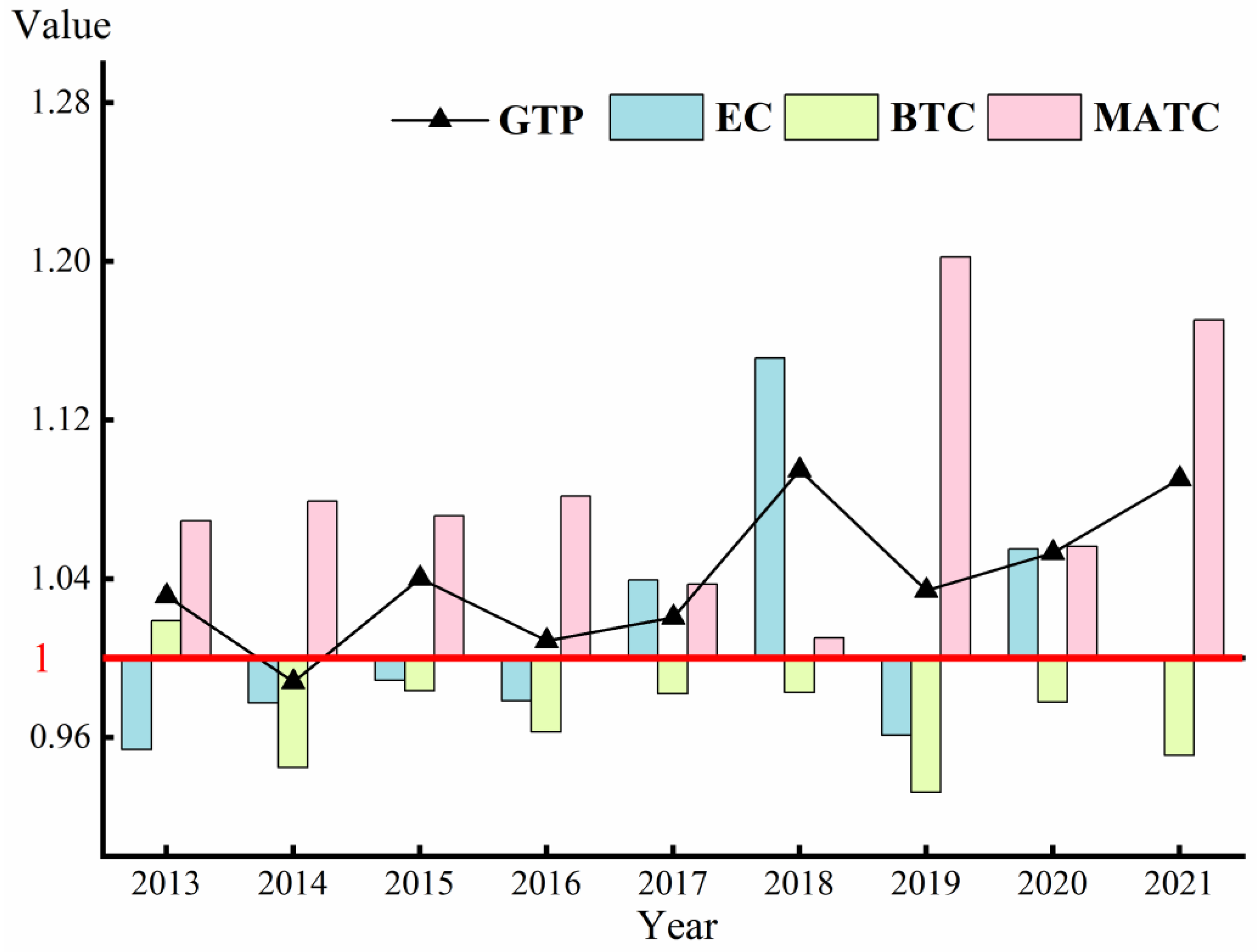
The value of China’s agricultural GTP and its index decomposition from 2013 to 2021 are shown in Figure 5. China’s agricultural GTP exceeded 1 in all years of the study period except 2014, indicating an overall upward trend in AGEE. Two distinct phases emerged in the progression of the EC index. During the first phase (2013–2016), the EC index remained below 1, suggesting a decline in technical efficiency that constrained AGEE growth. Resource misallocation may have contributed to this decline. In the second phase (2017–2021), the EC index exhibited significant fluctuations but remained above 1 on average, reflecting substantial improvements in technical efficiency that drove AGEE growth. However, reliance on efficiency gains alone poses risks of instability and unsustainability. Except for 2013, the BTC index remained below 1 throughout the study period, while the MATC consistently surpassed 1. This indicates that technological progress in Chinese agriculture was driven mainly by general-purpose technologies rather than green innovation. Furthermore, the MATC level was closely aligned with GTP, both fluctuating above 1, underscoring MATC as the primary driver of agricultural GTP.

In conclusion, China’s agricultural GTP remained consistently above 1 throughout the study period, signifying a sustained enhancement in AGEE. The decomposition analysis reveals that this improvement was predominantly attributable to technological progress, with limited contributions from technical efficiency, while technological innovation remains a major barrier.

4.2.2. Regional Differences in GTP

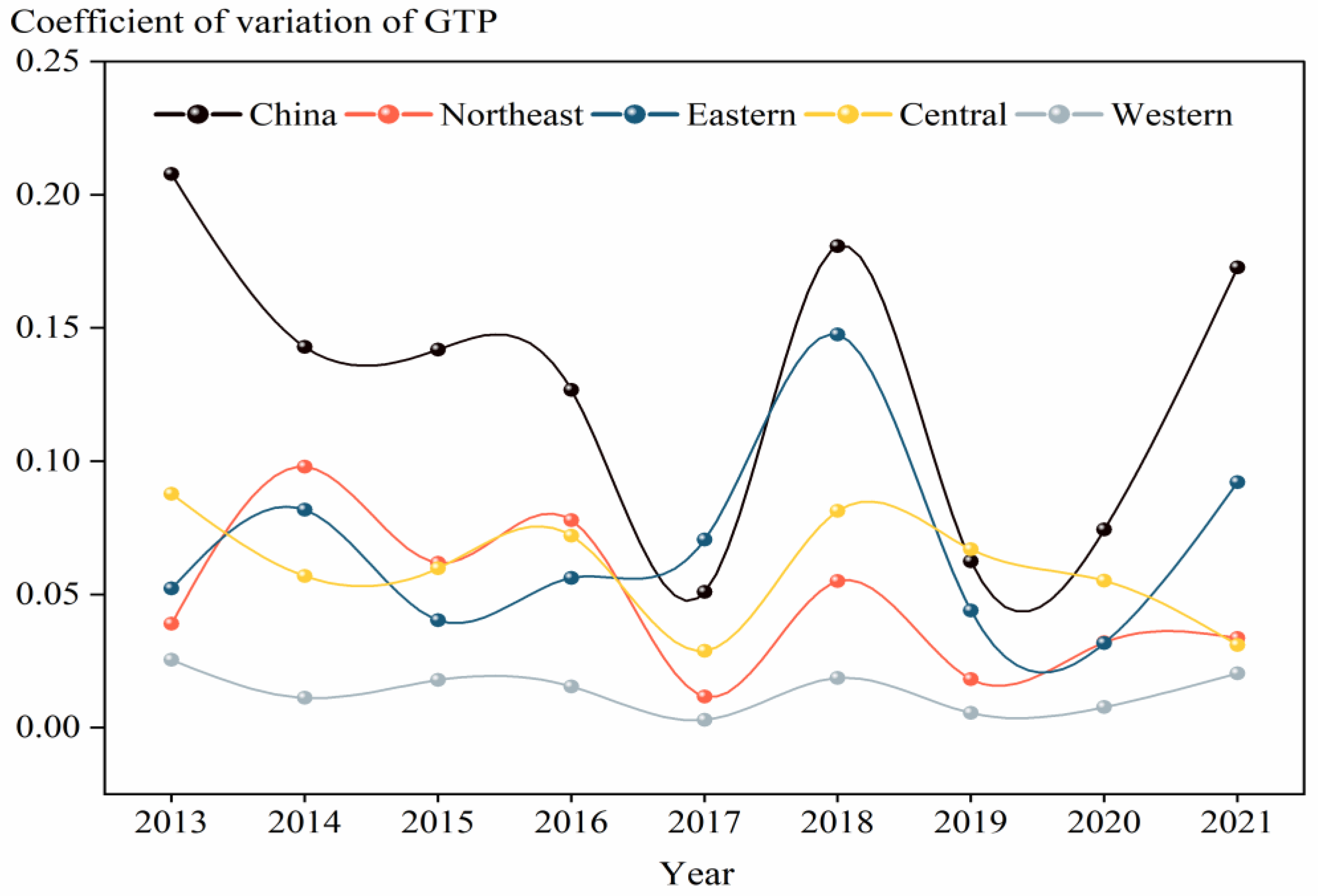
Although the aforementioned results confirmed the growth trend of AGEE and its primary sources, China’s agricultural resource endowments and technological development levels exhibit significant regional disparities. Therefore, further investigation of the regional distribution differences in agricultural GTP is necessary. This study further utilised the coefficient of variation (CV) to quantify the extent of variation in agricultural GTP values nationally and across economic regions, assessing the regional disparity and dynamic evolution of AGEE growth, and further employed t-tests to determine the statistical significance of the convergence or divergence trends, as presented in Figure 6.

As shown in Figure 6, the CV of China’s agricultural GTP peaked in 2013 at 20.78%, followed by a steady decline from 2013 to 2016. However, from 2017 to 2021, the CV fluctuated markedly. Statistical significance testing (t-test) confirmed a significant convergence trend at the national level prior to 2017 (|t| = 2.55 > |t|_{α = 0.05}), which became non-significant in the post-2017 period (|t| = 0.04 < |t|_{α = 0.05}). This pattern indicates that regional disparity in agricultural GTP initially converged and then diverged after 2017, reflecting an increasingly uneven spatial pattern in AGEE growth. By economic region, regional CVs were lower than the national average, with notable cross-region differences. This suggests that agricultural productivity is closely linked to climatic conditions, land resources, and agricultural technology. Notably, the West exhibited a substantially lower CV than other regions, suggesting lower production volatility and more even AGEE development. Furthermore, the northeastern region demonstrated a consistent year-over-year decline in CV of agricultural GTP, a trend that was statistically significant (|t| = 2.41 > |t|_{α = 0.05}). This aligns with China’s recent prioritisation of food security in this area, reflecting the successful implementation of policies and practices that have stabilised and improved agricultural productivity. After 2018, the central region also experienced a significant decline in CV (|t| = 8.62 > |t|_{α = 0.01}). However, the East experienced sharp fluctuations in CV after 2017 (|t| = 0.69 < |t|_{α = 0.05}), suggesting that as the green agricultural transition deepened, AGEE growth became increasingly unbalanced and volatile, underscoring the need for a more effective regional coordination mechanism. Moreover, regional CVs differed markedly year to year. For example, in 2018, the East recorded the highest CV in GTP (14.76%), whereas the Northeast and the West recorded 5.50% and 1.87%, respectively.

4.2.3. The Causes of Regional Differences in GTP

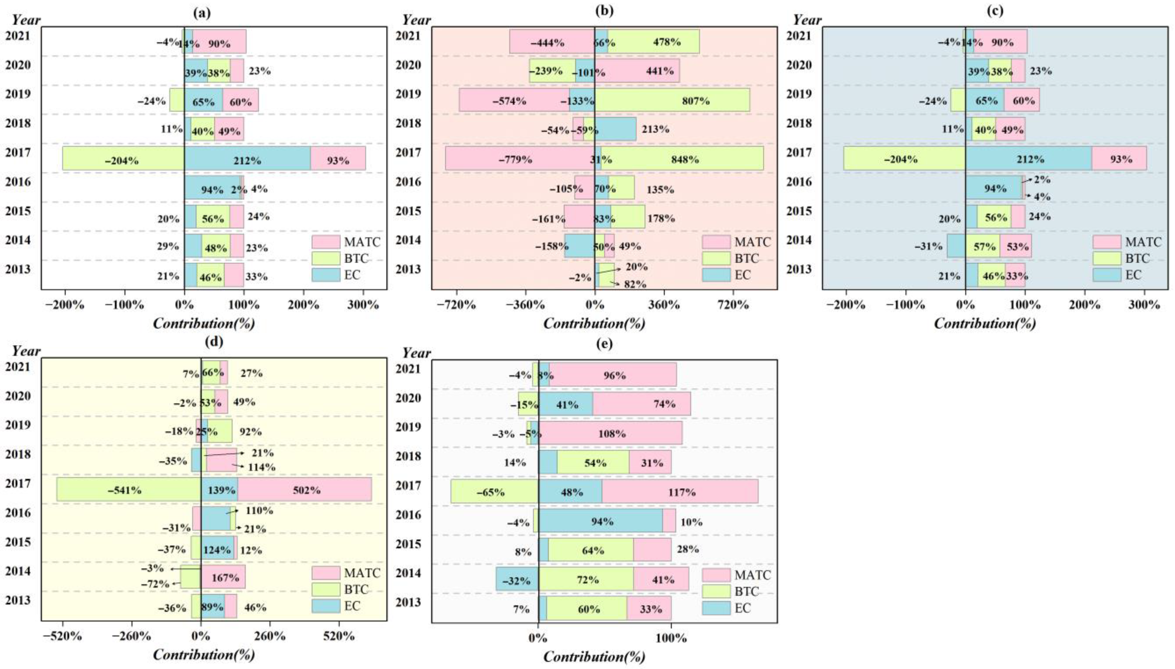
Given the pronounced regional differences in GTP across China and its major economic zones, it is imperative to investigate the primary cause behind the uneven growth of AGEE. The contribution of differences in each GTP decomposition term to the overall GTP disparities was measured using variance decomposition (Figure 7).

The underlying drivers of uneven growth in AGEE exhibited marked temporal and regional heterogeneity. As shown in Figure 7a, at the national level, the average contributions of EC, BTC, and MATC to spatial disparities in agricultural GTP were 55.95%, −0.29%, and 44.34%, respectively, indicating that EC and MATC were the main sources of regional differences in GTP. By subperiod, the contributions from all three components were positive from 2013 to 2015, with BTC being the largest. By 2015, BTC’s contribution had surged to 56.22%, with EC and MATC contributing roughly the same level. This suggests that technological advancements in green agriculture significantly boosted productivity in leading regions, widening the gap with lagging areas. In 2016–2017, the contribution of EC increased dramatically to 94.04% and 211.65%, respectively, whereas the contribution of BTC declined sharply. In particular, in 2017, BTC had a substantial negative contribution of –204.34% to GTP regional differences. This period made EC the dominant explanatory factor, indicating that differences in production processes, management practices, and the effectiveness of technology implementation primarily drove the imbalance in AGEE growth. Earlier gains from green technology entered a “digestion” phase, during which managerial-capacity differences became the core source of efficiency divergence. “From 2018 to 2021, MATC became the leading contributor (55.49%), followed by EC (32.09%), reflecting pronounced disparities in general-purpose frontier technologies—such as biological breeding and digital agriculture—emerging as a primary driver of regional development imbalances.

At the regional level, Figure 7b shows that BTC contributed strongly to GTP differences in the Northeast (mean 253.31%), whereas MATC acted as a suppressor (mean −181.09%). EC’s absolute contribution was smaller and highly volatile. These findings suggested that regional gaps in green agricultural technologies largely drove the uneven growth in AGEE in the Northeast. In the East (Figure 7c), all three components generally contributed positively to GTP disparities, with shifting dominance across subperiods. BTC played the leading role during 2013–2015, EC became the main contributor in 2016–2017, and from 2018 to 2021, MATC and EC contributed at comparable levels. This time-varying pattern was consistent with that observed at the national level. Temporal dynamics were also evident in the Central and West (Figure 7d,e): in the central region, EC, MATC, and BTC each dominated in different years, whereas in the West, disparities were driven mainly by BTC and MATC (except in 2016), with dominance shifting from BTC to MATC over time. These findings indicate that the structural causes of the uneven growth in AGEE vary significantly by region. For policymakers, tailoring flexible strategies to local resource endowments is essential to promoting high-level regional coordination in AGEE development.

4.2.4. AGEE Improvement Paths

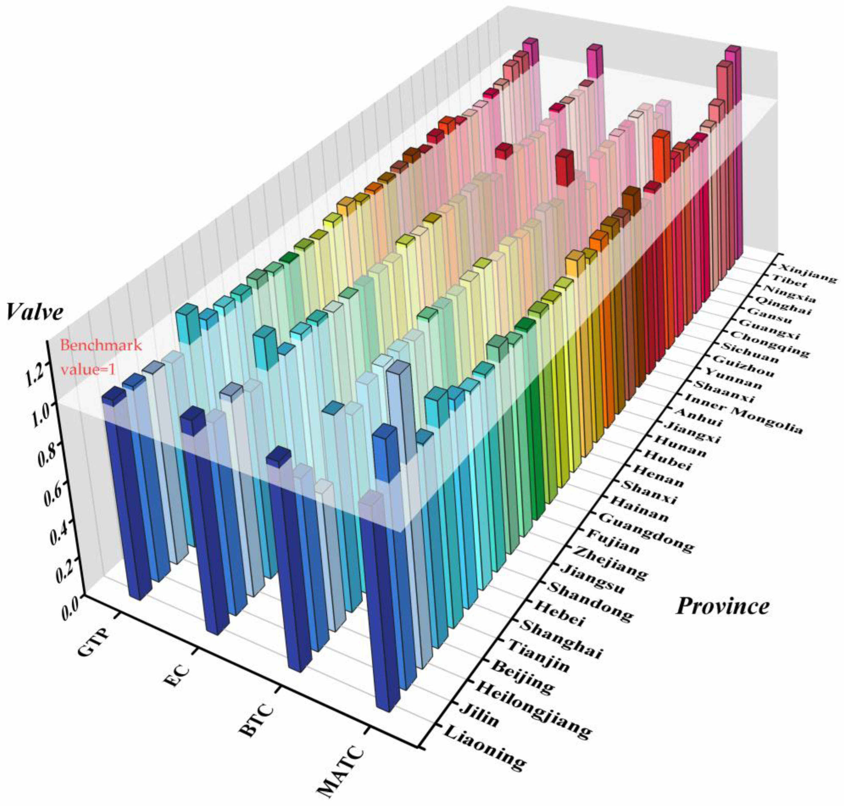
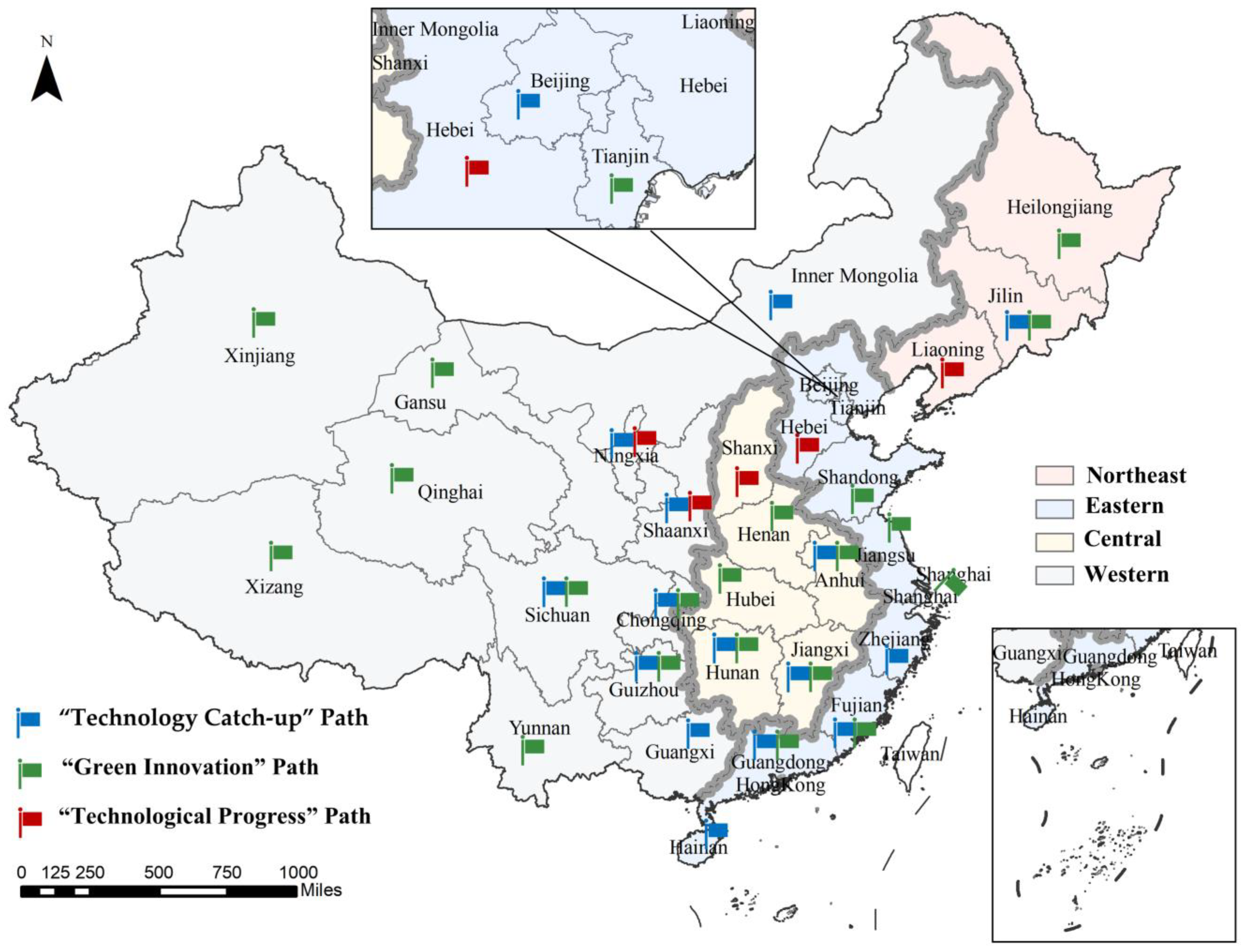
Based on analysing the growth of China’s AGEE and its distribution characteristics at the overall level, this study drew on the ideas of Lin and Bai [80] to determine the path of AGEE enhancement in each province based on the mean values of the EC, BTC, and MATC indices. Specifically, if a province’s EC, BTC, or MATC index is below 1.000, that index is considered a bottleneck factor restricting the enhancement of the province’s agricultural GTP. In such cases, future development strategies for the province should prioritise improvements in this index. Conversely, if all three indices were ≥1.000, we compared each with the national average and flagged any component below the national average as the priority for improvement. Accordingly, we identified three paths for AGEE enhancement: “Technology Catch-Up,” “Green Innovation,” and “Technological Progress”. Figure 8 presents the regional distribution of China’s agricultural GTP and its decomposition, while Figure 9 illustrates the spatial landscape of provincial AGEE improvement paths.

As shown in Figure 8, all provinces except Beijing recorded GTP values greater than 1, indicating AGEE experienced positive growth nationwide. More than half of the provinces exhibited EC values above the benchmark, while provinces such as Jilin, Beijing, Fujian, Guangdong, Hainan, Hunan, Jiangxi, Anhui, Inner Mongolia, Shaanxi, Guizhou, Sichuan, Chongqing, Guangxi, and Ningxia had EC values below 1. These provinces experienced constraints in AGEE improvement due to insufficient technical efficiency and should consider adopting the “Technology Catch-up” path tailored to their local contexts. For the BTC index, only nine provinces—Liaoning, Beijing, Hebei, Zhejiang, Shanxi, Hainan, Shaanxi, Guangxi, and Qinghai—surpassed the benchmark, while the majority of provinces scored below the national average. This finding suggests that inadequate green technology remained a major barrier to provincial AGEE improvement, underscoring the need to accelerate green-technology innovation.

Regarding MATC, most provinces outperformed the baseline, except for Liaoning and Shaanxi. Further analysis revealed that Hebei, Zhejiang, Shaanxi, and Qinghai also fell below the national average in terms of MATC, highlighting the necessity for these provinces to enhance the scaled application of agricultural technologies and to follow the “Technological Progress” path. The spatial layout in Figure 9 reveals pronounced regional heterogeneity in provincial AGEE paths. In western China, “Green Innovation” emerged as the optimal strategy for advancing sustainable agriculture. In the central, southwestern, and southeastern regions, simultaneous efforts in production management and green technology R&D were more appropriate. Notably, in each of the four major regions—Northeast, East, Central, and West—a few provinces needed to prioritise improvements in scaled technologies, indicating that strengthening interregional cooperation on agricultural technology could be a feasible policy direction.

4.3. Influencing Factors Analysis of AGEE

4.3.1. Spatial Correlation of AGEE

Table 7. Global autocorrelation Moran’s I index of China’s AGEE.

Year	Moran’s I	P	Z	Year	Moran’s I	P	Z
2012	0.2590	0.0014 ***	3.1864	2017	0.2283	0.0048 ***	2.8222
2013	0.2168	0.0065 ***	2.7239	2018	0.0380	0.4450	0.7639
2014	0.2248	0.0049 ***	2.8152	2019	0.0793	0.2282	1.2049
2015	0.2054	0.0099 ***	2.5781	2020	0.8296	0.5023	0.6708
2016	0.2485	0.0022 ***	3.0570	2021	−0.0303	0.9738	0.6328

Note: *** indicates significance at the 1% significance level.

presents results derived from the global Moran’s I statistic, which was used to evaluate spatial association in AGEE among 31 Chinese provinces during the period 2012–2021.

As shown in Table 7, except in 2021, Moran’s I consistently showed positive values during the observation period, suggesting that agricultural green ecological efficiency (AGEE) exhibited significant positive spatial autocorrelation across the 31 provinces of China. In terms of significance, AGEE’s Moran’s I remained statistically significant from 2012 to 2017, indicating a stable and persistent spatial autocorrelation in AGEE. Between 2018 and 2021, however, the global Moran’s I statistic did not exhibit statistically significant spatial correlation. However, this does not conclusively indicate the absence of spatial autocorrelation in AGEE; further verification through local autocorrelation analysis was required.

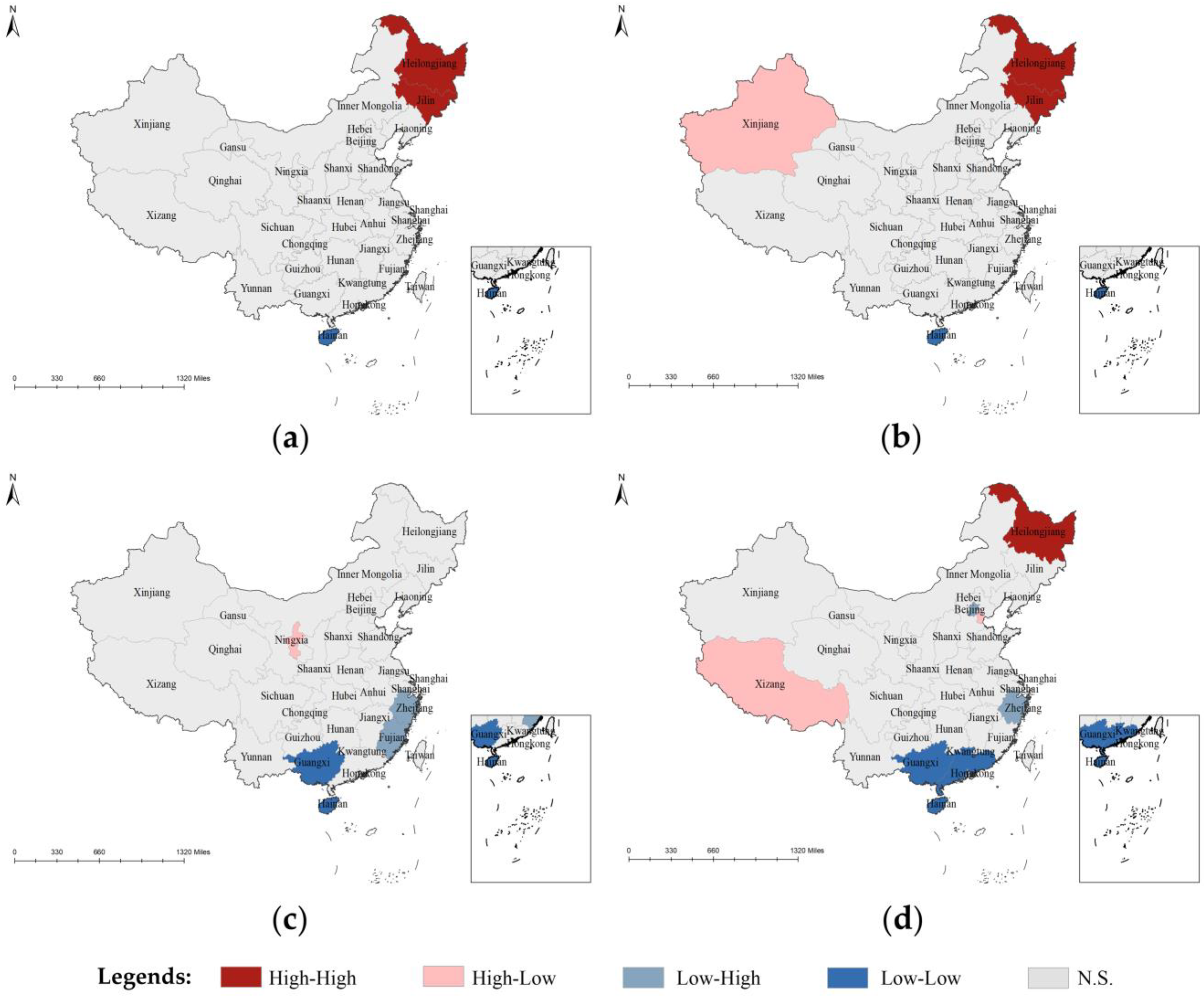
To further examine the provincial-level clustering patterns of AGEE, local spatial analysis was applied, and LISA cluster maps were produced for 2012, 2015, 2018, and 2021 to visualise localised spatial autocorrelation across the 31 Chinese provinces. (Figure 10).

During the study period, spatial correlations in AGEE among provinces were initially limited but increased over time, indicating a growing synergy in AGEE across Chinese provinces. In 2012, only three provinces demonstrated spatial correlations: Heilongjiang and Jilin exhibited a “high-high” agglomeration, while Hainan showed a “low-low” agglomeration. By 2015, Xinjiang joined with a “high-low” agglomeration. The number of provinces with spatial correlation rose to five by 2018, with Ningxia forming a ‘high-low’ agglomeration, Zhejiang and Fujian a ‘low-high’ agglomeration, and Guangxi and Hainan continuing as ‘low-low’ agglomeration. By 2021, the count had risen to eight provinces, with Heilongjiang displaying a “high-high” agglomeration, Tibet and Tianjin showing a “high-low” agglomeration, Zhejiang and Hebei demonstrating a “low-high” agglomeration, and Guangxi, Guangdong, and Hainan continuing with a “low-low” agglomeration. In addition, considering the spatial landscape, a notable AGEE high-value agglomeration phenomenon was observed in the northeast region, while the southern region was more likely to experience the mutual influence of low-level AGEE. Zhejiang and Fujian were negatively affected by the high-level AGEE in surrounding areas, primarily due to the prevalence of mountainous and forested areas, as well as less cultivated land. Moreover, the western regions were more likely to experience resource siphoning, resulting in a few areas exhibiting relative leadership.

4.3.2. The Analysis of Factors Influencing AGEE

In light of the observed local spatial autocorrelation of AGEE across provinces, this study further adopted a spatial econometric approach to investigate its driving factors and associated spillover effects.

Table 8. Spatial econometric model test results.

Test Content	Statistic	Statistical Value	Test Result
LM test	Moran’s I	−0.23	Rejection of the hypothesis that there is no spatial error between variables
	LM-error	0.283 *
	Robust LM-error	3.139 **
	LM-lag	0.059	Reject the hypothesis that there is no spatial lag between variables
	Robust LM-lag	2.915 *
Hausman test	Hausman	66.24 ***	Reject the hypothesis of significant difference in coefficients
LR test	LR-lag	20.59 ***	Reject SDM degradation to SAR
	LR-error	19.40 ***	Reject SDM degradation to SEM
Wald test	Wald-lag	21.20 ***	Reject SDM degradation to SAR
	Wald-error	19.80 **	Reject SDM degradation to SEM

Note: *, ** and *** indicate significance at the 10%, 5% and 1% significance levels, respectively.

reports the outcomes of LM, Hausman, LR, and Wald tests, based on which the spatial Durbin specification with time-fixed was selected as the most suitable model.

Table 9. Factors influencing AGEE and spatial econometric analysis results.

Variables	Regression Coefficient	Lag Term Coefficient	Direct Effect	Spillover Effect	Total Effect
Spatial regression coefficient	−0.241 ***
Agriculture, forestry and water services ratio	−0.248	−0.676	−0.211	−0.463	−0.674
Aging rate	1.214	0.080	1.183	−0.050	1.134
Urbanization rate	0.095	−0.268	0.130	−0.271	−0.140
Industrial structure	−0.499 *	0.116	−0.511 **	0.249	−0.263
Disaster-affected rate	−0.019	−0.244	−0.010	−0.211	−0.220 **
Rural per capita disposable income	0.705 ***	−0.177	0.726 ***	−0.261	0.465
Effective irrigation rate	0.415 ***	0.865 ***	0.392 ***	0.659**	1.050 ***
Cultivation structure	0.983 ***	−0.550	1.003 ***	−0.659	0.344

Note: *, ** and *** indicate significance at the 10%, 5% and 1% significance levels, respectively.

presents insightful findings on the factors influencing AGEE and their spatial interdependence. Relying on the estimated coefficients from the spatial Durbin model, this study employed partial differentiation to disentangle each variable’s impact into direct and spatial spillover components, offering a holistic view of the variables’ influence on AGEE across regions. The spatial regression coefficient was significant at the 1% level. It marked −0.241, indicating that an increase in AGEE in neighbouring regions would harm the region, which might be attributed to the fact that agricultural production is essentially a competition for resources. With increasing environmental pressures, the competition for resources in agricultural production is intensifying in various regions. For example, agricultural development in neighbouring regions may lead to competition for water resources, thus affecting agricultural efficiency in the region.

The agricultural, forestry, and water services ratio, as well as the ageing and urbanisation rates, positively affected AGEE, while the affairs of the agricultural, forestry, and water services harmed AGEE. However, they did not meet statistical significance criteria. The advanced industrial structure had a significantly negative direct effect on AGEE. This adverse effect can be attributed to the “resource crowding effect” and the “population siphoning effect,” wherein resources and labour are shifted from agriculture to more profitable industrial sectors, posing challenges to agricultural productivity and ecological sustainability. This effect was predominantly localised due to the immediate impact of industrial activities within the province, while the spillover effects on neighbouring provinces were minimal. Possible explanations include delayed diffusion of economic activities, limited cross-regional resource flows, or divergent economic development strategies and industrial bases among provinces. However, the rural disposable income per capita had a positive effect on AGEE, with a direct effect of 0.726, which was significant at the 1% level. This finding suggests that higher incomes enabled farmers to adopt more efficient land-use practices, thereby enhancing land productivity while preserving the ecological environment. Such investments might have included land improvement and strategic planning. However, due to the immobility of land resources, the positive impact of disposable income was limited to the local AGEE. The significantly positive direct and spillover effects of adequate irrigation underscore its vital role in promoting AGEE within and beyond the local region. This may stem from improved irrigation infrastructure, which enhances soil quality, facilitates nutrient cycles, supports groundwater recharge, and mitigates salinisation—all of which create favourable conditions for crop growth. At the same time, this effect was persistent, cumulative, and diffuse, so the spatial effect on the AGEE became more significant as the coverage of the irrigation system expanded. Lastly, the cropping structure had a significant positive effect only on the local AGEE, suggesting that optimising cropping patterns directly contributes to enhancing local AGEE. Furthermore, after controlling for potential endogeneity, our core findings remain consistent and robust (Considering that variables such as rural per capita disposable income may have bidirectional causality with AGEE, this study follows previous research and employs the Han-Phillips Generalized Method of Moments (GMM) for endogeneity testing. This method effectively addresses potential endogeneity biases that may arise during the implementation of the spatial Durbin model. We would like to thank the reviewer for their valuable suggestion).

5. Discussion and Policy Insights

5.1. Optimising the AGEE Accounting Framework

Assessing agricultural green ecological efficiency (AGEE) is crucial because it offers detailed insights into the status of sustainable agricultural development and informs regional planning and policymaking [17]. Unlike many other human activities, agricultural production not only entails inevitable ecological costs but also generates substantial ecological benefits, as evidenced by Costanza et al. (1997) [56] and Alcon et al. (2024) [81]. Accordingly, the output side of efficiency analysis should capture both positive and negative ecological externalities to reflect the actual state of sustainable agriculture. Our results showed that, within an accounting framework that simultaneously includes agricultural carbon emissions and ESV, the computed AGEE ranged from 0.5 to 0.7, markedly higher than estimates from studies that considered carbon emissions alone [82], indicating that neglecting ESV leads to an underestimation of actual sustainable agricultural performance and underscoring the necessity of integrating ESV into efficiency analyses. Policymakers should objectively and comprehensively recognise the multifunctional nature of agriculture, integrate ESV into agricultural performance assessment and policy appraisal systems to better reconcile long-term ecological benefits with short-term economic returns. Additionally, enhancing farmers’ awareness of ecosystem services and providing them with incentives or subsidies can motivate the preservation and improvement of agroecosystem services.

Building on rigorous AGEE accounting, we further characterised China’s spatiotemporal patterns. Overall, AGEE exhibited a fluctuating upward trend during the study period, but the average level remained modest, indicating ample room for improvement. Among all regions, Northeast China recorded the highest AGEE, whereas the East lagged, broadly consistent with Kuang et al. (2020) [83] and Li et al. (2022) [32]. The high AGEE in the northeast can be attributed to its abundant land resources and high degree of large-scale operation, which not only support high grain output but also contribute to ecosystem services such as water retention, soil conservation, and carbon sequestration [84]. In contrast, high urbanization and industrialization in Eastern China have intensified competition for land, water, and labor, leading to land fragmentation and a weakened labor force, which in turn reduces agricultural ecosystem services. The region’s heavy reliance on chemical inputs has exacerbated environmental problems [85,86,87]. Therefore, policymakers should implement region-specific strategies: the northeast should further exploit its potential in carbon sequestration and emission reduction while maintaining advantages in scale and organisational efficiency, whereas the Eastern region must prioritise spatial planning and factor reallocation, strictly protect existing cropland resources, and shift from chemical-input-dependent production toward technology- and ecology-driven practices. Furthermore, kernel density estimation indicated a widening interregional disparity in AGEE, while directional distribution analysis revealed a relatively stable spatial pattern aligned along a northeast–southwest axis centered on Henan and Shanxi provinces. In response, we recommend enhancing interregional cooperation mechanisms for agricultural green development, establishing a cross-regional green agriculture community along this axis, and facilitating efficient flows and allocation of knowledge, technology, talent, and green production factors.

5.2. Understanding the Dynamics of AGEE

From a developmental perspective, achieving sustained growth and regional equity in AGEE is crucial. Dynamic analysis results showed that the growth rate of AGEE (GTP) generally remained above 1, but at a low level. MATC was the primary driver of this growth, while EC had a limited contribution, and BTC became the primary constraint. This pattern underscores the vital role of general-purpose technological progress—such as the adoption of improved crop varieties and digital agriculture—in enhancing agricultural production potential, while also highlighting significant shortcomings in green innovation. Lagging green innovation represents a major shortcoming. These findings align closely with those of Yang et al. (2022) [31]. Further analysis of equity revealed that, post-2017, the growth gap at the national level widened, primarily driven by MATC and EC. Regionally, growth in the West was more equitable, the Central and Northeast exhibited partial convergence, whereas the East experienced significant internal divergence.

Additionally, the mechanisms underlying growth imbalances were complex, with the dominant roles of EC, MATC, and BTC varying significantly over time and across regions. This suggests that relying solely on basic technological advancement cannot achieve inclusive AGEE development; imbalances in management capacity, institutional support, and green technology are contributing to growth inequality. At the national level, policymakers should increase R&D investment and promote the broad application of basic technologies such as biotechnology and smart agriculture, while embedding green technology incentives throughout agricultural production to gradually address the persistent lag in BTC. To mitigate regional imbalances, efforts should focus on enhancing agricultural extension services, improving digital infrastructure in less developed regions, and establishing cross-regional support partnerships to facilitate knowledge exchange—thereby reducing growth gaps stemming from uneven MATC and BTC. In the East, addressing the increasing disparities in agricultural growth requires implementing unified standards and platform-based services, alongside using incentives to foster the synergistic development and application of technological innovations. The Central and Northeast regions should maintain and expand convergence, addressing BTC-driven imbalances by equitably deploying energy-saving and emission-reduction technologies through subsidies and technical assistance. The western region should prioritise improving accessibility to infrastructure and general-purpose technologies to ensure that benefits from new varieties and digital tools reach all farmers.

Beyond overarching coordination, enhancing AGEE requires region-specific and tailored policy interventions [31]. Based on regional development conditions, this study identifies differentiated improvement paths for each province [21]. Provinces with low EC should prioritize “technology catch-up” to accelerate green transition and improve technical efficiency—optimizing the flow and allocation of land, labor, and capital toward efficient entities while strengthening management by standardizing and intensifying cooperatives and family farms. In provinces such as Jilin and Shaanxi, where MATC lagged, the focus should be on a “technological progress” strategy—scaling R&D in agricultural technologies, promoting foundational innovations, and systematically enhancing production potential; balanced allocation of technological resources and east–west research collaboration should also be advanced to enable leapfrogging in less-developed areas. Because more than 70% of provinces fell behind in BTC, “green innovation” must be prioritized: expand the supply and adoption of green agricultural technologies, establish collaborative systems to support breakthroughs in emission reduction, carbon sequestration, resource conservation, and ecological protection, and refine incentive policies—such as green finance and eco-compensation—to spur uptake of green inputs and low-carbon practices and to accelerate diffusion of innovations.

5.3. Exploring the Spatial Influencing Factors of AGEE

An exploratory spatial analysis of AGEE at the provincial level revealed that, although the number of provinces with spatial correlation in agricultural green ecological efficiency decreased during the study period, the number of significant provinces increased over time, indicating that the spatial effect among Chinese provinces is becoming more pronounced. Analysis of the AGEE’s influencing factors revealed that rural per capita disposable income, effective irrigation rate, and the optimisation of cropping structure had positive effects, whereas a more advanced industrial structure was associated with adverse impacts. Research indicates that higher income levels among rural residents lead to a heightened preference for environmentally sustainable food products [88]. This shift in consumer demand encourages farmers to adopt more sustainable agricultural practices, aligning their production methods with the growing market demand for green food. In addition, higher incomes will also improve farmers’ living conditions, enabling them to pay more attention to long-term environmental quality and ecological balance. Increasing the effective irrigation rate can ensure crop irrigation while minimising water resource waste. Optimising cropping structures can also increase food production [65] and enhance agroecosystem services [89]. Therefore, advancing agricultural modernisation and refining cropping strategies, anchored in the twin pillars of food and ecological security, is imperative to ensure sustainable growth. Moreover, fostering synergies and collaboration across regions is crucial for enhancing agroecological efficiency. This involves crafting tailored agricultural development strategies, creating frameworks for regional cooperation, and facilitating the exchange of technology and resources between provinces to collectively elevate the standard of green agriculture. Regarding industrial structure, ensuring a more equitable allocation of resources is essential so that agriculture secures sufficient financial, technological, and human support during the upgrading process.

6. Research Limitations

This study developed a comprehensive framework that integrates carbon emissions and ecosystem service value (ESV) to evaluate Agricultural Green Ecological Efficiency (AGEE) in China, employing diverse methods to analyse its growth, equity, mechanisms, and spatial influences. The results offer important insights for sustainable agricultural policy and regional coordination.

Nonetheless, several limitations remain:

(1)

The AGEE accounting model could be further augmented. While incorporating key ecological externalities, it omits natural inputs (e.g., solar, wind, soil, and water energy), other pollutants beyond CO₂ (e.g., air, water, and soil contaminants). Additionally, although biomass factors (CF) have been used to calibrate ESV across regions, further refinement can be made by considering the ecological function differences in various crops within each region, which would improve the inter-provincial comparability and policy targeting.

(2)

The study scale remains macro-oriented. Using provincial-level data, the findings inform broad regional strategies; however, they fail to capture micro-level dynamics at finer scales, such as counties or farms, where more actionable management insights could be derived.

(3)

The complex effects of socio-economic factors on AGEE warrant further investigation. While this study uses spatial econometric models to capture local and spillover effects, the results are constrained by linear and independent assumptions. In reality, impacts may be nonlinear, involve thresholds, or reflect interactions among factors. Future work should use advanced models to capture this heterogeneity and complexity.

References

1. Li, Z.; Jin, M.; Cheng, J. Economic growth of green agriculture and its influencing factors in china: Based on emergy theory and spatial econometric model. Environ. Dev. Sustain. 2021, 23, 15494–15512. [Google Scholar] [CrossRef]
2. Liu, M.; Fang, X.; Ren, J. Accelerating the modernization of agriculture and rural areas in China. China Agric. Econ. Rev. 2023, 15, 871–880. [Google Scholar] [CrossRef]
3. van Wesenbeeck, C.F.A.; Keyzer, M.A.; van Veen, W.C.M.; Qiu, H. Can China’s overuse of fertilizer be reduced without threatening food security and farm incomes? Agric. Sys. 2021, 190, 103093. [Google Scholar] [CrossRef]
4. Lin, L.; Gu, T.; Shi, Y. The influence of new quality productive forces on high-quality agricultural development in China: Mechanisms and empirical testing. Agriculture 2024, 14, 1022. [Google Scholar] [CrossRef]
5. Zhu, X.; Zhang, Y.; Zhu, Y.; Li, Y.; Cui, J.; Yu, B. Multidimensional deconstruction and workable solutions for addressing China’s food security issues: From the perspective of sustainable diets. Land Use Pol. 2025, 148, 107401. [Google Scholar] [CrossRef]
6. Wang, J.; Dai, C. Identifying the spatial–temporal pattern of cropland’s non-grain production and its effects on food security in China. Foods 2022, 11, 3494. [Google Scholar] [CrossRef]
7. Jagtap, S.; Trollman, H.; Trollman, F.; Garcia-Garcia, G.; Parra-López, C.; Duong, L.; Martindale, W.; Munekata, P.E.; Lorenzo, J.M.; Hdaifeh, A. The Russia-Ukraine conflict: Its implications for the global food supply chains. Foods 2022, 11, 2098. [Google Scholar] [CrossRef]
8. Lee, C.-C.; Qian, A. Regional differences, dynamic evolution, and obstacle factors of cultivated land ecological security in China. Socioecon. Plann. Sci. 2024, 94, 101970. [Google Scholar] [CrossRef]
9. Liu, C.; Song, C.; Ye, S.; Cheng, F.; Zhang, L.; Li, C. Estimate provincial-level effectiveness of the arable land requisition-compensation balance policy in mainland China in the last 20 years. Land Use Pol. 2023, 131, 106733. [Google Scholar] [CrossRef]
10. Cheng, Z.; He, J.; Liu, Y.; Zhang, Q.; Deng, Y. Exploring the spatial structure and impact factors of water use efficiency in China. Environ. Impact Assess. Rev. 2023, 103, 107258. [Google Scholar] [CrossRef]
11. Zhang, Y.; Wang, J.; Fan, S. Healthy and Sustainable Diets in China and Their Global Implications. Agric. Econ. 2025, 56, 349–359. [Google Scholar] [CrossRef]
12. Yu, Y.; Hu, Y.; Gu, B.; Reis, S.; Yang, L. Reforming smallholder farms to mitigate agricultural pollution. Environ. Sci. Pollut. R 2022, 29, 13869–13880. [Google Scholar] [CrossRef]
13. Laurett, R.; Paço, A.; Mainardes, E.W. Sustainable Development in Agriculture and its Antecedents, Barriers and Consequences—An Exploratory Study. Sustain. Prod. Consum. 2021, 27, 298–311. [Google Scholar] [CrossRef]
14. Pretty, J.; Bharucha, Z.P. Sustainable intensification in agricultural systems. Ann. Bot. 2014, 114, 1571–1596. [Google Scholar] [CrossRef]
15. Guo, S.; Hu, Z.; Ma, H.; Xu, D.; He, R. Spatial and temporal variations in the ecological efficiency and ecosystem service value of agricultural land in China. Agriculture 2022, 12, 803. [Google Scholar] [CrossRef]
16. Zhang, R.; Zhang, L.; He, M.; Wang, Z. Spatial Association Network and Driving Factors of Agricultural Eco-Efficiency in the Hanjiang River Basin, China. Agriculture 2023, 13, 1172. [Google Scholar] [CrossRef]
17. Wang, J.; Su, D.; Wu, Q.; Li, G.; Cao, Y. Study on eco-efficiency of cultivated land utilization based on the improvement of ecosystem services and emergy analysis. Sci. Total Environ. 2023, 882, 163489. [Google Scholar] [CrossRef]
18. Zhuang, M.; Wang, X.; Yang, Y.; Wu, Y.; Wang, L.; Lu, X. Agricultural machinery could contribute 20% of total carbon and air pollutant emissions by 2050 and compromise carbon neutrality targets in China. Nat. Food 2025, 6, 513–522. [Google Scholar] [CrossRef] [PubMed]
19. Song, S.; Zhao, S.; Zhang, Y.; Ma, Y. Carbon Emissions from Agricultural Inputs in China over the Past Three Decades. Agriculture 2023, 13, 919. [Google Scholar] [CrossRef]
20. Li, M.; Li, F.; Qiu, J.; Zhou, H.; Wang, H.; Lu, H.; Zhang, N.; Song, Z. Multi-objective optimization of non-fossil energy structure in China towards the carbon peaking and carbon neutrality goals. Energy 2024, 312, 133643. [Google Scholar] [CrossRef]
21. Han, H.; Yang, X. Agricultural tridimension pollution emission efficiency in China: An evaluation system and influencing factors. Sci. Total Environ. 2024, 906, 167782. [Google Scholar] [CrossRef]
22. Tao, J.; Lu, Y.; Ge, D.; Dong, P.; Gong, X.; Ma, X. The spatial pattern of agricultural ecosystem services from the production-living-ecology perspective: A case study of the Huaihai Economic Zone, China. Land Use Pol. 2022, 122, 106355. [Google Scholar] [CrossRef]
23. Zabala, J.A.; Martínez-Paz, J.M.; Alcon, F. A comprehensive approach for agroecosystem services and disservices valuation. Sci. Total Environ. 2021, 768, 144859. [Google Scholar] [CrossRef]
24. Kulak, M.; Graves, A.; Chatterton, J. Reducing greenhouse gas emissions with urban agriculture: A Life Cycle Assessment perspective. Landsc. Urban Plann. 2013, 111, 68–78. [Google Scholar] [CrossRef]
25. Lin, B.B.; Philpott, S.M.; Jha, S. The future of urban agriculture and biodiversity-ecosystem services: Challenges and next steps. Basic Appl. Ecol. 2015, 16, 189–201. [Google Scholar] [CrossRef]
26. Clucas, B.; Parker, I.D.; Feldpausch-Parker, A.M. A systematic review of the relationship between urban agriculture and biodiversity. Urban Ecosyst. 2018, 21, 635–643. [Google Scholar] [CrossRef]
27. Park, H.; Kramer, M.; Rhemtulla, J.M.; Konijnendijk, C.C. Urban food systems that involve trees in Northern America and Europe: A scoping review. Urban For. Urban Green. 2019, 45, 126360. [Google Scholar] [CrossRef]
28. Hsu, S.-Y.; Yang, C.-Y.; Chen, Y.-L.; Lu, C.-C. Agricultural efficiency in different regions of china: An empirical analysis based on dynamic sbm-DEA model. Sustainability 2023, 15, 7340. [Google Scholar] [CrossRef]
29. Lei, S.; Yang, X.; Qin, J. Does agricultural factor misallocation hinder agricultural green production efficiency? Evidence from China. Sci. Total Environ. 2023, 891, 164466. [Google Scholar] [CrossRef]
30. Liao, J.; Yu, C.; Feng, Z.; Zhao, H.; Wu, K.; Ma, X. Spatial differentiation characteristics and driving factors of agricultural eco-efficiency in Chinese provinces from the perspective of ecosystem services. J. Clean Prod. 2021, 288, 125466. [Google Scholar] [CrossRef]
31. Yang, H.; Wang, X.; Bin, P. Agriculture carbon-emission reduction and changing factors behind agricultural eco-efficiency growth in China. J. Clean Prod. 2022, 334, 130193. [Google Scholar] [CrossRef]
32. Li, S.; Zhu, Z.; Dai, Z.; Duan, J.; Wang, D.; Feng, Y. Temporal and Spatial Differentiation and Driving Factors of China’s Agricultural Eco-Efficiency Considering Agricultural Carbon Sinks. Agriculture 2022, 12, 1726. [Google Scholar] [CrossRef]
33. Liu, Y.; Zou, L.; Wang, Y. Spatial-temporal characteristics and influencing factors of agricultural eco-efficiency in China in recent 40 years. Land Use Pol. 2020, 97, 104794. [Google Scholar] [CrossRef]
34. Zhao, X.; Yang, J.; Chen, H.; Zhang, X.; Xi, Y. The effect of urbanization on agricultural eco-efficiency and mediation analysis. Front. Environ. Sci. 2023, 11, 1199446. [Google Scholar] [CrossRef]
35. Gao, L.; Zhao, G.; Liang, L.; Chen, B. Achieving higher eco-efficiency for three staple food crops with ecosystem services based on regional heterogeneity in China. Sci. Total Environ. 2024, 948, 174942. [Google Scholar] [CrossRef]
36. Verfaillie, H.A.; Bidwell, R. Measuring Eco-Efficiency: A Guide to Reporting Company Performance; World Business Council for Sustainable Development: Geneva, Switzerland, 2000; ISBN 2-940240-14-0. Available online: https://www.gdrc.org/sustbiz/measuring.pdf (accessed on 1 September 2025).
37. Paes, M.X.; de Medeiros, G.A.; Mancini, S.D.; Gasol, C.; Pons, J.R.; Durany, X.G. Transition towards eco-efficiency in municipal solid waste management to reduce GHG emissions: The case of Brazil. J. Clean Prod. 2020, 263, 121370. [Google Scholar] [CrossRef]
38. Xu, T.; Umair, M.; Cheng, W.; Hakimova, Y.; Mang, G. Evaluating Eco-Efficiency as a metric for sustainable urban Growth: A comparative study of provincial capital cities in China. Ecol. Indic. 2024, 169, 112959. [Google Scholar] [CrossRef]
39. Mounmemi, M.; Mohammadou, N.; Kobou, G. Does woodfuel price distortion inhibit eco-efficiency in woodfuel exploitation systems in sub-saharan africa? Evidence from cameroon. Clim. Change Econ. 2023, 15, 2340008. [Google Scholar] [CrossRef]
40. You, J.; Hu, J.; Jiang, B. The correlation evolution and formation mechanism of energy ecological efficiency in China: A spatial network approach. Energy 2024, 313, 133971. [Google Scholar] [CrossRef]
41. Waltersmann, L.; Kiemel, S.; Stuhlsatz, J.; Sauer, A.; Miehe, R. Artificial Intelligence Applications for Increasing Resource Efficiency in Manufacturing Companies—A Comprehensive Review. Sustainability 2021, 13, 6689. [Google Scholar] [CrossRef]
42. Garnett, T.; Appleby, M.C.; Balmford, A.; Bateman, I.J.; Benton, T.G.; Bloomer, P.; Burlingame, B.; Dawkins, M.; Dolan, L.; Fraser, D.; et al. Sustainable Intensification in Agriculture: Premises and Policies. Science 2013, 341, 33–34. [Google Scholar] [CrossRef]
43. Myeki, L.W.; Matthews, N.; Bahta, Y.T. Decomposition of Green Agriculture Productivity for Policy in Africa: An Application of Global Malmquist–Luenberger Index. Sustainability 2023, 15, 1645. [Google Scholar] [CrossRef]
44. Jin, B.; Cui, C.; Wen, L.; Shi, R.; Zhao, M. Regional differences and convergence of agricultural carbon efficiency in China: Embodying carbon sink effect. Ecol. Indic. 2024, 169, 112929. [Google Scholar] [CrossRef]
45. Ge, P.; Liu, T.; Wu, X.; Huang, X. Heterogenous Urbanization and Agricultural Green Development Efficiency: Evidence from China. Sustainability 2023, 15, 5682. [Google Scholar] [CrossRef]
46. Baum, R.; Bieńkowski, J. Eco-Efficiency in Measuring the Sustainable Production of Agricultural Crops. Sustainability 2020, 12, 1418. [Google Scholar] [CrossRef]
47. Cao, X.; Zeng, W.; Wu, M.; Li, T.; Chen, S.; Wang, W. Water resources efficiency assessment in crop production from the perspective of water footprint. J. Clean Prod. 2021, 309, 127371. [Google Scholar] [CrossRef]
48. Godoy-Durán, Á.; Galdeano- Gómez, E.; Pérez-Mesa, J.C.; Piedra-Muñoz, L. Assessing eco-efficiency and the determinants of horticultural family-farming in southeast Spain. J. Environ. Manag. 2017, 204, 594–604. [Google Scholar] [CrossRef] [PubMed]
49. Đokić, D.; Novaković, T.; Tekić, D.; Matkovski, B.; Zekić, S.; Milić, D. Technical Efficiency of Agriculture in the European Union and Western Balkans: SFA Method. Agriculture 2022, 12, 1992. [Google Scholar] [CrossRef]
50. Tone, K. A strange case of the cost and allocative efficiencies in DEA. J. Oper. Res. Soc. 2002, 53, 1225–1231. [Google Scholar] [CrossRef]
51. Cui, Y.; Khan, S.U.; Deng, Y.; Zhao, M.; Hou, M. Environmental improvement value of agricultural carbon reduction and its spatiotemporal dynamic evolution: Evidence from China. Sci. Total Environ. 2021, 754, 142170. [Google Scholar] [CrossRef]
52. Huang, X.; Feng, C.; Qin, J.; Wang, X.; Zhang, T. Measuring China’s agricultural green total factor productivity and its drivers during 1998–2019. Sci. Total Environ. 2022, 829, 154477. [Google Scholar] [CrossRef]
53. Wang, B.; Zhang, W. Cross-provincial differences in determinants of agricultural eco-efficiency in China: An analysis based on panel data from 31 provinces in 1996–2015. China Rural. Econ. 2018, 17, 46–62. [Google Scholar]
54. Chi, M.; Guo, Q.; Mi, L.; Wang, G.; Song, W. Spatial Distribution of Agricultural Eco-Efficiency and Agriculture High-Quality Development in China. Land 2022, 11, 722. [Google Scholar] [CrossRef]
55. Yu, H.; Wei, Y. Measurement, Dynamic Evolution, and Spatial Convergence of the Efficiency of the Green and Low-Carbon Utilization of Cultivated Land Under the Goal of Food and Ecological “Double Security”: Empirical Evidence from the Huaihe River Ecological Economic Belt of China. Sustainability 2025, 17, 7242. [Google Scholar] [CrossRef]
56. Costanza, R.; d’Arge, R.; de Groot, R.; Farber, S.; Grasso, M.; Hannon, B.; Limburg, K.; Naeem, S.; O’Neill, R.V.; Paruelo, J.; et al. The value of the world’s ecosystem services and natural capital. Nature 1997, 387, 253–260. [Google Scholar] [CrossRef]
57. Song, M.; An, M.; He, W.; Wu, Y. Research on land use optimization based on PSO-GA model with the goals of increasing economic benefits and ecosystem services value. Sustain. Cities Soc. 2025, 119, 106072. [Google Scholar] [CrossRef]
58. Wang, T.; Wu, J.; Liu, J. Regional Differences, Dynamic Evolution, and Convergence of Global Agricultural Energy Efficiency. Agriculture 2024, 14, 1429. [Google Scholar] [CrossRef]
59. Chivu, L.; Andrei, J.V.; Zaharia, M.; Gogonea, R.-M. A regional agricultural efficiency convergence assessment in Romania—Appraising differences and understanding potentials. Land Use Pol. 2020, 99, 104838. [Google Scholar] [CrossRef]
60. Lei, Q.L. Yuelin Capital-Skill Complementarity and the Direction of Skill Bias of Technological Progress. Stat. Res. 2020, 37, 48–59. [Google Scholar]
61. Liu, W.; Du, M.; Bai, Y. Impact of environmental regulations on green total factor productivity. China Popul. Resour. Environ. 2022, 32, 95–107. [Google Scholar]
62. Gollin, D.; Udry, C. Heterogeneity, Measurement Error, and Misallocation: Evidence from African Agriculture. J. Political Econ. 2020, 129, 1–80. [Google Scholar] [CrossRef]
63. Li, H.; Zhou, X.; Tang, M.; Guo, L. Impact of Population Aging and Renewable Energy Consumption on Agricultural Green Total Factor Productivity in Rural China: Evidence from Panel VAR Approach. Agriculture 2022, 12, 715. [Google Scholar] [CrossRef]
64. Xie, G.; Xiao, Y.; Zhen, L.; Lu, C.; Zhang, C.; Zhang, L.; Chen, W.; Li, S. Improvement of ecosystem service valorization method based on unit area value equivalent factor. J. Nat. Resour. 2015, 30, 1243–1254. [Google Scholar]
65. Xie, G.; Xiao, Y.; Zhen, L. Study on ecosystem services value of food production in China. Chin. J. Eco-Agric. 2005, 13, 4. [Google Scholar]
66. Han, G.; Xu, J.; Zhang, X.; Pan, X. Efficiency and Driving Factors of Agricultural Carbon Emissions: A Study in Chinese State Farms. Agriculture 2024, 14, 1454. [Google Scholar] [CrossRef]
67. Hou, M.; Cui, X.; Xie, Y.; Lu, W.; Xi, Z. Synergistic emission reduction effect of pollution and carbon in China’s agricultural sector: Regional differences, dominant factors, and their spatial-temporal heterogeneity. Environ. Impact Assess. Rev. 2024, 106, 107543. [Google Scholar] [CrossRef]
68. Huang, J.; Lu, H.; Du, M. Regional Differences in Agricultural Carbon Emissions in China: Measurement, Decomposition, and Influencing Factors. Land 2025, 14, 682. [Google Scholar] [CrossRef]
69. Liu, G.; Deng, X.; Zhang, F. The spatial and source heterogeneity of agricultural emissions highlight necessity of tailored regional mitigation strategies. Sci. Total Environ. 2024, 914, 169917. [Google Scholar] [CrossRef]
70. Jing, X.; Tian, G.; Li, M.; Javeed, S.A. Research on the Spatial and Temporal Differences of China’s Provincial Carbon Emissions and Ecological Compensation Based on Land Carbon Budget Accounting. Int. J. Environ. Res. Public. Health 2021, 18, 12892. [Google Scholar] [CrossRef]
71. Feng, L.; Yang, W.; Hu, J.; Wu, K.; Li, H. Exploring the nexus between rural economic digitalization and agricultural carbon emissions: A multi-scale analysis across 1607 counties in China. J. Environ. Manag. 2025, 373, 123497. [Google Scholar] [CrossRef] [PubMed]
72. Tone, K. A slacks-based measure of efficiency in data envelopment analysis. Eur. J. Oper. Res. 2001, 130, 498–509. [Google Scholar] [CrossRef]
73. Färe, R.; Grosskopf, S.; Margaritis, D. Productivity Growth and Convergence in the European Union. J. Product. Anal. 2006, 25, 111–141. [Google Scholar] [CrossRef]
74. Jing, X.; Tao, S.; Hu, H.; Sun, M.; Wang, M. Spatio-temporal evaluation of ecological security of cultivated land in China based on DPSIR-entropy weight TOPSIS model and analysis of obstacle factors. Ecol. Indic. 2024, 166, 112579. [Google Scholar] [CrossRef]
75. Zhang, Q.; Yang, Y.; Li, X.; Wang, P. Digitalization and Agricultural Green Total Factor Productivity: Evidence from China. Agriculture 2024, 14, 1805. [Google Scholar] [CrossRef]
76. Guan, H.; Guo, B.; Zhang, J. Study on the Impact of the Digital Economy on the Upgrading of Industrial Structures—Empirical Analysis Based on Cities in China. Sustainability 2022, 14, 11378. [Google Scholar] [CrossRef]
77. Zheng, Y.; Wang, M.; Ma, X.; Zhu, C.; Gao, Q. The Dynamic Relationship Between Industrial Structure Upgrading and Carbon Emissions: New Evidence from Chinese Provincial Data. Sustainability 2024, 16, 10118. [Google Scholar] [CrossRef]
78. Fu, J.; Ding, R.; Zhu, Y.Q.; Du, L.Y.; Shen, S.W.; Peng, L.N.; Zou, J.; Hong, Y.X.; Liang, J.; Wang, K.X.; et al. Analysis of the spatial-temporal evolution of Green and low carbon utilization efficiency of agricultural land in China and its influencing factors under the goal of carbon neutralization. Environ. Res. 2023, 237, 116881. [Google Scholar] [CrossRef]
79. Cui, Y.; Khan, S.U.; Sauer, J.; Zhao, M. Exploring the spatiotemporal heterogeneity and influencing factors of agricultural carbon footprint and carbon footprint intensity: Embodying carbon sink effect. Sci. Total Environ. 2022, 846, 157507. [Google Scholar] [CrossRef]
80. Lin, B.; Bai, R. Dynamic energy performance evaluation of Chinese textile industry. Energy 2020, 199, 117388. [Google Scholar] [CrossRef]
81. Alcon, F.; Albaladejo-García, J.A.; Martínez-García, V.; Rossi, E.S.; Blasi, E.; Lehtonen, H.; Martínez-Paz, J.M.; Zabala, J.A. Cost benefit analysis of diversified farming systems across Europe: Incorporating non-market benefits of ecosystem services. Sci. Total Environ. 2024, 912, 169272. [Google Scholar] [CrossRef] [PubMed]
82. Zhang, H. Evaluation and analysis of spatio-temporal evolution trend of agricultural eco-efficiency in China. Agric. Ind. 2025, 7, 152–156. [Google Scholar]
83. Kuang, B.; Lu, X.; Zhou, M.; Chen, D. Provincial cultivated land use efficiency in China: Empirical analysis based on the SBM-DEA model with carbon emissions considered. Technol. Forecast. Soc. Change 2020, 151, 119874. [Google Scholar] [CrossRef]
84. Xiong, C.; Xu, H.; Tian, Y. Assessment of ecosystem service value in China from the perspective of spatial heterogeneity. Ecol. Indic. 2024, 159, 111707. [Google Scholar] [CrossRef]
85. Li, R.; Cui, W. Spatial–Temporal Evolution and Influencing Factors of Arable Land Green and Low-Carbon Utilization in the Yangtze River Delta from the Perspective of Carbon Neutrality. Sustainability 2024, 16, 6889. [Google Scholar] [CrossRef]
86. Xie, K.; Ding, M.; Zhang, J.; Chen, L. Trends towards Coordination between Grain Production and Economic Development in China. Agriculture 2021, 11, 975. [Google Scholar] [CrossRef]
87. Zhou, Y.; Xu, K.; Feng, Z.; Wu, K. Quantification and driving mechanism of cultivated land fragmentation under scale differences. Ecol. Inform. 2023, 78, 102336. [Google Scholar] [CrossRef]
88. Hough, G.; Contarini, A. Can low-income consumers choose food from sustainable production methods? Curr. Opin. Food Sci. 2023, 51, 101035. [Google Scholar] [CrossRef]
89. Sun, T.; Feng, X.; Lal, R.; Cao, T.; Guo, J.; Deng, A.; Zheng, C.; Zhang, J.; Song, Z.; Zhang, W. Crop diversification practice faces a tradeoff between increasing productivity and reducing carbon footprints. Agric. Ecosyst. Environ. 2021, 321, 107614. [Google Scholar] [CrossRef]
Figure 1. Research framework diagram. The green arrows indicate the sequence of inputs and outputs, while blue arrows indicate the sequence of research methodologies.
Sustainability 17 08253 g001
Figure 2. Regional landscape of AGEE level in China. (a) 2012, (b) 2015, (c) 2018, (d) 2021.
Sustainability 17 08253 g002
Figure 3. AGEE of kernel density distribution from 2012 to 2021. Color indicates kernel density (lighter colors = higher density). (a) National, (b) northeast, (c) eastern, (d) central, (e) western.
Sustainability 17 08253 g003aSustainability 17 08253 g003b
Figure 4. Standard deviation ellipse and the gravity centre migration trajectory of AGEE.
Sustainability 17 08253 g004
Figure 5. China’s agricultural GTP and its decomposition index from 2013 to 2021.
Sustainability 17 08253 g005
Figure 6. Coefficient of variation in agricultural GTP in China and the four major economic regions.
Sustainability 17 08253 g006
Figure 7. Decomposition of regional differences in agricultural GTP in China. (a) National, (b) northeast, (c) eastern, (d) central, (e) western.
Sustainability 17 08253 g007
Figure 8. Regional distribution of China’s agricultural GTP and its decomposition. Colors are used to distinguish the 31 provinces.
Sustainability 17 08253 g008
Figure 9. Spatial landscape of provincial AGEE improvement paths.
Sustainability 17 08253 g009
Figure 10. LISA cluster distribution of AGEE in China. (a) 2012, (b) 2015, (c) 2018, (d) 2021.
Sustainability 17 08253 g010