Abstract
Mangroves are critical blue carbon ecosystems, yet accurately estimating their aboveground carbon (AGC) stocks remains challenging due to structural complexity and spectral saturation in dense canopies. This study aims to develop a scalable AGC estimation framework by integrating high-resolution canopy height (CH) data from UAV-LiDAR with multi-source satellite features from Sentinel-1, Sentinel-2, and ALOS PALSAR-2. Using the Maowei Sea mangrove zone in Guangxi, China, as a case study, we extracted structural, spectral, and textural features and applied Random Forest regression with Recursive Feature Elimination (RFE) to optimize feature combinations. Results show that incorporating UAV-derived CH significantly improves model accuracy (R2 = 0.75, RMSE = 14.18 Mg C ha−1), outperforming satellite-only approaches. CH was identified as the most important predictor, effectively mitigating saturation effects in high-biomass stands. The estimated total AGC in the study area was 88,363.73 Mg, with a mean density of 53.01 Mg C ha−1. This study highlights the advantages of cross-scale UAV–satellite data fusion for accurate, regionally scalable AGC mapping, offering a practical tool for blue carbon monitoring and coastal ecosystem management under global change.
1. Introduction
Blue carbon ecosystems, particularly mangroves, play a critical role in global climate regulation. Despite covering less than 1% of Earth’s terrestrial area, mangroves are among the most carbon-rich forest types on the planet and possess exceptional capacity for carbon sequestration and long-term storage [1,2]. By efficiently absorbing atmospheric CO2 through photosynthesis and storing carbon in biomass and organic-rich soils, mangroves are increasingly recognized as a nature-based solution to mitigate climate change. Typically distributed along tropical and subtropical coastlines, mangrove forests are unique intertidal wetlands characterized by high productivity and ecological value. They deliver diverse ecosystem services, including coastal protection, shoreline stabilization, and biodiversity conservation [3]. Dense root systems dissipate wave energy, reducing storm surge and tsunami impacts, while also providing critical nursery and breeding habitats for economically and ecologically important aquatic species. However, mangrove ecosystems have suffered significant degradation in recent decades. According to the World Mangrove Report 2022, global mangrove area has declined by more than 5200 km2 since 1996, primarily driven by aquaculture expansion and unsustainable coastal development. This habitat loss not only undermines ecosystem services but also results in the release of previously sequestered blue carbon, contributing to increased greenhouse gas emissions. In response, China’s Ministry of Natural Resources and National Forestry and Grassland Administration jointly launched the Mangrove Conservation and Restoration Action Plan (2020–2025) in August 2020. The plan prioritizes mangrove protection, restoration, and carbon sink research as part of the nation’s strategy to peak carbon emissions before 2030. These policy initiatives underscore the urgent need for accurate mangrove carbon stock assessment to support sustainable ecosystem management and climate mitigation.
Despite increased conservation efforts, large-scale coastal engineering projects continue to pose risks to mangrove carbon stocks and ecological functions. One such case is the construction of the Pinglu Canal in Guangxi, China—a 140 km waterway whose estuarine outlet intersects the Maowei Sea mangrove zone. According to the project’s environmental impact assessment, canal development will result in the permanent loss of approximately 13.87 hectares of mangroves and affect more than 250,000 individual mangrove trees. The excavation and navigation operations will alter sediment transport and tidal hydrodynamics, potentially disrupting the sedimentary and hydrological conditions essential for mangrove survival. This case highlights the need for quantitative assessment of how large infrastructure projects affect mangrove carbon storage and ecosystem service provision [4].
Accurate estimation of mangrove carbon stocks is fundamental for scientific management and environmental impact evaluation. Traditional approaches typically rely on ground plot surveys and empirical biomass models, which are labor-intensive and difficult to implement in muddy, inaccessible mangrove environments. In contrast, remote sensing offers a more efficient means of large-scale monitoring. Optical remote sensing, in particular, enables wide-area coverage and high temporal resolution. Early studies used moderate-resolution imagery (e.g., Landsat and MODIS) to estimate mangrove biomass [5,6]. However, passive optical sensors are susceptible to atmospheric interference and can only capture surface reflectance of the canopy, failing to penetrate dense vegetation to retrieve structural detail. In high-biomass forests, vegetation indices such as the NDVI often exhibit saturation—reflectance values plateau beyond a certain biomass threshold—thus reducing estimation accuracy [7,8]. Similarly, synthetic aperture radar (SAR) data from systems like Sentinel-1 or ALOS PALSAR are limited by their wavelength and polarization, resulting in saturation at 50–150 Mg/ha, depending on the band (C or L) [9,10]. Furthermore, while textural metrics can supplement spectral and SAR data by capturing spatial heterogeneity, their effectiveness also diminishes in structurally homogeneous canopies [11,12]. As such, traditional optical and SAR-based methods face challenges in accurately assessing biomass in high-carbon-density mangrove stands [13].
To overcome these challenges, structural variables—particularly canopy height (CH)—have increasingly been employed. Satellite-based LiDAR missions, such as the Global Ecosystem Dynamics Investigation (GEDI) and the Ice, Cloud, and land Elevation Satellite-2 (ICESat-2), have improved forest structure retrieval globally by providing vertical vegetation metrics [14,15]. However, these systems generate sparse and discontinuous samples, struggling with the vertical complexity of coastal mangrove ecosystems due to limited spatial resolution, sampling density, and tidal influences. Airborne LiDAR systems offer improved vertical accuracy, but most prior studies—such as Shang et al. [16], which utilized a full-waveform UV LiDAR mounted on an ultralight aircraft—focused on temperate deciduous forests and operated at relatively coarse ground footprints (~2.2 m) with point spacing of ~1 m. While these systems are capable of capturing general forest structure, their limited flexibility, lower point density, and coarser spatial detail make them less suitable for resolving the fine-scale heterogeneity of mangrove canopies.
Conversely, UAV-LiDAR systems generate dense point clouds, enabling detailed characterization of canopy structure and accurate extraction of vegetation attributes [17]. Recent studies confirm that UAV-derived canopy height models (CHMs) achieve high accuracy in dense mangroves [18]. UAV-LiDAR serves as a valuable intermediary between ground surveys and satellite data, providing reliable references for canopy height estimation [19]. However, UAV-LiDAR’s high operational cost and limited spatial coverage restrict its use for regional AGC mapping. Recently, attempts have been made to integrate UAV-LiDAR and satellite remote sensing data, supporting canopy height interpolation at regional scales [20]. The effectiveness of such integration for regional AGC estimation remains to be thoroughly investigated.
In recent years, machine learning (ML) techniques have become indispensable tools for estimating aboveground carbon (AGC), owing to their ability to capture complex and nonlinear relationships between vegetation characteristics and biomass. Among various ML algorithms, the tree-based ensemble model Random Forest (RF) has consistently demonstrated robust predictive performance across a wide range of ecological applications [21]. Its ensemble structure, which integrates multiple decision trees, enhances generalization capability and effectively mitigates overfitting [22,23]—an advantage particularly critical when modeling heterogeneous and high-biomass environments such as mangrove forests. In the context of remote sensing-based AGC estimation, recent advances have focused on cross-scale integration of multi-source data and fusion of diverse vegetation features to improve model performance [24]. However, stacking a large number of input variables into machine learning models may lead to redundancy, increased computational cost, and diminished marginal returns in accuracy. Empirical studies have shown that while multi-feature fusion can initially enhance predictive performance, its effectiveness tends to plateau once the feature set exceeds a certain threshold [15,25]. Therefore, optimizing feature selection is critical to constructing parsimonious and interpretable AGC estimation models. In this study, we employed Recursive Feature Elimination (RFE), a wrapper-based feature selection method, to systematically identify a subset of the most informative predictors from the multi-source remote sensing dataset. By iteratively removing the least important features based on model performance, RFE enables the reduction in dimensionality while retaining key structural and spectral information relevant to AGC. This is especially important for mangrove ecosystems, where high canopy density and spectral saturation present additional challenges for remote sensing-based modeling.
The Maowei Sea mangrove ecosystem in Guangxi, China, was selected as the study area due to its ecological representativeness, high biomass density, and exposure to active coastal development pressures. It is one of the largest and most biodiverse mangrove zones in southern China, consisting of both natural and planted stands with varying canopy structures. Moreover, it is directly affected by large-scale infrastructure projects such as the Pinglu Canal, making it an ideal site for assessing blue carbon dynamics under anthropogenic disturbance.
Building on this foundation, the present study targets the Maowei Sea mangrove ecosystem in Guangxi as a representative high-biomass coastal wetland, aiming to develop a scalable and accurate AGC estimation framework through the integration of UAV-LiDAR-derived canopy height and multi-source satellite remote sensing features (Sentinel-1, Sentinel-2, and PALSAR-2). Unlike previous approaches that rely solely on sparse spaceborne LiDAR footprints or traditional optical/SAR indices, our method leverages dense structural information acquired from UAV-LiDAR as a foundation for cross-scale feature interpolation and model training. The central hypothesis of this study is that fusing UAV-derived structural metrics with spectral and radar-based vegetation indices will enhance AGC prediction performance by mitigating saturation effects and enhancing structural sensitivity.
Specifically, we investigate two key aspects: (1) how the fusion of UAV-LiDAR and satellite remote sensing features can enhance AGC model accuracy and generalization capability at regional scales and (2) how the number and composition of vegetation features affect model performance, particularly under high-biomass conditions. Through RFE and comparative modeling, we demonstrate that an optimal subset of features—including canopy height, spectral features, and textural features—can maximize model efficiency without sacrificing accuracy. These findings contribute a methodological basis for scalable, interpretable blue carbon monitoring and provide critical insights for ecosystem impact assessments in regions undergoing large-scale coastal development.
2. Materials
2.1. Study Area and Field Data Collection
The Maowei Sea is located in the southern part of Guangxi Zhuang Autonomous Region, along the northern coastline of Qinzhu Bay (Longitude: 108°28′–108°37′ E; Latitude: 21°48′–21°55′ N), and serves as a critical estuarine outlet for the Pinglu Canal. Situated near the Beibu Gulf, it lies at the transitional zone between tropical and subtropical climates, representing a typical coastal wetland ecosystem. The region spans approximately 15 km from east to west and 17 km from north to south, with a total area of about 135 km2. The landscape is characterized by extensive shallow tidal flats, estuarine mangrove wetlands, and nearshore marine environments. Among these, the mangrove-covered area accounts for approximately 19.97 km2. Figure 1 provides a high-resolution overview of the Maowei Sea mangrove estuary, including the delineated study area boundary, spatial distribution of mangroves (in red), and the locations of field plots (yellow). The figure also includes a regional locator map and field photographs to contextualize sampling activities and site conditions. The terrain is flat, with an average elevation of less than 5 m above sea level. The climate is characterized as a South Asian monsoon climate, with an average annual temperature of about 22 °C and annual precipitation of approximately 1800 mm, mostly concentrated between May and September during the rainy season. Mangroves are the dominant vegetation type in this region, with species such as Aegiceras corniculatum, Kandelia candel, and Sonneratia apetala being common [26]. These mangroves play a significant ecological role, including carbon sequestration, coastal protection, and maintaining biodiversity. Additionally, the Maowei Sea area experiences significant sediment deposition and is strongly influenced by tidal actions, which provide abundant nutrients for mangrove growth [27].
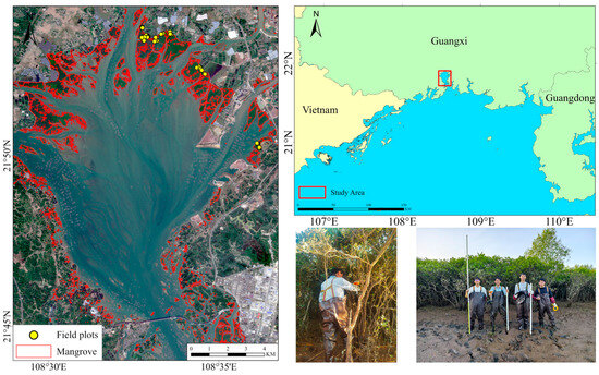
Figure 1.
Study area location, mangrove distribution, and field sampling in the Maowei Sea region.
The Maowei Sea mangrove area, located in the northeastern Beibu Gulf of Guangxi, China, was selected as the study site due to its ecological representativeness, spatial heterogeneity, and significance in regional blue carbon assessment. As one of the largest and most biodiverse estuarine mangrove ecosystems in southern China, Maowei Sea is situated at the transitional zone between tropical and subtropical climates, where complex hydrological dynamics, seasonal tidal regimes, and anthropogenic disturbances converge. In recent years, the Maowei Sea has also become a hotspot for coastal infrastructure expansion, notably serving as the estuarine outlet of the Pinglu Canal—one of China’s major inland waterway projects. This has led to increased land-use pressure, habitat fragmentation, and salinity fluctuations, making it an ideal natural laboratory for testing AGC estimation frameworks under real-world environmental stressors. Given its ecological importance, policy relevance, and representativeness of subtropical Asian mangrove systems, the Maowei Sea offers valuable insights for scalable blue carbon monitoring and coastal management in the context of global change [28,29].
Before conducting the field surveys, we meticulously investigated the distribution ranges of mangrove species, tidal fluctuations, and low-tide timings in the study area. The research team conducted field investigations in the Maowei Sea region from 30 November to 4 December 2024. Survey points were chosen in accessible and safe areas according to the spatial distribution patterns of mangrove species. A total of 40 sample plots were evenly distributed throughout the study area. The dominant species in the study area are primarily S. apetala, K. candel, and A. corniculatum, and these sample plots were mainly located within the communities dominated by these species.
Due to significant variation in mangrove species composition, community succession stages, and plot accessibility, we tailored the size and shape of each sample plot to the characteristics of the respective communities [30]. In areas dominated by S. apetala and K. candel, where the distribution was relatively sparse, sample plots were set at 10 m × 10 m, aligning with the pixel size of Sentinel-2 imagery. Conversely, in areas with denser distributions of A. corniculatum, initial plot size was set at 5 m × 5 m and subsequently adjusted (multiplied by 4) to match the 10 m × 10 m scale of Sentinel data.
Within each sample plot, tree height was measured using a telescopic measuring pole and a handheld laser rangefinder. Meanwhile, the geographic coordinates (latitude and longitude) of each tree, along with the tree species, were recorded using RTK (Real-Time Kinematic) equipment. For S. apetala and K. candel, the diameter at breast height (DBH) was measured at 1.3 m and 0.5 m, respectively. For A. corniculatum, canopy diameter (CD), including the long and short radii of the canopy projection, was measured, assuming the canopy shape to be either circular or elliptical. In the field survey data, S. apetala exhibited relatively high tree heights, with a maximum of 9.1 m and an average of 4.55 m. A. corniculatum showed an average tree height of 2.82 m (range: 1.45–5.6 m) and an average crown width of 1.9 m (range: 0.56–4.36 m). For K. candel, the average tree height was 2.95 m (range: 1.53–5.7 m), and the average DBH was 7.99 (range: 1.9–19.7 cm). The mean tree density was 70 trees per 100 m2, with a range of 17–132 trees per 100 m2. The average AGC density from the field survey was 61.2 Mg C/ha. The maximum AGC density was 200.12 Mg C/ha, and the minimum AGC was 7.74 Mg C/ha.
2.2. Calculation of Mangrove Aboveground Carbon Stocks
Aboveground biomass (AGB) was estimated using species-specific allometric equations. Due to variations in the size, shape, and anatomical structure of mangrove species, as well as differences between the species for which the allometric equations were originally developed, the AGB of many mangrove species is often estimated using generalized allometric equations (Supplementary Table S2). To quantify the AGC stock in mangrove biomass, the AGB was multiplied by a carbon concentration factor. This factor is typically determined through compositional analysis of individual samples, using the dry combustion method (e.g., elemental analyzer). However, due to strict conservation policies in many areas, it is not feasible to fell trees for direct analysis. As such, the AGB of mangroves is commonly converted to carbon by applying a carbon conversion factor, which typically ranges from 0.46 to 0.50. In this study, the carbon concentration ratio for the AGB of mangroves was set at 0.48 [31].
2.3. Remote Sensing Data Collection and Processing
2.3.1. UAV-LiDAR Data
UAV-LiDAR point cloud data were acquired over the sampling area using a LiAir H800 (GreenValley, Beijing, China) laser scanner mounted on a DJI M350 RTK (DJI, Shenzhen, China) Unmanned Aerial Vehicle (UAV). The LiAir H800 operates at a wavelength of 905 nm, features 32 laser channels, and is capable of recording up to 640,000 points per second. The system supports up to 7 returns per pulse, with an estimated laser footprint diameter of approximately 5 cm at the flight altitude of 100 m. Data acquisition was conducted at a flight altitude of 100 m and a flight speed of 10 m/s. To ensure data quality and minimize interference, surveys were performed on 30 November 2024, at 3:00 PM, under clear weather conditions, avoiding persistent winds, and timed during low to mid-tide periods. All LiDAR data processing was conducted using LiDAR360 8.0 (GreenValley, Beijing, China) following a standardized workflow. Initially, noise points were filtered to remove outliers and erroneous returns. The denoised point cloud was subsequently classified into ground and non-ground points using an improved progressive Triangulated Irregular Network (TIN) densification filtering algorithm. Given the relatively flat topography of the mangrove site, the TIN ground filtering algorithm was configured with conservative parameters to enhance ground classification accuracy. Specifically, the maximum iteration angle was set to 6° and the maximum iteration distance to 1.2 m, as recommended for low-relief and vegetated terrain in the LiDAR360 8.0 User Guide. These settings help avoid over-interpolation across non-ground objects such as exposed roots or low-lying vegetation. Accurate ground classification is essential for generating a reliable Digital Elevation Model (DEM), which directly influences the precision of the Canopy Height Model (CHM). By optimizing the TIN parameters, we minimized topographic distortion and ensured that CHM values more accurately reflected true vegetation height. To further improve classification accuracy, ground points were manually reviewed and refined based on visual inspection of cross-sectional profiles, point cloud elevation consistency, and local terrain continuity. Misclassified vegetation or structure points (e.g., low shrubs, roots, or elevated boardwalks) were identified and corrected by referencing intensity values and spatial context. Based on the classified point cloud, a Digital Elevation Model (DEM) was generated from ground points to represent the bare-earth surface. The non-ground points were then normalized using the DEM to remove topographic effects. Subsequently, a Digital Surface Model (DSM) was derived from the normalized non-ground points to capture surface features, including vegetation canopies. To ensure consistency in height calculations, both the DEM and DSM were resampled to a spatial resolution of 10 × 10 m, which corresponds to the CHM grid size and matches the resolution of the satellite imagery. Using consistent resolution between DEM and DSM is critical for minimizing spatial misalignment and ensuring reliable canopy height extraction. The CHM was then calculated using the Raster Calculator tool within LiDAR360 8.0, based on the equation CHM = DSM − DEM, representing vegetation height above the ground surface. All processing steps—including noise filtering, point cloud classification, DEM/DSM generation, and CHM extraction—were completed within a single software environment to ensure methodological consistency and analytical accuracy. All data processing procedures—including noise filtering, ground classification, DEM/DSM generation, and CHM calculation—were conducted in accordance with standard practices outlined in the LiDAR360 User Guide (https://www.lidar360.com/gvi/web/us/file/EN-LiDAR360UserGuide-ZH.pdf) (accessed on 9 January 2025), which provides detailed descriptions of the software tools and parameter settings.
2.3.2. Satellite RS Data
The remote sensing data utilized in this study include Sentinel-2 multispectral imagery, Sentinel-1 C-band synthetic aperture radar (SAR) data, and L-band PALSAR imagery. Given that the sample points were collected during 2024, remote sensing imagery from the same time period in 2024 was selected for analysis to ensure temporal consistency.
Sentinel-2 data were acquired from the Copernicus Open Access Hub (https://dataspace.copernicus.eu/explore-data) (accessed on 1 January 2025), specifically using Level-1C products of the Multispectral Instrument (MSI) from 30 November 2024. The data, provided as Top-of-Atmosphere Reflectance (TOA), were atmospherically corrected using the Sen2Cor processor (version 2.5.5) to produce Bottom-of-Atmosphere Reflectance (BOA) products. To maintain consistency in spatial resolution, the Sen2Res 1.1 plugin developed by the European Space Agency (ESA) was employed to resample all bands to a unified resolution of 10 m. The Sentinel-2 satellite provides 13 spectral bands, including red-edge bands that are particularly sensitive to vegetation characteristics such as mangrove species height, making them ideal for ecosystem monitoring. Moreover, the 5-day revisit cycle of Sentinel-2 enhances the probability of obtaining cloud-free images, which is particularly advantageous for monitoring tropical mangrove areas, often subject to persistent cloud cover [32].
In addition, Sentinel-1 C-band SAR data were used, acquired as part of the “Sentinel-1 SAR GRD” dataset. The data underwent several preprocessing steps, including the application of orbit files, removal of GRD boundary noise, thermal noise reduction, radiometric calibration, and terrain correction (orthorectification), yielding backscatter coefficients (σ°) in decibels (dB). SAR data are notably less sensitive to cloud cover, providing stable and complete imagery for the study area. Dual-polarized (VV + VH) data, from 5 December 2024, were selected for this study, with resampling to a 10 m resolution using the nearest neighbor method to ensure data accuracy.
Finally, PALSAR-2 data were obtained from the Google Earth Engine (GEE) platform. The PALSAR-2 ScanSAR Level 2.2 data had already undergone orthorectification and terrain radiometric correction, ensuring geometric accuracy. The geometric correction process ensured the spatial registration of the PALSAR-2 images, allowing them to align with other remote sensing datasets (e.g., Sentinel-1 and Sentinel-2) within the same coordinate system. This facilitated the accurate fusion of multi-source data. The dual-polarized (HH + HV) data, from 20 November 2024, were selected, and the data were resampled to 10 m using the nearest neighbor method to ensure consistency and suitability for analysis.
To ensure temporal consistency across multi-source datasets, all remote sensing data were selected based on the field sampling date, which was conducted on 30 November 2024. UAV-LiDAR and Sentinel-2 data were acquired on the same day, while PALSAR-2 and Sentinel-1 imagery were selected within a short time window (November 20 and December 5, respectively), thereby minimizing phenological and environmental variations.
For spatial alignment, all datasets—including UAV-LiDAR-derived CHM, Sentinel-1/2, and PALSAR-2 imagery—were reprojected to a unified coordinate system (WGS 84/UTM Zone 49N). Raster matching and alignment were then performed using the “Snap Raster” function in ArcGIS Pro 3.0.2 to ensure strict pixel-to-pixel correspondence among input layers.
To address resolution differences between sensors, all datasets were resampled to a common spatial resolution of 10 m. Bilinear interpolation was applied to continuous variables such as Sentinel-2 spectral reflectance and UAV-LiDAR canopy height, ensuring smooth spatial transitions and reducing pixelation artifacts. For radar backscatter layers from Sentinel-1 and PALSAR-2, nearest neighbor interpolation was used to preserve the physical integrity of the original backscatter values, which are sensitive to interpolation distortion. This tailored resampling strategy, along with consistent temporal and spatial alignment, ensures data compatibility and integrity for subsequent feature extraction and AGC model development. The details of all remote sensing datasets used in this study are summarized in Table 1.

Table 1.
Spectral and textural features used for aboveground carbon (AGC) estimation and their definitions.
3. Methods
The overall workflow of the AGC estimation framework is illustrated in Figure 2.
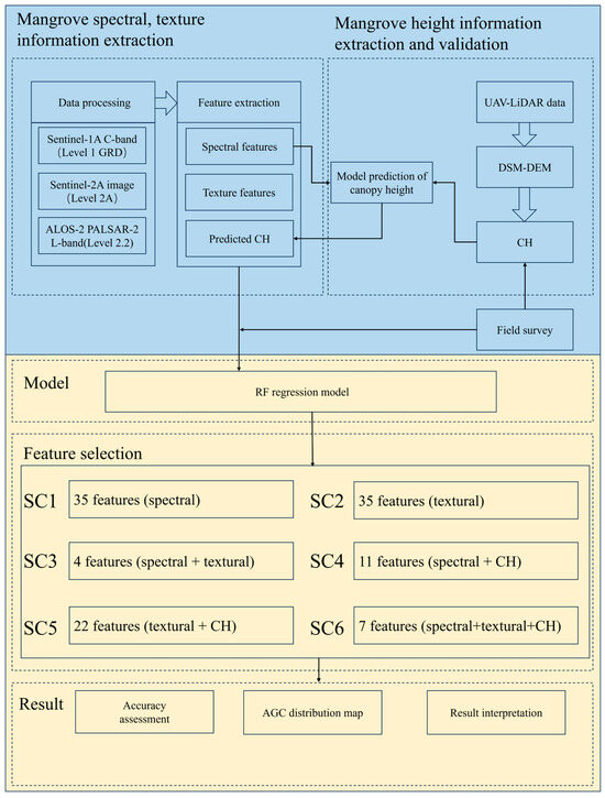
Figure 2.
Workflow of AGC estimation in mangroves using UAV-LiDAR and multi-source satellite data fusion.
3.1. Mangrove Extent Extraction
To delineate the mangrove distribution within the Maowei Sea area, we adopted the Improved Mangrove Mapping Algorithm (IMMA) proposed by Zhao et al. [46], which extracts classification rules from trained RF models to produce transparent and reproducible mangrove maps. This method identifies mangrove extents based on a combination of Sentinel-2-derived spectral indices (e.g., MVI, NDI4, B8/B2) and elevation constraints. The rule set used (e.g., B12 < 0.06 and B8/B2 > 3.50 and elevation < 4.70 and MVI > 2.92 and NDI4 < 0.07) was derived from knowledge distillation of high-accuracy black-box models. The IMMA method achieved an overall accuracy of 82.3% for the coastal region of China and has demonstrated excellent generalization capability and robustness against false positives in complex land cover mosaics. Importantly, the IMMA algorithm has also been shown to mitigate the influence of mixed pixels, particularly in transitional zones such as mangrove–water or mangrove–mudflat boundaries. By utilizing interpretable rule sets and carefully selected spectral ratios (e.g., B8/B2 > 3.5), the IMMA reduces misclassification caused by spectral confusion between mangroves and spectrally similar surrounding land cover types. This advantage has been explicitly demonstrated in the original study, where the IMMA exhibited greater robustness than black-box models in ecologically complex or fragmented coastal areas. Based on this method, we generated a binary mangrove mask at 10 m resolution and subsequently validated and refined the results through visual inspection and reference to high-resolution imagery.
3.2. Extraction of Vegetation Feature
3.2.1. Spectral Feature
To characterize the spectral properties of mangrove canopies, a total of 36 features were extracted, including multispectral reflectance bands and vegetation indices from Sentinel-2 imagery, as well as backscatter coefficients from Sentinel-1 and PALSAR-2 SAR data. Specifically, visible, red-edge, and near-infrared bands (e.g., B2–B8A), along with indices such as the normalized difference vegetation index (NDVI) and Modified Vegetation Index (MVI), were employed to capture information related to chlorophyll content, canopy density, and water stress. Additionally, VV and VH polarizations from Sentinel-1, and HH and HV polarizations from PALSAR-2, were used to infer canopy moisture and structural characteristics [47]. These spectral variables were selected based on their documented relevance to vegetation structure and biomass in mangrove ecosystems, thereby supporting species differentiation, canopy condition assessment, and improved AGC estimation (Table 1).
3.2.2. Textural Feature
To capture spatial heterogeneity within mangrove canopies, textural metrics were calculated from Sentinel-1, Sentinel-2, and PALSAR-2 imagery using the Gray Level Co-occurrence Matrix (GLCM) approach, following standard protocols [48]. These features are particularly valuable in distinguishing structural variation in dense vegetation, where spectral responses may saturate. By encoding canopy roughness, spatial arrangement, and internal texture, GLCM metrics provide complementary structural information that enhances AGC modeling accuracy, especially in mixed-species or structurally diverse mangrove stands (Table 1).
3.2.3. Canopy Height
CH was derived from UAV-based LiDAR data, which provides high-density point clouds for precise vegetation structure characterization. The CH was calculated by subtracting the DEM from the DSM. To ensure the reliability of the LiDAR-derived CH, we validated it using ground measurements (Figure 3). All of the LiDAR point clouds were first tessellated into grids with a cell size of 10 × 10 m, maintaining the same original point as that of the Sentinel-1 and Sentinel-2 imagery. We finally obtained 10,000 candidate LiDAR samples with a size of 10 × 10 m. For enhanced regional CH estimation, we integrated canopy spectral features, dual-polarization synthetic aperture radar (SAR) data (VV and VH polarizations), and employed an RF regression model. This approach follows established methodologies to ensure both the robustness and comparability of CH data for accurate AGC estimation. The performance of the CH model was evaluated with R2 = 0.71 and RMSE = 1.84 m (Supplementary Figure S2), indicating good predictive accuracy. Further details are provided in the Supplementary Materials.
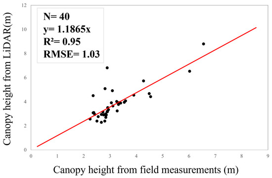
Figure 3.
Comparison of canopy height (CH) from LiDAR and field measurements. The black dots represent individual sample plots, and the red line indicates the fitted linear regression between LiDAR-derived and field-measured canopy height.
3.3. AGC Estimation Model
In this study, AGC estimation was performed using an RF regression model, integrating spectral, textural, and canopy height features derived from Sentinel-1, Sentinel-2, PALSAR-2, and UAV-LiDAR data. The model was trained and optimized using grid search and cross-validation to fine-tune key hyperparameters, ensuring robust performance. Feature importance analysis was conducted to assess the contribution of different variables to AGC prediction (Figure 2).
3.3.1. Feature Selection and Machine Learning Algorithms
The selection of appropriate variables is essential for constructing accurate AGC models. Initial variable selection was based on previous research and domain expertise, with a summary of potentially effective features. However, due to geographical and vegetation differences across study areas, feature selection within a machine learning framework can enhance model efficiency and improve predictive accuracy. In this study, RFE was used for variable selection [49,50]. During the RFE process, an external estimator assigns weights to the features and trains on the initial feature set to assess their importance. The least important feature is removed, and the process is repeated on the pruned set until optimal feature selection is achieved. RF was chosen as the estimator. Feature selection was optimized through cross-validation, and the optimal subset was determined using the coefficient of determination (R2) and root mean square error (RMSE) metrics derived from five-fold cross-validation.
RFE was selected in this study for several reasons. First, it is capable of handling high-dimensional input data and is particularly effective at reducing feature redundancy, which is common in multi-source remote sensing datasets. Second, unlike filter-based or univariate selection methods, RFE considers feature interactions and nonlinear relationships, which are crucial when modeling AGC using spectral, textural, and structural variables. Third, RFE is model-agnostic and integrates well with tree-based learning algorithms such as RF, which provide reliable internal feature importance rankings. These advantages make RFE particularly well suited for identifying robust and compact feature subsets in ensemble-based regression models such as RF.
RF was employed to estimate AGC in mangrove ecosystems. As an ensemble learning method, RF excels in handling high-dimensional datasets and modeling complex relationships between predictor variables [51]. RF has demonstrated strong predictive performance and stability in biomass modeling tasks. The model works by generating multiple decision trees through bootstrap resampling and aggregating their results, which enhances the model’s generalization ability and reduces overfitting. To optimize RF model performance, grid search was used for hyperparameter tuning. This method explores a predefined range of hyperparameters and evaluates different combinations using cross-validation, ensuring that the optimal parameter set is selected. This process improves the model’s predictive accuracy and its ability to reliably estimate AGC in mangroves.
3.3.2. Accuracy Assessment
In this study, all 40 samples were randomly divided into a training set (80%) and a testing set (20%) and applied to the RF model. Although the overall sample size is relatively small, this 80/20 partition strategy is widely adopted in mangrove carbon estimation studies [24,52,53]. To further mitigate the limitations associated with a small testing set, a five-fold cross-validation (CV) approach was employed during the training process to optimize the model’s hyperparameters and assess generalization performance. This strategy ensures that each sample is used for both training and validation across multiple iterations, thereby enhancing the robustness of model evaluation and minimizing overfitting risk. As noted by Pedregosa et al. [54], cross-validation is an essential tool in small-sample scenarios, offering reliable performance estimation by generating multiple train/test splits from limited data. The Scikit-Learn library was utilized to fine-tune the optimal parameters of the machine learning model. Model performance was assessed using the coefficient of determination (R2) and RMSE metrics to compare the effectiveness of different feature combinations. The R2 metric evaluates how well the model’s predictions fit the observed values, while RMSE quantifies the prediction error. The consistent improvements observed across various feature combinations further support the validity and stability of the evaluation results despite the relatively small testing set.
where and represent the observed values and the mean of the AGC, respectively, while denotes the predicted values. To further analyze the impact of different vegetation feature combinations and machine learning approaches on the estimation of AGC, we computed the average R2 values for different feature subsets. All analyses were conducted using Python software (version 3.9).
4. Results
4.1. Modeling Results Comparison Between Different Features
In this research, features were screened using RFE, and five-fold cross-validation was employed to evaluate the accuracy of different data combinations. The features used are derived from three types of data: spectral features, textural features, and canopy height. The estimation capabilities of the three types of data and the changes in model accuracy before and after performing RFE were assessed separately by performing AGC estimation with single or multiple data combinations. The results are summarized in Table 2 and illustrated by scatterplots in Figure 4.
Table 2.
Test results for various feature combinations and their number of features calculated based on Recursive Feature Elimination (RFE) feature selection.
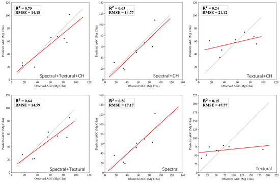
Figure 4.
Comparison of AGC prediction models using different combinations of predictor variables. The black dots represent the testing samples, the red line indicates the fitted regression line between predicted and observed AGC, and the dotted line represents the 1:1 reference line.
Among all tested feature combinations, the integration of spectral and textural features yielded notable improvements in model performance compared to individual sources. For instance, the spectral + textural model achieved an R2 of 0.64 and an RMSE of 14.59 Mg/ha after RFE, outperforming the use of spectral features alone (R2 = 0.50, RMSE = 17.17 Mg/ha) or textural features alone (R2 = 0.15, RMSE = 47.77 Mg/ha). This suggests that incorporating spatial variability through texture metrics enhances the sensitivity of spectral-based models to vegetation structure. While the improvement from spectral to spectral + CH in terms of R2 (from 0.50 to 0.63) might appear moderate, the RMSE significantly decreased from 17.17 to 14.77 Mg/ha, clearly indicating a meaningful enhancement in prediction accuracy. Moreover, this model required fewer features (11 features) after RFE, improving model simplicity and generalization. The addition of CH led to further substantial improvements. The model integrating spectral, textural, and CH features achieved the best performance (R2 = 0.75, RMSE = 14.18 Mg/ha) with only seven RFE-selected features. This indicates that CH, as a structural variable directly related to vertical biomass distribution, plays a dominant role in improving AGC prediction. Notably, even though texture or CH alone contributed limitedly when used in isolation (e.g., CH + texture yielded R2 = 0.24), their synergistic effect with spectral data significantly enhanced model accuracy. Figure 4 provides a visual comparison of predicted vs. observed AGC values across different feature combinations. Models incorporating CH demonstrated a closer alignment with the 1:1 reference line, smaller dispersion, and notably lower prediction errors, further confirming the robustness and reliability of CH as a critical variable.
In summary, these results underscore the crucial role of structural metrics, especially canopy height, in addressing signal saturation issues in high-biomass mangrove forests. The integration of spectral, textural, and structural features provides a more comprehensive depiction of canopy heterogeneity, enabling improved AGC estimation and greater generalization capability across spatially diverse regions.
4.2. Mangrove AGC Map of Maowei Sea
The total AGC of the Maowei Sea mangroves is estimated at 88,363.73 metric tons, with a mean AGC density of 53.01 Mg C/ha (Figure 5). Spatial distribution analysis reveals that higher AGC values are concentrated in the northwestern coastal zones, particularly in Kangxiling and Tuanhe Island, where mature, planted S. apetala stands with well-developed canopy structures dominate, contributing significantly to the carbon stock. In contrast, the S. apetala communities in the northwestern part of Jianxinwei have mainly been established through natural regeneration from propagules dispersed by tidal currents from Kangxiling. These younger and more sparsely distributed stands exhibit relatively lower AGC. Meanwhile, the eastern part of Jianxinwei is primarily occupied by mature A. corniculatum communities, interspersed with scattered K. candel, resulting in higher AGC values due to well-structured canopy layers and substantial biomass accumulation. Compared to existing regional or global AGC datasets derived from moderate-resolution satellite imagery (e.g., 30 m or coarser), our final AGC map offers improved spatial detail (10 m resolution) and enhanced structural sensitivity by incorporating UAV-LiDAR-derived canopy height. This fine-scale mapping allows better identification of intra-patch variability and supports localized ecosystem management and impact assessment.
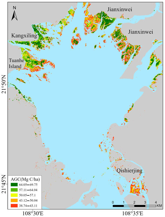
Figure 5.
Mangrove AGC map of Maowei Sea.
5. Discussion
5.1. Contribution of Canopy Height from UAV-LiDAR to Multi-Source AGC Modeling in Mangroves
Optical and SAR remote sensing have been widely applied in forest biomass estimation, but both suffer from signal saturation effects in high-biomass regions due to their inherent physical limitations. Optical sensors (e.g., Landsat and Sentinel-2) estimate biomass through empirical relationships between spectral reflectance and vegetation indices such as the NDVI. However, in dense canopy forests where the crown is fully closed, the reflectance signal becomes saturated, weakening its responsiveness to variations in canopy structure [55]. Similarly, SAR sensors (e.g., Sentinel-1 and ALOS PALSAR) use backscatter intensity to estimate biomass but are constrained by limited penetration capabilities: the C-band saturates around 50–80 Mg/ha and the L-band around 100–150 Mg/ha, failing to resolve structural complexity in high-biomass stands [56]. Although texture features derived from GLCM, such as contrast and entropy, can partially compensate for spectral and radar limitations—especially in low-to-moderate biomass forests—their sensitivity also diminishes in highly homogeneous closed canopies [57,58]. As such, biomass estimation methods that rely solely on spectral or SAR data often encounter accuracy bottlenecks in mangrove ecosystems with high biomass density.
To address these limitations, recent studies have incorporated structural parameters—especially canopy height—to enhance model responsiveness to biomass variation. Satellite LiDAR systems such as GEDI have made it possible to acquire canopy height measurements at global scales for AGC estimation. For instance, Zhao et al. integrated GEDI-derived canopy height with Sentinel-2 spectral features to estimate urban biomass, achieving an R2 of 0.58 and RMSE of 14.25 Mg/ha [59]; Tian et al. reported improved accuracy (R2 = 0.75, RMSE = 17.34 Mg/ha) in a similar fusion framework over forested regions in Fujian, China [60]. However, GEDI’s spatial sampling is limited by its orbital characteristics: with a footprint diameter of ~25 m and inter-track spacing exceeding 600 m, GEDI provides discrete observations that are insufficient to capture the structural heterogeneity of mangrove forests. In areas with rapid structural variation or mixed-species assemblages, the performance of GEDI-based estimation can be suboptimal. Furthermore, in forests with canopy heights exceeding 20 m, multiple scattering effects and attenuated ground returns can introduce uncertainty in height retrieval [15,61]. In contrast, UAV-based remote sensing offers centimeter-level spatial resolution and can capture fine-scale canopy structure and height variation. In the Maowei Sea region, Tian et al. achieved an AGB estimation accuracy of R2 = 0.83 (RMSE = 22.76 Mg/ha) by integrating UAV-derived spectral, structural, and texture features [24]. Dhakal et al. reported even higher accuracy in agricultural applications (R2 = 0.93, RMSE% = 15.97%) [62]. UAV-LiDAR generates dense point clouds capable of accurately delineating both terrain and canopy heights, thereby complementing the limitations of spectral and SAR data in densely vegetated environments. Nevertheless, due to limited flight efficiency and coverage, UAV approaches alone are insufficient for large-scale carbon stock mapping.
To achieve both high estimation accuracy and spatial generalization, this study integrates UAV-LiDAR-derived CH with multi-source satellite data (Sentinel-1, Sentinel-2, and ALOS PALSAR-2) for regional-scale modeling of AGC in the Maowei Sea mangrove ecosystem. Unlike conventional upscaling frameworks that propagate AGB estimates sequentially from field plots to UAV data and subsequently to satellite imagery [63,64], this study adopts a structure-oriented approach. High-resolution CH data obtained from UAV-LiDAR in representative subregions are fused with spectral features to establish predictive models, enabling the interpolation of canopy height across the broader mangrove landscape.
Rather than transferring biomass estimates across scales, our framework leverages canopy height—a physiologically meaningful and directly observable structural variable—as the core modeling input (Figure 6). CH was a key structural parameter in allometric equations—the model maintains sensitivity to biomass variation even in high-biomass mangrove stands, thus mitigating the saturation effects commonly observed in NDVI-based optical methods and polarization backscatter coefficients. By incorporating CH, the model maintains sensitivity to vertical structural variation, which is often lost in traditional reflectance- or backscatter-driven approaches. The contribution of UAV-derived CH is threefold: (1) it remains responsive in optically saturated or SAR-penetration-limited zones; (2) it bridges the scale gap between ground plots and coarse-resolution satellite data; and (3) it enhances model robustness across heterogeneous canopy conditions.
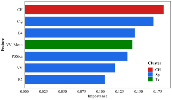
Figure 6.
Feature importance for AGC estimation in mangroves.
Our fusion-based model achieved an R2 of 0.75 and RMSE of 14.18 Mg/ha, outperforming satellite-only approaches, such as the approach of Pham et al., who reported R2 = 0.63 and RMSE = 25.08 Mg/ha. While prior studies integrating UAV and satellite data [63,64] (Niu et al., 2024: R2 = 0.74; Wang et al., 2019: R2 = 0.67) demonstrated improved accuracy, they relied on multi-level AGB regression, which may introduce cumulative uncertainty. In contrast, our approach reduces such error propagation by directly modeling canopy structure rather than AGB, thus improving generalizability and resilience to ecological heterogeneity. Table 3 summarizes the performance and scale applicability of three typical modeling strategies: (1) satellite-only models (R2 = 0.58–0.75), (2) UAV-only approaches with high local accuracy (R2 up to 0.93) but limited spatial extent, and (3) UAV–satellite fusion methods, which offer an effective compromise between accuracy and scalability. These results underscore the advantages of structure-driven, cross-scale modeling for reliable estimation of AGC in mangrove ecosystems.
Table 3.
Comparison of sensor types in terms of accuracy and spatial scale for estimating aboveground biomass across vegetation types.
The differences in model accuracy across studies can be attributed to several key factors. First, satellite-only models often suffer from signal saturation in dense mangrove canopies due to limited sensitivity of spectral indices and radar backscatter at high biomass levels, particularly in monospectral NDVI-based approaches or C-band SAR applications. Second, while UAV-only methods yield high local accuracy, they are constrained by limited spatial coverage and lack of regional generalizability. Third, many UAV–satellite fusion studies adopt hierarchical regression frameworks that estimate AGB in stages (e.g., field-to-UAV and UAV-to-satellite), which can compound uncertainty at each step due to error propagation and scaling mismatch.
In contrast, our structure-oriented modeling approach directly integrates UAV-derived CH into satellite-scale models, using canopy height as a physiologically grounded proxy that is less prone to saturation and more robust to interspecies variation. This allows for continuous, spatially coherent AGC estimation across structurally heterogeneous mangrove landscapes. Moreover, the use of RFE for feature selection minimizes collinearity and redundancy, further enhancing model robustness compared to conventional fusion frameworks. These methodological distinctions help explain the improved performance of our model (R2 = 0.75, RMSE = 14.18 Mg/ha) relative to existing approaches.
While the proposed UAV–satellite fusion framework demonstrates strong performance at the regional scale, its scalability to national or continental levels requires further consideration, particularly in light of the limited spatial coverage of UAV platforms. One promising pathway is to use UAV-LiDAR as a source of calibration data to support the training and validation of large-scale models built upon wall-to-wall satellite observations. In this context, UAV-derived canopy height samples collected from representative ecological zones can serve as structural references for extrapolating forest metrics across broader extents. This concept has been increasingly recognized in recent studies, where UAV or airborne LiDAR data are used to calibrate or guide satellite-based forest structure modeling. For example, Jian et al. demonstrated that UAV-LiDAR data could effectively calibrate stereo optical satellite imagery (ZY-3) for accurate canopy height estimation, underscoring the value of UAV data as local reference sources in large-scale applications [65]. Similarly, Wang et al. integrated airborne LiDAR and GEDI waveform data to calibrate large-area canopy height models using Sentinel-2 spectral features [66]. In a national-scale application, Li et al. utilized airborne LiDAR-derived canopy height data from the Japan Forestry Agency, in combination with multi-source satellite inputs (Sentinel-2, ALOS-2 PALSAR, and SRTM), to train RF models and generate a 10 m resolution canopy height map across Japan [67]. These studies collectively highlight how high-resolution structural references, even if spatially sparse, can be effectively leveraged to enable scalable and accurate forest structure estimation. With the growing availability of high-quality satellite and airborne datasets, such hybrid frameworks offer a promising foundation for extending AGC monitoring to national or even continental scales in mangrove and other forest ecosystems.
Nevertheless, the broader application of this UAV–satellite fusion framework is subject to several spatial, logistical, and economic constraints. First, the spatial applicability of the current model is primarily limited to coastal mangrove zones with relatively similar species composition, canopy structures, and tidal regimes as the training region (e.g., Maoweihai in Guangxi). Extrapolating the model to ecologically distinct mangrove systems—such as those in tropical Southeast Asia or arid coastal regions—may require re-calibration or re-training with locally representative data. Second, UAV-LiDAR campaigns, though cost-effective at small scales, remain logistically demanding and expensive for large-scale deployment, especially in remote or protected areas where flight permissions are restricted. The acquisition cost and time investment for UAV-based canopy height mapping may pose practical barriers to widespread adoption. Furthermore, harmonizing datasets from different satellite sensors and UAV platforms across seasons introduces additional technical complexity. Therefore, while the proposed framework is promising in regional applications and scalable with proper calibration, its broader implementation necessitates careful consideration of ecological representativeness, cost-efficiency, and data integration feasibility. Future work could explore semi-automated UAV data acquisition pipelines, cross-region transfer learning, and integration of sensors (e.g., LiDAR-equipped satellites) to further reduce these bottlenecks and enhance model generalizability.
5.2. Contributions of Multidimensional Features to Mangrove AGC Estimation and Implications of Feature Selection
While CH plays a dominant role in AGC estimation, spectral and textural features remain indispensable for capturing complementary information on vegetation composition, physiological status, and surface structure—particularly under species-specific ecological conditions. As shown in the feature importance analysis (Figure 6), several spectral indices and texture metrics make non-negligible contributions to AGC prediction when used in conjunction with CH, offering a multidimensional representation of mangrove canopy properties. However, the predictive influence of these features varies with canopy density, species-specific traits, and structural heterogeneity.
In this study, the B4 band, B2band, and VV band have relatively small direct impacts on mangrove carbon stock and generally exhibit negative correlations (Figure 7). The B4 primarily reflects vegetation’s photosynthetic activity, and its reflectance is closely related to chlorophyll content [68]. Healthy vegetation typically absorbs more red light, while vegetation in poorer health reflects more red light, resulting in lower carbon stock. Therefore, this band shows a negative correlation with carbon stock. The B2 band, located in the blue region of the visible spectrum, is strongly affected by chlorophyll absorption and atmospheric or surface water scattering, which limits its reliability in vegetated and coastal environments [69]. In mangrove ecosystems, the combination of intensified specular reflection from tidal waters and high chlorophyll absorption further attenuates blue reflectance, limiting the utility of B2 in estimating AGC, contributing less to AGC estimation, and negatively correlating with AGC (Figure 6). The VV band from SAR data captures canopy density and surface roughness, offering useful structural insights for AGC estimation. However, its limited penetration capability in high-biomass forests results in saturation effects, reducing its standalone predictive power. Despite this, VV-based features remain valuable when integrated with spectral and canopy height metrics, contributing to improved AGC modeling under multi-source data frameworks [70]. In low-density mangrove forests, radar wave reflectance is typically enhanced, thus showing a negative correlation with carbon stock. However, despite the small contribution of these bands to carbon stock estimation individually, they still provide supplementary information in the fusion of multi-source data [71], particularly within different mangrove species’ growth environments (Figure 7). This indicates that, although spectral and radar bands contribute limitedly in certain environments, under specific ecological conditions, they remain valuable in enhancing the reliability of carbon stock estimation.
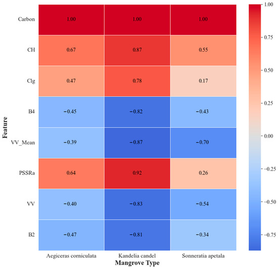
Figure 7.
Correlation between features and mangrove types for AGC.
As shown in Figure 7, different mangrove species exhibit distinct correlation patterns with key predictive features, indicating species-specific sensitivities in AGC estimation. For instance, K. candel shows strong positive correlations with CH (0.87), Clg (0.78), and PSSRa (0.92), highlighting the effectiveness of canopy height and chlorophyll-related indices for this species. In contrast, S. apetala demonstrates a weak positive correlation with Clg (0.17) but a strong negative correlation with VV_Mean (–0.70), suggesting that increased radar texture variability corresponds to lower AGC in dense, structurally uniform stands. This may reflect signal saturation and reduced canopy heterogeneity in S. apetala-dominated areas, limiting the utility of conventional spectral and textural features. In monoculture zones where a single species dominates, the discriminative capacity of texture-based metrics (e.g., CMV and CMSM) is likely reduced due to the lack of inter-species structural variability. Previous studies have shown that texture features are more effective in mixed-species mangrove stands with varying leaf morphology and branching complexity [72]. Therefore, species homogeneity may constrain the effectiveness of textural features, underscoring the importance of integrating structural and physiological indicators in AGC modeling for such environments.
Previous studies have typically employed extensive sets of multi-source features—including spectral, textural, and structural parameters—to maximize the predictive potential for estimating mangrove AGC [25,73]. However, these studies consistently encountered significant redundancy due to high collinearity among selected variables, limiting the effective utilization of the information embedded within these datasets. Consequently, only a small subset of features genuinely contributed to accurate AGC estimation, with many others offering minimal incremental value. In contrast, our study systematically addressed this limitation by employing RFE to rigorously evaluate and reduce redundancy among multi-source variables. This methodological refinement effectively identified a concise yet powerful subset of predictors that substantially improved both accuracy and interpretability of the AGC estimation model. Notably, the inclusion of UAV-derived CH emerged as a critical structural predictor, markedly enhancing model performance and demonstrating that carefully selected, structurally representative variables significantly outperform more extensive but redundant feature sets. Therefore, our findings emphasize that strategic selection and integration of complementary and structurally meaningful predictors, particularly canopy height, are essential for constructing robust, reliable, and parsimonious AGC estimation models in mangrove ecosystems.
Note: CH = canopy height; Clg = canopy leaf greenness index; B4, B2 = Sentinel-2 bands (Red and Blue); VV_Mean = Texture feature (GLCM mean) from Sentinel-1 VV polarization; PSSRa = Pigment Specific Simple Ratio; VV = Sentinel-1 VV polarization backscatter; see Table 1 for full definitions and formulas.
5.3. Comparison of Mangrove Height and AGB in Maowei Sea and Other Regions
The comparison of mangrove structural characteristics across different regions reveals significant spatial variability in canopy height and AGB. In China, mangrove vegetation exhibits a clear latitudinal gradient. For instance, in subtropical zones such as the Zhangjiang Estuary in Fujian (~24° N), mangroves are typically stunted, with an average height of only ~3.1 m and AGB values ranging between 80 and 90 Mg/ha [74,75]. In contrast, warmer southern areas such as the Maowei Sea in Guangxi and Hainan Island (~18–20° N) support taller mangroves with mean heights of 6–7 m and AGB values exceeding 100 Mg/ha [64]. Specifically, the mangroves in Hainan exhibit an average canopy height of 6.99 m and an AGB of 128 Mg/ha, significantly higher than those in other Chinese provinces. For example, the average AGB in the Jiulong River Estuary, Fujian, is ~79 Mg/ha [75] and ~55 Mg/ha in Shenzhen Bay, Guangdong [76], both markedly lower than the values observed in Hainan. These regional differences demonstrate that, even within a relatively narrow latitudinal range, varying ecological conditions can lead to significant differences in mangrove structure and carbon storage capacity.
Regional differences in mangrove canopy height and AGB are driven by multiple factors, among which latitude and climate are primary determinants. It is well established that mangrove height generally decreases with increasing latitude—a global pattern whereby the tallest mangrove stands are found in equatorial regions, while subtropical mangroves tend to be shorter [77]. In China, mangroves are primarily located near the tropical–subtropical transition zone (~18–28° N). In regions such as Fujian and Guangdong, colder winter temperatures and occasional frost events can inhibit mangrove growth. In contrast, the tropical climate of Hainan—with year-round warmth and a prolonged growing season—provides more favorable conditions for mangrove development [78].
Species composition is another critical factor affecting mangrove structure and carbon storage potential. In tropical southern China, particularly in Hainan and parts of Guangxi, mangrove communities contain large-canopy species such as Bruguiera sexangula and S. apetala, which often exceed 8 m in height and exhibit high biomass accumulation potential. These species are key contributors to the higher canopy height and AGB observed in Hainan. In the present study area, the Maowei Sea, S. apetala is also a dominant species, widely distributed in Kangxiling Town and surrounding zones, and exhibits relatively high canopy structure and biomass. Conversely, in higher-latitude subtropical regions such as Fujian and Guangdong, mangrove communities are typically dominated by cold-tolerant, low-stature species, including K candel, Avicennia marina, and A. corniculatum, with typical heights ranging from 2 to 4 m [79]. This compositional limitation directly constrains the maximum attainable canopy height and AGB in high-latitude mangrove ecosystems, thereby contributing to the observed discrepancies in carbon stock estimates across regions [64].
Beyond biogeography, hydrothermal conditions and geomorphological settings also play essential roles in mangrove development. River deltas and regions with high rainfall provide ample freshwater and nutrients, enhancing mangrove productivity [80]. Freshwater input effectively mitigates salinity stress and promotes canopy development and is regarded as a critical factor in vertical structural formation [81]. In contrast, arid or hypersaline environments restrict growth and often result in low-stature shrub-like mangrove communities with reduced productivity. For example, in the semi-arid coastal zone of northwestern Australia (~22° S), the average mangrove height is only ~3 m, with AGB levels around 70 Mg/ha—conditions largely attributed to the region’s harsh, dry climate [82,83].
To further contextualize China’s mangrove forests at a global scale, we compared average canopy height and AGB values across representative regions (Table 4). Results indicate that the Maowei Sea mangroves (mean height ~6.08 m, AGB ~108 Mg/ha) outperform higher-latitude counterparts such as Florida, USA (~25° N, ~5 m height, AGB 30–40 Mg/ha) [84] and northwestern Australia (~22° S, ~3 m height, AGB ~70 Mg/ha) [83]. However, these values remain lower than those of equatorial tropical mangroves, such as those in coastal Africa (mean height ~7.5 m, AGB ~116 Mg/ha) [85] and Papua, Indonesia, where average tree height reaches ~21 m and AGB density climbs to 293 Mg/ha [86]. These exceptionally high-biomass mangrove stands, found in humid tropical estuaries with abundant freshwater and nutrient supply, represent some of the tallest and most carbon-rich mangroves globally.
Table 4.
Comparison of tree height and aboveground biomass (AGB) of mangroves in different regions.
These findings underscore the necessity of mapping mangrove canopy height and AGB distributions at large spatial scales. Traditional mangrove maps typically focus only on spatial extent and fail to capture structural variation. For instance, two mangrove areas of equal size may differ significantly in ecosystem functioning: one being a tall, mature forest and the other a low-stature shrubland. Taller mangrove stands generally store more AGC and provide more complex vertical habitat structures that support greater biodiversity. Therefore, generating high-resolution maps of mangrove canopy height and AGB is essential for precise carbon accounting, identifying blue carbon conservation hotspots, and guiding restoration and sustainable management strategies.
5.4. Method Uncertainty Considerations and Future Perspectives
The estimation of AGC in mangrove ecosystems using multi-source remote sensing and field data is inherently affected by various sources of uncertainty. These uncertainties originate primarily from (1) remote sensing data acquisition and processing, (2) field measurement quality, and (3) statistical modeling procedures. First, multi-source satellite data—such as Sentinel-1, Sentinel-2, and PALSAR-2—possess intrinsic differences in sensor characteristics (e.g., spectral bandwidth, polarization, and incidence angle) and spatial resolutions. Additionally, the preprocessing procedures involved, including radiometric calibration, geometric registration, and atmospheric correction, may introduce systematic or random errors. These inconsistencies could affect the comparability and accuracy of extracted features, thereby propagating error into the AGC estimation model. Second, the 10 m spatial resolution used in this study, though widely adopted in mangrove mapping, may not sufficiently resolve fine-scale canopy heterogeneity. In particular, at mangrove fringe zones or tidal creek edges, the presence of mixed pixels containing water, mudflats, and vegetation complicates spectral signal interpretation. Seasonal changes in vegetation phenology and water level dynamics further increase the spectral variability, introducing temporal uncertainty in reflectance-based indicators. Third, field measurements of canopy height, canopy diameter, and diameter at breast height—used to calibrate and validate AGC models—are subject to observer bias, instrumental limitations, and ecological constraints. In dense mangrove stands, difficult terrain and high vegetation density often prevent accurate and consistent measurements. Errors in DBH and height can be significantly amplified when propagated through nonlinear allometric equations, resulting in biased AGC estimations. In addition, species misidentification or geolocation errors during field surveys may also introduce noise in the ground truth dataset. Finally, the machine learning algorithm itself (RF, in this case) is another source of uncertainty. Model performance can be influenced by sample representativeness, overfitting or underfitting due to hyperparameter settings, and randomness in feature selection during model training. These factors may limit model generalizability, particularly when applied beyond the original sampling zones.
To address the above-mentioned sources of uncertainty, future research should pursue targeted strategies to improve model generalizability, robustness, and ecological interpretability. First, to mitigate the impact of sensor inconsistencies and preprocessing errors across multi-source satellite data (e.g., Sentinel-1/2, PALSAR-2), future studies could explore the use of sensor-specific correction models, radiometric normalization techniques, or cross-sensor feature harmonization frameworks. Additionally, the incorporation of physics-informed machine learning approaches—such as Physics-Informed Neural Networks (PINNs)—can help reduce the reliance on empirically extracted features by embedding ecological principles (e.g., allometric equations) into model structure, thereby improving consistency across sensors and time periods [87,88]. Second, to compensate for spatial resolution limitations and mixed-pixel effects, particularly in fringe zones and tidal interfaces, future work could integrate higher-resolution satellite data sources (e.g., GF-2, Pléiades Neo, and WorldView) as reference layers for downscaling or super-resolution learning, particularly when combined with UAV-LiDAR-derived structural features. Time-series modeling may also help capture phenological dynamics and tidal fluctuations, reducing temporal uncertainty in reflectance-based indicators. Such spatiotemporal integration is especially valuable in environments characterized by seasonal or sub-daily variability. Third, to reduce field-based measurement error and ecological sampling bias, future research should adhere strictly to standardized forest inventory protocols and invest in enhanced training for field personnel. Expanding the number and spatial representativeness of ground plots—particularly in structurally complex or difficult-to-access zones—and increasing their temporal sampling frequency (e.g., seasonal or annual remeasurements) can improve ground-truth data quality and support the detection of AGC dynamics over time. In parallel, efforts should be made to minimize species misidentification and geolocation inaccuracies, including the use of GPS post-correction, botanical verification, and digital field mapping systems. To further enhance the ecological interpretability and accuracy of AGC estimation, future work will consider incorporating additional biometric variables. Tree age can serve as an indicator of stand development and long-term growth dynamics, while wood density is a key factor influencing carbon accumulation, especially among trees with similar canopy height. Integrating these complementary parameters may help reduce residual uncertainty and improve model performance across heterogeneous mangrove structures. Finally, to address uncertainty stemming from the modeling process itself, future work should implement formal sensitivity analysis (e.g., Sobol or variance decomposition methods) to quantify the influence of input variables such as CH, VV_Mean, or Clg. Such analysis can guide feature selection, reduce redundancy, and improve model parsimony [89,90,91]. Additionally, incorporating ancillary non-remote sensing variables—such as soil salinity, elevation, organic matter content, or local climate (e.g., rainfall and temperature)—may significantly enhance model performance by capturing ecological gradients not observable from spectral or structural data alone. These improvements can collectively enhance model applicability across different mangrove types and biogeographic contexts.
Looking ahead, several additional research avenues warrant further exploration to enhance the ecological interpretability of AGC estimation in mangrove ecosystems. First, the coupling between aboveground and belowground carbon pools remains insufficiently understood. While this study focused on AGC, future field campaigns will incorporate soil organic carbon (SOC) sampling and spatial analysis to investigate its correlation with UAV-derived canopy metrics, aiming to uncover structural linkages between aboveground and belowground carbon stocks.
Second, although CH was employed as the primary structural parameter in this study due to its stability and transferability, the high-density UAV-LiDAR point clouds collected provide a valuable opportunity to derive more detailed three-dimensional canopy metrics—such as porosity, clumping index, and foliage distribution. These structural attributes are known to modulate light interception and photosynthetic light use efficiency (LUE), particularly in complex mangrove canopies. Future localized analyses will explore these metrics to improve the mechanistic understanding of canopy structure–function interactions.
Finally, the explicit inclusion of photosynthetically active radiation (PAR) in AGC modeling represents a promising direction. While PAR was not incorporated in the current study due to the lack of co-temporal in situ observations and the coarse spatial resolution of existing satellite products, several spectral variables used—such as Sentinel-2 red-edge bands and the canopy leaf greenness index—are physiologically linked to chlorophyll content and light absorption and thus may serve as indirect indicators of LUE. Future efforts will consider integrating modeled or measured PAR datasets (e.g., from GLASS, MODIS, or ground-based quantum sensors) with UAV-derived structural traits to more accurately characterize LUE and its influence on AGC variation across heterogeneous mangrove landscapes.
6. Conclusions
This study demonstrates the effectiveness of integrating UAV-derived LiDAR with multi-source satellite imagery (Sentinel-1, Sentinel-2, and PALSAR-2) for accurate estimation of mangrove CH and AGC. Canopy height emerged as a key structural feature that mitigates spectral saturation and significantly improves AGC model performance. The fusion of spectral, textural, and structural variables yielded optimal results (R2 = 0.75, RMSE = 14.18 Mg C/ha), confirming the value of multi-dimensional feature integration. While previous studies have advanced satellite-based carbon mapping through machine learning or multi-temporal fusion, they are often limited in retrieving fine-scale structural indicators such as CH. UAV-based LiDAR offers precise vertical structure information that bridges this resolution gap, making it a critical complement to satellite observations. The Maowei Sea mangroves exhibited a mean canopy height of 6.08 m and an average AGC density of 53.01 Mg C/ha, with a total regional AGC stock of 88,363.73 Mg. These findings underscore the potential of UAV–satellite fusion frameworks for scalable, accurate blue carbon monitoring in structurally complex ecosystems. The methodology presented here contributes to improving regional carbon accounting and supports climate mitigation, coastal ecosystem resilience, and the sustainable management of blue carbon resources in the context of global environmental change.
Supplementary Materials
The following supporting information can be downloaded at: https://www.mdpi.com/article/10.3390/su17188211/s1, Figure S1: Mangrove CH map of Maowei Sea; Figure S2: Scatterplot of predicted vs. observed CH from the RF model; Figure S3: Feature importance for CH prediction in the RF model; Table S1: Mangrove plot characteristics (data are presented as mean); Table S2: Allometric growth equations of different mangrove communities; Table S3: Indicators for predicting CH based on random forest (RF). References [92,93,94] has been cited to in the supplementary material.
Author Contributions
Conceptualization, methodology, software, validation, X.M. and Q.L.; formal analysis, X.M., W.X. and Q.L.; investigation, W.X., X.M., W.W. (Wenqian Wu), S.D. and W.W. (Wenhuan Wang); data curation, X.M., S.D. and W.X.; writing—original draft preparation, X.M.; writing—review and editing, W.Z. and Y.W.; visualization, S.D., W.W. (Wenqian Wu) and W.W. (Wenhuan Wang); supervision, W.Z. and Y.W.; funding acquisition, Y.W. All authors have read and agreed to the published version of the manuscript.
Funding
This research was funded by the Guangxi Science and Technology Major Program, grant number GUIKEAA23062054; the Science and Technology Research and Development Projects of Guangxi Institute of Industrial Technology, grant number CYY-HT2023-JSJJ-0037; and the Guangxi Key Research and Development Program, grant number GUIKEAB24010248.
Institutional Review Board Statement
Not applicable.
Informed Consent Statement
Not applicable.
Data Availability Statement
The data presented in this study are available on request from the corresponding author.
Conflicts of Interest
The authors declare no conflicts of interest.
Abbreviations
The following abbreviations are used in this manuscript:
| Abbreviation | Full Term |
| AGC | Aboveground Carbon |
| AGB | Aboveground Biomass |
| GEE | Google Earth Engine |
| GLCM | Gray Level Co-occurrence Matrix |
| DEM | Digital Elevation Model |
| DSM | Digital Surface Model |
| RF | Random Forest |
| RFE | Recursive Feature Elimination |
| R2 | Coefficient of determination |
| RMSE | Root mean square error |
| CH | Canopy Height |
| UAV | Unmanned Aerial Vehicle |
| LiDAR | Light Detection and Ranging |
| RTK | Real-Time Kinematic |
| TIN | Triangulated Irregular Network |
| SAR | Synthetic Aperture Radar |
| GEDI | Global Ecosystem Dynamics Investigation |
| ICESat-2 | Ice, Cloud, and Land Elevation Satellite-2 |
References
- Donato, D.C.; Kauffman, J.B.; Murdiyarso, D.; Kurnianto, S.; Stidham, M.; Kanninen, M. Mangroves among the most carbon-rich forests in the tropics. Nat. Geosci. 2011, 4, 293–297. [Google Scholar] [CrossRef]
- Atwood, T.B.; Connolly, R.M.; Almahasheer, H.; Carnell, P.E.; Duarte, C.M.; Lewis, C.J.E.; Irigoien, X.; Kelleway, J.J.; Lavery, P.S.; Macreadie, P.I.; et al. Global patterns in mangrove soil carbon stocks and losses. Nat. Clim. Change 2017, 7, 523–528. [Google Scholar] [CrossRef]
- Campbell, A.D.; Fatoyinbo, T.; Charles, S.P.; Bourgeau-Chavez, L.L.; Goes, J.; Gomes, H.; Halabisky, M.; Holmquist, J.; Lohrenz, S.; Mitchell, C.; et al. A review of carbon monitoring in wet carbon systems using remote sensing. Environ. Res. Lett. 2022, 17, 25009. [Google Scholar] [CrossRef]
- Yi, X.; Jie, L.; Shengfa, Y.; Wenjie, L. Impact of channel deepening on the saltwater intrusion process in the Qinjiang River estuary, Southeast China. Estuar. Coast. Shelf Sci. 2024, 300, 108718. [Google Scholar] [CrossRef]
- Xu, H.; He, B.; Guo, L.; Yan, X.; Zeng, Y.; Yuan, W.; Zhong, Z.; Tang, R.; Yang, Y.; Liu, H.; et al. Global forest plantations mapping and biomass carbon estimation. J. Geophys. Res. Biogeosci. 2024, 129, e2023JG007441. [Google Scholar] [CrossRef]
- Chen, H.; Qin, Z.; Zhai, D.L.; Ou, G.; Li, X.; Zhao, G.; Fan, J.; Zhao, C.; Xu, H. Mapping forest aboveground biomass with MODIS and Fengyun-3C VIRR imageries in Yunnan Province, Southwest China using linear regression, k-nearest neighbor and random forest. Remote Sens. 2022, 14, 5456. [Google Scholar] [CrossRef]
- Mutanga, O.; Adam, E.; Cho, M.A. High density biomass estimation for wetland vegetation using WorldView-2 imagery and random forest regression algorithm. Int. J. Appl. Earth Obs. Geoinf. 2012, 18, 399–406. [Google Scholar] [CrossRef]
- Zhao, P.; Lu, D.; Wang, G.; Wu, C.; Huang, Y.; Yu, S. Examining spectral reflectance saturation in Landsat imagery and corresponding solutions to improve forest aboveground biomass estimation. Remote Sens. 2016, 8, 469. [Google Scholar] [CrossRef]
- Sinha, S.; Santra, A.; Sharma, L.; Jeganathan, C.; Nathawat, M.S.; Das, A.K.; Mohan, S. Multi-polarized Radarsat-2 satellite sensor in assessing forest vigor from above ground biomass. J. For. Res. 2018, 29, 1139–1145. [Google Scholar] [CrossRef]
- Michelakis, D.; Stuart, N.; Brolly, M.; Woodhouse, I.H.; Lopez, G.; Linares, V. Estimation of woody biomass of pine savanna woodlands from ALOS PALSAR imagery. IEEE J. Sel. Top. Appl. Earth Obs. Remote Sens. 2014, 8, 244–254. [Google Scholar] [CrossRef]
- Ehlers, D.; Wang, C.; Coulston, J.; Zhang, Y.; Pavelsky, T.; Frankenberg, E.; Woodcock, C.; Song, C. Mapping forest aboveground biomass using multisource remotely sensed data. Remote Sens. 2022, 14, 1115. [Google Scholar] [CrossRef]
- Singh, C.; Karan, S.K.; Sardar, P.; Samadder, S.R. Remote sensing-based biomass estimation of dry deciduous tropical forest using machine learning and ensemble analysis. J. Environ. Manag. 2022, 308, 114639. [Google Scholar] [CrossRef]
- Mutanga, O.; Masenyama, A.; Sibanda, M. Spectral saturation in the remote sensing of high-density vegetation traits: A systematic review of progress, challenges, and prospects. ISPRS J. Photogramm. Remote Sens. 2023, 198, 297–309. [Google Scholar] [CrossRef]
- Silva, C.A.; Duncanson, L.; Hancock, S.; Neuenschwander, A.; Thomas, N.; Hofton, M.; Fatoyinbo, L.; Simard, M.; Marshak, C.Z.; Armston, J.; et al. Fusing simulated GEDI, ICESat-2 and NISAR data for regional aboveground biomass mapping. Remote Sens. Environ. 2021, 253, 112234. [Google Scholar] [CrossRef]
- Dubayah, R.; Blair, J.B.; Goetz, S.; Fatoyinbo, L.; Hansen, M.; Healey, S.; Hofton, M.; Hurtt, G.; Kellner, J.; Luthcke, S.; et al. The Global Ecosystem Dynamics Investigation: High-resolution laser ranging of the Earth’s forests and topography. Sci. Remote Sens. 2020, 1, 100002. [Google Scholar] [CrossRef]
- Shang, X.; Chazette, P. Interest of a full-waveform flown UV lidar to derive forest vertical structures and aboveground carbon. Forests 2014, 5, 1454–1480. [Google Scholar] [CrossRef]
- Zhao, X.; Su, Y.; Hu, T.; Cao, M.; Liu, X.; Yang, Q.; Guan, H.; Liu, L.; Guo, Q. Analysis of UAV lidar information loss and its influence on the estimation accuracy of structural and functional traits in a meadow steppe. Ecol. Indic. 2022, 135, 108515. [Google Scholar] [CrossRef]
- Liu, K.; Shen, X.; Cao, L.; Wang, G.; Cao, F. Estimating forest structural attributes using UAV-LiDAR data in Ginkgo plantations. ISPRS J. Photogramm. Remote Sens. 2018, 146, 465–482. [Google Scholar] [CrossRef]
- Mao, P.; Ding, J.; Jiang, B.; Qin, L.; Qiu, G.Y. How can UAV bridge the gap between ground and satellite observations for quantifying the biomass of desert shrub community? ISPRS J. Photogramm. Remote Sens. 2022, 192, 361–376. [Google Scholar] [CrossRef]
- Wang, S.; Liu, C.; Li, W.; Jia, S.; Yue, H. Hybrid model for estimating forest canopy heights using fused multimodal spaceborne LiDAR data and optical imagery. Int. J. Appl. Earth Obs. Geoinf. 2023, 122, 103431. [Google Scholar] [CrossRef]
- Li, J.; Bao, W.; Wang, X.; Song, Y.; Liao, T.; Xu, X.; Guo, M. Estimating Aboveground Biomass of Boreal Forests in Northern China Using Multiple Data sets. IEEE Trans. Geosci. Remote Sens. 2024, 62, 1–10. [Google Scholar]
- Liu, B.; Liu, P.; Wang, Y.; Li, Z.; Lv, H.; Lu, W.; Olofsson, T.; Rabczuk, T. Explainable machine learning for multiscale thermal conductivity modeling in polymer nanocomposites with uncertainty quantification. Compos. Struct. 2025, 307, 119292. [Google Scholar] [CrossRef]
- Liu, B.; Lu, W.; Olofsson, T.; Zhuang, X.; Rabczuk, T. Stochastic interpretable machine learning based multiscale modeling in thermal conductivity of Polymeric graphene-enhanced composites. Compos. Struct. 2024, 327, 117601. [Google Scholar] [CrossRef]
- Tian, Y.; Huang, H.; Zhou, G.; Zhang, Q.; Tao, J.; Zhang, Y.; Lin, J. Aboveground mangrove biomass estimation in Beibu Gulf using machine learning and UAV remote sensing. Sci. Total Environ. 2021, 781, 146816. [Google Scholar] [CrossRef]
- Maimaitijiang, M.; Sagan, V.; Sidike, P.; Hartling, S.; Esposito, F.; Fritschi, F.B. Soybean yield prediction from UAV using multimodal data fusion and deep learning. Remote Sens. Environ. 2020, 237, 111599. [Google Scholar] [CrossRef]
- Huang, Z.; Tian, Y.; Zhang, Q.; Huang, Y.; Liu, R.; Huang, H.; Zhou, G.; Wang, J.; Tao, J.; Yang, Y.; et al. Estimating mangrove above-ground biomass at Maowei Sea, Beibu Gulf of China using machine learning algorithm with Sentinel-1 and Sentinel-2 data. Geocarto Int. 2022, 37, 15778–15805. [Google Scholar] [CrossRef]
- Tian, Y.; Huang, H.; Zhou, G.; Zhang, Q.; Xie, X.; Ou, J.; Zhang, Y.; Tao, J.; Lin, J. Mangrove biodiversity assessment using UAV LiDAR and hyperspectral data in China’s Pinglu canal estuary. Remote Sens. 2023, 15, 2622. [Google Scholar] [CrossRef]
- Xiao, Y.; Li, D.; Yang, S.; Hu, J.; Li, W. Response of salt water intrusion to a huge navigation project construction in the Qinjiang River Estuary, Southeast China. J. Coast. Conserv. 2023, 27, 69. [Google Scholar] [CrossRef]
- Deng, S.; Luo, M.; Wang, W.; Lan, S.; Xu, W.; Mai, X.; Zhang, W. Assessment of biodiversity and landscape changes during the Pinglu Canal construction and the benefits of ecological restoration based on Rao’s Q index. Ecol. Eng. 2025, 219, 107709. [Google Scholar] [CrossRef]
- Wang, D.; Wan, B.; Qiu, P.; Tan, X.; Zhang, Q. Mapping mangrove species using combined UAV-LiDAR and Sentinel-2 data: Feature selection and point density effects. Adv. Space Res. 2022, 69, 1494–1512. [Google Scholar] [CrossRef]
- Meng, Y.; Gou, R.; Bai, J.; Moreno-Mateos, D.; Davis, C.C.; Wan, L.; Song, S.; Zhang, H.; Zhu, X.; Lin, G. Spatial patterns and driving factors of carbon stocks in mangrove forests on Hainan Island, China. Glob. Ecol. Biogeogr. 2022, 31, 1692–1706. [Google Scholar] [CrossRef]
- Kalinaki, K.; Malik, O.A.; Lai, D.T.C. FCD-AttResU-Net: An improved forest change detection in Sentinel-2 satellite images using attention residual U-Net. Int. J. Appl. Earth Obs. Geoinf. 2023, 122, 103453. [Google Scholar] [CrossRef]
- Wang, D.; Wan, B.; Liu, J.; Su, Y.; Guo, Q.; Qiu, P.; Wu, X. Estimating aboveground biomass of the mangrove forests on northeast Hainan Island in China using an upscaling method from field plots, UAV-LiDAR data and Sentinel-2 imagery. Int. J. Appl. Earth Obs. Geoinf. 2020, 85, 101986. [Google Scholar] [CrossRef]
- Valderrama-Landeros, L.; Flores-de-Santiago, F.; Kovacs, J.M.; Flores-Verdugo, F. An assessment of commonly employed satellite-based remote sensors for mapping mangrove species in Mexico using an NDVI-based classification scheme. Environ. Monit. Assess. 2018, 190, 23. [Google Scholar] [CrossRef] [PubMed]
- García Cárdenas, D.A.; Ramón Valencia, J.A.; Alzate Velásquez, D.F.; Palacios Gonzalez, J.R. Dynamics of the indices NDVI and GNDVI in a rice growing in its reproduction phase from multi-spectral aerial images taken by drones. In Advances in Information and Communication Technologies for Adapting Agriculture to Climate Change II, Proceedings of the International Conference of ICT for Adapting Agriculture to Climate Change, Popayán, Colombia, 22–24 November 2017; Springer: Berlin/Heidelberg, Germany, 2018; pp. 106–119. [Google Scholar]
- Huete, A.; Didan, K.; Miura, T.; Rodriguez, E.P.; Gao, X.; Ferreira, L.G. Overview of the radiometric and biophysical performance of the MODIS vegetation indices. Remote Sens. Environ. 2002, 83, 195–213. [Google Scholar] [CrossRef]
- Tran, T.V.; Reef, R.; Zhu, X. A review of spectral indices for mangrove remote sensing. Remote Sens. 2022, 14, 4868. [Google Scholar] [CrossRef]
- Ji, L.; Zhang, L.; Wylie, B. Analysis of dynamic thresholds for the normalized difference water index. Photogramm. Eng. Remote Sens. 2009, 75, 1307–1317. [Google Scholar] [CrossRef]
- Zhu, Y.; Liu, K.; Liu, L.; Wang, S.; Liu, H. Retrieval of mangrove aboveground biomass at the individual species level with worldview-2 images. Remote Sens. 2015, 7, 12192–12214. [Google Scholar] [CrossRef]
- Kamal, M.; Phinn, S.; Johansen, K. Object-based approach for multi-scale mangrove composition mapping using multi-resolution image datasets. Remote Sens. 2015, 7, 4753–4783. [Google Scholar] [CrossRef]
- Gitelson, A.A.; Gritz, Y.; Merzlyak, M.N. Relationships between leaf chlorophyll content and spectral reflectance and algorithms for non-destructive chlorophyll assessment in higher plant leaves. J. Plant Physiol. 2003, 160, 271–282. [Google Scholar] [CrossRef]
- Castillo, J.A.A.; Apan, A.A.; Maraseni, T.N.; Salmo, S.G., III. Estimation and mapping of above-ground biomass of mangrove forests and their replacement land uses in the Philippines using Sentinel imagery. ISPRS J. Photogramm. Remote Sens. 2017, 134, 70–85. [Google Scholar] [CrossRef]
- Dash, J.; Curran, P.J. The MERIS terrestrial chlorophyll index. Int. J. Remote Sens. 2004, 25, 5403–5413. [Google Scholar] [CrossRef]
- Shoko, C.; Mutanga, O. Examining the strength of the newly-launched Sentinel 2 MSI sensor in detecting and discriminating subtle differences between C3 and C4 grass species. ISPRS J. Photogramm. Remote Sens. 2017, 129, 32–40. [Google Scholar] [CrossRef]
- Blackburn, G.A. Spectral indices for estimating photosynthetic pigment concentrations: A test using senescent tree leaves. Int. J. Remote Sens. 1998, 19, 657–675. [Google Scholar] [CrossRef]
- Zhao, C.; Jia, M.; Wang, Z.; Mao, D.; Wang, Y. Identifying mangroves through knowledge extracted from trained random forest models: An interpretable mangrove mapping approach (IMMA). ISPRS J. Photogramm. Remote Sens. 2023, 201, 209–225. [Google Scholar] [CrossRef]
- Zhang, L.; Han, W.; Niu, Y.; Chávez, J.L.; Shao, G.; Zhang, H. Evaluating the sensitivity of water stressed maize chlorophyll and structure based on UAV derived vegetation indices. Comput. Electron. Agric. 2021, 185, 106174. [Google Scholar] [CrossRef]
- Haralick, R.M.; Shanmugam, K.; Dinstein, I.H. Textural Features for Image Classification. IEEE Trans. Syst. Man Cybern. 1973, SMC-3, 610–621. [Google Scholar] [CrossRef]
- Guyon, I.; Elisseeff, A. An introduction to variable and feature selection. J. Mach. Learn. Res. 2003, 3, 1157–1182. [Google Scholar]
- Guyon, I.; Weston, J.; Barnhill, S.; Vapnik, V. Gene selection for cancer classification using support vector machines. Mach. Learn. 2002, 46, 389–422. [Google Scholar] [CrossRef]
- Breiman, L. Random forests. Mach. Learn. 2001, 45, 5–32. [Google Scholar] [CrossRef]
- Pham, T.D.; Yokoya, N.; Xia, J.; Ha, N.T.; Le, N.N.; Nguyen, T.T.T.; Dao, T.H.; Vu, T.T.P.; Pham, T.D.; Takeuchi, W. Comparison of machine learning methods for estimating mangrove above-ground biomass using multiple source remote sensing data in the red river delta biosphere reserve, Vietnam. Remote Sens. 2020, 12, 1334. [Google Scholar] [CrossRef]
- Wang, Z.; Zhang, Y.; Li, F.; Gao, W.; Guo, F.; Li, Z.; Yang, Z. Regional mangrove vegetation carbon stocks predicted integrating UAV-LiDAR and satellite data. J. Environ. Manag. 2024, 368, 122101. [Google Scholar] [CrossRef]
- Pedregosa, F.; Varoquaux, G.; Gramfort, A.; Michel, V.; Thirion, B.; Grisel, O.; Blondel, M.; Prettenhofer, P.; Weiss, R.; Dubourg, V.; et al. Scikit-learn: Machine learning in Python. J. Mach. Learn. Res. 2011, 12, 2825–2830. [Google Scholar]
- Lu, D. The potential and challenge of remote sensing-based biomass estimation. Int. J. Remote Sens. 2006, 27, 1297–1328. [Google Scholar] [CrossRef]
- Mitchard, E.T.A.; Saatchi, S.S.; Woodhouse, I.H.; Nangendo, G.; Ribeiro, N.S.; Williams, M.; Ryan, C.M.; Lewis, S.L.; Feldpausch, T.R.; Meir, P. Using satellite radar backscatter to predict above-ground woody biomass: A consistent relationship across four different African landscapes. Geophys. Res. Lett. 2009, 36. [Google Scholar] [CrossRef]
- Le Toan, T.; Quegan, S.; Davidson, M.W.J.; Balzter, H.; Paillou, P.; Papathanassiou, K.; Plummer, S.; Rocca, F.; Saatchi, S.; Shugart, H.; et al. The BIOMASS mission: Mapping global forest biomass to better understand the terrestrial carbon cycle. Remote Sens. Environ. 2011, 115, 2850–2860. [Google Scholar] [CrossRef]
- Hyde, P.; Dubayah, R.; Walker, W.; Blair, J.B.; Hofton, M.; Hunsaker, C. Mapping forest structure for wildlife habitat analysis using multi-sensor (LiDAR, SAR/InSAR, ETM+, Quickbird) synergy. Remote Sens. Environ. 2006, 102, 63–73. [Google Scholar] [CrossRef]
- Zhao, X.; Hu, W.; Han, J.; Wei, W.; Xu, J. Urban Above-Ground Biomass Estimation Using GEDI Laser Data and Optical Remote Sensing Images. Remote Sens. 2024, 16, 1229. [Google Scholar] [CrossRef]
- Tian, C.S.; Zhou, X.; Hao, Y.; Tan, F.; Wang, Y.; Wu, S.; Lin, H. Optimization model of forest aboveground biomass based on GEDI canopy height: A case study in Fujian, China. Acta Ecol. Sin. 2024, 44, 7264–7277. [Google Scholar]
- Hancock, S.; Armston, J.; Hofton, M.; Sun, X.; Tang, H.; Duncanson, L.I.; Kellner, J.R.; Dubayah, R. The GEDI simulator: A large-footprint waveform lidar simulator for calibration and validation of spaceborne missions. Earth Space Sci. 2019, 6, 294–310. [Google Scholar] [CrossRef] [PubMed]
- Dhakal, R.; Maimaitijiang, M.; Chang, J.; Caffe, M. Utilizing spectral, structural and textural features for estimating oat above-ground biomass using UAV-based multispectral data and machine learning. Sensors 2023, 23, 9708. [Google Scholar] [CrossRef] [PubMed]
- Niu, X.; Chen, B.; Sun, W.; Feng, T.; Yang, X.; Liu, Y.; Liu, W.; Fu, B. Estimation of coastal wetland vegetation aboveground biomass by integrating UAV and satellite remote sensing data. Remote Sens. 2024, 16, 2760. [Google Scholar] [CrossRef]
- Wang, D.; Ban, W.; Qiu, P.; Zuo, Z.; Wang, R.; Wu, X. Mapping height and aboveground biomass of mangrove forests on Hainan Island using UAV-LiDAR sampling. Remote Sens. 2019, 11, 2156. [Google Scholar] [CrossRef]
- Jian, K.; Du, L.; Yu, Y.; Li, G. Improving Forest Canopy Height Mapping in Wuyishan National Park Through Calibration of ZiYuan-3 Stereo Imagery Using Limited Unmanned Aerial Vehicle LiDAR Data. Forests 2025, 16, 125. [Google Scholar] [CrossRef]
- Wang, J.; Shen, X.; Cao, L. Upscaling forest canopy height estimation using waveform-calibrated GEDI spaceborne LiDAR and Sentinel-2 data. Remote Sens. 2024, 16, 2138. [Google Scholar] [CrossRef]
- Li, H.; Hiroshima, T.; Li, X.; Hayashi, M.; Kato, T. High-resolution mapping of forest structure and carbon stock using multi-source remote sensing data in Japan. Remote Sens. Environ. 2024, 312, 114322. [Google Scholar] [CrossRef]
- Datt, B. Remote sensing of chlorophyll a, chlorophyll b, chlorophyll a + b, and total carotenoid content in eucalyptus leaves. Remote Sens. Environ. 1998, 66, 111–121. [Google Scholar] [CrossRef]
- Lee, Z.P.; Carder, K.; Amone, R.; He, M.X. Determination of primary spectral bands for remote sensing of aquatic environments. Sensors 2007, 7, 3428–3441. [Google Scholar] [CrossRef] [PubMed]
- Zhang, Y.; Zou, Y.; Wang, Y. Remote Sensing of Forest Above-Ground Biomass Dynamics: A Review. Forests 2025, 16, 821. [Google Scholar] [CrossRef]
- Xu, W.; Cheng, Y.; Luo, M.; Mai, X.; Wang, W.; Zhang, W.; Wang, Y. Progress and Limitations in Forest Carbon Stock Estimation Using Remote Sensing Technologies: A Comprehensive Review. Forests 2025, 16, 449. [Google Scholar] [CrossRef]
- Wang, T.; Zhang, H.; Lin, H.; Fang, C. Textural–spectral feature-based species classification of mangroves in Mai Po Nature Reserve from Worldview-3 imagery. Remote Sens. 2015, 8, 24. [Google Scholar] [CrossRef]
- Tian, Y.; Zhang, Q.; Huang, H.; Huang, Y.; Tao, J.; Zhou, G.; Zhang, Y.; Yang, Y.; Lin, J. Aboveground biomass of typical invasive mangroves and its distribution patterns using UAV-LiDAR data in a subtropical estuary: Maoling River estuary, Guangxi, China. Ecol. Indic. 2022, 136, 108694. [Google Scholar] [CrossRef]
- Zhu, X.; Hou, Y.; Weng, Q.; Chen, L. Integrating UAV optical imagery and LiDAR data for assessing the spatial relationship between mangrove and inundation across a subtropical estuarine wetland. ISPRS J. Photogramm. Remote Sens. 2019, 149, 146–156. [Google Scholar] [CrossRef]
- Wang, M.; Cao, W.; Guan, Q.; Wu, G.; Wang, F. Assessing changes of mangrove forest in a coastal region of southeast China using multi-temporal satellite images. Estuar. Coast. Shelf Sci. 2018, 207, 283–292. [Google Scholar] [CrossRef]
- Jiang, L.Z.; Yang, D.D.; Mei, L.Y.; Yang, X.M. The Remote Sensing Estimation of Carbon Storage in Mangrove Plant Communities in Shenzhen City. Wetl. Sci. 2018, 16, 618–625. [Google Scholar]
- Aslan, A.; Aljahdali, M.O. Characterizing global patterns of mangrove canopy height and aboveground biomass derived from SRTM data. Forests 2022, 13, 1545. [Google Scholar] [CrossRef]
- Shi, X.; Nie, T.Z.; Xiong, Q.; Liu, Z.X.; Zhang, J.Y.; Liu, W.J.; Wu, L.; Cui, W.; Sun, Z.Y. Carbon Stock Increment Projection of Mangrove Ecosystems on Hainan Island Based on InVEST and MaxEnt Models. J. Trop. Biol. 2023, 14, 298–306. [Google Scholar]
- Peng, Y.L.; Wang, Y.S.; Fei, J.; Sun, C.C.; Cheng, H. Ecophysiological differences between three mangrove seedlings (Kandelia obovata, Aegiceras corniculatum, and Avicennia marina) exposed to chilling stress. Ecotoxicology 2015, 24, 1722–1732. [Google Scholar] [CrossRef] [PubMed]
- Hayes, M.A.; Jesse, A.; Welti, N.; Tabet, B.; Lockington, D.; Lovelock, C.E. Groundwater enhances above-ground growth in mangroves. J. Ecol. 2019, 107, 1120–1128. [Google Scholar] [CrossRef]
- Perri, S.; Detto, M.; Porporato, A.; Molini, A. Salinity-induced limits to mangrove canopy height. Glob. Ecol. Biogeogr. 2023, 32, 1561–1574. [Google Scholar] [CrossRef]
- Adame, M.F.; Reef, R.; Santini, N.S.; Najera, C.; Turschwell, M.P.; Hayes, M.A.; Masque, P.; Lovelock, C.E. Mangroves in arid regions: Ecology, threats, and opportunities. Estuar. Coast. Shelf Sci. 2021, 248, 106796. [Google Scholar] [CrossRef]
- Hickey, S.M.; Callow, N.J.; Phinn, S.; Lovelock, C.E.; Duarte, C.M. Spatial complexities in aboveground carbon stocks of a semi-arid mangrove community: A remote sensing height-biomass-carbon approach. Estuar. Coast. Shelf Sci. 2018, 200, 194–201. [Google Scholar] [CrossRef]
- Simard, M.; Zhang, K.; Rivera-Monroy, V.H.; Ross, M.S.; Ruiz, P.; Castaneda-Moya, E.; Twilley, R.R.; Rodriguez, E. Mapping height and biomass of mangrove forests in Everglades National Park with SRTM elevation data. Photogramm. Eng. Remote Sens. 2006, 72, 299–311. [Google Scholar] [CrossRef]
- Fatoyinbo, T.E.; Simard, M. Height and biomass of mangroves in Africa from ICESat/GLAS and SRTM. Int. J. Remote Sens. 2013, 34, 668–681. [Google Scholar] [CrossRef]
- Aslan, A.; Rahman, A.F.; Warren, M.W.; Robeson, S.M. Mapping spatial distribution and biomass of coastal wetland vegetation in Indonesian Papua by combining active and passive remotely sensed data. Remote Sens. Environ. 2016, 183, 65–81. [Google Scholar] [CrossRef]
- Wang, C.; Bentivegna, E.; Zhou, W.; Klein, L.; Elmegreen, B. Physics-informed neural network super resolution for advection-diffusion models. arXiv 2020, arXiv:2011.02519. [Google Scholar]
- Liu, B.; Wang, Y.; Rabczuk, T.; Olofsson, T.; Lu, W. Multi-scale modeling in thermal conductivity of polyurethane incorporated with phase change materials using physics-informed neural networks. Renew. Energy 2024, 220, 119565. [Google Scholar] [CrossRef]
- Liu, B.; Vu, N.; Zhuang, X.; Rabczuk, T. Stochastic multiscale modeling of heat conductivity of Polymeric clay nanocomposites. Mech. Mater. 2020, 142, 103280. [Google Scholar] [CrossRef]
- Liu, B.; Penaka, S.R.; Lu, W.; Feng, K.; Rebbling, A.; Olofsson, T. Data-driven quantitative analysis of an integrated open digital ecosystems platform for user-centric energy retrofits: A case study in northern Sweden. Technol. Soc. 2023, 75, 102347. [Google Scholar] [CrossRef]
- Liu, B.; Liu, P.; Lu, W.; Olofsson, T. Explainable Artificial Intelligence (XAI) for Material Design and Engineering Applications: A Quantitative Computational Framework. Int. J. Mech. Syst. Dyn. 2025, 5, 236–265. [Google Scholar] [CrossRef]
- Hu, Y.; Xu, Y.; Xue, C.; Luo, Y.; Liao, B.; Zhu, N. Studies on carbon storages of Sonneratia apetala forest vegetation and soil in Guangdong Province. J. South China Agric. Univ. 2019, 40, 95–103. [Google Scholar]
- Fu, W.; Wu, Y. Estimation of aboveground biomass of different mangrove trees based on canopy diameter and tree height. Procedia Environ. Sci. 2011, 10, 2189–2194. [Google Scholar] [CrossRef]
- Tam, N.; Wong, Y.; Lan, C.; Chen, G. Community structure and standing crop biomass of a mangrove forest in Futian Nature Reserve, Shenzhen, China. Hydrobiologia 1995, 295, 193–201. [Google Scholar] [CrossRef]
Disclaimer/Publisher’s Note: The statements, opinions and data contained in all publications are solely those of the individual author(s) and contributor(s) and not of MDPI and/or the editor(s). MDPI and/or the editor(s) disclaim responsibility for any injury to people or property resulting from any ideas, methods, instructions or products referred to in the content. |
© 2025 by the authors. Licensee MDPI, Basel, Switzerland. This article is an open access article distributed under the terms and conditions of the Creative Commons Attribution (CC BY) license (https://creativecommons.org/licenses/by/4.0/).