Abstract
This paper presents a heuristic methodology for the optimal expansion of unbalanced three-phase distribution systems in rural areas, simultaneously addressing feeder routing and conductor sizing to minimize the total annualized cost—defined as the sum of investments in conductors and operational energy losses. The planning strategy explores two radial topological models: the Minimum Spanning Tree (MST) and the Steiner Tree (ST). The latter incorporates auxiliary nodes to reduce the total line length. For each topology, an initial conductor sizing is performed based on three-phase power flow calculations using Broyden’s method, capturing the unbalanced nature of the rural networks. These initial solutions are refined via four metaheuristic algorithms—the Chu–Beasley Genetic Algorithm (CBGA), Particle Swarm Optimization (PSO), the Sine–Cosine Algorithm (SCA), and the Grey Wolf Optimizer (GWO)—under a master–slave optimization framework. Numerical experiments on 15-, 25- and 50-node rural test systems show that the ST combined with GWO consistently achieves the lowest total costs—reducing expenditures by up to 70.63% compared to MST configurations—and exhibits superior robustness across all performance metrics, including best-, average-, and worst-case solutions, as well as standard deviation. Beyond its technical contributions, the proposed methodology supports the United Nations Sustainable Development Goals by promoting universal energy access (SDG 7), fostering cost-effective rural infrastructure (SDG 9), and contributing to reductions in urban–rural inequalities in electricity access (SDG 10). All simulations were implemented in MATLAB 2024a, demonstrating the practical viability and scalability of the method for planning rural distribution networks under unbalanced load conditions.
1. Introduction
1.1. General Context
The growing demand for electricity—driven by industrial development, population growth, and the need to improve quality of life in rural areas—has intensified the need to expand and modernize distribution systems [1]. However, this expansion faces significant technical, economic, and social challenges [2]. Existing networks must comply with regulatory standards for quality, continuity, and efficiency [3,4], while geographic and budgetary constraints hinder infrastructure development, particularly in remote areas. This is especially critical in rural systems, where high investment costs reduce asset profitability and hinder electrification efforts and their associated social benefits [5,6].
In this context, there is a need for planning tools that optimize network expansion under strict technical and economic criteria [7,8]. Such tools must address both network topology and the selection of key components—such as conductors—to ensure reliable supply at minimal operational and investment costs. An effective strategy is the use of optimization techniques to select routing paths and conductor sizes that minimize power losses and total system costs [9,10]. This approach is particularly relevant in resource-constrained settings, where expansion must be guided by efficiency and sustainability principles, as reflected in Colombia’s Indicative Coverage Expansion Plan 2019–2023, where investment costs account for over 80% of the estimated budget [11].
1.2. Motivation
The urgent need to expand and strengthen electrical distribution systems in rural areas presents significant technical and economic challenges, particularly in regions with limited resources and difficult geographical conditions. Rural communities, often under-served due to low population density and limited economic return, require innovative solutions that ensure equitable energy access without compromising financial sustainability [12,13]. These challenges are further exacerbated by three critical factors: the geographical dispersion of rural communities, which leads to long feeder routes and higher investment costs; the unbalanced and variable nature of rural loads, which severely impacts voltage profiles and increases energy losses; and the limited infrastructure and accessibility constraints, which complicate feeder routing and overall network expansion.
In this context, optimization strategies aimed at minimizing investment and operating costs become essential tools for achieving efficient and equitable electrification. By incorporating advanced mathematical and computational techniques, these strategies enable the design of more compact, reliable networks tailored to rural conditions, helping to close energy access gaps and improve the quality of life in vulnerable communities.
This motivation aligns directly with several of the United Nations Sustainable Development Goals (SDGs). In particular, the proposed planning approach contributes to SDG 7 by promoting universal access to affordable, reliable, and modern energy services through more cost-effective and energy-efficient network expansion [14]. It also supports SDG 9 by fostering resilient and sustainable infrastructure development in under-served regions, enabling rural productivity and social inclusion [15,16]. Furthermore, by addressing infrastructure inequalities between urban and rural areas, this research contributes to SDG 10, helping to reduce disparities in access to essential services [17,18]. In summary, the methodological advances proposed in this work not only address engineering and economic constraints, but also offer tangible pathways toward inclusive, sustainable rural electrification [19].
1.3. Literature Review
The problem of electric power distribution network planning has been widely addressed in the specialized literature. For instance, in [20], the authors presented a nonlinear model solved using the Tabu Search methodology, applied to a 50-node test system taken from the literature. The goal was to minimize costs while satisfying technical and operational constraints. Similarly, the authors in [21] developed a constructive heuristic algorithm that incorporated a local improvement phase and a branching technique to solve the distribution system planning problem, using a sensitivity index to determine whether to add a circuit or substation to the distribution network.
On the other hand, the study in [22] formulated a single-objective mixed-integer Nonlinear Programming model aiming to minimize operating and investment costs. The solution approach employed both the Tabu Search algorithm and the Non-dominated Sorting Genetic Algorithm for the problem of recloser placement.
The authors [23] sought feasible solutions to the mixed-integer nonlinear optimization problem representing distribution network planning with distributed generation, while preserving the system’s technical and operational constraints in order to minimize costs.
In [24], the authors proposed a methodology based on the Non-dominated Sorting Genetic Algorithm, where the objective functions included fixed costs, variable costs, a combination of both, and network reliability. In [25], the authors developed a planning model for the deployment of overhead power distribution systems, aiming to minimize the costs associated with the resources used in network construction. This model was formulated as a Mixed-Integer Linear Programming (MILP) problem. Notably, the authors employed the Steiner Minimum Tree for the placement of the overhead distribution network, similar to the approach in [2].
In [26], the authors addressed the optimal expansion of medium-voltage distribution networks for rural areas from a heuristic perspective, using the Tabu Search algorithm on test feeders with 9 and 25 nodes, aiming to minimize final planning costs. Additionally, in this study, the authors determine the optimal conductor sizes required for power supply by estimating the minimum expected current drawn by the loads to support efficient system planning.
The authors of [27] examined how rising electricity demand in urban and industrial areas impacts the expansion of distribution networks. To support planning decisions, they applied a multi-criteria framework based on the CRITIC technique, which assesses voltage regulation, energy losses, current magnitudes, and conductor investment. The IEEE 34-bus test system was used for validation through simulations in Matlab with Matpower, yielding a decision matrix comprising 210 scenarios. The outcomes showed that the proposed method achieves a well-rounded compromise between performance, reliability, and economic criteria in network design.
The authors of [28] proposed a solution to the power loss minimization problem in unbalanced distribution systems, formulated as a Mixed-Integer Nonlinear Programming (MINLP) model and solved using the Vortex Search Algorithm across three scenarios, with 8, 25, and 37 nodes, respectively. The effectiveness of the proposed method was demonstrated through a comparison with the classical Chu–Beasley Genetic Algorithm.
Similarly, to reduce technical losses in electrical distribution systems, the authors of [29] presented an approach that also minimizes both operational and investment costs, taking into account the system’s load curve over short- and medium-term planning horizons.
A cost-minimizing MILP-based framework for rural electrification was proposed in [30], integrating open data and georeferenced analysis. Applied in Lesotho, it achieved full renewable coverage in over half of 72 electrified communities. Despite its structured methodology, the linearization and sequential design limit solution accuracy and global optimality.
Finally, in [31], a bi-objective model was introduced to address distribution network expansion by jointly considering system reconfiguration and reliability in operation. The solution framework combines NSGA-II with tailored heuristics to efficiently handle the underlying optimization subproblem. When applied to IEEE 33- and 70-node test systems, the method significantly outperformed conventional approaches, delivering computation times more than 200 times faster.
Table 1 presents a summary of the different optimization methodologies used in the planning and design of electrical distribution systems. It includes the type of mathematical model employed, the objective function addressed in each study (focusing mainly on cost and loss minimization), the corresponding literature reference, and the year of publication.

Table 1.
Optimization approaches for distribution network expansion planning.
The review of the literature reveals that the problem of distribution network planning has been addressed using a variety of mathematical and heuristic approaches, with a strong emphasis on minimizing operational and investment costs. Classical formulations include MILP and MINLP, typically aiming to reduce costs while satisfying technical constraints such as voltage limits, load balance, or feeder capacity. Several works use deterministic models, often assuming a fixed topology and neglecting the complex characteristics of rural systems and including load imbalances.
Heuristic and metaheuristic strategies have been introduced more recently to overcome the computational burden of exact methods and to deal with large-scale, non-convex problems. These methods have shown significant potential in reducing energy losses and investment costs. However, a common limitation in most studies is the decoupled treatment of route selection and conductor sizing. In many cases, network topologies are fixed a priori—using Minimum Spanning Tree or predefined layouts—without exploring alternatives that might yield shorter or more efficient paths. Furthermore, while some recent works incorporate phase unbalance and three-phase load flow analysis, they often neglect the joint impact of topological decisions and sizing strategies on overall system costs.
In addition, most studies simplify the electrical modeling by transforming the distribution network into a single-phase equivalent, thereby overlooking the real behavior of unbalanced three-phase systems. This simplification, while reducing computational complexity, fails to capture critical phenomena such as unequal current distribution among phases, voltage imbalance, and asymmetric power losses—issues that are particularly pronounced in rural distribution networks with irregular topologies and heterogeneous load profiles. As a result, the solutions proposed in the literature may not be fully applicable or reliable in practical scenarios where phase unbalance plays a significant role. This lack of studies using full three-phase unbalanced modeling underscores the need for methodologies that integrate accurate power flow analysis with advanced optimization techniques to support realistic and efficient network planning decisions.
1.4. Novelty and Contributions
This work offers the following key contributions to the field of distribution network planning:
- i.
- Development of a joint planning methodology for routing and conductor sizing: A two-stage approach is proposed, combining radial topology generation (via Minimum Spanning Tree and a refined Steiner Tree) with discrete conductor allocation. The objective is to minimize total annualized cost, integrating investment and operational losses under unbalanced three-phase conditions.
- ii.
- Design of a hybrid methodology for generating Steiner Trees in rural networks: The proposed strategy combines geometric principles and graph theory with metaheuristic optimization to determine the optimal placement of auxiliary nodes. A radial configuration is then constructed using Minimum Spanning Tree algorithms over the extended node set, followed by a pruning process to eliminate redundant Steiner points, and enhancing both compactness and efficiency.
- iii.
- Implementation of a master–slave optimization scheme with metaheuristics: The conductor sizing problem is addressed through a combinatorial optimization process, where the master stage explores the discrete space using metaheuristic algorithms and the slave stage evaluates each candidate via a three-phase power flow. This evaluation leverages Broyden’s method, improving computational performance in unbalanced systems without compromising solution accuracy.
- iv.
- Development of representative test systems for the validation of optimization methodologies: Two unbalanced three-phase rural distribution networks, consisting of 15, 25, and 50 nodes, respectively, were designed and implemented to accurately evaluate the technical and economic performance of planning methodologies. These systems serve as robust and replicable validation environments for future studies on network expansion.
The scope of this research focuses on the optimal planning of rural unbalanced three-phase distribution networks by simultaneously addressing feeder routing and conductor sizing. The proposed methodology is applicable to medium-voltage radial systems and considers technical constraints such as voltage limits, thermal capacity, and network radiality. To tackle the specific challenges of rural electrification, the approach achieves the following tasks: (i) compares two topological models—the Minimum Spanning Tree and the Steiner Tree—to reduce overall line length and adapt to complex geographical conditions; (ii) performs initial conductor sizing through Broyden’s three-phase power flow method, which explicitly captures the effects of load unbalance; and (iii) refines these preliminary solutions using metaheuristic algorithms to balance investment cost with technical performance. In this way, the methodology supports investment decision making in rural electrification projects by minimizing total annualized costs while ensuring operational feasibility and scalability to larger network configurations.
1.5. Document Organization
The structure of this paper is organized as follows. Section 2 outlines the problem formulation, describing the joint optimization of feeder layout and conductor selection for unbalanced three-phase rural distribution systems. Section 3 explains the proposed methodology, which combines graph-based heuristics, initial conductor selection based on Broyden’s method for power flow analysis, and a master–slave framework guided by metaheuristic algorithms to determine the final conductor sizes to be installed along each network segment. Section 4 introduces the characteristics of the test cases, including 15- and 25-node distribution systems with realistic spatial and load data. Section 5 presents the simulation results and performance comparisons across different optimization strategies, emphasizing the influence of network topology on energy loss costs and investment costs. Lastly, Section 6 provides the main conclusions and suggests future lines of research.
2. Mathematical Formulation
The optimal expansion of unbalanced three-phase distribution networks requires the selection of an efficient radial topology and requires that we determine the appropriate conductor sizes for each segment to minimize both operational and investment costs [10]. From a planning standpoint, routing involves constructing a radial network that ensures connectivity without loops [32], while conductor sizing focuses on reducing energy losses and installation expenses [33]. This joint problem is formulated as an MINLP model, where binary variables define both line construction and conductor selection.
2.1. Objective Function
The objective function integrates technical and economic criteria to minimize the total costs of network expansion. Specifically, it accounts for the investment costs related to conductor selection and installation, as well as long-term energy losses during operation. The objective function is defined from (1) to (3) [34].
In Equation (1), represents the total annualized cost of expanding the distribution network. This cost has two main components:
- , the economic impact of technical energy losses during operation.
- , the investment cost associated with installing conductors.
The term n corresponds to the number of years in the planning horizon, while is the internal rate of return, which allows investment and operational expenses to be expressed in equivalent annualized terms. The parameter accounts for expected growth in electricity demand, which increases the valuation of losses over time. Finally, the set enumerates the years within the planning period.
The cost of technical energy losses is formulated in Equation (2):
Here, is the average energy price at the substation, and T corresponds to the total number of operating hours per year (8760). The term represents the three-phase voltage drop across line l, while is the associated three-phase current. Their product (with denoting the conjugate) quantifies the active power losses, which are aggregated across all candidate lines . Taking the real part ensures that only active (real) power contributes to the monetary valuation of energy losses.
In this study, the planning problem was evaluated under a worst-case demand scenario, where all loads were assumed to operate at 100% of their nominal power throughout the planning horizon. This assumption ensures that the expansion plans remain technically feasible under the most critical operating conditions, characterized by maximum power losses and the greatest stress on voltage regulation. By adopting this conservative scenario, the resulting solutions are inherently robust against demand underestimation, providing the network operator with reliable expansion strategies that guarantee safe operation, even under the highest expected load levels.
The investment cost of installing conductors is modeled in Equation (3):
In this case, denotes the unit cost per kilometer of conductor type p, while is the physical length of line l. The binary decision variable selects the conductor type p for line l, ensuring that only one option is chosen. The factor of 3 accounts for the three phases of the system. The set contains the available conductor sizes.
2.1.1. Set of Constraints
The constraints ensure that the expansion plan is not only cost-effective but also technically feasible. They enforce nodal power balance, guarantee appropriate voltage levels, respect conductor thermal capacities, and preserve the radiality of the network. Below, each group of constraints is described in detail.
2.1.2. Three-Phase Power Balance
Here, and are the three-phase powers generated and demanded at node k, respectively. The diagonal operator multiplies the nodal voltage by the incident branch currents, weighted by the incidence matrix , which encodes the network topology. This constraint ensures that the net injected power at each node balances the power flows through the connected lines. All loads are modeled with wye connections, as this configuration is the most economical and widely used in practice [35].
2.1.3. Voltage Drop Across the Distribution Lines
This equality states that the voltage drop can be expressed in two equivalent ways:
- As the nodal voltage difference between the two nodes connected by line l;
- Or as the product of the line impedance (defined by the selected conductor type p) and the branch current.
The binary variable activates or deactivates line l. If , no conductor is assigned and the branch is excluded from the configuration.
2.1.4. Voltage Regulation
Constraint (6) ensures that the voltage magnitudes remain within acceptable bounds:
Here, and are regulatory thresholds imposed by the operator, and is a vector of ones to enforce the condition on each phase simultaneously.
2.1.5. Thermal Limit of the Conductors
Constraint (7) prevents current overloading:
Here, is the thermal current capacity of conductor p. This ensures operational safety by keeping currents below thermal limits.
2.1.6. Substation Node Conditions
The substation, modeled as the slack node, is constrained by:
2.1.7. Radial System Topology
Radiality is imposed by two complementary constraints:
Conversely, Constraint (11) enforces that the total number of installed lines equals , thereby preserving a radial network structure.
2.1.8. Conductor Selection
Finally, each line must be assigned exactly one conductor type if it is built:
This guarantees physical consistency: if , no conductor is selected; if , one and only one conductor type is installed.
2.2. Mathematical Complexity of the Proposed Model
The mathematical formulation of the optimal expansion problem in unbalanced three-phase distribution networks results in a MINLP model, presented from (1) to (12), characterized by significant analytical and computational complexity. The use of complex-valued variables to model voltages and currents in each phase introduces nonlinearities that are inherently nonconvex, particularly in the power balance equations and the expressions for energy losses. These nonlinear relationships pose substantial challenges for standard solvers, especially when ensuring convergence to globally optimal or even feasible solutions [38,39].
Moreover, the inclusion of binary decision variables further increases the problem’s complexity. The variable determines whether a distribution line is installed, while governs the selection of a specific conductor size for each selected line. These discrete decisions define a large combinatorial search space, as each possible network configuration and conductor assignment must satisfy both the technical constraints—such as voltage regulation, thermal limits, and radial topology—and the economic objective of minimizing total costs.
This combination of nonconvex constraints with binary decisions variables yields a highly complex search landscape, where traditional gradient-based or convex optimization methods are ineffective [40,41]. As a result, exact approaches tend to be computationally prohibitive for real-world systems, motivating the development of heuristic and metaheuristic strategies tailored to efficiently explore feasible configurations and achieve near-optimal solutions within practical time frames [42].
3. Solution Strategy
Given the mathematical complexity of the proposed MINLP model—characterized by nonlinearities in the complex domain and binary decision variables—this work adopts a decomposition strategy that separates the problem into two sequential sub-stages: route selection and conductor sizing. This heuristic approach facilitates a more tractable solution process while preserving the essential technical and economic characteristics of the original formulation.
Figure 1 illustrates the general structure of the heuristic methodology proposed for solving the optimal expansion problem in unbalanced three-phase distribution networks.
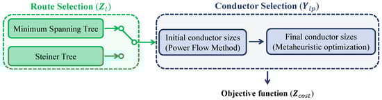
Figure 1.
General framework of the proposed heuristic methodology for optimal expansion of three-phase distribution networks.
The methodology addresses the problem in two main stages—route selection and conductor sizing—each designed to efficiently navigate the solution space while meeting technical and economic constraints. In the first stage, two strategies are explored to define the network topology: the Minimum Spanning Tree [43] and the Steiner Tree [44]. Both ensure radiality and full connectivity.
Once the topology is set, conductor selection is performed in two steps. First, initial sizes are estimated by solving a three-phase power flow using Broyden’s method [45]. These serve as a technically sound baseline. Then, metaheuristic optimization refines the selection to balance investment and energy losses under the model’s constraints. The process concludes with the evaluation of the objective function (), which captures the total annualized cost. This structured, staged approach makes the complex MINLP problem more tractable and suitable for realistic distribution planning.
3.1. Route Selection Strategy
The first step of the methodology defines the network topology by selecting distribution lines that connect all demand nodes while maintaining a radial structure. This configuration directly impacts power flows, voltage drops, current levels, and overall power losses, as well as the total conductor length and associated investment costs. To optimize this stage, two graph-based techniques are employed: the Minimum Spanning Tree (MST) and the Steiner Tree (ST), both aimed at minimizing total network distance.
3.1.1. Minimum Spanning Tree
The MST is a classical algorithm used to connect all nodes in a graph with the minimum total edge length, avoiding cycles [46]. Given a connected undirected graph —where V is the set of nodes, E represents the possible edges or connections, and W denotes the length of the possible connections—the MST is a subgraph, , with edges and minimum total weight [47]. In distribution system planning, the MST provides a radial topology that ensures connectivity while minimizing conductor length. In this study, it is computed using MATLAB’s minspantree function, which builds the MST based on node positions and inter-node distances.
The process is summarized as follows:
- Identify the demand nodes and potential interconnection points based on their spatial coordinates (e.g., geographic location of poles).
- Compute the Euclidean distance between each pair of nodes to assign the weights to the set W.
- Construct the undirected graph and apply the minspantree function to graph, G, which returns a subset of edges, T, forming a tree that connects all nodes with minimum total weight and no loops.
- Use the resulting tree structure as the initial radial topology for the subsequent stage.
In order to illustrate the process of obtaining the MST for a generic system with nodes, consider the following 15-node system, where the loads are spatially distributed as shown in Figure 2. Their geographical coordinates are presented in Table 2. It is important to note that the node locations in this system were randomly generated to demonstrate that the methodology can operate effectively under any scenario.
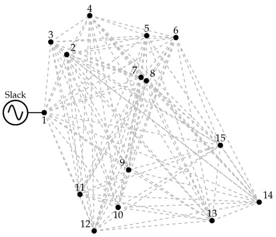
Figure 2.
Fifteen-node distribution systems with all possible routing options.
Table 2.
Spatial location of nodes in the 15-bus test system.
In this case, the graph consists of 15 nodes (V) and 105 possible connections (E). Edge weights (W) or Euclidean distance between each pair of nodes can be efficiently computed using a simple computational routine. Applying the MST algorithm to this graph yields the network configuration illustrated in Figure 3.
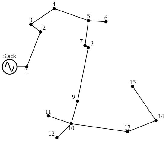
Figure 3.
Radial network topology obtained using the Minimum Spanning Tree approach.
In this case, 14 distribution lines were selected, as detailed in Table 3, resulting in a minimum total network length of 2882.7633 m.
Table 3.
Distribution lines selected by the MST algorithm and their corresponding lengths.
3.1.2. Steiner Tree Approach
Like the MST, the ST is an optimization technique that connects a set of nodes with the shortest possible total distance [48]. However, unlike the MST, the ST allows the inclusion of auxiliary nodes () that enable shorter overall connections between nodes. This results in a radial configuration that minimizes the total line length by combining both demand and auxiliary nodes. In this way, the ST identifies more efficient connections through the strategic placement of , provided that the following conditions are met [48,49].
- Total Steiner points number: The number of added to the system must not exceed . This means that the total number of nodes in the resulting ST is equal to the number of demand nodes plus the number of .
- Node connection criterion: Each can connect to a maximum of three edges. Additionally, only connections between and system nodes, or between two , are permitted. Direct connections between original demand nodes are not allowed, ensuring that all connections in the topology are mediated by at least one .
- Geometric symmetry: The branches connected to each must exhibit geometric symmetry to ensure local minimization of total connection length. Specifically, if a has two connections, the angle between them should be approximately 180°, while in the case of three connections, the angles between adjacent branches should be close to 120°, in accordance with Fermat point geometry.
- Radial configuration: The resulting configuration must be radial (i.e., ), meaning it must contain no loops and must ensure full connectivity among the terminal nodes.
From a computational standpoint, the ST problem is classified as NP-hard, even under simplified conditions [50]. This complexity arises from the need to evaluate a vast number of possible combinations of placements and their associated connections. As the network size increases, finding the exact optimal solution becomes computationally infeasible. However, various heuristic and approximation algorithms have proven effective in delivering high-quality solutions within acceptable time frames [44,51].
To determine the ST topology in this work, a hybrid methodology is proposed that integrates metaheuristic optimization with geometric and graph-theoretic principles. The procedure is structured in two main stages: (i) the optimization of locations using a metaheuristic algorithm, and (ii) the construction of a radial tree based on those locations, ensuring topological and geometric feasibility using the MST-based approach.
Figure 4 illustrates the methodology implemented to determine the ST of a generic system with nodes.
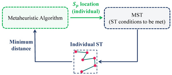
Figure 4.
Heuristic-based methodology for determining the Steiner Tree in a distribution network with nodes.
The methodology presented in Figure 4 can be understood as follows:
- Optimization of locations: The spatial coordinates of the are determined using a metaheuristic known as the Vortex Search Algorithm (VSA) [52]. This algorithm was selected due to its simplicity, ease of implementation on programming tools, and its demonstrated effectiveness in solving both continuous and combinatorial optimization problems.To improve its performance, key parameters of the VSA—such as population size, number of iterations, and the vortex radius decay constant—are tuned in advance using a meta-optimization procedure [53,54]. Each individual within the VSA population represents a candidate solution consisting of specific coordinate positions for the . Each individual of the population has the structure shown in Figure 5.
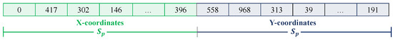 Figure 5. Encoding used by the Vortex Search Algorithm to determine the location of the Steiner points.In this individual, the first elements of the vector represent the X-coordinates of the , while the subsequent elements correspond to their Y-coordinates. This encoding scheme allows the VSA to propose potential locations for the , facilitating the subsequent evaluation of each configuration through the construction and validation of the associated ST. By organizing the coordinates in a structured manner within the solution vector, the process of generating the undirected graph and verifying the required geometric conditions is streamlined.
 - Construction of the Steiner Tree from candidate solutions: For each candidate solution generated by the VSA, a ST is constructed through the following process:
- Construct the undirected graph , where V includes all original demand nodes plus the proposed by the candidate solution; E represents all possible edges. Remember that these possible connections must comply with the connection criterion previously mentioned; W contains the Euclidean distances between all allowed node pairs.
- Identify the best radial structure from this graph. In this case, the minspantree function in MATLAB is applied to generate a MST over the defined graph. This ensures connectivity and minimal total line length.
- After generating the individual ST, a geometric validation step is performed. Trees are discarded if any violates the node connection and geometric symmetry conditions.
Only candidate trees that meet these criteria are considered valid ST. Finally, the iterative process of the VSA is driven by the trees generated by each individual, and ultimately identifies the configuration with the shortest total distance. This configuration is then selected as the network topology for the subsequent conductor sizing stage.
As in the previous case, the ST for the 15-node system depicted in Figure 2 is determined using the procedure described in this section. In this instance, the graph is composed of 28 nodes: 15 demand nodes and 13 Steiner points. Consequently, and in accordance with the connectivity criteria, the graph contains 273 possible edges. The Euclidean distances associated with these connections can be efficiently computed using a simple numerical routine.
By applying the ST-based procedure to this graph, the resulting radial network configuration is obtained, as shown in Figure 6a.
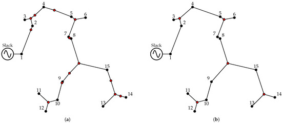
Figure 6.
Radial network topology obtained using: (a) Steiner Tree approach (2705.4084 m); (b) Steiner Tree approach with redundant node elimination (2705.3933 m).
In this case, a total of 27 distribution lines are selected, resulting in a network length of 2705.4084 m. This represents a reduction of 177.3549 m compared to the configuration obtained using the MST. As shown in the ST of Figure 6a, some are positioned along direct paths between nodes or overlap with demand nodes, offering no benefit in reducing total network length. These points typically have only two connections and do not enhance the layout’s efficiency. Therefore, they can be removed without affecting total line length, as illustrated in Figure 6b. This refinement yields a more compact ST with fewer auxiliary points and lines, improving both structural simplicity and efficiency.
The refined ST shown in Figure 6b consists of 20 nodes—15 demand nodes and 5 Steiner points—after removing 8 redundant auxiliary nodes. These points are located at: node 16 (77 m, 863 m), node 17 (451 m, 858 m), node 18 (483 m, 467 m), node 19 (225 m, 119 m), and node 20 (787 m, 191 m). A total of 19 distribution lines are selected, as shown in Table 4, resulting in a network length of 2705.3933 m, which is slightly shorter than the original Steiner configuration, and achieves a reduction of 177.37 m compared to the MST-based layout. A ST is obtained with virtually the same minimal total distance, but with fewer nodes and, more importantly, fewer lines (eight lines are eliminated), which will result in a lower investment cost.
Table 4.
Distribution lines selected by the ST algorithm and their corresponding lengths.
As shown in Figure 6b, the electrical system must incorporate additional nodes—distinct from the original demand nodes—that were not previously considered. These nodes function as branching points, facilitating the interconnection of loads while simultaneously reducing the total conductor length required by the network. Each Steiner point integrated into the system incurs a fixed installation cost of USD 1108.40, which must be included in the overall investment cost of the network expansion (Equation (3)).
3.2. Initial Conductor Sizing
Once the network topology has been defined—either through the MST or the ST approach—the next step is to determine the initial conductor sizes for each distribution line [26]. This stage is essential in providing a starting point for the subsequent optimization phase. The sizing process is based on the evaluation of current flows along the network, obtained by solving a three-phase power flow problem specifically adapted to unbalanced distribution systems.
In this work, the power flow is solved using a numerical approach based on Broyden’s method, which provides an efficient alternative to traditional Jacobian-based techniques. This quasi-Newton approach avoids the explicit calculation and factorization of the Jacobian matrix at each iteration, significantly reducing computational effort while maintaining reliable convergence properties. The selection of Broyden’s method is motivated by its demonstrated advantages in the context of three-phase unbalanced distribution systems, where conventional methods such as Newton–Raphson, iterative backward/forward sweep, and triangular-based techniques often face higher computational costs or slower convergence. As reported in [45], Broyden’s method achieves comparable accuracy to Newton–Raphson. These characteristics make it particularly suitable for the initial conductor sizing stage of the proposed methodology, where efficiency and robustness are essential.
The methodology used to determine the initial conductor sizes is structured as follows:
- Assignment of preliminary conductors for power flow calculation: To compute the current flowing through each line using the Broyden-based power flow method, it is first necessary to assign temporary conductors to the branches of the selected network topology (obtained from the MST or ST). This step is required to define the impedance values associated with each line and, consequently, to enable the numerical solution of the power flow equations.
- Selection of conductor set and parameter definition: A predefined set of eight standard conductor types is considered for use in three-phase distribution systems [55]. For each conductor type, technical and economic parameters are defined, including its thermal current limit and cost per kilometer. These values are summarized in Table 5, while Table 6 presents the corresponding impedance matrices used for the power flow model.
Table 5. Conductor sizes available for the optimal distribution network expansion problem [55].
Table 6. Impedance matrix corresponding to available conductor type [55].
- Initial assumption using the lowest-impedance conductor: For the purpose of approximating the initial current flow as closely as possible to the ideal operating condition, all lines are initially assigned the conductor type with the lowest impedance (conductor 8). This choice minimizes voltage drops along the network and allows for a more realistic estimation of the current absorbed by the loads under ideal conditions.
- Current-based conductor reassignment: Once the power flow is solved and the current magnitudes in each distribution line are obtained, the conductor sizing step continues by comparing these values against the thermal limits of the available conductor types. Specifically, for each line, the maximum current among the three phases is identified and used as the reference for conductor selection. This conservative criterion ensures that, if the highest phase current complies with the thermal limit, the remaining phases—having equal or lower current magnitudes—will also be within safe operating conditions. Consequently, each line is assigned the smallest conductor size capable of supporting the maximum current, ensuring that all branches operate within their thermal capacity while preserving technical feasibility.
To continue illustrating the proposed methodology, we consider again the 15-node test system, using both the MST-based topology (shown in Figure 3) and the ST-based topology (shown in Figure 6b). As observed in both configurations, node 1 is designated as the substation node. It is assumed to operate at a nominal line-to-line voltage of 4.16 kV. The phase-wise load consumption for each demand node in the system is detailed in Table 7. It is important to clarify that the phase-wise load values were also randomly generated. This was performed to demonstrate the robustness of the proposed methodology, showing that it is capable of producing high-quality solutions for any electrical distribution system.
Table 7.
Nodal three-phase load demand profile for the 15-node distribution system.
Using the Broyden-based three-phase power flow method and the load data from Table 7, the current in each phase of every distribution line is calculated, allowing for the initial conductor sizing. Steiner points are modeled as nodes with no power demand, ensuring they do not influence load distribution or distort the power flow, thus preserving the network’s electrical characteristics.
The results of the initial conductor selection are presented in Table 8 for the MST-based topology and the ST configuration.
Table 8.
Initial conductor selection for MST and ST networks in the 15-node system.
3.3. Metaheuristic-Based Optimization
Once the network topology—previously defined using either the MST or ST approach—is known, and the initial conductor sizes have been assigned based on current flow analysis, a refinement stage is carried out to improve the overall performance of the network. To evaluate the objective function and enforce the technical constraints of the optimization model, a master–slave computational strategy is implemented, as shown in Figure 7.
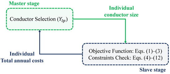
Figure 7.
Master–slave methodology for conductor selection in three-phase distribution networks.
In this framework, the master stage selects conductor sizes starting from an initial configuration and uses metaheuristic algorithms to iteratively explore the discrete solution space, aiming to minimize total annualized cost. The slave stage evaluates each candidate by solving the three-phase power flow via Broyden’s method to obtain voltages and currents, compute the objective function, and verify compliance with all technical constraints—such as voltage bounds, thermal limits, radiality, and power balance. Infeasible solutions are discarded accordingly.
To solve the combinatorial conductor selection problem, this work employs four population-based metaheuristic algorithms: the Chu–Beasley Genetic Algorithm(CBGA) [56], Particle Swarm Optimization (PSO) [57], the Sine–Cosine Algorithm (SCA) [58], and the Grey Wolf Optimizer (GWO) [59]. These algorithms are well-suited for exploring large, discrete, and nonlinear search spaces, such as the one defined by the conductor sizing problem in unbalanced three-phase networks. It is worth noting that readers are encouraged to consult the original references of each algorithm (cited alongside their names) for a detailed explanation of their structure, inspiration, and parameter influence, since the present work focuses on their application to the distribution network planning problem.
Although each algorithm has distinct mechanisms for guiding the search process, they generally follow a common optimization structure composed of the following steps:
- Initial solution generation: The optimization starts by generating an initial population of candidate solutions, where each individual represents a complete conductor assignment for the active lines of the selected topology (MST or ST); while purely random initialization can promote diversity, in this study the conductor configuration obtained from the preliminary power flow analysis is used as the starting point. This ensures technical feasibility from the outset and provides a solid baseline for subsequent refinement.Each individual in the population is encoded as a discrete integer vector (Figure 8), where the vector length equals the total number of distribution lines in the topology. Each element corresponds to a specific line and stores an integer indicating the selected conductor type, chosen from the set of available options (Table 5). This encoding guarantees a direct and unambiguous mapping between decision variables and physical network elements.
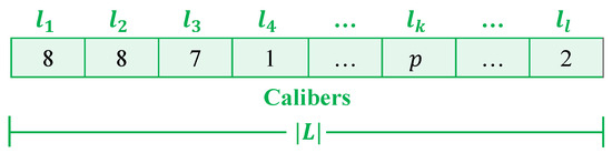 Figure 8. Encoding used by the metaheuristic algorithms to determine the conductor sizes for each enabled line.
 - Exploration and exploitation (search process): At each iteration, the metaheuristic algorithm balances two complementary tasks: exploration, which promotes diversity by visiting unexplored regions of the search space, and exploitation, which intensifies the search around promising solutions already identified. This balance is regulated by algorithm-specific parameters (e.g., crossover and mutation rates in CBGA, inertia weight in PSO, control parameters in SCA, or exploration factor in GWO), which were set according to widely used values reported in the literature.More specifically:
- In the CBGA, exploration is driven by the crossover operator (), which recombines genetic material from two parents to generate offspring with hybrid traits. Exploitation is supported by a mutation operator (), which introduces small perturbations that refine promising regions while preserving diversity.
- In PSO, exploration is governed by the inertia weight, w, which decreases linearly from to across iterations, enabling a wide search early on and faster convergence later. Exploitation is guided by the acceleration coefficients (), which balance individual learning (cognitive term) and collective learning (social term).
- In the SCA, candidate solutions are updated using sine and cosine functions, with the control parameter decreasing linearly from 2 to 0 over the iterations. This dynamic adjustment allows the algorithm to emphasize global exploration in the initial stages and gradually transition to local exploitation.
- In the GWO, exploration and exploitation are modeled through the hierarchical hunting process led by three leaders (, , and ). The exploration coefficient, a, decreases linearly from 2 to 0 as iterations progress, reducing randomness and progressively focusing the search around the best solutions identified.
These parameterizations regulate the balance between exploration and exploitation in each method, directly influencing convergence speed, robustness, and solution diversity, and were carefully selected to ensure fairness in the comparative analysis. - Best solution update: After evaluating the objective function of all individuals via the master–slave framework, the best-performing solution is updated and preserved. Each algorithm employs a different mechanism to ensure this:
- In CBGA, elitism ensures that the best individual is carried forward to the next generation.
- In PSO, each particle tracks its own best solution while the global best guides the swarm.
- In SCA, the best candidate is continuously used as a reference for the trigonometric transformations that update other solutions.
- In GWO, the hierarchical structure ensures that (global best) is preserved while and contribute to guiding the rest of the population.
In all cases, the best feasible solution found so far is guaranteed to be retained and reported at the end of the optimization process. - Stopping criterion: The iterative process continues until a stopping condition is satisfied. In this study, a fixed maximum of 1000 iterations was adopted, with a population size of 20 individuals for all algorithms, ensuring fair comparison across methods. The convergence threshold was implicitly monitored by tracking the evolution of the best cost function value. If no improvement occurred over a significant number of iterations, the algorithm naturally converged before the maximum iteration count.
4. Test Feeder
To assess the effectiveness of the proposed methodology, two test cases are considered: the numerical example presented in Section 3 (15-node system) and a 25-node test feeder. The main characteristics and data for both systems are described below. These systems enable a comparative analysis of the routing strategies (MST and ST), the accuracy of the initial conductor sizing based on power flow analysis, and the improvement achieved through metaheuristic optimization.
4.1. Fifteen-Node Distribution System
This system corresponds to the same 15-node distribution system previously used in Section 3 to illustrate the proposed optimization methodology.
4.2. Twenty-Five-Node Distribution System
The 25-node test system is a system that operates at a line-to-line voltage of 4.16 kV and consists of 25 nodes and 24 loads. The spatial distribution of the loads is shown in Figure 9 and their geographical coordinates are presented in Table 9. It is important to note that this system has 300 possible connections for the MST and 828 possible connections for the ST.
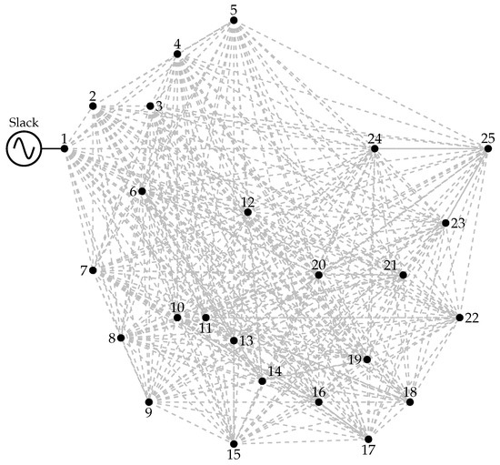
Figure 9.
Twenty-five-node distribution systems with all possible routing options.
Table 9.
Spatial location of nodes in the 25-bus test system.
It is important to mention that, as with the 15-node system, both the node locations and the phase-wise power demands were randomly generated to demonstrate the effectiveness of the proposed methodology.
The phase-wise load consumption for each demand node in the system is detailed in Table 10.
Table 10.
Nodal three-phase load demand profile for the 25-node distribution system.
4.3. Fifty-Node Distribution System
The 50-node test system is a system that operates at a line-to-line voltage of 6.6 kV and consists of 50 nodes and 49 loads. The spatial distribution of the loads is shown in Figure 10 and their geographical coordinates are presented in Table 11. It is important to note that this system has 1225 possible connections for the MST and 1891 possible connections for the ST.
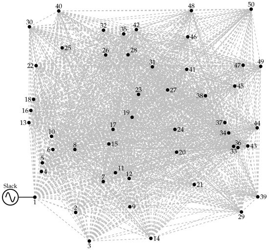
Figure 10.
Fifty-node distribution systems with all possible routing options.
Table 11.
Spatial location of nodes in the 50-bus test system.
It is important to mention that, as with the 15- and 25-node systems, both the node locations and the phase-wise power demands were randomly generated to demonstrate the effectiveness of the proposed methodology.
The phase-wise load consumption for each demand node in the system is detailed in Table 12.
Table 12.
Nodal three-phase load demand profile for the 50-node distribution system.
Similarly, to determine the value of the objective functions defined in (1) and (3), the parametric information shown in Table 13 was used.
Table 13.
Parametric information used for the system cost calculations [34].
5. Numerical Results and Discussions
This section presents the computational results obtained by applying the proposed heuristic methodology to the test systems described previously. The aim is to evaluate the performance of each component of the approach—route selection, initial conductor sizing, and metaheuristic optimization—across different network configurations and load scenarios. The comparative analysis focuses on the total annualized cost, network length, and compliance with technical constraints, under both the MST and the ST topologies. For the computational implementation of the proposed methodology, all scripts were developed in MATLAB R2024a. The simulations were executed on a workstation equipped with a 12th Gen Intel Core i7-12700T CPU @ 1.40 GHz, 32 GB of RAM, running 64-bit Windows 11 Pro.
5.1. Fifteen-Node Distribution System
The results of the proposed routing methodology are shown in Figure 3 for the MST and Figure 6b for the ST. Based on each topology, initial conductor sizes are assigned using current flow analysis (Table 8), serving as starting points for the metaheuristic optimization. The final results are summarized in Table 14, which reports the total annualized cost (), the energy loss cost (), and the investment cost () for both topologies. The first two rows show the initial configurations, and the remaining rows correspond to the optimized solutions obtained via four metaheuristic algorithms.
Table 14.
Numerical results for the 15-node distribution system.
From Table 14, the following can be analyzed:
- Energy loss costs are a key component of the objective function, especially in the initial configurations. The MST-based solution shows the highest value (USD 185,628.55), followed by the initial ST configuration (USD 151,919.49), both using low-caliber, high-impedance conductors. Optimized solutions significantly reduce , with ST-based methods consistently outperforming MST-based ones. The ST-SCA solution achieves the lowest loss cost (USD 37,229.69), driven by the frequent selection of high-capacity conductors (e.g., caliber 8), which minimize resistive losses on heavily loaded lines.
- The initial MST and ST configurations show low investment costs—USD 51,883.49 and USD 50,927.83—due to uniform use of small, low-cost conductors. However, these setups lack technical efficiency. Optimized solutions increase investment, especially in MST-based cases (USD 205,935.15 to USD 208,785.75), driven by widespread use of high-caliber conductors (types 7 and 8) to reduce losses. ST-based solutions, despite including USD 5542.00 for five Steiner points, maintain lower costs (USD 182,312.43 to USD 194,146.64). This is largely due to the shorter network length—2705.39 m vs. 2882.76 m for the MST—which reduces material usage and overall capital needs, while enhancing energy and economic efficiency.
- Total cost reflects both conductor investment and energy losses. The initial MST and ST configurations present the highest values—USD 222,689.91 and USD 183,245.15—underscoring the need for optimization. After applying metaheuristics, costs drop notably, with ST-GA and ST-GWO achieving the lowest total cost (USD 65,401.37). This is due to the efficient ST layout and strategic use of conductors—reserving high-capacity types (e.g., calibers 7 and 8) for critical lines while using cheaper options elsewhere—striking a balance between loss reduction and investment.
Table 15 presents a comparative summary of the numerical performance of the four metaheuristic algorithms applied to the 15-node system, based on 100 consecutive runs for each method. The table reports the best, mean, and worst total cost solutions, along with the standard deviation and average execution time. Results are shown for both MST and ST topologies, allowing for an assessment of each algorithm’s quality, robustness, and computational efficiency.
Table 15.
Numerical performance obtained for the 15-node distribution system.
From Table 15, the following can be analyzed:
- The best solutions confirm that the ST-based configurations consistently outperform those using the MST topology. The lowest total cost is achieved by both ST-GA and ST-GWO, each with a best solution of USD 65,401.37. Among the MST-based approaches, the lowest best solution is USD 73,622.61, obtained by both MST-GA and MST-GWO. These results emphasize the advantage of the ST layout in reducing system costs when combined with effective metaheuristic optimization.
- The average performance over 100 runs confirms the same trend: ST-based algorithms yield lower mean costs, with ST-GWO achieving the lowest and most consistent average at USD 65,401.73, followed closely by ST-GA. In contrast, MST-based methods show higher mean costs—particularly MST-PSO (USD 92,803.89) and MST-SCA (USD 84,053.34)—reflecting less consistent performance. These results reaffirm that ST-based methods, especially ST-GWO, consistently achieve better and more reliable solutions.
- The worst-case results further confirm the robustness of the ST-based methods. ST-GWO stands out, achieving the lowest worst-case cost at USD 65,433.53, closely followed by ST-GA with USD 65,512.44. In contrast, MST-PSO shows a substantial gap, reaching USD 148,495.99, reflecting high sensitivity to initial conditions. Overall, ST-based strategies—especially ST-GWO—offer consistent and reliable performance with minimal deviation from optimality.
- ST-GWO shows the highest repeatability, with a minimal deviation of 0.00494%. ST-GA and MST-GWO also perform consistently, both below 0.1%. In contrast, MST-PSO and MST-SCA exhibit high variability (15.51% and 4.17%), indicating reduced reliability. These results underscore the robustness of the ST topology, especially when paired with GWO.
- In terms of computational efficiency, ST-GA is the fastest, averaging 11.54 s, followed by MST-GA (14.72 s) and ST-GWO (27.56 s). The slowest methods are MST-PSO (84.59 s) and MST-SCA (77.25 s), reflecting a higher computational load in MST-based searches. These results indicate that ST-based approaches, especially when paired with GA or GWO, not only achieve better solutions but also offer superior or comparable run time performance.
5.2. Twenty-Five-Node Test Feeder
By applying the same procedure used for the 15-node system, as described in Section 3, to the 25-node distribution system, the resulting MST and ST topologies are obtained and shown in Figure 11.
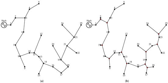
Figure 11.
Optimal route selection in the 25-node distribution system: (a) topology provided by the MST (2993.62 m); (b) topology provided by the ST (2850.35 m).
Figure 11 shows that both topologies maintain a radial structure. In the case of the MST, the 25 demand nodes are connected through 24 lines, resulting in a minimum total length of 2993.62 m. In contrast, the ST topology incorporates 11 Steiner points (which represents fixed costs of USD 12,192.40), yielding a total of 36 nodes and 35 lines, with a reduced total length of 2850.35 m. This represents a reduction of 143.27 m compared to the MST, highlighting the efficiency of the Steiner Tree in minimizing the overall network distance.
The specific locations of the 11 Steiner points are as follows: node 26 at (837 m, 419 m), node 27 at (84 m, 319 m), node 28 at (657 m, 149 m), node 29 at (685 m, 118 m), node 30 at (150 m, 520 m), node 31 at (668 m, 260 m), node 32 at (63 m, 550 m), node 33 at (413 m, 155 m), node 34 at (342 m, 256 m), node 35 at (179 m, 199 m), and node 36 at (818 m, 327 m).
By applying the Broyden-based three-phase power flow method to both the MST and ST topologies—using the load values reported in Table 10—the corresponding initial conductor sizes can be determined. The results of the initial conductor selection for the MST-based and ST-based topologies are presented in Table 16.
Table 16.
Initial conductor selection for MST and ST networks in the 25-node system.
Once the topology and initial conductors are defined, the solution is refined using metaheuristic optimization techniques. Table 17 presents the results for the 25-node test system and follows the same structure as in the 15-node case.
Table 17.
Numerical results for the 25-node distribution system.
From this table the following can be analyzed:
- Energy loss costs are significantly higher in the initial configurations, particularly for the MST (USD 137,835.86), due to the predominant use of low-caliber conductors with high impedance. Although the ST topology also begins with smaller conductor sizes, it achieves lower initial losses (USD 117,538.06). After optimization, all methodologies significantly reduce . The best result is achieved by ST-GWO (USD 52,125.82), followed by ST-GA (USD 52,746.43), both of which are characterized by the efficient allocation of high-caliber conductors (types 7 and 8) on critical lines. In contrast, MST-PSO yields the worst optimized outcome (USD 61,022.76), indicating a lower capacity to balance power losses and investment costs.
- Investment costs differ notably across approaches. The initial MST setup incurs a high cost (USD 70,854.11) due to mixed, often expensive conductors. In contrast, the initial ST configuration achieves the lowest cost (USD 33,497.97), benefiting from shorter network length and widespread use of low-cost conductors, despite including 11 Steiner points. Optimized MST solutions require higher investments (USD 155,180.70–USD 164,949.03) due to heavy use of large calibers. ST-based solutions, while also using high-capacity conductors strategically, keep costs lower—e.g., ST-SCA (USD 128,715.99) and ST-GWO (USD 150,938.44), both including the USD 12,192.40 cost of Steiner nodes. This reflects the ST’s structural efficiency in minimizing conductor usage.
- The initial MST configuration shows the highest cost (USD 169,152.56), followed by the initial ST setup (USD 163,228.42), both unoptimized. After applying metaheuristics, total costs drop significantly. ST-based solutions deliver the best outcomes, with ST-GWO achieving the lowest value (USD 79,319.81), closely followed by ST-GA (USD 79,377.57). This is due to a balanced use of high-capacity conductors on critical paths and economical ones elsewhere, alongside reduced losses. Optimized MST configurations yield higher costs—MST-GA and MST-GWO perform best among them (USD 89,340.67 each), yet remain well above their ST counterparts. These results confirm the economic advantage of the Steiner Tree approach, which reduces both operating and investment costs through a more compact and flexible layout.
Table 18 presents the numerical performance of the metaheuristic algorithms applied to the 25-node test system, following the same structure and evaluation criteria used in Table 15.
Table 18.
Numerical performance obtained for the 25-node distribution system.
From Table 18, the following can be analyzed:
- The best total costs again favor ST-based methods. ST-GWO achieves the lowest value (USD 79,319.81), closely followed by ST-GA (USD 79,377.57), confirming the superior performance of the ST configuration. MST-based methods deliver consistently higher costs, with MST-GA and MST-GWO achieving the best values among them (both at USD 89,340.67), indicating that MST topology is less effective in minimizing total cost.
- The mean results reinforce the trend observed in the best solutions. ST-GWO records the lowest average cost (USD 79,355.03), demonstrating not only optimal performance but also remarkable consistency across executions. ST-GA follows with USD 80,066.64, while MST-based methods show higher averages, particularly MST-PSO (USD 101,331.51) and MST-SCA (USD 108,502.28), indicating greater variability and less reliability in their outcomes.
- Worst-case results highlight the robustness of each method. ST-GWO maintains strong performance with a worst solution of USD 79,804.83, just slightly above its best. Similarly, ST-GA and ST-SCA also show contained variation. In contrast, MST-PSO and MST-SCA reach significantly higher worst values (USD 154,982.50 and USD 140,437.11), indicating high sensitivity to initial conditions and less dependable performance.
- Regarding standard deviation, ST-GWO shows the lowest deviation (0.096%) among all methods, confirming its excellent stability. Although MST-GWO also performs well (0.0826%), it does so at a higher cost. ST-GA maintains good consistency (0.467%), while MST-PSO (11.39%) and ST-SCA (9.35%) show high variability and less reliable convergence. Overall, ST-GWO strikes the best balance between robustness and solution quality, making it the most dependable strategy tested.
- Execution times show a clear trade-off between solution quality and computational cost. ST-GA is the fastest among ST methods (29.44 s), followed by MST-GA (17.35 s), while ST-GWO (150.05 s) and ST-PSO (151.50 s) require more time to converge. Despite the longer run times, ST-GWO delivers the most consistent and cost-effective results, validating its robustness for practical applications.
5.3. Fifty-Node Test Feeder
By applying the same procedure used for the 15- and 25-node systems, as described before, to the 50-node distribution system, the resulting MST and ST topologies are obtained and shown in Figure 12.
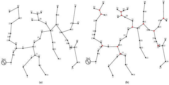
Figure 12.
Optimal route selection in the 50-node distribution system: (a) topology provided by the MST (24,734.69 m); (b) topology provided by the ST (24,095.77 m).
Figure 11 shows that both topologies maintain a radial structure. In the case of the MST, the 50 demand nodes are connected through 49 lines, resulting in a minimum total length of 24,734.69 m. In contrast, the ST topology incorporates 12 Steiner points (which represents fixed costs of USD 13,300.80), yielding a total of 62 nodes and 61 lines, with a reduced total length of 24,095.77 m. This represents a reduction of 638.92 m compared to the MST, highlighting the efficiency of the Steiner Tree in minimizing the overall network distance.
The specific locations of the 12 Steiner points are as follows: node 51 at (1798 m, 4160 m), node 52 at (4156 m, 2016 m), node 53 at (1823 m, 3943 m), node 54 at (3220 m, 3400 m), node 55 at (3891 m, 2950 m), node 56 at (596 m, 2010 m), node 57 at (521 m, 4017 m), node 58 at (2518 m, 3194 m), node 59 at (1572 m, 1954 m), node 60 at (4501 m, 3752 m), node 61 at (1740 m, 1495 m), and node 62 at (423 m, 4273 m).
By applying the Broyden-based three-phase power flow method to both the MST and ST topologies—using the load values reported in Table 12—the corresponding initial conductor sizes can be determined. The results of the initial conductor selection for the MST-based and ST-based topologies are presented in Table 19.
Table 19.
Initial conductor selection for MST and ST networks in the 50-node system.
Once the topology and initial conductors are defined, the solution is refined using metaheuristic optimization techniques. Table 20 presents the results for the 50-node test system and follows the same structure as in the 15- and 25-node cases.
Table 20.
Numerical results for the 50-node distribution system.
From this table the following can be analyzed:
- Energy losses are noticeably higher in MST-based configurations, reaching up to USD 298,393.19 in MST-SCA, reflecting the intensive use of smaller-caliber conductors over long feeders. With refinement, the most efficient methods achieve significant reductions: MST-GA and MST-GWO stand out with USD 259,533.27 and USD 263,079.97,, respectively. In contrast, ST-based configurations show higher values, around USD 335,011.38 in ST-SCA and ST-PSO, due to the larger number of lines required to incorporate Steiner nodes. However, ST-GWO partially compensates for this effect, reaching USD 258,371.31—the lowest value among all configurations—confirming its ability to mitigate losses through the strategic allocation of large-caliber conductors on critical branches.
- Investment in conductors shows marked differences. Among the MST methods, costs range between USD 817,179.55 (MST-GWO) and USD 855,439.72 (MST-GA), reflecting the need for larger conductors to meet technical constraints in longer topologies. ST configurations, despite reducing network length, exhibit similarly high investments (around USD 848,659.71 in ST-SCA/PSO), though with lower dispersion. The most efficient case corresponds to ST-GA with USD 813,153.60, which achieves a significant reduction by optimizing conductor allocation in combination with the more compact Steiner Tree topology.
- The global analysis confirms the superiority of ST-based solutions compared to MST ones. The lowest total cost is obtained by ST-GWO (USD 411,224.67), closely followed by MST-GWO (USD 412,953.40) and MST-GA (USD 413,309.05). These results show that, although MST can achieve competitive performance when combined with efficient metaheuristics, the topological flexibility of the Steiner Tree enables the most cost-effective outcomes. In contrast, ST-SCA and ST-PSO present much higher costs (USD 502,014.39), indicating a lower ability of these heuristics to balance losses and investment costs in large systems.
The relatively close results observed between MST- and ST-based methodologies in the 50-node case can be explained by the substantial growth of the solution space compared to the 15- and 25-node systems. In particular, the ST configurations expand to 62 nodes due to the inclusion of 12 additional Steiner nodes, which significantly enlarges the search space and increases the difficulty of finding globally competitive solutions. This effect causes the ST-based methods to occasionally lose performance relative to MST-based approaches, despite their topological advantages. These findings suggest that, for larger systems, preliminary tuning stages—such as parameter calibration or hybrid initialization strategies—are necessary to improve the search efficiency of metaheuristic algorithms and fully exploit the structural benefits of the Steiner Tree formulation.
Table 21 presents the numerical performance of the metaheuristic algorithms applied to the 50-node test system, following the same structure and evaluation criteria used in Table 15.
Table 21.
Numerical performance obtained for the 50-node distribution system.
From Table 21, the following can be analyzed:
- The average results again highlight the robustness of the GWO-based approaches. MST-GWO achieves the lowest mean cost (USD 417,212.60), followed closely by ST-GWO (USD 435,934.97). These values demonstrate not only good performance but also consistent convergence. By contrast, ST-SCA (USD 557,350.40) and ST-PSO (USD 472,983.47) show significantly higher averages, indicating less reliable optimization behavior across multiple runs.
- The worst-case outcomes provide further insight into algorithm robustness. MST-GWO (USD 456,221.31) and MST-GA (USD 457,592.96) maintain strong performance even in their least favorable iterations, while ST-GWO also contains variability with 499,227.15 USD. On the other hand, ST-PSO (USD 640,938.88) and ST-SCA (USD 621,407.88) deteriorate substantially under adverse conditions, showing limited resilience in larger search spaces.
- Variability across runs is lowest for MST-GWO (1.293%) and MST-GA (2.093%), demonstrating stable convergence. ST-GA (5.464%) also shows acceptable consistency. However, ST-PSO (12.504%) and ST-SCA (6.755%) present high variability, confirming their weaker robustness in the 50-node case. ST-GWO remains competitive with a deviation of 3.567%, balancing solution quality and reliability.
- In terms of computational effort, MST-GA is by far the fastest method (236.37 s), followed by MST-GWO and MST-PSO (2900 s each). ST-based methods, however, require longer run times, with ST-GA (715.40 s) being the most efficient among them, while ST-PSO (7248.53 s) and ST-SCA (5974.49 s) are the most computationally demanding. Despite the longer times, ST-GWO (4815.45 s) delivers the best balance between cost efficiency, robustness, and scalability, validating it as the most dependable approach for practical planning applications.
The simulation results for the 15-, 25- and 50-node systems clearly demonstrate the superior performance of the ST-GWO configuration. This method consistently achieved the lowest total costs, along with outstanding robustness and repeatability, confirming its effectiveness in balancing energy loss reduction and investment minimization; while ST-GWO requires longer computational times than other methods, this is not a significant drawback in distribution network planning, where solutions are computed offline and optimality is prioritized over speed.
The proposed methodology is inherently scalable, as it separates the overall problem into modular stages—route selection, initial conductor sizing, and metaheuristic refinement. Each stage is computationally tractable and benefits from algorithmic parallelization or preprocessing techniques (e.g., the use of MST or ST heuristics to reduce the search space). Moreover, the use of discrete encoding for conductors, combined with a master–slave architecture, enables the flexible adaptation to different system sizes, phases, and operational constraints. Thanks to this structure, the methodology can be extended to large-scale systems with over 100 nodes, provided that appropriate computational resources are allocated. This opens the possibility for its application in real-world rural and semi-urban distribution networks, where the complexity of the planning problem increases substantially with system size.
From a practical standpoint, the methodology can be directly applied to real-world distribution systems, as it considers key technical constraints such as voltage regulation, thermal limits, and radial topology enforcement. Additionally, the integration of geographic information (e.g., pole coordinates), realistic conductor sizes, and demand profiles makes it compatible with data routinely available to utilities. These features position the proposed ST-GWO-based approach as a powerful decision-support tool for the cost-effective and technically sound planning of unbalanced three-phase rural networks.
5.4. Environmental Sustainability of the Proposed Solutions
In addition to the economic evaluation, it is important to analyze the environmental impact associated with the proposed planning strategies. In this subsection, the sustainability of the solutions is assessed by estimating the emissions resulting from the energy generation of the distribution systems. For this purpose, an emission factor of 0.2671 kg/kWh is adopted for rural systems [60], which enables the environmental cost of the proposed solutions to be quantified.
For each test system, both the best and the worst solutions obtained with the proposed methodology are examined. This comparative approach highlights how different planning decisions influence the magnitude of emissions, and provides insights into the trade-offs between technical efficiency, economic cost, and environmental sustainability.
Table 22 presents the estimated emissions derived from the daily energy generation of the best solutions obtained for each test system. The values illustrate how different planning strategies influence the environmental impact, particularly as system size increases.
Table 22.
Estimated emissions associated with the worst and best solutions obtained for each test system.
From Table 22, the following can be analyzed:
- Fifteen-node system: Both methodologies yield very similar environmental performance. MST-SCA produces 11,036.68 kg, while ST-GWO slightly improves the outcome with 11,012.81 kg. The marginal difference reflects that, in small networks, the choice of topology and optimization method has limited influence on total emissions, since losses are constrained by the relatively short feeder lengths.
- Twenty-five-node system: The impact of methodology becomes more noticeable. MST-SCA results in 16,866.65 kg, whereas ST-GWO achieves a reduction to 16,797.70 kg. Although the numerical difference remains modest, it illustrates the capacity of the Steiner Tree configuration to marginally improve efficiency and thus mitigate emissions as system size and complexity increase.
- Fifty-node system: The environmental differences are amplified in larger networks. ST-SCA reports the highest emission value (30,251.52 kg), reflecting its higher operational losses under this configuration. Conversely, ST-GWO attains the lowest value (29,848.04 kg), achieving a reduction of over 400 kg compared to ST-SCA. This demonstrates that the choice of optimization method has a measurable effect on environmental sustainability in large-scale systems, with GWO showing superior capacity to balance network efficiency and emissions.
The analysis of emissions confirms that the proposed planning methodology not only reduces investment and operational costs but also contributes to environmental sustainability; while differences between methods are marginal in small systems, they become increasingly relevant as network size grows, with ST-GWO consistently achieving the lowest emission levels. This outcome highlights the importance of adopting optimization strategies that minimize energy losses, since even moderate reductions translate into significant emission savings over the system’s lifetime. In this way, the proposed methodology supports the United Nations Sustainable Development Goals (SDGs), particularly SDG 7 (Affordable and Clean Energy) by improving access to efficient electrification, and SDG 13 (Climate Action) by mitigating the climate impact associated with electricity distribution losses.
6. Conclusions and Future Research Directions
This article presents a comprehensive optimization methodology for the joint routing and conductor sizing problem in unbalanced three-phase distribution networks. The approach integrates the generation of radial topologies (MST and ST), initial conductor allocation based on current flow analysis using the Broyden method, and refinement through four metaheuristic algorithms: CBGA, SCA, PSO, and GWO. The complete framework was validated on 15-, 25- and 50-node rural distribution systems.
The numerical results confirm the superiority of the Steiner Tree combined with the Grey Wolf Optimizer (ST-GWO), which achieved the lowest total cost in the test systems: USD 65,401.37 in the 15-node case, USD 79,319.81 in the 25-node case, and USD 411,224.67 in the 50-node case. Furthermore, ST-GWO exhibited the highest repeatability, with minimal standard deviations of only 0.0049%, 0.096%, and 3.5673% respectively. These results underscore not only the effectiveness and robustness of the method but also its reliability and practical viability for medium- and long-term distribution network planning under unbalanced operating conditions.
Looking ahead, several specific research directions are envisioned to further enhance the proposed methodology. First, the incorporation of hourly or seasonal demand curves is suggested to capture the temporal variability of electrical loads, although this will introduce additional data and modeling complexity that must be carefully addressed. Second, the integration of renewable energy sources, such as photovoltaic and wind systems, is proposed, including the evaluation of their optimal placement and sizing within the expanded network; the stochastic nature of these sources poses challenges in maintaining system stability and requires more advanced modeling. Third, the inclusion of battery energy storage systems is recommended to efficiently manage energy under high renewable penetration, which also demands coordinated operation strategies and degradation modeling. Fourth, the application of stochastic and robust optimization techniques is identified as a promising extension, as they would enable explicit treatment of uncertainties in demand growth and renewable generation, thereby improving the adaptability and reliability of the expansion plans; however, such methods may significantly increase computational complexity, which could be mitigated through parallel computing or decomposition approaches. Finally, extending the methodology to larger and more complex distribution systems is proposed, incorporating additional operational constraints such as voltage control, power flow regulation, and protection coordination, which would strengthen the practical applicability of the framework to real-world networks.
Author Contributions
Conceptualization, methodology, software, and writing (review and editing): L.M.R.-E., B.C.-C., O.D.M., L.F.G.-N. and J.C.H. All authors have read and agreed to the published version of the manuscript.
Funding
The authors acknowledge the support provided by Thematic Network 723RT0150, i.e., Red para la integración a gran escala de energías renovables en sistemas eléctricos (RIBIERSE-CYTED), funded through the 2022 call for thematic networks of the CYTED (Ibero-American Program of Science and Technology for Development).
Institutional Review Board Statement
Not applicable.
Informed Consent Statement
Not applicable.
Data Availability Statement
The original contributions presented in this study are included in the article. Further inquiries can be directed to the corresponding author.
Conflicts of Interest
The authors declare no conflicts of interest.
References
- Hincapié, R.A.; Granada, M.; Gallego, R.A. Optimal planning of the electrical system of the city of Pereira using an exact mathematical methodology. Rev. Ing. 2008, 28, 51–58. (In Spanish) [Google Scholar] [CrossRef]
- Herrera-Cisneros, E.B.; Inga-Ortega, E.M. Optimal planning of overhead distribution networks based on graph theory. Iteckne 2018, 15, 122–130. (In Spanish) [Google Scholar] [CrossRef]
- Gallegos, J.; Arévalo, P.; Montaleza, C.; Jurado, F. Sustainable electrification—Advances and challenges in electrical-distribution networks: A review. Sustainability 2024, 16, 698. [Google Scholar] [CrossRef]
- Vahidinasab, V.; Tabarzadi, M.; Arasteh, H.; Alizadeh, M.I.; Beigi, M.M.; Sheikhzadeh, H.R.; Mehran, K.; Sepasian, M.S. Overview of electric energy distribution networks expansion planning. IEEE Access 2020, 8, 34750–34769. [Google Scholar] [CrossRef]
- Ehnberg, J.; Ahlborg, H.; Hartvigsson, E. Approach for flexible and adaptive distribution and transformation design in rural electrification and its implications. Energy Sustain. Dev. 2020, 54, 101–110. [Google Scholar] [CrossRef]
- Gadelha Filho, T.; Silvia, C.; Aleksandar, D.; Massimo, B.; Marco, M. Rural electrification planning based on graph theory and geospatial data: A realistic topology oriented approach. Sustain. Energy Grids Netw. 2021, 28, 100525. [Google Scholar] [CrossRef]
- Gaurav, A.; Tyagi, A.; Jha, S.; Kumar, B. Optimal sizing and economic assessment of grid connected active distribution network for reliable rural electrification in India. Energy Convers. Manag. 2024, 311, 118505. [Google Scholar] [CrossRef]
- Rastgou, A. Distribution network expansion planning: An updated review of current methods and new challenges. Renew. Sustain. Energy Rev. 2024, 189, 114062. [Google Scholar] [CrossRef]
- Agajie, T.F.; Khan, B.; Alhelou, H.H.; Mahela, O.P. Optimal expansion planning of distribution system using grid-based multi-objective harmony search algorithm. Comput. Electr. Eng. 2020, 87, 106823. [Google Scholar] [CrossRef]
- Gallego Pareja, L.A.; López-Lezama, J.M.; Gómez Carmona, O. Optimal integration of distribution network reconfiguration and conductor selection in power distribution systems via MILP. Energies 2023, 16, 6998. [Google Scholar] [CrossRef]
- Yaima, O.R. Indicative Expansion Plan for Electricity Coverage Extension; UPME: Bogotá, Colombia, 2016. (In Spanish) [Google Scholar]
- Alfaro, J.F.; Miller, S.A. Analysis of electrification strategies for rural renewable electrification in developing countries using agent-based models. Energy Sustain. Dev. 2021, 61, 89–103. [Google Scholar] [CrossRef]
- Karamov, D.N.; Ilyushin, P.V.; Suslov, K.V. Electrification of rural remote areas using renewable energy sources: Literature review. Energies 2022, 15, 5881. [Google Scholar] [CrossRef]
- Minas, A.M.; García-Freites, S.; Walsh, C.; Mukoro, V.; Aberilla, J.M.; April, A.; Kuriakose, J.; Gaete-Morales, C.; Gallego-Schmid, A.; Mander, S. Advancing Sustainable Development Goals through energy access: Lessons from the Global South. Renew. Sustain. Energy Rev. 2024, 199, 114457. [Google Scholar] [CrossRef]
- Ashraf, M.S.; Ahmed, F.; Kousar, S.; Ferreira, P.J.S.; de Almeida, D.M.F. People Category of UN SDGs 2030 and Sustainable Economic Growth in Asia and the Pacific Region. Sustainability 2024, 16, 7950. [Google Scholar] [CrossRef]
- Purnomo, S.; Purwandari, S. A Comprehensive Micro, Small, and Medium Enterprise Empowerment Model for Developing Sustainable Tourism Villages in Rural Communities: A Perspective. Sustainability 2025, 17, 1368. [Google Scholar] [CrossRef]
- Cojocaru, T.M.; Ionescu, G.H.; Firoiu, D.; Cismaș, L.M.; Oțil, M.D.; Toma, O. Reducing Inequalities within and among EU Countries—Assessing the Achievement of the 2030 Agenda for Sustainable Development Targets (SDG 10). Sustainability 2022, 14, 7706. [Google Scholar] [CrossRef]
- Mulero, L.; Grau, D.; Cunill, J.; Fàbregas, A.; Rossell, J.M. Promoting and Prioritizing the Sustainable Development Goals in Young People. Sustainability 2024, 16, 10813. [Google Scholar] [CrossRef]
- Cuenca-Enrique, C.; del Río-Carazo, L.; Acquila-Natale, E.; Iglesias-Pradas, S. Sustainability of Rural Electrification Projects in Developing Countries: A Systematic Literature Review. Energies 2024, 17, 5925. [Google Scholar] [CrossRef]
- Hernández, L.P.; Franco, J.F.; Gallego, R.A. Distribution system planning using tabu search. Sci. Tech. 2007, 13, 85–90. Available online: https://hdl.handle.net/11059/212 (accessed on 19 June 2025). (In Spanish).
- Lavorato, M.; Franco, J.F.; Rider, M.J.; Romero, R. Imposing radiality constraints in distribution system optimization problems. IEEE Trans. Power Syst. 2011, 27, 172–180. [Google Scholar] [CrossRef]
- Montoya, O.; Grajales, A.; Hincapié, R.; Granada, M.; Gallego, R. Methodology for optimal distribution system planning considering automatic reclosers to improve reliability indices. In Proceedings of the 2014 IEEE PES Transmission & Distribution Conference and Exposition-Latin America (PES T&D-LA), Medellin, Colombia, 10–13 September 2014; IEEE: Piscataway, NJ, USA, 2014; pp. 1–6. [Google Scholar] [CrossRef]
- Koutsoukis, N.; Georgilakis, P.; Hatziargyriou, N. A Tabu search method for distribution network planning considering distributed generation and uncertainties. In Proceedings of the 2014 International Conference on Probabilistic Methods Applied to Power Systems (PMAPS), Durham, UK, 7–10 July 2014; IEEE: Piscataway, NJ, USA, 2014; pp. 1–6. [Google Scholar] [CrossRef]
- Solanilla, A.M.M.; Isaza, R.A.H.; Rendón, R.A.G. Optimal planning of distribution systems considering multiple objectives: Investment cost, reliability and technical losses. Tecnura 2015, 19, 106–118. (In Spanish) [Google Scholar] [CrossRef]
- Cisneros, H.; Ortega, I. Optimal planning of aerial electrical distribution networks using heuristic methods and simulation processes. Ph.D. Thesis, Tesis de Licenciatura en Ingeniería Eléctrica, Universidad Politécnica, Madrid, Spain, 2018. Available online: https://dspace.ups.edu.ec/handle/123456789/16553 (accessed on 19 June 2025). (In Spanish).
- Montoya, O.D.; Serra, F.M.; De Angelo, C.H.; Chamorro, H.R.; Alvarado-Barrios, L. Heuristic methodology for planning AC rural medium-voltage distribution grids. Energies 2021, 14, 5141. [Google Scholar] [CrossRef]
- Ponce, D.; Aguila Téllez, A.; Krishnan, N. Optimal Selection of Conductors in Distribution System Designs Using Multi-Criteria Decision. Energies 2023, 16, 7167. [Google Scholar] [CrossRef]
- Cortés-Caicedo, B.; Avellaneda-Gómez, L.S.; Montoya, O.D.; Alvarado-Barrios, L.; Chamorro, H.R. Application of the vortex search algorithm to the phase-balancing problem in distribution systems. Energies 2021, 14, 1282. [Google Scholar] [CrossRef]
- Ruiz, A.G.; Galvis, J.C.; Rendón, R.A.G. Solution to the phase balance and primary feeder reconfiguration problem under a three-phase modeling framework using simulated annealing. Sci. Tech. 2006, 1, 37–42. Available online: https://revistas.utp.edu.co/index.php/revistaciencia/article/view/6465 (accessed on 19 June 2025). (In Spanish).
- Dimovski, A.; Corigliano, S.; Edeme, D.; Merlo, M. Holistic MILP-based approach for rural electrification planning. Energy Strategy Rev. 2023, 49, 101171. [Google Scholar] [CrossRef]
- Li, Q.; Huang, S.; Zhang, X.; Li, W.; Wang, R.; Zhang, T. Topology Design and Operation of Distribution Network Based on Multi-Objective Framework and Heuristic Strategies. Mathematics 2024, 12, 1998. [Google Scholar] [CrossRef]
- Otuo-Acheampong, D.; Rashed, G.I.; Akwasi, A.M.; Haider, H. Application of Optimal Network Reconfiguration for Loss Minimization and Voltage Profile Enhancement of Distribution System Using Heap-Based Optimizer. Int. Trans. Electr. Energy Syst. 2023, 2023, 9930954. [Google Scholar] [CrossRef]
- Waswa, L.; Chihota, M.J.; Bekker, B. A probabilistic conductor size selection framework for active distribution networks. Energies 2021, 14, 6387. [Google Scholar] [CrossRef]
- Cortés-Caicedo, B.; Montoya, O.D.; Grisales-Nore na, L.F.; Gil-González, W.; Ardila-Rey, J.A. Simultaneous Feeder Routing and Conductor Selection in Rural Distribution Networks Using an Exact MINLP Approach. Smart Cities 2025, 8, 68. [Google Scholar] [CrossRef]
- Sepúlveda, S.; Ruíz, A.G.; Mora-Flórez, J.J. Optimal power flow for three-phase unbalanced active distribution networks with delta connections. In Proceedings of the 2022 IEEE ANDESCON, Barranquilla, Colombia, 16–19 November 2022; IEEE: Piscataway, NJ, USA, 2022; pp. 1–6. [Google Scholar] [CrossRef]
- Geth, F.; Chapman, A.C.; Heidari, R.; Clark, J. Considerations and design goals for unbalanced optimal power flow benchmarks. Electr. Power Syst. Res. 2024, 235, 110646. [Google Scholar] [CrossRef]
- Kamal, M.M.; Ashraf, I.; Fernandez, E. Planning and optimization of microgrid for rural electrification with integration of renewable energy resources. J. Energy Storage 2022, 52, 104782. [Google Scholar] [CrossRef]
- Anh, L.Q.; Tai, V.T.; Tam, T.N. Convergence of solutions to nonlinear nonconvex optimal control problems. Optimization 2024, 73, 3859–3897. [Google Scholar] [CrossRef]
- Kurt, O. On Non-Linearity and Convergence in Non-Linear Least Squares. In Optimization Algorithms: Examples; BoD—Books on Demand: Hamburg, Germany, 2018; p. 57. [Google Scholar] [CrossRef]
- Yang, H.; Antonante, P.; Tzoumas, V.; Carlone, L. Graduated non-convexity for robust spatial perception: From non-minimal solvers to global outlier rejection. IEEE Robot. Autom. Lett. 2020, 5, 1127–1134. [Google Scholar] [CrossRef]
- Byers, C.; Hug, G. Economic impacts of near-optimal solutions with non-convex pricing. Electr. Power Syst. Res. 2022, 211, 108287. [Google Scholar] [CrossRef]
- Turgut, O.E.; Turgut, M.S.; Kırtepe, E. A systematic review of the emerging metaheuristic algorithms on solving complex optimization problems. Neural Comput. Appl. 2023, 35, 14275–14378. [Google Scholar] [CrossRef]
- Tewarie, P.; van Dellen, E.; Hillebrand, A.; Stam, C.J. The minimum spanning tree: An unbiased method for brain network analysis. Neuroimage 2015, 104, 177–188. [Google Scholar] [CrossRef]
- Ljubić, I. Solving Steiner trees: Recent advances, challenges, and perspectives. Networks 2021, 77, 177–204. [Google Scholar] [CrossRef]
- Ria no-Enciso, L.M.; Montoya, O.D.; Gil-González, W. Implementation of Broyden’s Method to Compute the Three-Phase Power Flow in Electrical Distribution Networks with Asymmetric Loading. In Proceedings of the 2023 IEEE Colombian Caribbean Conference (C3), Barranquilla, Colombia, 22–25 November 2023; IEEE: Piscataway, NJ, USA, 2023; pp. 1–6. [Google Scholar] [CrossRef]
- Pop, P.C. The generalized minimum spanning tree problem: An overview of formulations, solution procedures and latest advances. Eur. J. Oper. Res. 2020, 283, 1–15. [Google Scholar] [CrossRef]
- Wang, H.F.; Hsu, H.W. A closed-loop logistic model with a spanning-tree based genetic algorithm. Comput. Oper. Res. 2010, 37, 376–389. [Google Scholar] [CrossRef]
- Su, K.; Lu, B.; Ngo, H.; Pardalos, P.M.; Du, D.Z. Steiner tree problems. In Encyclopedia of Optimization; Springer: Berlin/Heidelberg, Germany, 2024; pp. 1–15. [Google Scholar] [CrossRef]
- Brazil, M.; Graham, R.L.; Thomas, D.A.; Zachariasen, M. On the history of the Euclidean Steiner tree problem. Arch. Hist. Exact Sci. 2014, 68, 327–354. [Google Scholar] [CrossRef]
- Caleffi, M.; Akyildiz, I.F.; Paura, L. On the solution of the steiner tree np-hard problem via physarum bionetwork. IEEE/ACM Trans. Netw. 2014, 23, 1092–1106. [Google Scholar] [CrossRef]
- Ravi, R.; Zhang, W.; Zlatin, M. Approximation algorithms for steiner tree augmentation problems. In Proceedings of the 2023 Annual ACM-SIAM Symposium on Discrete Algorithms (SODA), Florence, Italy, 22–25 January 2023; SIAM: Philadelphia, PA, USA, 2023; pp. 2429–2448. [Google Scholar] [CrossRef]
- Doğan, B.; Ölmez, T. A new metaheuristic for numerical function optimization: Vortex Search algorithm. Inf. Sci. 2015, 293, 125–145. [Google Scholar] [CrossRef]
- Kazikova, A.; Pluhacek, M.; Senkerik, R. Why tuning the control parameters of metaheuristic algorithms is so important for fair comparison? In Mendel; Brno University of Technology: Brno, Czech Republic, 2020; Volume 26, pp. 9–16. [Google Scholar] [CrossRef]
- Huang, C.; Li, Y.; Yao, X. A survey of automatic parameter tuning methods for metaheuristics. IEEE Trans. Evol. Comput. 2019, 24, 201–216. [Google Scholar] [CrossRef]
- Cortés-Caicedo, B.; Grisales-Nore na, L.F.; Montoya, O.D. Optimal Selection of Conductor Sizes in Three-Phase Asymmetric Distribution Networks Considering Optimal Phase-Balancing: An Application of the Salp Swarm Algorithm. Mathematics 2022, 10, 3327. [Google Scholar] [CrossRef]
- Chu, P.C.; Beasley, J.E. A genetic algorithm for the generalised assignment problem. Comput. Oper. Res. 1997, 24, 17–23. [Google Scholar] [CrossRef]
- Kennedy, J.; Eberhart, R. Particle swarm optimization. In Proceedings of the ICNN’95-International Conference on Neural Networks, Perth, WA, Australia, 27 November–1 December 1995; IEEE: Piscataway, NJ, USA, 1995; Volume 4, pp. 1942–1948. [Google Scholar] [CrossRef]
- Mirjalili, S. SCA: A sine cosine algorithm for solving optimization problems. Knowl.-Based Syst. 2016, 96, 120–133. [Google Scholar] [CrossRef]
- Mirjalili, S.; Mirjalili, S.M.; Lewis, A. Grey wolf optimizer. Adv. Eng. Softw. 2014, 69, 46–61. [Google Scholar] [CrossRef]
- Cortés-Caicedo, B.; Grisales-Nore na, L.F.; Montoya, O.D.; Rodriguez-Cabal, M.A.; Rosero, J.A. Energy management system for the optimal operation of pv generators in distribution systems using the antlion optimizer: A colombian urban and rural case study. Sustainability 2022, 14, 16083. [Google Scholar] [CrossRef]
Disclaimer/Publisher’s Note: The statements, opinions and data contained in all publications are solely those of the individual author(s) and contributor(s) and not of MDPI and/or the editor(s). MDPI and/or the editor(s) disclaim responsibility for any injury to people or property resulting from any ideas, methods, instructions or products referred to in the content. |
© 2025 by the authors. Licensee MDPI, Basel, Switzerland. This article is an open access article distributed under the terms and conditions of the Creative Commons Attribution (CC BY) license (https://creativecommons.org/licenses/by/4.0/).