Multi-Objective Optimization and ML-Driven Sustainability Mechanical Performance Enhancement of Trenchless Spiral Wound Lining Rehabilitation

Abstract

Addressing safety, environmental, and economic challenges associated with aging urban underground pipeline infrastructure, this study develops an integrated multi-objective optimization framework for sustainable trenchless spiral wound lining (SWL) rehabilitation. The framework integrates machine learning (ML)-driven predictive modeling with structural performance enhancement technologies to advance urban infrastructure management. To enhance the mechanical performance of SWL liners, a multi-objective structural optimization was conducted to systematically examine the impact of strip profile cross-sectional parameters on ring stiffness (S_p), material consumption (V), and total strip profile height (H). ANSYS finite element analysis was employed to conduct numerical simulations of ring stiffness tests for various liner structures, and S_p was calculated based on the resultant loading force (F). Random Forest (RF), Support Vector Regression (SVR), and Extreme Gradient Boosting (XGBoost) were evaluated for predicting F and V. The results demonstrated that the SVR model achieved high accuracy in predicting F (R² = 0.9873), while the XGBoost model exhibited excellent performance in predicting V (R² = 0.97). Using the Non-dominated Sorting Genetic Algorithm II (NSGA-II), multi-objective optimization of the SWL liner was performed, yielding an optimized liner that showed a 24.46% improvement in S_p with only a 1.82% increase in V. The established predictive formula for SWL liner S_p increments (R² = 0.9874) provides an efficient tool for structural optimization, offering important technical support and a theoretical foundation for sustainable urban pipeline infrastructure management.

1. Introduction

In recent years, the dual challenges of accelerated urbanization and aging underground pipeline infrastructure have led to frequent pipeline system failures, emerging as a significant threat to urban safety, environmental quality, and social stability. This has generated a global demand for sustainable pipeline inspection and rehabilitation [1,2]. Traditional excavation-based rehabilitation methods require extensive road surface excavation for renewal or replacement, causing severe environmental damage, resource waste, prolonged construction, noise pollution, and significant disruption to residents’ quality of life and urban traffic operations [3]. In contrast, trenchless rehabilitation technology has become a key technology for achieving sustainable urban infrastructure management owing to its significant advantages of high efficiency, cost-effectiveness, and minimal environmental and traffic impact [4]. Among these methods, spiral wound lining (SWL), as an advanced trenchless rehabilitation technology, plays a critical role in promoting sustainable rehabilitation of urban pipeline systems due to its stable construction quality, capability for water-carrying operations, and wide range of applicable pipe diameters, providing an effective technical pathway to reduce resource consumption, minimize environmental impact, and improve rehabilitation efficiency.

With the widespread adoption of this technology in the underground pipeline rehabilitation industry, designers face the following problems [5,6]: (1) Under complex loading conditions including soil pressure, traffic loads, and fluid load, SWL struggles to meet the minimum stiffness coefficient for structural rehabilitation, thereby rendering the structural repair scheme unfeasible; (2) Creep behavior, a critical mechanical property of unplasticized PVC (PVC-U), induces time-dependent deformation when liners endure sustained operational loads, progressively leading to liner failure and service life reduction. To address these issues, this study proposes a sustainable optimization framework for SWL liner, aiming to enhance ring stiffness (S_p) while limiting material consumption (V) and the total strip profile height (H).

The optimization of complex-section pipeline structures typically relies on experimental approaches, which consume substantial materials, involve complex processing, incur high economic costs, and require lengthy cycles. Moreover, obtaining data through repeated ring stiffness tests is difficult, costly, and time-consuming. Finite element simulation, as a computational analysis technology, offers cost efficiency, rapid implementation, and a wide application range [7,8]. Wang et al. [9] employed finite element analysis software to compare the effects of braided angle and interlayer friction coefficient on the mechanical properties of fiber-reinforced thermoplastic pipes. Their results showed that the braided angle had a significant impact on the mechanical properties of the pipes, whereas the interlayer friction coefficient exerted negligible effects. Other studies have performed parametric analyses on wall thickness, required reinforcement, and concrete crack width of buried reinforced concrete pipeline through finite element analysis method, establishing an optimal diameter-thickness ratio of reinforced concrete pipelines under a certain buried depth, which was helpful for designers to select the most economical reinforced concrete pipeline [10]. Although finite element simulation has been widely adopted for pipeline structural optimization, its application remains limited in trenchless pipeline rehabilitation, with research gaps persisting in the mechanical properties and optimization methods of SWL liner.

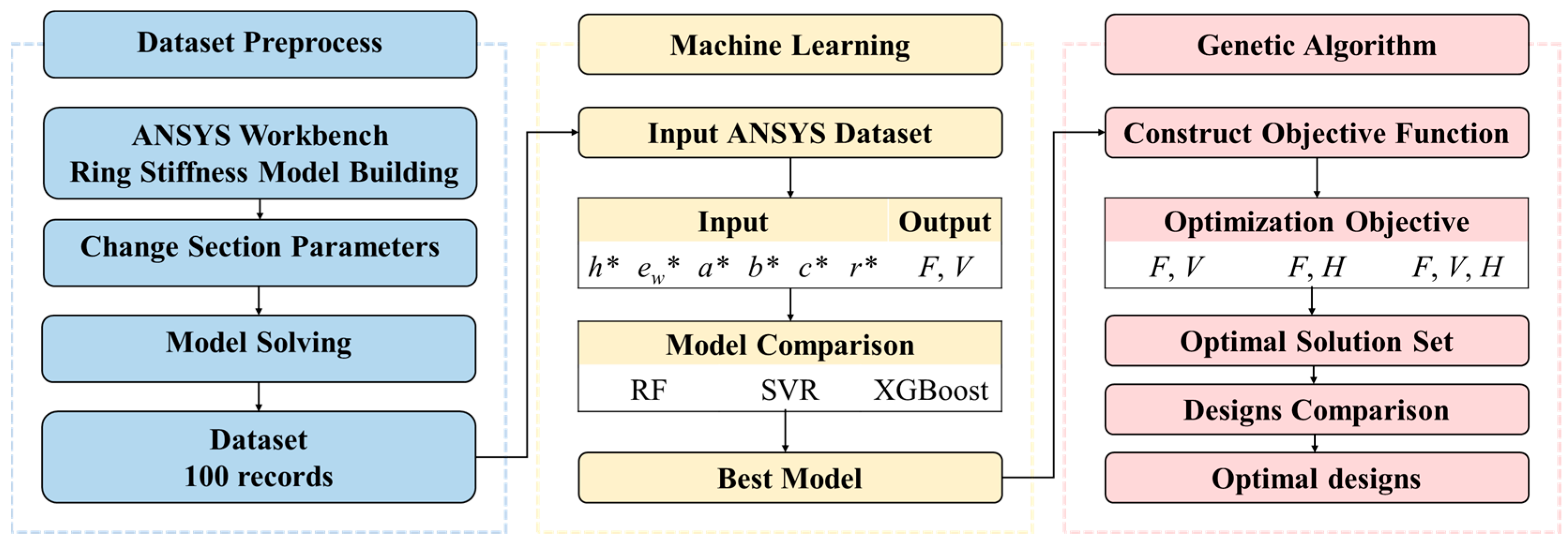
The integration of machine learning (ML) with experimental methods and numerical simulation provides an efficient research pathway for the development of sustainable pipeline rehabilitation technology, significantly enhancing the time efficiency and resource utilization of design optimization [11]. To achieve the sustainable optimization design goals of SWL, this study developed a systematic three-stage research framework. Stage 1: A ring stiffness test model was established and validated, generating high-quality datasets through numerical simulation to support subsequent predictive modeling. Stage 2: Advanced ML algorithms, including Random Forest (RF), Support Vector Regression (SVR), and Extreme Gradient Boosting (XGBoost), were employed to establish high-accuracy predictive models for loading force (F) and V, enabling intelligent prediction of structural performance. Stage 3: A genetic optimization algorithm framework was constructed based on the predictive models, conducting multi-objective optimization with maximized F, minimized V, and minimized H to achieve an optimal balance between structural performance and resource efficiency. This framework not only enables rapid performance prediction for various designs but also delivers optimal configurations for rehabilitation projects, effectively reducing design cycles, lowering testing costs, and enhancing design reliability.

2. Materials and Methods

2.1. Spiral Wound Strip Profile

A spiral wound strip profile was made from PVC using a continuous extrusion process, and the strip was produced by Shanghai Qingyuan Pipe Industry Technology Co., Ltd. in Shanghai, China. The sections of the strip profile are shown in Figure 1a, and the liner formed by a special winding unit is shown in Figure 1b.

The section parameters of the strip profile were dimensionless with the effective width w: a is the height of the T-rib top plate, b is the width of the T-rib top plate, c is the width of the T-rib waist, e_w is the wall thickness of the strip profile, h is the height of T-rib waist, and r is the radius of T-rib top plate. After normalization, the section parameters were a* = a/w, b* = b/w, c* = c/w, e_w* = e_w/w, h* = h/w, and r* = r/w, where * denotes the dimensionless quantity. The initial structural dimension parameters of the strip profile are presented in

Table 1. Initial dimension parameters of the strip profile.

a*	b*	c*	ew*	h*	r*	w/mm
0.03	0.12	0.039	0.03	0.215	0.0060	90

.

A data set containing 100 groups of profile section parameters was obtained using single-factor and orthogonal design.

Table 2. Statistical information of the train-test dataset.

	h*	ew*	a*	b*	c*	r*
count	100	100	100	100	100	100
mean	0.233750	0.029940	0.031550	0.153400	0.030200	0.006060
std	0.028466	0.001406	0.002743	0.058122	0.015506	0.001869
min	0.205000	0.024000	0.030000	0.080000	0.003600	0.001000
25%	0.215000	0.030000	0.030000	0.120000	0.022000	0.006000
50%	0.215000	0.030000	0.030000	0.120000	0.039000	0.006000
75%	0.251250	0.030000	0.032000	0.180000	0.039000	0.006000
max	0.300000	0.035000	0.040000	0.300000	0.050000	0.012000

presents the statistical information of the data, where count represents the total number of data, mean is the average value, std is the standard deviation, min is the minimum value, 25% is the first quartile, 50% is the median, 75% is the third quartile, and max is the maximum value.

2.2. Ring Stiffness Test Model

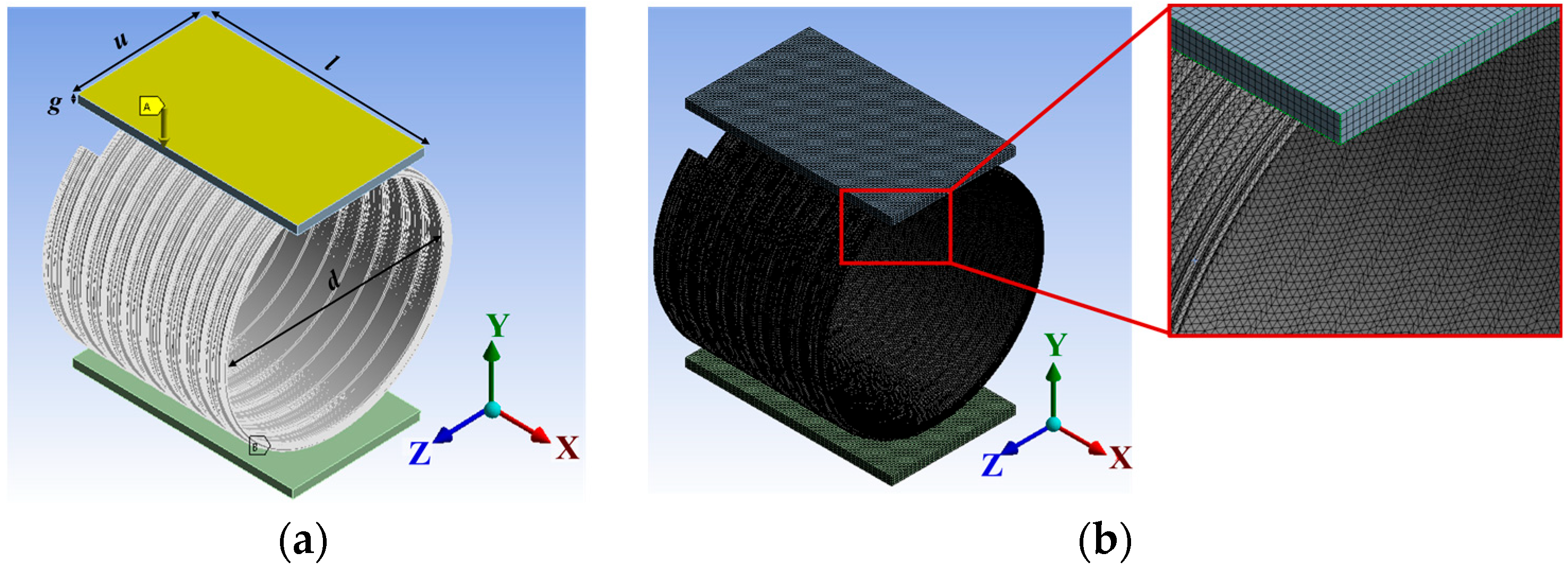
The ring stiffness test model was established using the static structure analysis module in ANSYS finite element analysis software (version 2021 R2, developed by ANSYS, Inc., USA). The inner diameter of the SWL liner was set to d = 1000 mm, the top plate size was l = 1000 mm, u = 600 mm, and g = 40 mm. In the finite element model, displacement constraints were imposed on the top plate. Specifically, in the X and Z directions, the value was set to “0 mm”, while in the Y direction, it was set to “−30 mm”; the lower plate was set as a Fixed Support. The loading method used was displacement loading, causing the top plate to move downward by 30 mm (3% of the inner diameter). The finite element model of the S_p of the SWL liner is shown in Figure 2a. The downward arrow shows a vertical load applied to the top plate. “A” and “B” are software-assigned surface labels.10-node tetrahedral elements were used for the SWL liner, and 20-node hexahedral elements were used for the top and lower plates. The mesh size was set to 10 mm, with a total number of units of 1.1 × 10⁶ and a number of nodes of 2.2 × 10⁶. The mesh division is shown in Figure 2b.

The SWL liner was made of PVC (rigid) from the ANSYS Workbench material library. The elastic modulus E was set to 2500 MPa, a value obtained through tensile testing conducted by the standard GB/T 1040.1-2018 [12]. Tests were performed using a universal testing machine at a speed of 1 mm/min. This value represents the mean of five replicate specimens. These results comply with the elastic modulus requirements specified in standard GB/T 41666.7-2024 [13]. The Poisson’s ratio was set to 0.38, as specified in CJJ/T 210-2014 [14]. Based on von Mises’ constitutive model, the F was obtained by solving the model, and the simulated S_p was calculated by the ring stiffness test formula according to standard ISO 9969-2016 [15], as shown in Equation (1).

$$S_p=\left(0.0186+0.025{\displaystyle \frac{y_F}{d}}\right)\left({\displaystyle \frac{F}{L{y}_F}}\right)\times {10}^6$$

(1)

where $S_p$ is the ring stiffness of the liner, kN/m²; $y_F$ is the deformation relative to the liner 3.0% deformation, mm; d is the inner diameter of the liner, mm; F is the loading force relative to 3.0% deformation of the liner, kN; L is the length of the sample, mm.

2.3. Finite Element Model Validation

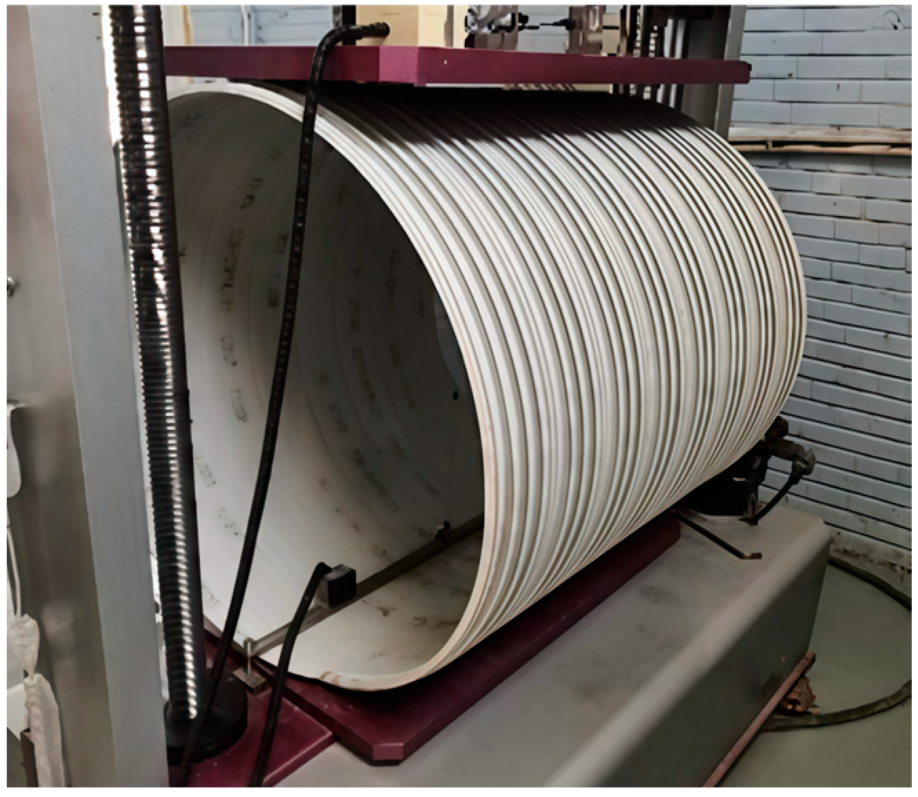
This study conducted a ring stiffness test on a DN1000 SWL liner. The structural dimensions of the pipe section were consistent with the finite element model, and the test setup is illustrated in Figure 3. The experimental measurement yielded a $S_p$ of 0.62 kN/m², while the simulation result was 0.61 kN/m². By comparing the experimental results, a relative error of 1.61% was calculated, thereby validating the reliability of the finite element modeling methodology.

3. Prediction Model

Firstly, ANSYS simulation was used to establish the ring stiffness test model, solve the F of different structures, and obtain the dataset. Then, ML was used to accurately predict the F and V. Finally, multi-objective optimization was achieved through a genetic algorithm, as shown in Figure 4. This chapter mainly introduced the ML prediction algorithm, prediction process, and model evaluation. The datasets used in this study are provided in Appendix A.

3.1. Model Algorithm

To carry out multi-objective optimization design of liner structure, ML models for F and V of the liner were established using RF, SVR, and XGBoost models. The effects of these models were compared, and the best models were selected.

RF is an ensemble learning model based on decision trees. By creating multiple decision trees, each tree in the forest is trained independently, which makes it a parallel and scalable algorithm to average the prediction results of these trees to get the final prediction result [16].

SVR is a nonlinear regression prediction method based on the support vector machine (SVM) model, which can effectively solve the modeling problem of high-dimensional data under limited sample conditions, and has the advantages of strong generalization ability and dimensionality insensitive [17]. The objective function is shown in Equation (2):

$$f\left(x\right)=\underset{\omega ,b,{\delta }_i}{\min }\left[{\displaystyle \frac{1}{2}}{\omega }^2+C\sum _{i=1}^n{\delta }_i\right]$$

(2)

where x represents the input data, ω is the weight vector, b is the biased term, δ_i is the relaxation variable, C is the regularization parameter, and n is the number of samples.

XGBoost model is an ML algorithm for classification and regression problems. Instead of averaging a single tree, the model constructs a series of sequential decision trees using prediction errors or resists from previous tree models [18,19]. The objective function is shown in Equation (3):

$$f\left(x\right)=\sum _{i=1}^{n}l\left(y_i,{\widehat{y}}_i\right)+\sum _{j=1}^k\Omega \left(f_j\right)$$

(3)

where $l\left(y_i,{\widehat{y}}_i\right)$ is the loss between the actual value ($y_i$) and the predicted value (${\widehat{y}}_i$) of sample i, $\Omega \left(f_j\right)$ is the complexity of the j decision tree, and k is the number of trees.

Several different evaluation indicators commonly used in the literature [20,21] were considered in this study.

R squared (R²), also known as the coefficient of determination, is expressed as Equation (4):

$$R^2=1-{\displaystyle \frac{\sum _{i=1}^n{\left(y_i-{\widehat{y}}_i\right)}^2}{\sum _{i=1}^n{\left(y_i-\overline{y}\right)}^2}}$$

(4)

where $\overline{y}$ is the mean of the actual values.

Mean absolute error (MAE) is the absolute value of the difference between the actual value and the predicted value, calculated as Equation (5):

$$MAE={\displaystyle \frac{1}{n}}\sum _{i=1}^n\left|y_i-{\widehat{y}}_i\right|$$

(5)

The mean square error (MSE) is the average of the squared difference between the actual value and the predicted value. It is always a positive value and decreases as the error approaches zero, calculated as Equation (6):

$$MSE={\displaystyle \frac{1}{n}}\sum _{i=1}^n{\left(y_i-{\widehat{y}}_i\right)}^2$$

(6)

To compare the prediction accuracy of the models, the influence of each input on the model prediction process is determined. SHAP values evaluate the importance of different types of inputs to the model [22] as shown in Equation (7):

$$mean SHAP={\sum }_{i=1}^n\phi \left(x^{\left(i\right)}\right)/N_i$$

(7)

3.2. Prediction Model of Ring Stiffness

In this study, RF, SVR, and XGBoost models were used to predict the F in the ring stiffness test with varying section parameters. Six parameters were selected as inputs, namely a*, e_w*, h*, b*, c*, and r*, and F was taken as the output of the model. The train_test_split module was used to separate the data, and it was randomly divided into 70% of the train data and 30% of the test data. All input features were standardized. Specifically, the mean and standard deviation of each feature were computed exclusively on the training set. All ML models were trained using the train dataset and tested using the test dataset to determine their accuracy. To further verify the generalization ability of the model, 5-fold cross-validation (CV) was performed only on the training set, and a fixed random seed of 42 was set. The grid search method [23] was applied to adjust the hyperparameters to improve its accuracy. The candidate hyperparameters were evaluated based on the average validation performance, and the optimal combination was selected.

Table 3. The operational parameters of ring stiffness prediction models.

Algorithm	Hyperparameter	Search Range	Optimal Value
RF	N estimators	(10, 50, 100, 200)	100
	Max depth	(5,10, 20, 30)	10
	Min samples leaf	(1,2, 5, 10)	1
	Min samples split	(1, 2, 4)	2
	bootstrap	(True, False)	True
SVR	Kernel	-	Linear
	C	(0.1, 1, 10, 100, 200)	10
	epsilon	(0.01, 0.05, 0.1, 1, 2)	0.1
XGBoost	N estimators	(100, 200, 300, 400)	300
	Max depth	(1, 2, 3, 4)	2
	Learning rate	(0.01, 0.1, 0.2)	0.2

lists the hyperparameters used in the ring stiffness prediction model.

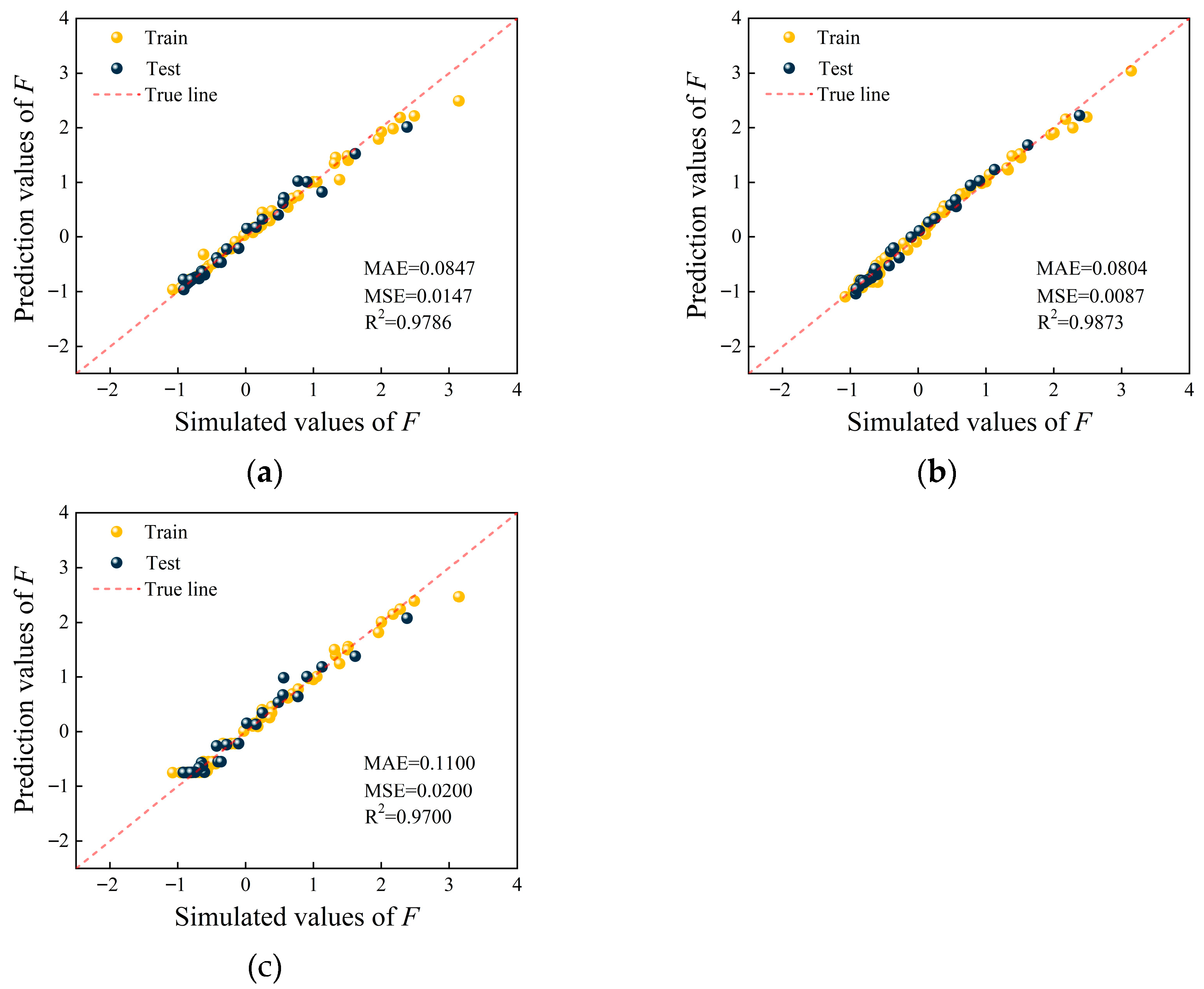
Figure 5 shows the train and test regression graphs for RF, SVR, and XGBoost models, with the SVR model demonstrating the best performance. According to the test data, which were not used for training, the SVR model achieved the highest R² of 0.9873, the lowest MAE of 0.0804, and the lowest MSE of 0.0087.

In general, it is not sufficient to check an ML model against a single metric in a performance evaluation, and

Table 4. The evaluation metrics for the train and test sets of different models predicting F.

Model	R2_train	MSE_train	MAE_train	R2_test	MSE_test	MAE_test
RF	0.9865	0.0135	0.0602	0.9786	0.0147	0.0847
SVR	0.9983	0.0017	0.0386	0.9873	0.0087	0.0804
XGBoost	0.9859	0.0141	0.0727	0.9700	0.0200	0.1100

compares ML models against various evaluation metrics. Table 4 indicates that the SVR model performed best in both the train and test datasets, followed by the RF and XGBoost. All three models achieved an R² greater than 0.98 during training. During training, SVR achieved the highest accuracy at 0.9983, followed by RF at 0.9865, and XGBoost at 0.9859. In the test dataset, which was not used for training, SVR achieved the highest accuracy of 0.9873, RF achieved 0.9786, and XGBoost achieved 0.9700, with none of the three models showing overfitting.

3.3. Prediction Model of Material Consumption

In this study, RF, SVR, and XGBoost models were also used to predict the V under different section parameter variations. 6 parameters were selected as inputs, including a*, e_w*, h*, b*, c*, and r*, and V was selected as the output of the model. The train_test_split module was used to separate the train data from the test data, and was randomly divided into 70% of the train data and 30% of the test data. All input features were standardized. Specifically, the mean and standard deviation of each feature were computed exclusively on the training set. All ML models were trained using the train dataset and tested using the test dataset to determine their accuracy. To further verify the generalization ability of the model, 5-fold cross-validation (CV) was performed only on the training set, and a fixed random seed of 42 was set. The grid search method [23] was applied to adjust the hyperparameters to improve its accuracy. The candidate hyperparameters were evaluated based on the average validation performance, and the optimal combination was selected.

Table 5. The operational parameters of V prediction models.

Algorithm	Hyperparameter	Search Range	Value
RF	N estimators	(50, 100, 150, 200)	100
	Max depth	(20, 30, 40, 50)	30
	Min samples leaf	(1,2, 5, 10)	1
	Min samples split	(1, 2, 4)	2
	bootstrap	(True, False)	True
SVR	Kernel	-	Rbf
	C	(1, 10, 50, 100)	10
	epsilon	(0.01, 0.05, 0.1, 0.2)	0.05
	gamma	(0.1, 0.2, 0.5)	0.2
XGBoost	N estimators	(200, 300, 400, 500)	300
	Max depth	(1, 2, 3, 4)	2
	Learning rate	(0.01, 0.1, 0.2,0.3)	0.3

lists the hyperparameters used in the V prediction model.

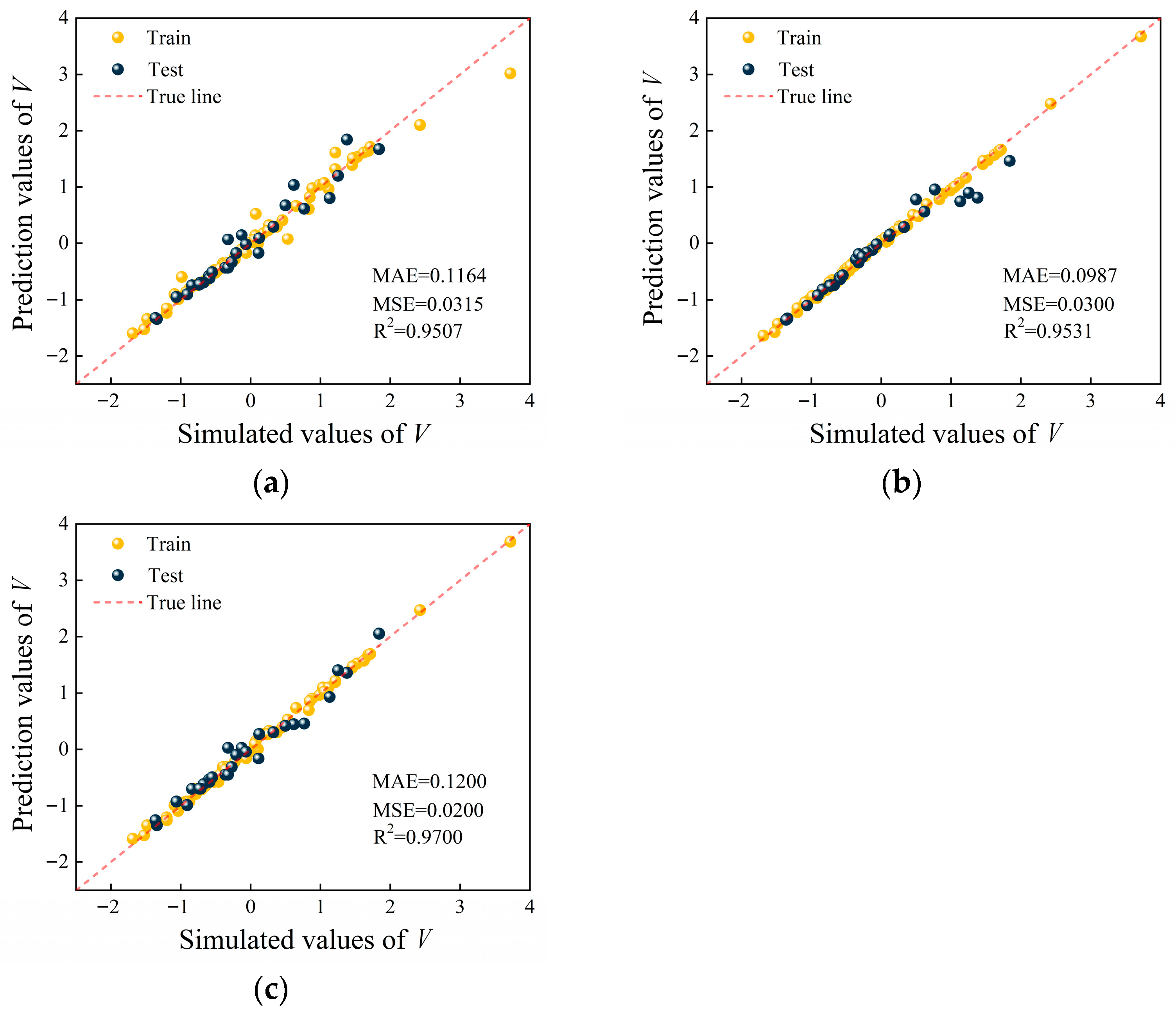
Figure 6 shows the training and testing regression graphs for RF, SVR, and XGBoost models. The XGBoost model exhibited the highest performance. According to the test data, which was not used for training, the test set R² was as high as 0.9700, MAE as low as 0.0200, and MSE as low as 0.1200.

Table 6. The evaluation metrics for the train and test sets of different models predicting V.

Model	R2_train	MSE_train	MAE_train	R2_test	MSE_test	MAE_test
RF	0.9777	0.0223	0.0767	0.9507	0.0315	0.1164
SVR	0.9907	0.0093	0.0783	0.9531	0.0300	0.0987
XGBoost	0.9974	0.0026	0.0369	0.9700	0.0200	0.1200

compares the ML models using different evaluation indicators. The XGBoost model shows the best performance in both the training and test data sets, making it the preferred choice for predicting V.

4. Multi-Objective Optimization of the Structure Size of Spiral Wound Strip Profile

A genetic algorithm is a computational model based on population evolution. It facilitates information exchange and survival of the fittest through reproduction, variation, and competition among individuals in the population to gradually approach the optimal solution [24]. A Non-dominated sorting genetic algorithm (NSGA) is a common method to solve multi-objective optimization problems. The NSGA-Ⅱ optimization algorithm, an improved version of NSGA, has the advantages of good exploration, higher optimization efficiency, and clearer solution set frontier [25,26]. The NSGA-II optimization algorithm of the genetic algorithm was selected to carry out the multi-objective optimization design of the liner.

4.1. Optimal Design

$S_p$ is a crucial index for evaluating the mechanical properties of the liner. Under fixed test conditions (specifically a pipe inner diameter of 1000 mm and sample length of 1000 mm), $S_p$ and F are interconvertible through Equation (1). Consequently, F was adopted as the optimization objective in this study due to its direct experimental and simulation measurability. F values were subsequently converted to $S_p$ during post-processing to ensure this core engineering parameter was explicitly presented in final results.

At the same time, pipeline design must control both V and H. Since the SWL method involves inserting liners into host pipes, the inner diameter of the repaired pipeline equals the original inner diameter minus 2H. Therefore, the smaller the H, the larger the inner diameter of the repaired pipeline will be. The cross-sectional area of the pipeline will be larger.

4.1.1. Multi-Objective Optimization of F and V

Multi-objective optimization was carried out with maximum F and minimum V as two objectives. To obtain the Pareto optimal frontier more intuitively in the figure, the multi-objective column of F maximization was treated as −F minimization, as shown in Equation (8).

$$\left\{\begin{array}{c}tofind:a^{*},b^{*},c^{*},e_w^{*},h^{*},r^{*}\\ \hspace{1em}min:\left[-F,V\right]\end{array}\right.$$

(8)

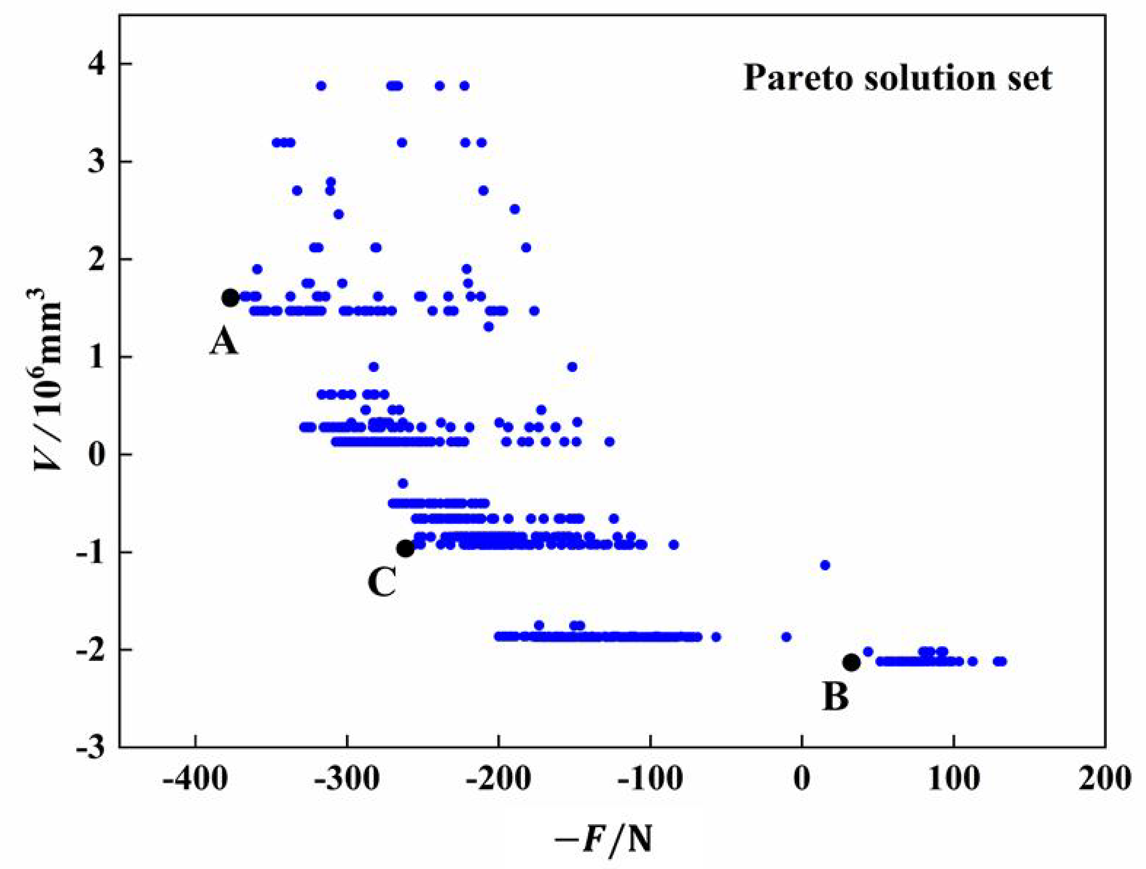
Setting the initial optimal population size to 100 and genetic algebra to 200, 1284 Pareto optimal solution sets were calculated based on the NSGA-II optimization algorithm, and the resulting Pareto optimal solution sets are shown in Figure 7.

As seen in Figure 7, point A in the Pareto optimization solution set represents the section design when the negative value −F is minimized in single objective optimization, resulting in the highest liner S_p. Point B represents the design with the minimum V in single objective optimization, resulting in the smallest volume. Point C represents the optimal section design considering both F and V. The section parameter design scheme represented by the three points is shown in

Table 7. Typical designs of section parameters.

	h*	ew*	a*	b*	c*	r*	Description
A	0.30	0.034	0.039	0.11	0.051	0.0010	F is the maximum single target.
B	0.22	0.030	0.031	0.12	0.038	0.0067	V is the minimum single target.
C	0.24	0.030	0.039	0.14	0.051	0.0010	Weigh multiple goals for F and V.

.

4.1.2. Multi-Objective Optimization of F and H

Multi-objective optimization was carried out with maximum F and minimum H as the objectives. To obtain the Pareto optimal frontier more intuitively, the multi-objective column of F maximization was transformed into minimizing −F, as shown in Equation (9).

$$\left\{\begin{array}{c}tofind:a^{*},b^{*},c^{*},e_w^{*},h^{*},r^{*}\\ \hspace{1em}min:\left[-F,H\right]\end{array}\right.$$

(9)

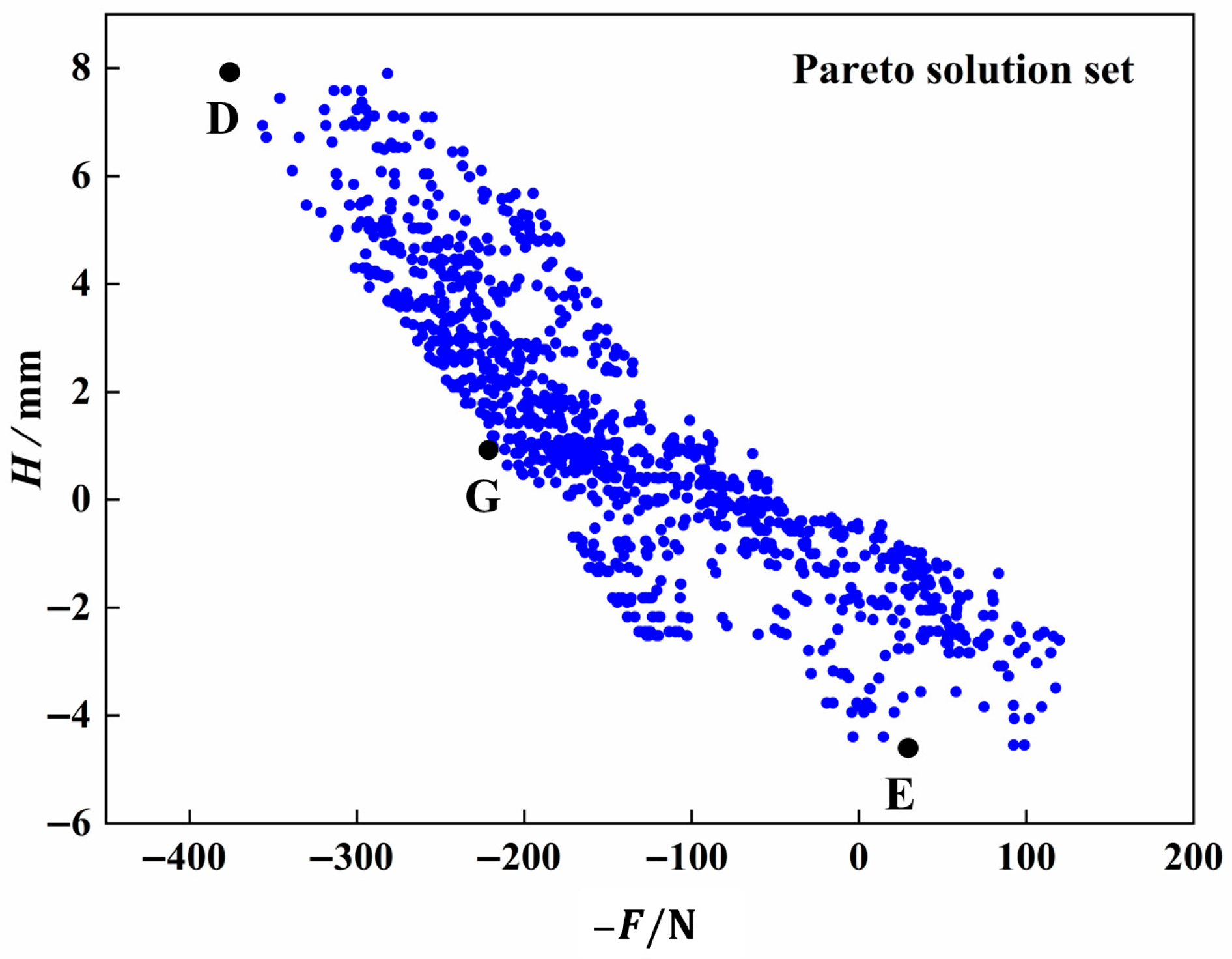
Setting the initial optimal population size to 100 and genetic algebra to 200, 1972 Pareto optimal solution sets were calculated based on the NSGA-II optimization algorithm, and the resulting Pareto optimal solution sets are shown in Figure 8.

As can be seen from Figure 8, in the Pareto optimization solution set, point D represents the section design when the negative value −F is the minimum of single objective optimization, and the liner S_p is the highest at this time. Point E represents the design under the optimization of a single optimization objective with minimum H, and the volume is the smallest at this time. Point G represents the optimal design of the section when the two objectives of F and V are considered. The section parameter design scheme represented by the three points is shown in

Table 8. Typical designs of section parameters.

	h*	ew*	a*	b*	c*	r*	Description
D	0.29	0.034	0.038	0.30	0.049	0.0027	F is the maximum single target.
E	0.21	0.024	0.033	0.15	0.051	0.0022	H is the minimum single target.
G	0.22	0.028	0.039	0.30	0.051	0.0010	Weigh multiple goals for F and H.

.

4.1.3. Multi-Objective Optimization of F, V, and H

Multi-objective optimization was carried out by taking the maximum F, the minimum V and the minimum H of the strip profile in the ring stiffness test of the liner as three optimization objectives. To obtain the Pareto optimal frontier more intuitively in the figure, the maximization of F was treated as the minimization of −F, and the multi-objective column is shown in Equation (10).

$$\left\{\begin{array}{c}tofind\mathit{:}{a}^{*},b^{*},c^{*},e_w^{*},h^{*},r^{*}\\ \hspace{1em}min:\left[-F,V,H\right]\end{array}\right.$$

(10)

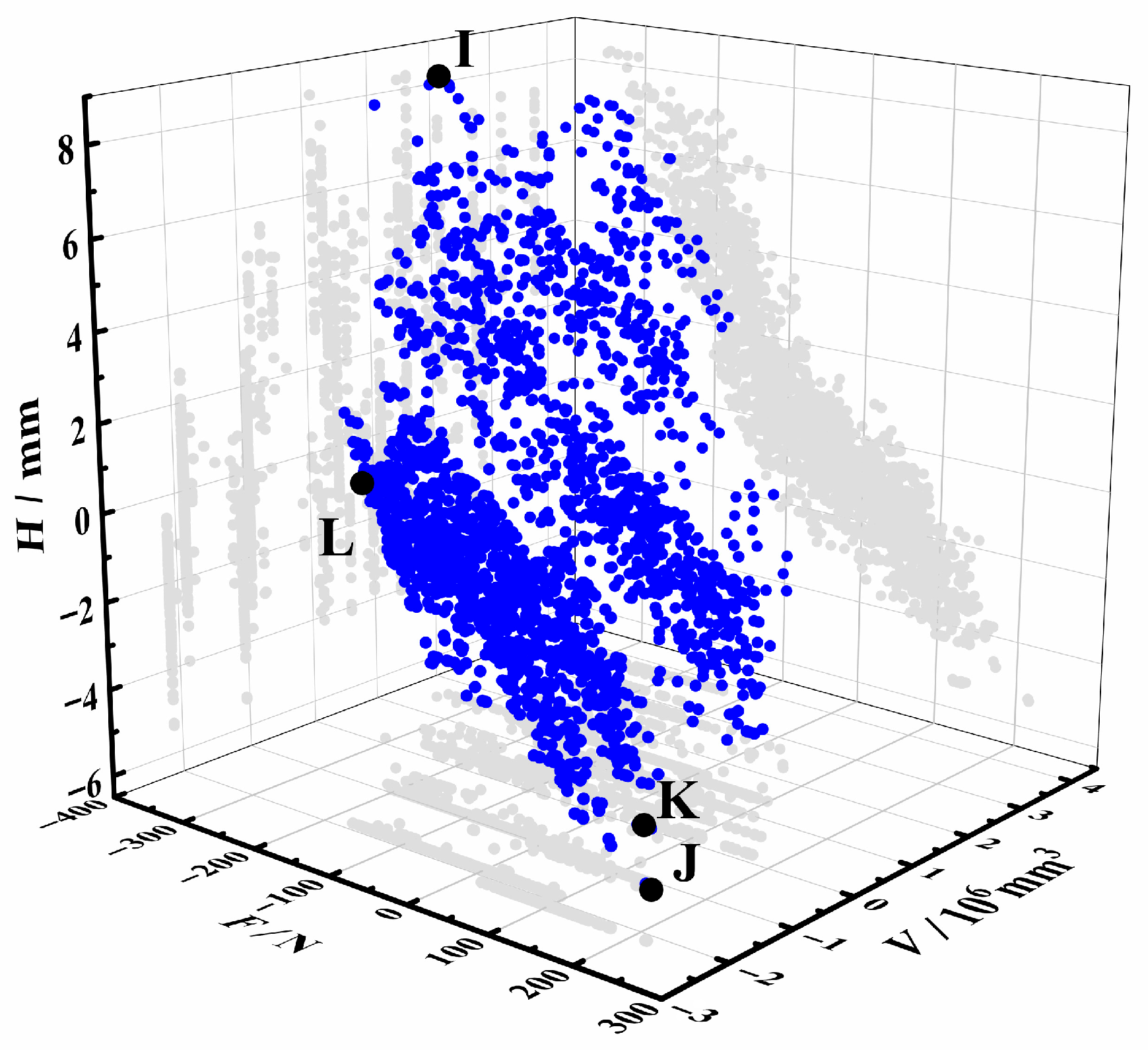
With the initial optimal population size set to 100 and genetic algebra set to 200, 3936 Pareto optimal solution sets were calculated based on the NSGA-Ⅱ optimization algorithm, and the resulting Pareto optimal solution sets are shown in Figure 9.

As can be seen from Figure 9, in the Pareto optimization solution set, point I represents the section design when the negative value −F is the minimum of single objective optimization, and the liner S_p is the highest at this time. Point J represents the design under the optimization of a single optimization objective with minimum V, and the volume is the smallest at this time. Point K represents the design when the H minimum single optimization objective is optimized, and the strip section height is the minimum at this time. Point L represents the optimal design of the section when considering the three objectives of F, V, and H. The section parameter design scheme represented by the four points is shown in

Table 9. Typical designs of section parameters.

	h*	ew*	a*	b*	c*	r*	Description
I	0.30	0.034	0.039	0.13	0.044	0.0015	F is the maximum single target.
J	0.21	0.024	0.030	0.11	0.030	0.0088	V is the minimum single target.
K	0.21	0.024	0.030	0.11	0.047	0.0010	H is the minimum single target.
L	0.22	0.028	0.039	0.13	0.039	0.0012	Weigh multiple goals for F, V, and H.

.

4.2. Optimization Result

The above 10 design schemes were simulated by the finite element method to compare the improvement effect. The calculation results are shown in

Table 10. Typical designs of section parameters.

	F/N	V/106 mm3	H/mm	Sp/(kN/m2)	The Increase Ratio of Sp/%	The Increase Ratio of V/%
A	2803.9	22.9842	33.57	1.8085	137.98	25.31
B	1256.9	18.3834	25.29	0.8107	6.68	0.23
C	1904.9	21.1097	27.81	1.2287	61.68	15.09
D	3893.9	25.8825	32.58	2.5116	230.50	41.11
E	1173.8	18.6794	24.03	1.2605	6.99	1.84
G	2233.9	23.1432	25.83	1.4409	89.60	26.18
I	2966.3	22.3476	33.57	1.9132	151.77	27.29
J	0931.2	15.7222	23.76	0.6006	−20.96	−14.28
K	1054.0	17.4793	23.76	0.6798	−10.54	−4.70
L	1466.4	18.6760	25.83	0.9458	24.46	1.82

.

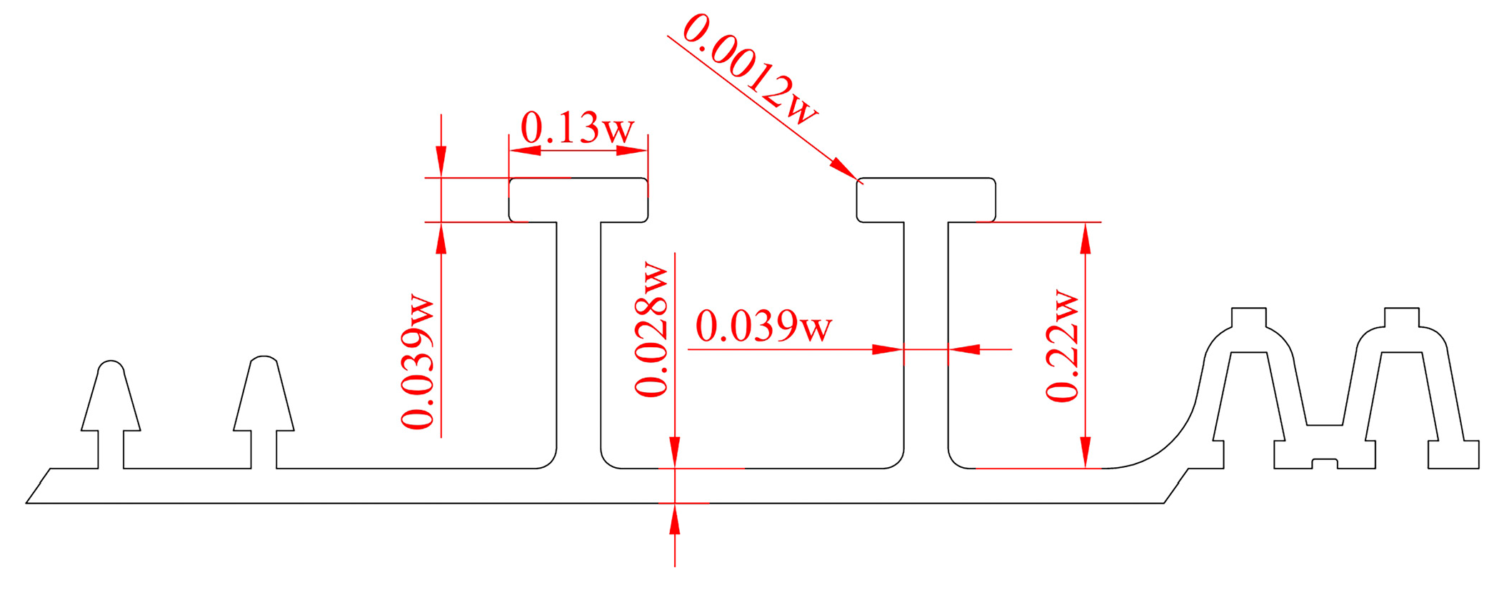
Point L is the selected multi-objective optimization scheme, where h* = 0.22w, e_w* = 0.028w, a* = 0.039w, b* = 0.13w, c* = 0.039w, and r* = 0.0012w. The section of the optimized profile is shown in Figure 10. The S_p of the optimized liner is increased by 24.46%, and the V is only increased by 1.82%.

5. Parameter Analysis

5.1. Single-Factor Experimental Analysis

By controlling a single parameter, the influences of a*, b*, c*, e_w*, h*, and r* on the F and the V were studied. A total of 75 sets of S_p simulation were carried out; the parameters of the section were fitted with the data of F and V, and the fitting formula was obtained, as shown in Figure 11.

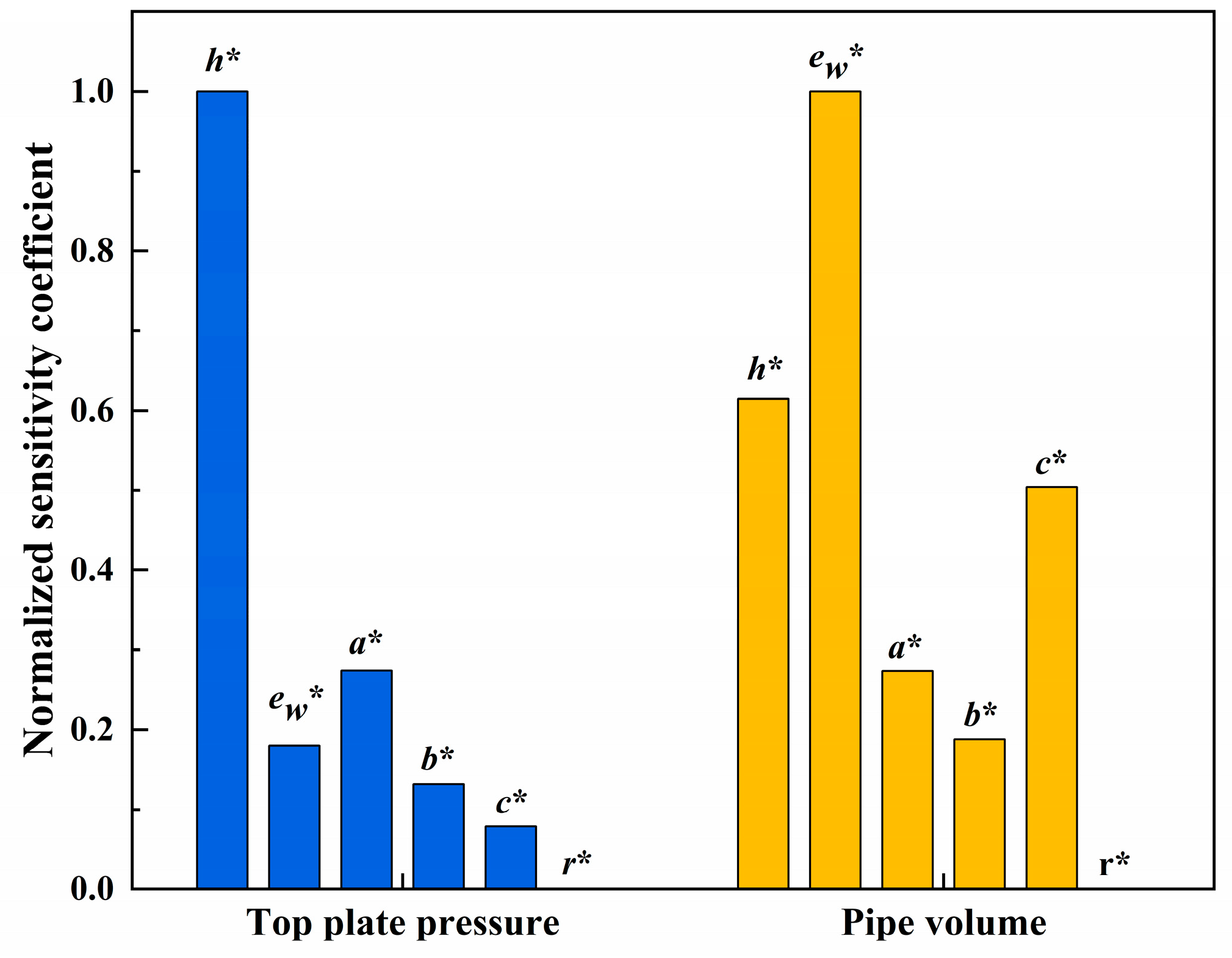
The sensitivity coefficient is defined as the ratio of the degree of sensitive factors to the change degree of the evaluation indicators [27]. By comparing the sensitivity coefficient of different parameters, the influence degree of each parameter on the F and V of the profile was determined. The sensitivity coefficient is expressed by Equation (11).

$$\beta =∆Y/∆X$$

(11)

where β is the sensitivity coefficient of sensitive factor Q; ∆Y is the rate of change of the evaluation index, %; ∆X is the rate of change of the sensitive factor, %.

Figure 12 shows the sensitivity analysis of F and V on 6 parameters. Absolute values of sensitivity coefficients are compared, and max-min normalization is carried out. The results show that the sensitivity coefficients of the F to sensitive factors are as follows: h*, a*, e_w*, b*, c*, and r*, among which the F value has the highest sensitivity to h* and the lowest sensitivity to r*. The order of sensitivity coefficients of V to sensitive factors is: e_w*, h*, c*, a*, b*, r*, among which the sensitivity to e_w* is the highest, and the sensitivity to r* is the lowest.

5.2. Orthogonal Experimental Analysis

In the study, an orthogonal experimental design was carried out for cross-section parameters, and 6 factors and 5 levels of the test scheme were selected, as shown in

Table 11. Factors and levels in the orthogonal experiment.

Level	h*	ew*	a*	b*	c*	r*
1	0.22	0.028	0.030	0.14	0.036	0.002
2	0.24	0.029	0.032	0.18	0.038	0.004
3	0.26	0.03	0.034	0.22	0.040	0.006
4	0.28	0.031	0.036	0.26	0.042	0.008
5	0.30	0.032	0.038	0.30	0.044	0.010

.

ANSYS Workbench software was used to analyze 25 different ring stiffness models of the SWL liner, and the simulation results are shown in

Table 12. Results of the orthogonal experiment.

Level	h*	ew*	a*	b*	c*	r*	F/N	Sp/(kN/m2)
1	0.22	0.028	0.030	0.14	0.036	0.002	1268.2	0.82
2	0.22	0.029	0.034	0.26	0.044	0.004	1895.2	1.22
3	0.22	0.030	0.038	0.18	0.042	0.006	1708.3	1.10
4	0.22	0.031	0.032	0.30	0.040	0.008	1976.2	1.27
5	0.22	0.032	0.036	0.22	0.038	0.010	1841.3	1.19
6	0.24	0.028	0.038	0.26	0.040	0.010	2261.9	1.46
7	0.24	0.029	0.032	0.18	0.038	0.002	1760.6	1.14
8	0.24	0.030	0.036	0.30	0.036	0.004	2409.4	1.55
9	0.24	0.031	0.030	0.22	0.044	0.006	1940.8	1.25
10	0.24	0.032	0.034	0.14	0.042	0.008	1724.1	1.11
11	0.26	0.028	0.036	0.18	0.044	0.008	2189.6	1.41
12	0.26	0.029	0.030	0.30	0.042	0.010	2475.5	1.60
13	0.26	0.030	0.034	0.22	0.040	0.002	2366.9	1.53
14	0.26	0.031	0.038	0.14	0.038	0.004	2060.4	1.33
15	0.26	0.032	0.032	0.26	0.036	0.006	2482.0	1.60
16	0.28	0.028	0.034	0.30	0.038	0.006	2975.2	1.92
17	0.28	0.029	0.038	0.22	0.036	0.008	2760.6	1.78
18	0.28	0.030	0.032	0.14	0.044	0.010	2154.3	1.39
19	0.28	0.031	0.036	0.26	0.042	0.002	2858.4	1.84
20	0.28	0.032	0.030	0.18	0.040	0.004	2376.3	1.53
21	0.30	0.028	0.032	0.22	0.042	0.004	2918.1	1.88
22	0.30	0.029	0.036	0.14	0.040	0.006	2541.0	1.64
23	0.30	0.030	0.030	0.26	0.038	0.008	3036.6	1.96
24	0.30	0.031	0.034	0.18	0.036	0.010	2735.8	1.76
25	0.30	0.032	0.038	0.30	0.044	0.002	3408.0	2.20
Range	0.7676	0.0514	0.1421	0.4510	0.0209	0.0282

.

According to the range results in Table 12, it could be concluded that in the orthogonal test, the primary and secondary order of the influencing factors is h* > b* > a* > r* > c* > e_w*; that is, the height of the T-rib has the greatest influence on the F, followed by the width and height of the roof, which is consistent with the sensitivity analysis results. The wall thickness of the profile, the circle angle of the top plate, and the width of the T-rib waist have little influence on the results.

5.3. SHAP Analysis

SHAP analysis is a method used to interpret the predictions of ML models by quantifying the importance of features by calculating the contribution of each input feature to the model predictions. In SHAP analysis, the higher the input features are on the axis, the more important they are to the model. The importance analysis results of SHAP are shown in Figure 13, and the priority order of the influence of section parameters on F and V is obtained. SHAP analysis results show that, according to the influence of different design parameters on the F, the order from high to low is h*, b*, a*, c*, e_w *, and r*. According to the influence of different design parameters on the V, the order from high to low is b*, h*, a*, e_w *, c*, and r*.

5.4. Analysis of Result Differences

This study employed SHAP analysis, orthogonal experimentation, and sensitivity analysis to evaluate feature importance for F. The SHAP analysis is based on the Shapley value theory in game theory. It quantifies the marginal contribution of each feature to model predictions and explains the importance of the features. Orthogonal experimentation designs a multi-factor orthogonal matrix to focus on the main parameter effects, making it suitable for rapid parameter screening in resource-constrained scenarios. Sensitivity analysis evaluates how input parameter variations contribute to output uncertainty, quantifying global parameter sensitivity.

The SHAP analysis is based on 100 data points in this study, covering a wider feature space. The resultant parameter importance ranking (h* > b* > a* > c* > e_w * > r*) has high credibility. Orthogonal experimentation employed a 25-set design matrix. Although the sample size is small, the ranking of main effects (h* > b* > a* > r* > c* > e_w *) is highly consistent with the SHAP analysis results in the core parameters (h*, b*, a*). The sensitivity analysis has a large fluctuation in the ranking of feature importance due to the small sample size and insufficient sample size.

All three methods identified that feature h* has the most significant impact on F. Features b* and a* are ranked in the top three in both SHAP analysis and orthogonal experimentation, confirming them as secondary key parameters. For other parameters (c*, e_w *, and r*), the differences in ranking mainly result from the principles of the methods and the limitations of sample size. Accordingly, this study proposes a hierarchical importance classification: h* as the primary control parameter, b* and a* as secondary optimization targets, and c*, e_w *, and r* as tertiary parameters.

5.5. Stress Analysis

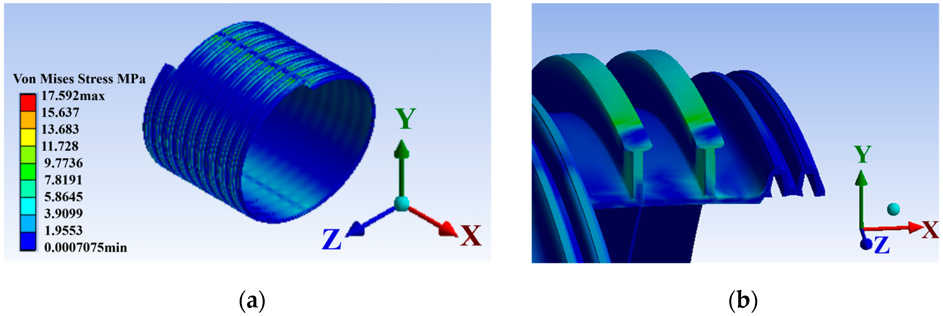
Through finite element simulation analysis, the von Mises stress cloud diagram of the liner is obtained, as shown in Figure 14. It could be seen that the stress distribution of the liner, the maximum stress of the liner is 17.592 MPa, the stress is mainly distributed in the top plate and T-rib waist, and the stress is transferred from the top plate of the strip profile to the bottom plate through the T-rib waist. From a mechanical perspective, the top plate, which directly bears the loads, undergoes deformation under their influence. The resulting deformation-induced stress then propagates along the T-rib waist. This stress transmission and redistribution process plays a vital role in maintaining the overall stability of the liner.

The T-shaped beam structure of the strip profile could be equivalent to an I-beam, in which the top and bottom flanges primarily resist the bending moments under loads, thereby providing good bending resistance. Under loading conditions, the load directly acts on the top plate, which serves as the main load-bearing component.

According to Figure 13, the F is most significantly influenced by the h* and b*. This can be explained by considering the moment of inertia of the cross-section. For analytical simplicity, the strip profile can be idealized as a rectangular cross-section. In such a simplified model, the moment of inertia exhibits a cubic relationship with h* and a linear relationship with b*. Consequently, increasing the values of h* and b* leads to a significant increase in the moment of inertia of the cross-section, which effectively improves the bending performance of the strip profile [28].

The T rib waist mainly bears the effect of shear stress; the increase of the c* value improves the shear resistance of the material, and the stronger its ability to bear the shear stress. Therefore, the change of T rib waist width has a certain influence on the F and V.

In contrast, the F decreases with the increase of the value of r*. The analysis reason is that the decrease of r* reduces the stressed area of the top plate, thus affecting the bearing performance of the liner, but its change has a very weak influence on the F and V.

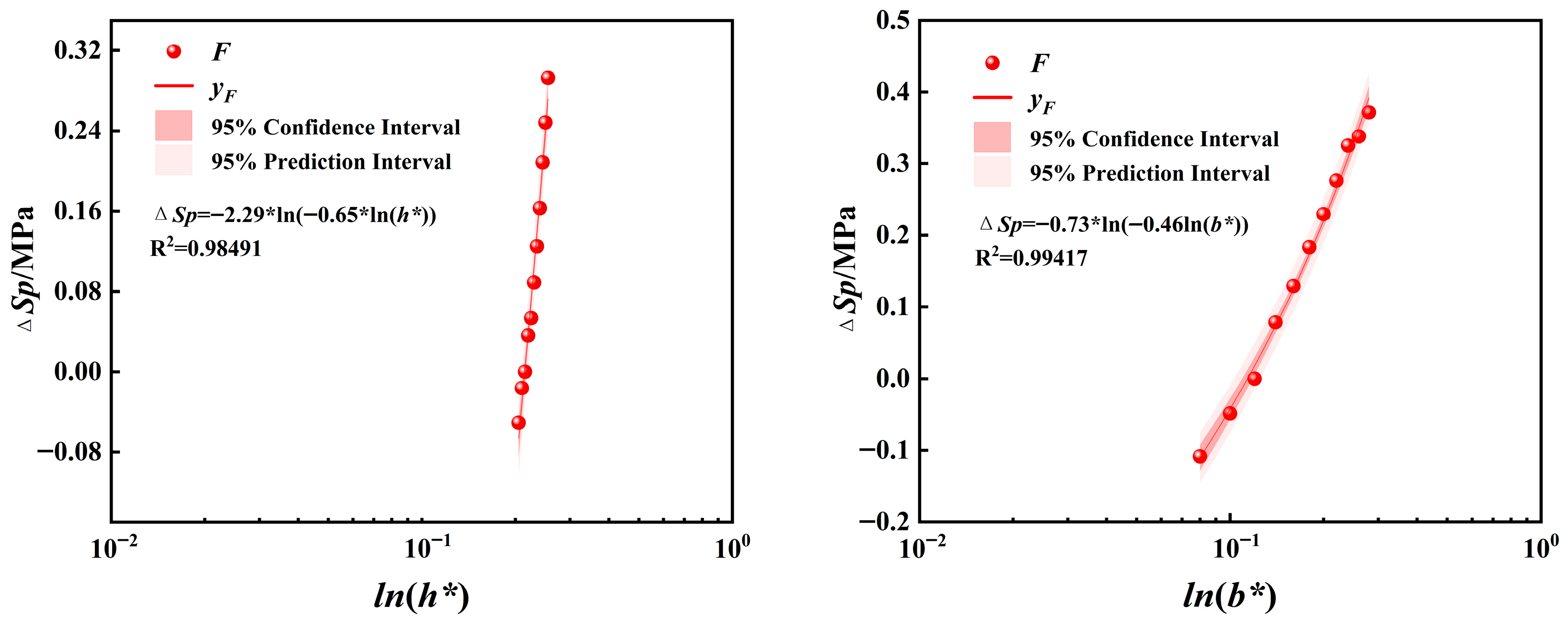
To quantify the relationship between the section parameters h* and b* and S_p increment (ΔS_p), a nonlinear curve fitting method was adopted. The fitting formulas for h* and b* with ΔS_p are provided in Equations (12) and (13). The fitting effect is shown in Figure 15. The ΔS_p prediction formula, derived from Equations (12) and (13), is presented in Equation (14), with an R² value of 0.9874.

$$\left\{\begin{array}{c}{{\Delta S}_p=\mathrm{l}\mathrm{n}\left(f\left(h^{*}\right)\right)}^{-2.29}\\ f\left(h^{*}\right){=\mathrm{l}\mathrm{n}\left(h^{*}\right)}^{-0.65}\end{array}\right.$$

(12)

$$\left\{\begin{array}{c}{\Delta S}_p={\mathrm{l}\mathrm{n}\left(f\left(b^{*}\right)\right)}^{-0.73}\\ f\left(b^{*}\right){=\mathrm{l}\mathrm{n}\left(b^{*}\right)}^{-0.46}\end{array}\right.$$

(13)

$${\mathsf{\Delta }S}_p=-0.071·\mathrm{l}\mathrm{n}\left\{{\left(f\left(h^{*}\right)\right)}^3·\left(f\left(b^{*}\right)\right)\right\}$$

(14)

6. Conclusions

This paper proposes a comprehensive optimization method for SWL liners, achieving synergistic enhancement of environmental benefits and structural performance through a three-stage innovative framework. First, an ANSYS finite element simulation was employed to establish a numerical test model for S_p, generating high-quality datasets through systematic simulation analysis. Second, advanced ML algorithms were utilized to achieve precise predictive modeling of F and V. Finally, a multi-objective optimization solution framework was constructed based on genetic algorithms, obtaining optimal design schemes while balancing structural safety and resource conservation. The key conclusions are as follows:

➀

Based on simulation data, three ML models, RF, XGBoost, and SVR, were established. The SVR model achieved a high accuracy prediction of F (R² = 0.9873), while the XGBoost model excelled in predicting V (R² = 0.9700).

➁

Using the NSGA-II genetic algorithm, multi-objective optimization with objectives of maximizing F, minimizing V, and minimizing H produced the optimal section: h* = 0.22, ew* = 0.028, a* = 0.039, b* = 0.13, c* = 0.039, and r* = 0.0012. The optimized liner S_p increased by 24.46%, and the V only increased by 1.82%.

➂

The parameters h* and b* of the strip profile have the most significant influence on S_p. The relationship between h*, b*, and ΔS_p was quantified through a predictive formula (R² = 0.9874), providing theoretical guidance for optimal design.

References

1. Li, B.; Yu, W.; Xie, Y.E.; Fang, H.Y.; Du, X.M.; Wang, N.N.; Zhai, K.J.; Wang, D.C.; Chen, X.M.; Du, M.R.; et al. Trenchless rehabilitation of sewage pipelines from the perspective of the whole technology chain: A state-of-the-art review. Tunn. Undergr. Space Technol. 2023, 134, 105022. [Google Scholar] [CrossRef]
2. Fang, H.Y.; Li, B.; Wang, F.M.; Wang, Y.K.; Cui, C. The mechanical behaviour of drainage pipeline under traffic load before and after polymer grouting trenchless repairing. Tunn. Undergr. Space Technol. 2018, 74, 185–194. [Google Scholar] [CrossRef]
3. Ma, B.S.; Najafi, M. Development and applications of trenchless technology in China. Tunn. Undergr. Space Technol. 2008, 23, 476–480. [Google Scholar] [CrossRef]
4. Huang, D.; Liu, X.H.; Jiang, S.Z.; Wang, H.C.; Wang, J.Y.; Zhang, Y.K. Current state and future perspectives of sewer networks in urban China. Front. Environ. Sci. Eng. 2018, 12, 2. [Google Scholar] [CrossRef]
5. Ti, Z.S.; Wang, F.Z.; Zhao, Y.H.; Ma, B.S.; Zeng, C.; Liao, B.Y. Theoretical Study on Design of Composite Lining Structure with Rigid-Flexible Combination for Trenchless Pipeline Rehabilitation. Appl. Sci. 2022, 12, 5374. [Google Scholar] [CrossRef]
6. Hu, Y.; Summers, J.; Hiltner, A.; Baer, E. Correlation of fatigue and creep crack growth in poly(vinyl chloride). J. Mater. Sci. 2003, 38, 633–642. [Google Scholar] [CrossRef]
7. Gao, R.; Kuang, T.J.; Meng, X.B.; Huo, B.J. Effects of Ground Fracturing with Horizontal Fracture Plane on Rock Breakage Characteristics and Mine Pressure Control. Rock Mech. Rock Eng. 2021, 54, 3229–3243. [Google Scholar] [CrossRef]
8. Gao, R.; Bai, D.; Yu, B.; Tai, Y.; Meng, X.B.; Zhang, W.Y. Ground fracturing of multi-strata for strong ground pressure control in extra-thick coal seams with hard roofs: Numerical simulation and case study. Eng. Fract. Mech. 2024, 303, 110129. [Google Scholar] [CrossRef]
9. Wang, B.D.; Liu, X.B.; Zhang, H.; Liu, X.; Xu, L.X. A combined experimental and numerical simulation approach for burst pressure analysis of fiber-reinforced thermoplastic pipes. Ocean. Eng. 2021, 236, 109517. [Google Scholar] [CrossRef]
10. Alshboul, O.; Almasabha, G.; Shehadeh, A.; Al Hattamleh, O.; Almuflih, A.S. Optimization of the Structural Performance of Buried Reinforced Concrete Pipelines in Cohesionless Soils. Materials 2022, 15, 4051. [Google Scholar] [CrossRef]
11. Yin, P.B.; Wang, J.J.; He, W.; Wang, S.Q.; Li, X.; Jia, Z. Machine learning-based study on the mechanical properties and embankment settlement prediction model of nickel-iron slag modified soil. Constr. Build. Mater. 2024, 431, 136468. [Google Scholar] [CrossRef]
12. GB/T 1040.1-2018; Standardization Administration of China. Plastics—Determination of Tensile Properties of Plastics—Part 1: General Principles. Standards Press of China: Beijing, China, 2018.
13. GB/T 411666.7-2024; Standardization Administration of China. Plastics Piping Systems for Renovation of Underground Non-pressure Drainage and Sewerage Networks-Part 7: Lining with Spirally-Wound Pipes. Standards Press of China: Beijing, China, 2024.
14. CJJ/T 210-2014; China Urban Water Supply and Sewerage Association. Technical Specification for Trenchless Rehabilitation and Renewal of Urban Sewer Pipeline. China Architecture & Building Press: Beijing, China, 2014.
15. ISO 9969:2016; Thermoplastics Pipes—Determination of Ring Stiffness. International Organization for Standardization: Geneva, Switzerland, 2016.
16. Hu, D.; Hu, Y.J.; Yi, S.; Liang, X.Q.; Li, Y.S.; Yang, X. Surface Settlement Prediction of Rectangular Pipe-Jacking Tunnel Based on the Machine-Learning Algorithm. J. Pipeline Syst. Eng. Pract. 2024, 15, 04023061. [Google Scholar] [CrossRef]
17. Gholami, H.; Shahrooi, S.; Shishesaz, M. Predicting the Burst Pressure of High-Strength Carbon Steel Pipe with Gouge Flaws Using Artificial Neural Network. J. Pipeline Syst. Eng. Pract. 2020, 11, 04020034. [Google Scholar] [CrossRef]
18. Ventriglia, R.M.; Dantas, L.F.; Brandao, B.; Hamacher, S.; Rocha, M.V.B.; David, A.S.; Ribeiro, F.C. Applying Machine Learning to the Fuel Theft Problem on Pipelines. J. Pipeline Syst. Eng. Pract. 2023, 14, 04023011. [Google Scholar] [CrossRef]
19. Rajasekaran, U.; Kothandaraman, M. Comparative Analysis of Machine Learning and Deep Learning Based Water Pipeline Leak Detection Using EDFL Sensor. J. Pipeline Syst. Eng. Pract. 2023, 14, 04023026. [Google Scholar] [CrossRef]
20. Peng, H.Y.; Lu, H.F.; Xu, Z.D.; Wang, Y.J.; Zhang, Z.W. Predicting Solid-Particle Erosion Rate of Pipelines Using Support Vector Machine with Improved Sparrow Search Algorithm. J. Pipeline Syst. Eng. Pract. 2023, 14, 04022077. [Google Scholar] [CrossRef]
21. Shakya, D.; Agarwal, M.; Deshpande, V.; Kumar, B. Estimating Particle Froude Number of Sewer Pipes by Boosting Machine-Learning Models. J. Pipeline Syst. Eng. Pract. 2022, 13, 04022012. [Google Scholar] [CrossRef]
22. Zhang, J.; Li, T.; Yao, Y.Y.; Hu, X.M.; Zuo, Y.P.; Du, H.; Yang, J.M. Optimization of mix proportion and strength prediction of magnesium phosphate cement-based composites based on machine learning. Constr. Build. Mater. 2024, 411, 134738. [Google Scholar] [CrossRef]
23. Ding, Y.J.; Wei, W.; Wang, J.J.; Wang, Y.H.; Shi, Y.X.; Mei, Z.J. Prediction of compressive strength and feature importance analysis of solid waste alkali-activated cementitious materials based on machine learning. Constr. Build. Mater. 2023, 407, 133545. [Google Scholar] [CrossRef]
24. Kakeshpour, M.; Ghazizadeh, M.J.; Hosseini, S.A.; Sharafati, A. Design of District Metered Areas for Existing Water Distribution Networks. J. Pipeline Syst. Eng. Pract. 2024, 15, 04024006. [Google Scholar] [CrossRef]
25. Zhu, Z.H.; Xiao, P.; Kang, A.H.; Kou, C.J.; Chen, J.P. Preparation of biomass composites with high performance and carbon sequestration from waste wood fibers. Constr. Build. Mater. 2023, 404, 133295. [Google Scholar] [CrossRef]
26. Chen, H.Y.; Cao, Y.; Liu, Y.; Qin, Y.W.; Xia, L.Y. Enhancing the durability of concrete in severely cold regions: Mix proportion optimization based on machine learning. Constr. Build. Mater. 2023, 371, 130644. [Google Scholar] [CrossRef]
27. Zhang, M.M.; Fan, X.Y.; Zhang, Q.G.; Yang, B.Z.; Zhao, P.F.; Yao, B.W.; Ran, J.W. Parametric sensitivity study of wellbore stability in transversely isotropic medium based on polyaxial strength criteria. J. Pet. Sci. Eng. 2021, 197, 108078. [Google Scholar] [CrossRef]
28. Zhou, H.L.; Hu, D.M.; Zhang, W.; Gu, B.H.; Sun, B.Z. The transverse impact responses of 3-D braided composite I-beam. Compos. Part A-Appl. Sci. Manuf. 2017, 94, 158–169. [Google Scholar] [CrossRef]
Figure 1. Schematic diagram of SWL liner: (a) strip profile; (b) liner.
Sustainability 17 08109 g001
Figure 2. Ring stiffness test model of SWL liner: (a) Static structural analysis; (b) Meshing.
Sustainability 17 08109 g002
Figure 3. Ring stiffness test.
Sustainability 17 08109 g003
Figure 4. Flow chart of optimization of liner structure.
Sustainability 17 08109 g004
Figure 5. Standardized predictions of F of three ML models: (a) RF; (b) SVR; (c) XGBoost.
Sustainability 17 08109 g005
Figure 6. Standardized predictions of V of three ML models: (a) RF; (b) SVR; (c) XGBoost.
Sustainability 17 08109 g006
Figure 7. Pareto solution for multi-objective optimization of liner F and V.
Sustainability 17 08109 g007
Figure 8. Pareto solution for multi-objective optimization of liner F and H.
Sustainability 17 08109 g008
Figure 9. Pareto solution for multi-objective optimization of liner.
Sustainability 17 08109 g009
Figure 10. Optimized profile section.
Sustainability 17 08109 g010
Figure 11. Influence of section parameters on F and V.
Sustainability 17 08109 g011
Figure 12. Sensitivity analysis of F and V to 6 variables.
Sustainability 17 08109 g012
Figure 13. SHAP analysis:(a) F; (b) V.
Sustainability 17 08109 g013
Figure 14. Stress analysis: (a) Pipe stress distribution; (b) Von Mises stress contour plot.
Sustainability 17 08109 g014
Figure 15. The fitting formula of F with h* and b*.
Sustainability 17 08109 g015