Article

Hybrid Deep Learning Combining Mode Decomposition and Intelligent Optimization for Discharge Forecasting: A Case Study of the Baiquan Karst Spring

1
School of Mathematics and Statistics, North China University of Water Resources and Electric Power, Zhengzhou 450046, China
2
School of Geosciences and Engineering, North China University of Water Resources and Electric Power, Zhengzhou 450046, China
3
Ecological Environment Geo-Service Center of Henan Geological Bureau, Zhengzhou 450000, China
*
Author to whom correspondence should be addressed.
Sustainability 2025, 17(18), 8101; https://doi.org/10.3390/su17188101
Submission received: 3 August 2025 / Revised: 1 September 2025 / Accepted: 1 September 2025 / Published: 9 September 2025

Abstract

Karst springs play a critical strategic role in regional economic and ecological sustainability, yet their spatiotemporal heterogeneity and hydrological complexity pose substantial challenges for flow prediction. This study proposes FMD-mGTO-BiGRU-KAN, a four-stage hybrid deep learning architecture for daily spring flow prediction that integrates multi-feature signal decomposition, meta-heuristic optimization, and interpretable neural network design: constructing an Feature Mode Decomposition (FMD) decomposition layer to mitigate modal aliasing in meteorological signals; employing the improved Gorilla Troops Optimizer (mGTO) optimization algorithm to enable autonomous hyperparameter evolution, overcoming the limitations of traditional grid search; designing a Bidirectional Gated Recurrent Unit (BiGRU) network to capture long-term historical dependencies in spring flow sequences through bidirectional recurrent mechanisms; introducing Kolmogorov–Arnold Networks (KAN) to replace the fully connected layer, and improving the model interpretability through differentiable symbolic operations; Additionally, residual modules and dropout blocks are incorporated to enhance generalization capability, reduce overfitting risks. By integrating multiple deep learning algorithms, this hybrid model leverages their respective strengths to adeptly accommodate intricate meteorological conditions, thereby enhancing its capacity to discern the underlying patterns within complex and dynamic input features. Comparative results against benchmark models (LSTM, GRU, and Transformer) show that the proposed framework achieves 82.47% and 50.15% reductions in MSE and RMSE, respectively, with the NSE increasing by 8.01% to 0.9862. The prediction errors are more tightly distributed, and the proposed model surpasses the benchmark model in overall performance, validating its superiority. The model’s exceptional prediction ability offers a novel high-precision solution for spring flow prediction in complex hydrological systems.

1. Introduction

Karst aquifers, as an important groundwater resource, are widely distributed in karst landforms around the world, especially in China, Europe, and the United States [1,2]. The groundwater systems in these areas usually have complex hydrological characteristics, and the interaction of cracks, fractures, and micropores forms a complex groundwater flow network [3,4,5]. As a visible manifestation of the groundwater system, karst springs serve as a crucial indicator for understanding the system’s dynamics [6]. Moreover, springs play a vital role in supporting ecological, economic, and societal development [7]. Consequently, investigating springs is of paramount importance.
There has been a growing body of research on simulation and prediction techniques for spring discharge in recent years, with widespread applications. Gallegos et al. [8] used MODFLOW-CFP to establish a pipeline flow numerical model and analyzed the impact of karst pipeline structure on the change of spring water flow. Some scholars have proposed that semi-distributed hydrological models exhibit excellent performance in predicting watershed runoff and spring discharge, particularly during high-flow and low-flow periods [9]. Çallı et al. [10] proposed a new preprocessing method SCA routine, based on the KarstMod model, which fully considered the impact of snowmelt on spring water flow and further improved the model representation ability. Models based on physical methods can provide valuable information for understanding the hydrological processes of groundwater environments, but these methods rely on a large amount of observational data on hydrological and geological conditions. To overcome the problem of insufficient data, [11] constructed a simple physical model, DISHMET, that does not require complex parameters and high-precision input data. It is used to reconstruct historical spring flow in the absence of model assumptions. Therefore, it has strong applicability and can be used in spring flow prediction scenarios in different regions. For incomplete time series data, Katsanou et al. [12] improved the Modkarst model [13] in the time dimension, which can process and fill in incomplete data, reduce the impact of missing data on model accuracy, and provide estimates for some key parameters of karst aquifers. Although these improved models help solve the problem of incomplete data, they still rely on a large amount of observational data and detailed basin geological data, and the model calculation is large, making it difficult to adapt to complex or data-deficient areas.
Recently, many scholars have conducted studies to understand the temporal changes in spring discharge by analyzing historical records, which has facilitated forecasting. For example, Farzin et al. [14] combined statistical methods with machine learning methods to explore the differences in groundwater potential prediction using different combination models. Granata et al. [15] used three machine learning models to predict spring flow and concluded that a small amount of spring flow and precipitation data can achieve good prediction results. At present, some studies have begun to apply deep learning methods to spring flow prediction. The study developed a novel integration of decomposition techniques with LSTM, and the findings revealed that the fused model exhibits superior predictive capabilities compared to the individual LSTM model [16,17]. The DWT-WaveNet-LSTM model constructed for spring flow prediction is superior to the single model at all time steps by Zhou et al. [18]. Pölz et al. [19] conducted a comparative analysis and believed that Transformer has a greater advantage in spring flow prediction when the response time is longer. However, due to the complex architecture of models such as Transformer, it is difficult to effectively model local time series features under small sample sizes. Therefore, the GRU model is more suitable for small sample time series prediction tasks [20].
For subsequences with nonlinear and non-stationary properties, direct modeling will affect the robustness and accuracy of the model [21]. Therefore, some studies have tried to use time-frequency analysis methods for noise reduction. For example, Zhou et al. [22,23] applied the DWT and EEMD algorithms to decompose precipitation characteristics, thereby facilitating the capture of overall trends and extraction of valuable information across multiple scales. An et al. (2020) [17] used the decomposition results of SSA and EEMD to build models and compared the effects of different decomposition methods on the model results. The selection of hyperparameters in deep learning algorithms has a significant impact on the model’s effect. The manual tuning of parameters is characterized by significant temporal and equipment costs; hence, the utilization of intelligent optimization algorithms has become increasingly prevalent [24]. Rahbar et al. and Zhang et al. have successfully utilized a genetic algorithm (GA) for hyperparameter optimization in their prediction models and achieved good results. Dodangeh et al. [25] used GA and HS in combination with different models, respectively, and proved that the model performance was significantly improved and the transferability of the model was enhanced after use. The AGTO [26] intelligent optimization algorithm is a multi-faceted improvement on the GTO [27] intelligent algorithm. It enhances global search capabilities, convergence speed, and adaptability, and can better solve complex optimization problems. Hussien et al. [28] found that many fields of research use the AGTO optimization algorithm, which is of great help to their own research. For example, Singh et al. [29] applied it to the field of wind farm market bidding, calculated the optimal bidding strategy, and solved the nonlinear optimization problem. Tayab et al. [30] utilized the AGTO algorithm to fine-tune the hyperparameters of the proposed machine learning and deep learning models, resulting in optimal performance. Although new intelligent optimization algorithms such as AGTO have demonstrated excellent capabilities, they have not yet been widely used in the hydrological field.
This study proposes a long-term transferable hybrid model, FMD-mGTO-BiGRU-KAN, which integrates BiGRU [31] and Kolmogorov—Arnold Networks [32] to capture complex temporal patterns in spring discharge. FMD [33] decomposes nonlinear, non-stationary precipitation data into multiple intrinsic mode functions, enhancing the model’s adaptability to different frequency components. The decomposed precipitation components and mean temperature serve as inputs. The integrated architecture incorporates convolutional feature extraction and residual connections to enhance representational capacity, while employing dropout regularization and L2-norm constraints to mitigate overfitting and improve training stability/efficiency. Advanced intelligent optimization via modified Group Teaching Optimization enables efficient hyperparameter search and adaptive tuning, establishing a robust forecasting system. Compared with prior research, the model demonstrates significant advantages: Unlike physics-based models (e.g., MODFLOW-CFP, KarstMod) requiring extensive hydrogeological parameters, it maintains stable performance in data-limited scenarios through FMD decomposition and intelligent optimization, overcoming traditional models’ strong dependence on data completeness and geological details. Relative to single deep learning models, the BiGRU-KAN fusion enhances dual capture capabilities for temporal features and nonlinear relationships, with convolutional extraction and residual connections further improving generalizability. mGTO outperforms traditional algorithms (e.g., GA) in hyperparameter optimization efficiency, while FMD’s processing of nonlinear data facilitates rapid adaptation to new regions, addressing limitations of existing models in small-sample, complex-data scenarios. The incorporation of FMD and mGTO enables future rapid architectural/parametric adjustments for new datasets, supporting transfer applications across diverse study areas.

2. Study Area and Data Acquisition

2.1. Study Area

The Baiquan Spring Group, situated in Xinxiang City, is a renowned karst spring cluster in China. It is positioned at the juncture of the northern Henan Plain and the southern foothills of the Sumen Mountains (Figure 1). It is the connecting area between the Taihang Mountains and the North China Plain. The total area of the springs is 1260 km2, spanning the administrative regions of Huixian City, Weihui City, and Linzhou City. The northern part of the spring area is an exposed mountainous area, with geological structures mainly composed of carbonate rocks, and the southern part is a plain and valley. The north, south, and southwest are separated by compressional faults; the northeast is separated by the uplifted Archean relatively separated strata and magmatic rock intrusion zone; the southeast is separated by the Qingyangkou deep fault, forming a relatively closed hydrogeological unit. The Baiquan spring is located at the junction of the hills and the plains, close to the convergent end of the broom-shaped structure formed by compressional-torsion faults. The stress concentration in this area causes the rocks to break and form dense fissures, which become an ideal place for karst water to flow and gather. The Huashan Fault on the south side separates the Middle Ordovician limestone from the Neogene sandstone and mudstone, which hinders the karst water in the fissures and eventually overflows on the surface to form Baiquan. At present, the main drainage method is artificial mining, and the natural drainage volume is relatively small [34,35].
The karst water recharge area of Baiquan Spring Area is mainly in the exposed bedrock area dominated by carbonate rocks in the north and the exposed limestone area in the northeast. The recharge method is direct or indirect infiltration of atmospheric precipitation. Due to the cracks and pores in the rock strata, fissure karst is developed, which provides good conditions for groundwater recharge. Therefore, precipitation is an important influencing feature of spring water flow. Temperature is deeply involved in regulating the regional water cycle and indirectly affects precipitation and infiltration by affecting evapotranspiration, which is an important feature affecting spring flow. Therefore, this study uses precipitation and temperature as input features to predict and analyze the spring flow of Baiquan in Xinxiang.

2.2. Data Collection

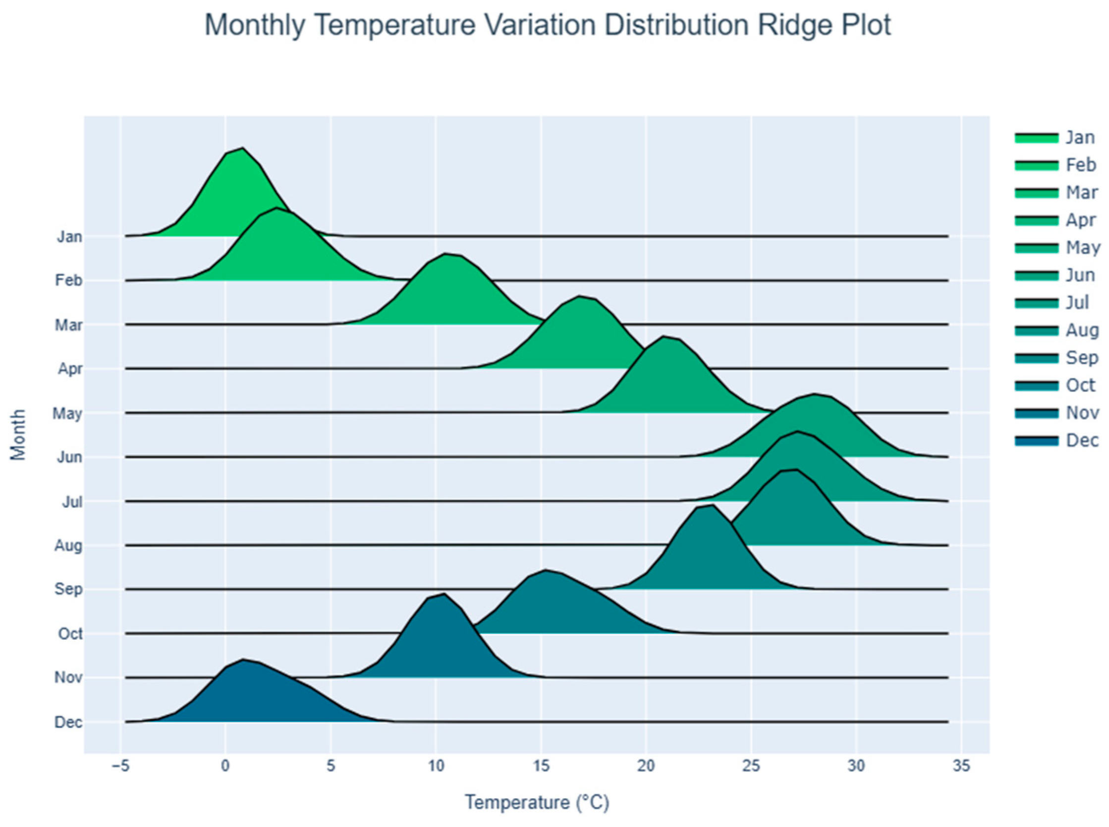
The Baiquan Spring Group in Xinxiang City is currently managed and monitored by the Baiquan Irrigation District Service Center in Huixian County, Henan Province. The existing monitoring data are from January 1964 to May 1979, and the data scale is monthly. From 1979 to 2020, there was intermittent dry-up, and only a brief resumption of flow occurred during the flood season. After the spring area suffered heavy rains in July 2021, it began to resume flow on 24 July, and the data scale is daily. Since the early data before 1979 were on a monthly scale and had a small amount of data, they were not suitable for deep learning modeling, and due to the long-term interruption from 1979 to 2020, they were not of research value. Therefore, this study used the monitoring data from 24 July 2021 to 25 August 2024 as the research object, with a total of 1125 data points. The precipitation and temperature data were sourced from the China National Meteorological Science Data Center. The ridge plot of temperature variation distribution (Figure 2) presents the monthly temperature patterns in the study area, which is of great significance for the research on predicting spring flow based on temperature and precipitation. From January to March, the temperature distribution is concentrated at relatively low values. Under the cold climate, the low temperature will result in weak water evaporation and slow infiltration, thus affecting the recharge of springs. From April to July, the temperature peaks gradually rise. The warming promotes the melting of snow and ice (if any) and enhances the activity of soil moisture, altering the process of precipitation transforming into spring water. From August to October, the relatively high temperature is maintained, accelerating surface evapotranspiration, affecting the groundwater cycle, and being correlated with spring flow. From November to December, the temperature drops. The cooling environment changes processes such as water infiltration. By cooperating with precipitation, it jointly acts on spring flow. Its seasonal cycle provides a crucial dynamic basis of temperature for flow prediction.

2.3. Experimental Setup

The experiments were conducted on a computer equipped with an Intel (TM) I9-13900 processor, an NVIDIA RTX4080 graphics card, 32 GB of RAM, and 16 GB of GPU memory. The model was constructed using the PyTorch (version 11.3) deep learning framework with Python (version 3.9).

3. Methods

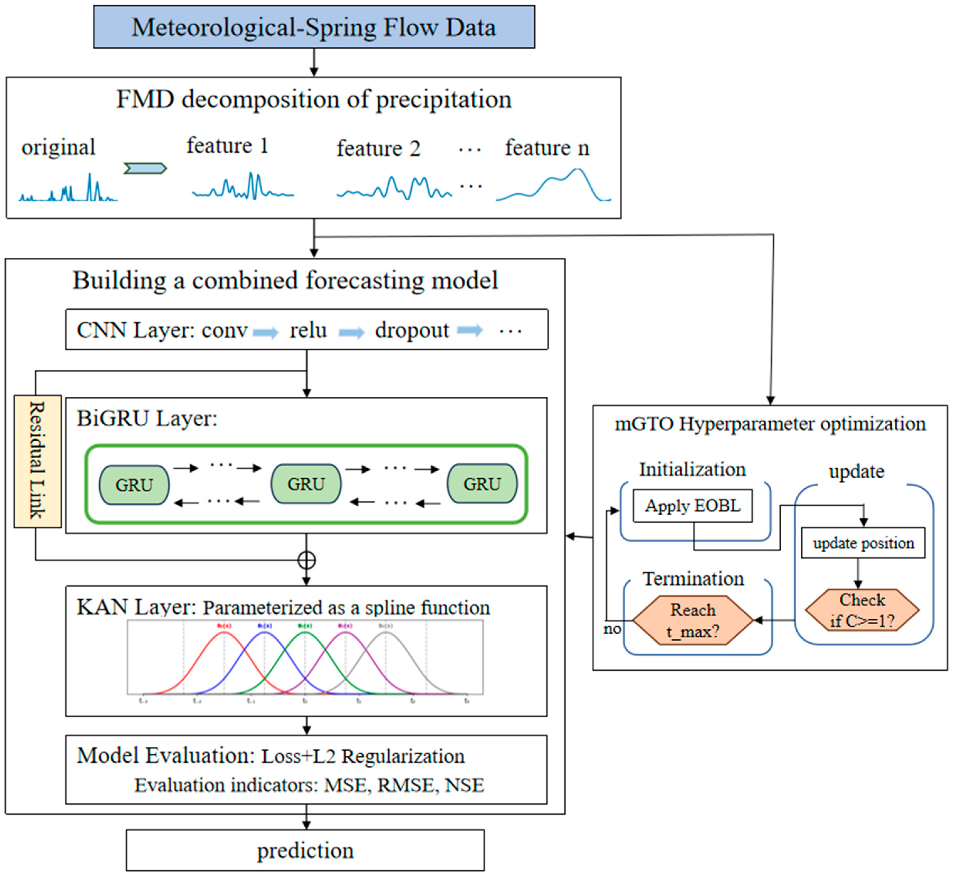
In this study, a new fusion model, FMD-mGTO-BiGRU-KAN, is constructed to dynamically model and predict the water flow of Baiquan Spring. Figure 3 describes the flow chart of this new architecture. FMD performs feature decomposition on the input data, mGTO performs global optimization on the hyperparameters of the prediction model, and constructs a CNN-BiGRU-KAN fusion model for modeling and prediction. Use FMD to perform characteristic mode decomposition on precipitation data, fully extract the impact and periodicity of precipitation, reduce the nonlinear and non-stationarity of the data, capture multi-time scale characteristics, and enable the model to use the influence of precipitation more accurately. The decomposed feature components and temperature data serve as input features for the prediction model, and are subsequently input into the CNN architecture. Through the convolution, activation, and pooling processes, it can automatically learn meaningful local patterns from the data and reduce sensitivity to noise. The features generated by the CNN model are further input into the BiGRU model. The model processes the sequence in both directions, thereby capturing contextual information from both past and future elements, which significantly enhances its ability to grasp the global context of the sequence. The model output layer employs KAN in lieu of the conventional fully connected layer, thereby enhancing predictive performance and improving the model’s interpretability. It is noteworthy that the study implements various strategies to optimize the model’s predictive performance, alleviate overfitting concerns, and strengthen its robustness and applicability. (1) The mGTO intelligent optimization algorithm is introduced to perform global optimization of multiple hyperparameters of the model, making full use of the influence relationship between various parameters to easily achieve good prediction results. At the same time, the use of intelligent optimization algorithms can quickly adapt to different data models in the future, improving the transferability and generalization ability of the model. (2) Adding a residual block structure allows information to be directly transmitted from the CNN layer to the KAN layer, avoiding the “degeneration problem” caused by too many network layers and the gradient attenuation problem caused by multiple nonlinear transformations [36], which helps to maintain the stability of the gradient and speed up the convergence of the network. (3) Add Dropout rate and L2 norm. Due to the interruption of spring flow and the problem of real-world detection, the amount of available data is not very sufficient, so an overly complex network structure is prone to serious overfitting and low generalization ability. Hence, the study employs two regularization strategies, Dropout rate and L2 regularization, to simplify the model, reduce overfitting, and augment the network’s robustness and generalizability. Finally, this study uses MSE, RMSE, and NSE as evaluation indicators and compares with the benchmark models LSTM [37], GRU [31], and Transformer [38]. Through the above multiple designs, this study fully utilizes the effective information of input features, such as precipitation, to establish a prediction model with high accuracy, robustness, and portability, while also reducing the huge training cost of manually adjusting parameters.

3.1. Feature Mode Decomposition

Feature mode decomposition is a novel signal processing technique introduced by Miao et al. [33], which was initially applied to decompose fault signals in rotating machinery. The algorithm employs a non-recursive decomposition approach, utilizing adaptive finite impulse response (FIR) filter banks with varying initializations and updating filter coefficients to select different models (Figure 4). By taking into account the signal’s impulse and periodicity, it demonstrates promising application potential in precipitation feature extraction. The main ideas are as follows:
(1)
Adaptive FIR Filter Bank
In the task of signal decomposition, the filter is a very critical tool. It can “filter” a specific signal by selectively enhancing or suppressing a specific frequency or time-frequency, thus helping to complete the decomposition task. Filters can be divided into two types: analog filters and digital filters according to the type of signal they process. Analog filters use electronic components to simulate circuits and process continuous time signals; digital filters use algorithms such as convolution to process discrete digital signals. FIR is a digital filter implemented in the time domain through convolution. The output depends only on the current and past input values and does not contain feedback loops. The mathematical expression [39,40]:
y [ n ] = j = 0 N 1 k [ j ] x [ n j ]
In the expression, y [ n ] denotes the filter output at discrete time n ; x n j represents the input sample at lag j (with j = 0 corresponding to the current sample), thereby incorporating historical information; h j are the filter coefficients, serving as weighting factors that control the influence of inputs at different lags on the output and are initialized using the window method to satisfy low-pass design requirements; N is the filter order, which determines the length of the input history included in the computation, with higher orders enabling a more detailed characterization of temporal features.
FMD designs an adaptive coefficient adjustment method to improve the traditional FIR filter: The initialization of the filter is performed using a Hanning window-based approach with a defined cutoff frequency, followed by an iterative optimization process to refine the filter coefficients, thereby achieving a filtered signal that closely approximates the target function. The frequency band of the original signal is partitioned into K equal sub-bands during the initialization phase, and the upper and lower cutoff frequencies, denoted as f t and f e , respectively, are determined for each sub-band as follows:
f t = k f j / 2 K f e = ( k + 1 ) f j / 2 K k = 0 , 1 , 2 , K 1
where f j denotes the original signal’s sampling frequency. A new filter bank is created using Formula (2), consisting of filters with different cutoff frequencies that are uniformly distributed across the original frequency spectrum.
(2)
Filter Update and Period Estimation
FMD selects correlated kurtosis (CK) as its objective function. A high CK value corresponds to the presence of significant spiky impulses within the signal (e.g., short-duration intense precipitation), while a low CK value indicates a flatter signal distribution (e.g., sustained weak precipitation or noise). The FMD framework is transformed into a constrained optimization problem, with the constraint equation formulated as follows:
argmax { f k ( j ) } C K M u k = n = 1 N m = 0 M u k n m T s 2 / n = 1 N u k ( n ) 2 M + 1
By identifying a set of filter coefficients f k ( l ) that maximizes the objective function C K M u k , the mode maximizing kurtosis preferentially focuses on the impulsive characteristics of heavy rainfall. This process effectively separates these features from sustained light rainfall and background noise, thereby providing an enhanced signal foundation for precipitation intensity classification and extreme weather warning systems. The numerator n = 1 N m = 0 M u k n m T s 2 is the sum of the squares of the products of u k ( n ) at different time points n m T s ( m from 0 to M), which reflects the correlation of the signal over multiple delay periods; the denominator normalizes the numerator to enhance the rationality of comparison between different signals.
u k ( n ) = j = 1 J f k ( j ) x ( n j + 1 )
shows that u k ( n ) is the result of filtering the original signal x n through the kth FIR filter f k   of length J . In this convolution operation, x ( n j + 1 ) is the sampling point of the original signal, and the filtered signal u k ( n ) is obtained by summing the products of different j coefficients and corresponding sampling points. The objective function is defined as:
C K M ( u k ) = f k H X H W M X f k f k H X H X f k = f k H R X W X f k f k H R X X f k
In practice, accurately estimating the signal period is challenging. To overcome this problem, the IMCKD technique is adopted to estimate the signal period from the measured signal, leveraging the principles of autocorrelation theory. At the period position, the autocorrelation spectrum exhibits a pronounced local maximum, and the first occurrence of this maximum after the zero point is identified as the estimated period. As the FIR filter is updated, the estimated period is refined, becoming increasingly accurate.
(3)
Mode Selection
The modes representing precipitation characteristics may encompass components such as seasonal periodicities, short-term rainfall impulses, and noise. The presence of redundant modal components leads to the occupation of computational resources by repetitive information, thereby increasing processing overhead. Furthermore, redundant modes may introduce extraneous interference, obscuring critical precipitation features and diminishing the accuracy and interpretability of the decomposition results. The Correlation Coefficient (CC) quantifies the similarity between two modes; a high CC value indicates significant redundant information shared between them. Consequently, the CC is incorporated as a modal selection strategy, wherein the mode exhibiting the maximum CK value is selected, as defined below:
C C b d = n = 1 N u b ( n ) u ¯ b u d ( n ) u ¯ d n = 1 N u b ( n ) u ¯ b 2 n = 1 N u d ( n ) u ¯ d 2
where u ¯ b and u ¯ d are the means of u b and u d respectively. The resulting CC value is bounded between −1 and 1. The proximity to 1 indicates a higher degree of correlation between the two modes, suggesting that they share a larger number of identical components. To eliminate mode aliasing and redundancy caused by multiple modes containing shared components, the two modes with the highest correlation coefficient are identified. The mode with the lower CK value is then discarded, thereby retaining the more informative one.
The FMD decomposition algorithm considers both the impulsive and periodic characteristics of the signal, thereby enhancing its robustness to interference and noise. The adaptive FIR filter facilitates the extraction of decomposition patterns without being constrained by filter parameters such as shape, bandwidth, and center frequency, thereby yielding a more comprehensive decomposition. In this study, FMD is used to decompose precipitation, and the decomposition results are input into the fusion prediction model for prediction.

3.2. Bidirectional Gated Recurrent Unit

The Gated Recurrent Unit (GRU) is a streamlined recurrent neural network architecture designed to address the vanishing and exploding gradient problems in Recurrent Neural Networks (RNNs) when processing long-sequence data. Its core mechanism employs an update gate ( z t ) and reset gate ( r t ) to precisely regulate information flow, thereby effectively capturing long-term dependencies in time series. The update gate ( z t ), computed from the current input and previous hidden state with output values in [0, 1], dynamically balances historical information retention: When z t approaches 1, greater proportions of historical information from prior hidden states are preserved to maintain memory of long-term sequential features; when z t approaches 0, the model prioritizes current inputs to adapt to abrupt changes. The reset gate ( r t ), similarly generating outputs 0 , 1 based on current inputs and previous hidden states, primarily filters and discards irrelevant historical information: When rt approaches 0, it suppresses redundant historical data to reduce interference; when rt approaches 1, it permits retention of valid historical information to sustain temporal continuity. A candidate hidden state is generated by integrating current inputs with the reset-gate-modulated prior hidden state, enabling refined feature extraction. The final hidden state is then produced through linear interpolation by the update gate, adaptively fusing previous hidden states with candidate states. This architecture allows GRUs to preserve critical long-term dependencies while precisely responding to short-term perturbations when processing complex long-sequence hydrological data.
z t = σ ( W z [ h t 1 , x t ] )
r t = σ ( W r [ h t 1 , x t ] )
h ˜ t = tanh ( W [ r t h t 1 , x t ] )
h t = 1 z t h t 1 + z t h ˜ t
where W z , W r and W are weight matrices. The outputs of the update and reset gates are constrained between 0 and 1. The update gate’s output approaching 1 signifies a greater retention of the previous state, while the reset gate’s output approaching 0 indicates a more significant forgetting of historical information.
Bidirectional Gated Recurrent Unit is a bidirectional architecture developed based on GRU. Traditional GRU can only process sequence data in order, calculating hidden states from front to back. BIGRU contains both forward and reverse GRU, and can process input sequences from two directions at the same time (Figure 5), thereby better capturing contextual information in the sequence. The forward GRU processes the input data in chronological order from the beginning to the end of the sequence, and its calculation process is the same as that of the ordinary GRU; the reverse GRU processes the input in chronological order from the end to the beginning of the sequence, and its calculation process is similar to that of the forward GRU, but the input order is reversed. The final output concatenates the hidden states of the forward and reverse GRU at the same time, namely:
h t B = [ h t , h t ]
h t and h t denote the forward and reverse hidden states at time step t , respectively. This approach allows the BiGRU model to comprehensively utilize information from both preceding and succeeding time steps. The forward GRU captures the forward-propagating influence of historical meteorological conditions on the current flow (e.g., direct recharge from yesterday’s rainfall to today’s flow). In contrast, the backward GRU mines the backward-propagating constraints imposed by future meteorological conditions on the current flow (e.g., correction for today’s evaporative loss due to tomorrow’s temperature drop). This synergistic action enables a more thorough characterization of the non-linear lagged relationships among precipitation, temperature, and spring flow. Consequently, it overcomes the incomplete modeling of lag effects inherent in unidirectional models that rely solely on historical data, thereby enhancing prediction accuracy. Compared to traditional RNN and LSTM models, BiGRU’s bidirectional fusion mechanism fully resolves multi-scale temporal dependencies, preventing information loss. Furthermore, its more streamlined architecture and fewer parameters relative to LSTM lead to higher training efficiency and superior generalization ability, especially in hydrological scenarios characterized by small sample sizes and high noise levels. This allows the model to strike an effective balance between accuracy and computational efficiency.

3.3. Kolmogorov–Arnold Networks

The Kolmogorov–Arnold Networks [32] embodies a pioneering theoretical neural network paradigm rooted in the Kolmogorov—Arnold representation theorem. This model departs from traditional Multilayer Perceptrons (MLPs) by employing learnable spline functions in place of fixed activation functions, substituting each weight with a parameterized univariate function. This provides exceptional flexibility, as splines dynamically learn via coefficient optimization rather than adhering to a static form. Their piecewise construction ensures superior local adaptability to input variations, overcoming the limitations of global activation functions in capturing local features. This local sensitivity and flexibility lead to high parameter efficiency, allowing the model to approximate complex functions with a minimal set of parameters, thereby improving generalization and reducing the risk of overfitting in high-dimensional contexts. It fundamentally eliminates the dependence on linear weight matrices and reduces the problems caused by the high dimensions of traditional models. The core calculation graph formula is as follows:
f ( x ) = d = 1 2 n + 1 Φ d b = 1 n ϕ d , b ( x b )
Functions Φ d and ϕ d , b are expressed as B-spline curves, and the target function is approximated by learning the spline curve parameters. The B-spline function is generally expressed as:
s p l i n e ( x ) = i c i B i ( x )
The coefficients c i is optimized during training to achieve the best fit, and B i ( x ) corresponds to the B-spline basis functions that are defined over a grid structure. The distribution of grid points determines the effective domain of each basis function. Adjusting the sparsity and density of grid points systematically controls the functional characteristics: sparse configurations extend the influence of basic functions to achieve greater smoothness through averaging effects, while dense arrangements restrict effective intervals to permit localized rapid variations in the function, thereby reducing overall smoothness but enhancing the ability to capture fine details. Furthermore, the grid distribution regulates the smoothness of the entire function space by modulating the overlap regions between adjacent basis functions, where increased overlap produces smoother transitions between segments. Adaptive grid adjustment through dynamic updating enables the system to automatically respond to input data distributions by locally refining grids in regions of high functional variability while maintaining coarse grids in relatively stable domains. This strategy ensures modeling flexibility while preventing parameter redundancy. Grid extension techniques, which minimize the distance between coarse-grid and fine-grid basis function representations, consequently play a critical role in determining both the global morphology and local smoothness properties of the resultant spline curves. The network is stacked and deepened by the KAN layer matrix Φ = { ϕ q , p } composed of 1D functions. The KAN network with a depth of L is expressed as:
K A N ( x ) = ( Φ L 1 Φ L 2 Φ 1 Φ 0 ) x s
The activation function is specifically initialized using the residual activation function ϕ ( x ) = w b b ( x ) + w s s p l i n e ( x ) , and the spline grid is dynamically updated based on the input activation. Unlike conventional MLP models that rely on linear weight matrices for feature transformation, the KAN framework employs univariate spline functions to replace traditional linear weights. The localized nature of spline basis functions allows for decoupled feature transformations, where individual function behaviors can be examined in isolation without interference from other model parameters, thereby achieving superior transparency in functional mapping mechanisms. To enhance the interpretability of the model, the Kolmogorov—Arnold Network (KAN) adopts simplification techniques. Specifically, it defines the L1 norm of the activation function as | ϕ | 1 1 N p s = 1 N p ϕ x ( s ) and the L1 norm of the KAN layer as | Φ | 1 i = 1 n i n j = 1 n o u t | ϕ i , j | 1 [41], while introducing an entropy regularization term denoted as S ( Φ ) i = 1 n i n j = 1 n o u t | ϕ i , j | 1 | Φ | 1 l o g | ϕ i , j | 1 | Φ | 1 . The overall training objective is formulated as l t o t a l = l p r e d + λ μ 1 j = 0 J 1 |   Φ j | 1 + μ 2 j = 0 J 1 S Φ j . This architectural design facilitates network sparsity by enabling the model to retain only essential functional components, resulting in a well-defined structural organization. The implementation of spline functions serves dual advantages: they permit shape visualization and can be converted into known symbolic functions, thereby achieving a transition from numerical fitting to symbolic formulations. This transformation allows model behavior to be expressed through human-interpretable mathematical representations. Finally, KAN initializes the fine grid parameters based on the existing coarse grid by minimizing the distance between the new fine grid function and the coarse grid function. Solving the optimization function c j = a r g m i n c j E x ~ p ( x ) j = 0 G 2 + k 1 c j B j ( x ) i = 0 G 1 + k 1 c i B i ( x ) 2 to determine the fine grid parameters c j . This study uses the KAN layer to replace the fully connected layer of the traditional model as a parameter of the prediction output layer to construct the fusion model.

3.4. An Improved Gorilla Troops Optimizer

Inspired by the collective behavior of gorillas, the Gorilla Troops Optimizer (GTO) is a metaheuristic algorithm designed to solve optimization problems. GTO simulates the social structure and behavior of gorilla troops to perform optimization operations. The algorithm comprises two primary stages: exploration and development, with distinct mechanisms applied during each stage to facilitate effective optimization.
During the exploration phase, three distinct mechanisms were devised, with their corresponding calculation formulas being:
G X t + 1 = U B J B × e 1 + J B , r a n d < p , e 2 C × X e ( t ) + J × D , r a n d 0.5 , X ( t ) J × J × X t G X e ( t ) + e 3 × X t G X e ( t ) , r a n d < 0.5 .
where represents the gorilla’s present position vector, and G X ( t + 1 ) denotes the prospective position in the following iteration. When r a n d < p , where p is a parameter between 0 and 1 that dictates the probability of mechanism selection, and e 1 is a random value between 0 and 1, the algorithm proceeds to the unknown position mechanism, with U B and J B representing the variable’s upper and lower limits. This mechanism facilitates the algorithm’s ability to perform comprehensive explorations within the problem space, thereby enhancing the discovery of novel potential solution regions. When r a n d 0.5 , the mechanism of moving to other gorillas is calculated by the formula:
C = F × 1 I t M a x I t
F = c o s ( 2 × e 4 ) + 1
J = C × j
D = Z × X ( t )
I t denotes the current iteration number, M a x I t is the total iteration count, e 2 ~ e 4 represents random values between 0 and 1, j is a random number in the interval [−1, 1], and Z is a random quantity within the bounds of C , C . This mechanism promotes a balance between exploratory and developmental aspects. When the algorithm is in condition r a n d < 0.5 , it serves as a mechanism for relocating to a known position. As a result, this mechanism significantly enhances the algorithm’s ability to search various optimization spaces and assists in avoiding local optima.
During the update phase, use the “Follow the Silverback” mechanism and the competition for adult females mechanism to conduct more refined searches and improve search performance.
“Follow the Silverback” mechanism: The entire troop of gorillas abides by the Silverback gorilla’s decisions. The mechanism is triggered at C W :
GX ( t + 1 ) = J × H × ( X ( t ) X s ) + X ( t )
Competition for adult females: This means that young gorillas challenge the original leader and compete for female gorillas. When C < W , the mechanism is triggered:
GX ( t + 1 ) = X s ( X s × Q X ( t ) × Q ) × A
where X s denotes the optimal position vector. Upon completion of the update phase, the fitness values of all G X individuals are evaluated. If a fitness value meets condition   G X t < X t , the corresponding individual G X t is adopted as the new individual, and the optimal solution discovered during the search is designated as the new silverback gorilla.
mGTO is an enhanced version of GTO, addressing its propensity to converge prematurely and get trapped in local optima when tackling complex optimization tasks. It integrates Elite Opposition-Based Learning (EOBL) [42] into the initialization and update phases to enhance the initial solution quality and population diversity. Furthermore, mGTO combines GTO with the Cauchy Inverse Cumulative Distribution (CICD) and Tangent Flight Operator (TFO) to bolster its local search capabilities, balance the search strategy, and improve convergence, thereby avoiding local optima. The main improvements are as follows:
Initialization phase: Use EOBL technology to generate the initial population. For the given problem, the reverse position x ^ k , j = ( x ^ k , 1 x ^ k , 2 x ^ k , D ) of the individual X k = ( x k 1 , x k 2 , x k D ) in the population is calculated by x ^ k , j = F × ( d y j + d z j ) x k , j , where F 0 , 1 is the generalization factor and the dynamic boundary d y j = min ( x k , j ) to d y j = max ( x k , j ) . If x ^ k , j < y j or x ^ k , j > y j , then x ^ k , j = r a n d ( y j + z j ) . This approach leverages elite individuals to direct the population toward the optimal solution, simultaneously promoting population diversity.
Update phase: Improved “Follow the Silverback” mechanism: Based on the original “Follow the Silverback” mechanism of GTO, CICD operator is added. The improved model:
X ( t + 1 ) = X ( t ) + J × H × ( X ( t ) X s ) × ( 0.01 t a n ( π ( p 1 2 ) ) )
The calculation method of J and H is the same as the original algorithm, p = r a n d a n ( 1 , d ) . This enhancement decreases the gap between the gorilla and the silverback gorilla, resulting in a rapid reduction in the final step size, thereby facilitating a quicker convergence to the optimal target value. Improve the “competition for adult females” mechanism: Add the TFO operator to the “competition for adult females” mechanism, and the improved formula:
X ( i ) = X s ( X s × P X ( t ) × P ) × t a n ( v π 2 )
Among them, P = 2 × r 5 1 and v are random numbers uniformly distributed in the range of 0 ,   1 , and r 5 ranges from 0 to 1. The TFO operator can balance exploration and development search and control the step size to avoid insufficient precision.
This study applies the mGTO algorithm to optimize critical hyperparameters in the hybrid model architecture, with training loss specifically designated as the fitness function. This strategic implementation enables accelerated convergence during model training while simultaneously enhancing precision in parameter estimation.

3.5. Evaluation Indicators

To comprehensively evaluate the performance of the proposed model and the benchmark models, this study employs Mean Squared Error (MSE), Root Mean Squared Error (RMSE), and Nash-Sutcliffe Efficiency (NSE) as evaluation metrics. The specific formulas are as follows:
M S E = 1 n i = 1 n ( y i y ^ i ) 2
R M S E = 1 n i = 1 n ( y i y ^ i ) 2
N S E = 1 ( Q o , i Q s , i ) 2 ( Q o , i Q o ) 2

4. Results

4.1. Determination of Parameters of FMD Characteristic Modes

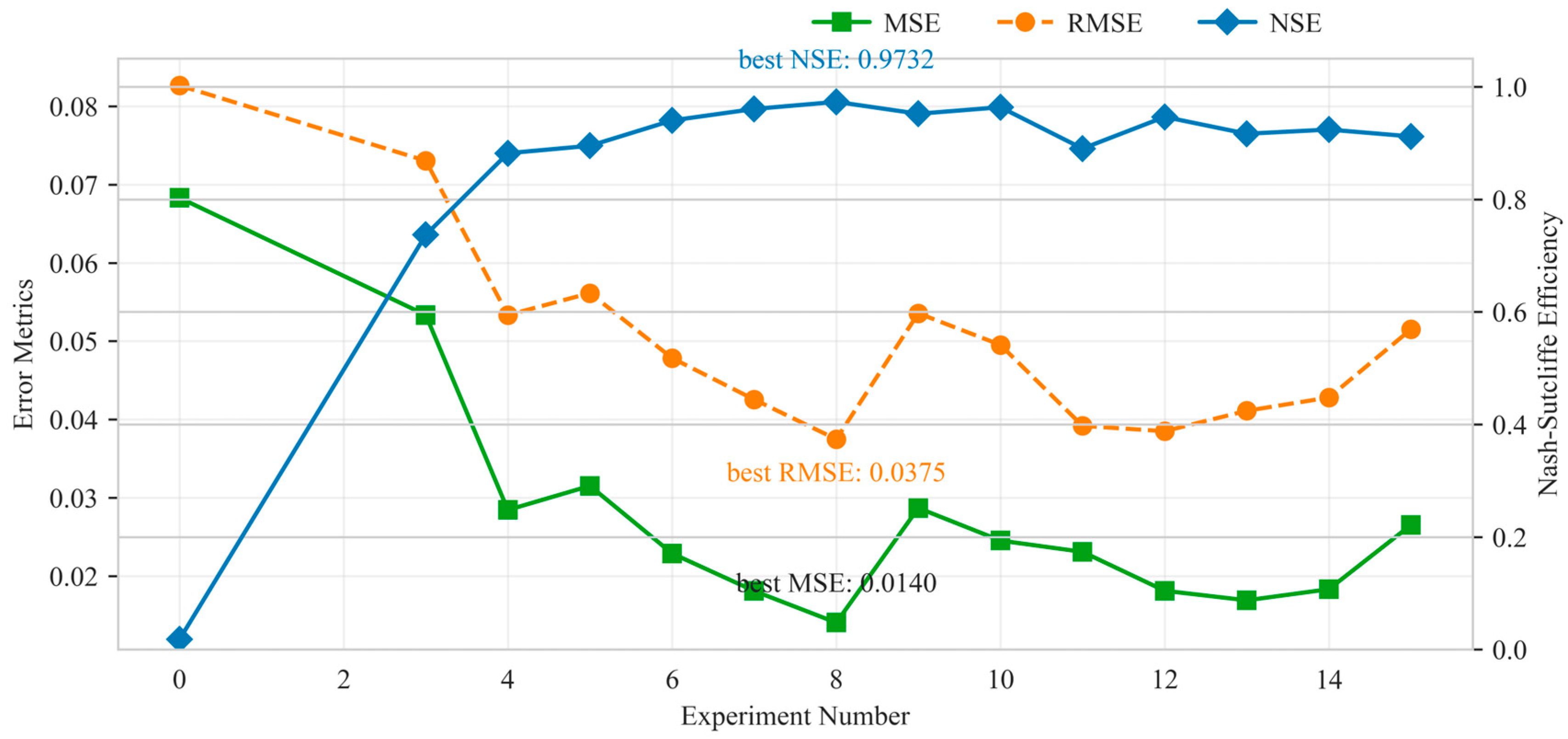
This study used precipitation and average temperature to predict spring flow. As shown in Figure 6, the original data without decomposition was used to directly model the model. The MSE and NSE of the prediction were 0.06831 and 0.0179, respectively, which is a very poor result. After decomposition, the prediction accuracy began to improve significantly, indicating that the use of FMD has a huge improvement in the modeling and prediction of spring water flow. In the FMD decomposition process, the number of modes needs to be determined according to the actual data. In order to find the optimal decomposition characteristic number, this study decomposes the precipitation data starting from n = 3 and gradually increasing by 1. The maximum decomposition number is 15. The decomposition results are input into the model for modeling. Through 16 rounds of operation, the average results of multiple runs in each round are taken to calculate various evaluation indicators.
As shown in Figure 6, when the number of modes is 8, the MSE and RMSE are the smallest, which are 0.014 and 0.0375, respectively, and the NSE is the largest at 0.9732, which has very good prediction accuracy. For decomposition numbers less than 8, an increase in the number of decompositions results in a gradual reduction in loss and a corresponding improvement in NSE; in contrast, when the number of decompositions surpasses 8, the NSE tends to decrease and the loss tends to increase, despite some fluctuations in the indicators. Therefore, choosing 8 as the number of decompositions is reasonable and effective.
As illustrated in Figure 7, the Baiquan area is situated in the northern region of the North China Plain, characterized by highly uneven precipitation, which results in significant nonlinearity and instability in the original precipitation data. Direct use not only fails to provide effective information for the model but also causes interference. FMD is used to decompose this nonlinearity and transform high-frequency oscillation features into smooth features that can be better recognized and utilized by the model. When there are too few decomposed modes, the features cannot be extracted completely and effectively, and the decomposition results are still unstable to a certain extent; when there are too many decomposed modes, redundant information and unnecessary noise are easily introduced, resulting in greater error in the results, which is not conducive to the next step of analysis. Therefore, the appropriate number of features has an important impact on research and analysis.

4.2. Intelligent Optimization Algorithm for Hyperparameter Optimization

This study uses a mature and efficient intelligent optimization algorithm to optimize the model’s hyperparameters to obtain more accurate and robust model parameters. In deep learning experiments, the time window length (look back), learning rate, number of training rounds (num epochs), and batch size have an important influence. The choice of look-back period influences the number of past observations that are used to forecast future values in a time series model, which affects its ability to identify temporal dependencies; learning rate controls the parameter update step size, affecting the model’s convergence speed and stability; num epochs determines the number of times the model traverses the training set, affecting training adequacy and overfitting risk; batch size represents the count of samples processed together for a single parameter update, influencing the trade-off between memory usage and the precision of gradient estimation. At the same time, these hyperparameters have a significant mutual influence relationship, and their synergistic effect will jointly affect the model performance and training efficiency. Therefore, hyperparameter selection is an important factor affecting the model. In this study, the mGTO algorithm is employed to optimize the aforementioned four hyperparameters. The parameters of mGTO are configured as follows: 100 iterations, a population size of 50, and a probability of 0.03. The range for hyperparameter tuning is presented in Table 1:
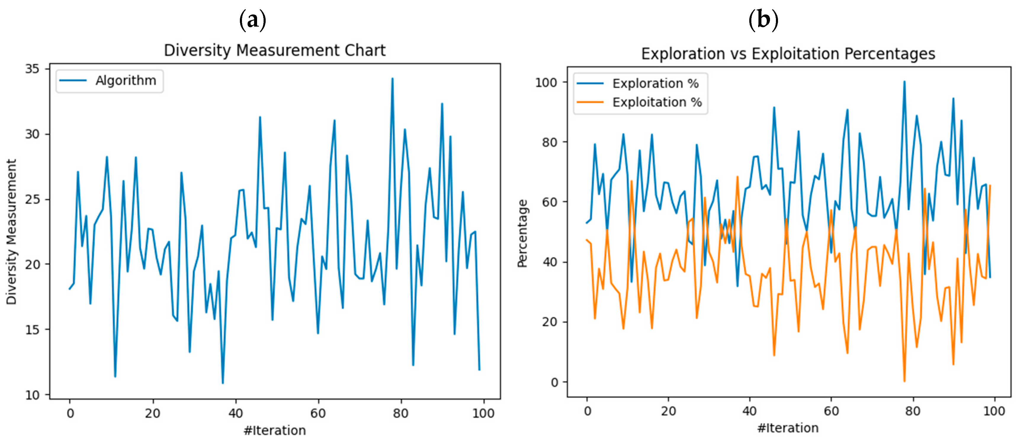
Figure 8a shows the changes in the population during the optimization process. At some iteration points, the population diversity dropped sharply. For example, when it was close to the 40th iteration, the diversity value dropped from about 20 to close to 10, indicating that the algorithm focused on exploring certain local areas at these stages, resulting in a decrease in the differences between individuals in the population and a decrease in population diversity. At other iteration stages, the diversity value rose rapidly. For instance, during the 60th to 80th iterations, the value repeatedly surged from a relatively low level to over 30, demonstrating the algorithm’s capability to re-explore various regions of the solution space. This re-exploration enhanced the population’s diversity, thereby facilitating the escape from local optima and the continued pursuit of improved solutions. The population size is generally maintained between 15 and 30, and a certain diversity can be maintained in most iterations, with the ability to continuously explore new solution space areas. Figure 8b depicts the exploration and exploitation percentages as blue and orange curves, respectively. The observation that the exploration percentage is generally higher than the exploitation percentage implies that the algorithm is biased towards exploring new regions of the solution space, which enables it to identify potentially better solutions and avoid getting trapped in local optima prematurely. Near the 40th and 80th iterations, the development ratio increases significantly, indicating that the algorithm focuses on deep mining and optimization of the discovered better solution areas.
The global fitness shows an overall decline during the optimization process (Figure 8c). In the early stage of the iteration, the fitness drops rapidly, and drops to about 0.3 around the 20th iteration. After that, it shows a trend of staged decline. After each decline, it will remain stable within a certain range until the next decline, indicating that the optimization algorithm can quickly find a better solution at the beginning, causing the target value to drop significantly. With the progression of the iterations, the algorithm can continue to improve the solution and eventually converge, always effectively optimizing in the direction of the optimal solution. Finally, when it is close to the 100th iteration, the fitness drops to about 0.15, and finally, a good result is obtained, indicating that the optimization result can be used for modeling. The running time of each round of iteration is not fixed (Figure 8d). Although the running time also fluctuates, it generally fluctuates between 1000 and 1400 s, especially after 80 rounds. It generally shows a downward trend, indicating that the computational efficiency of the algorithm is improving. The above results show that the global optimization of mGTO obtains a reasonable and effective result, so the optimization result is used as the model training parameter. The results are shown in Table 2:

4.3. Comparison of Prediction Effects of Different Models

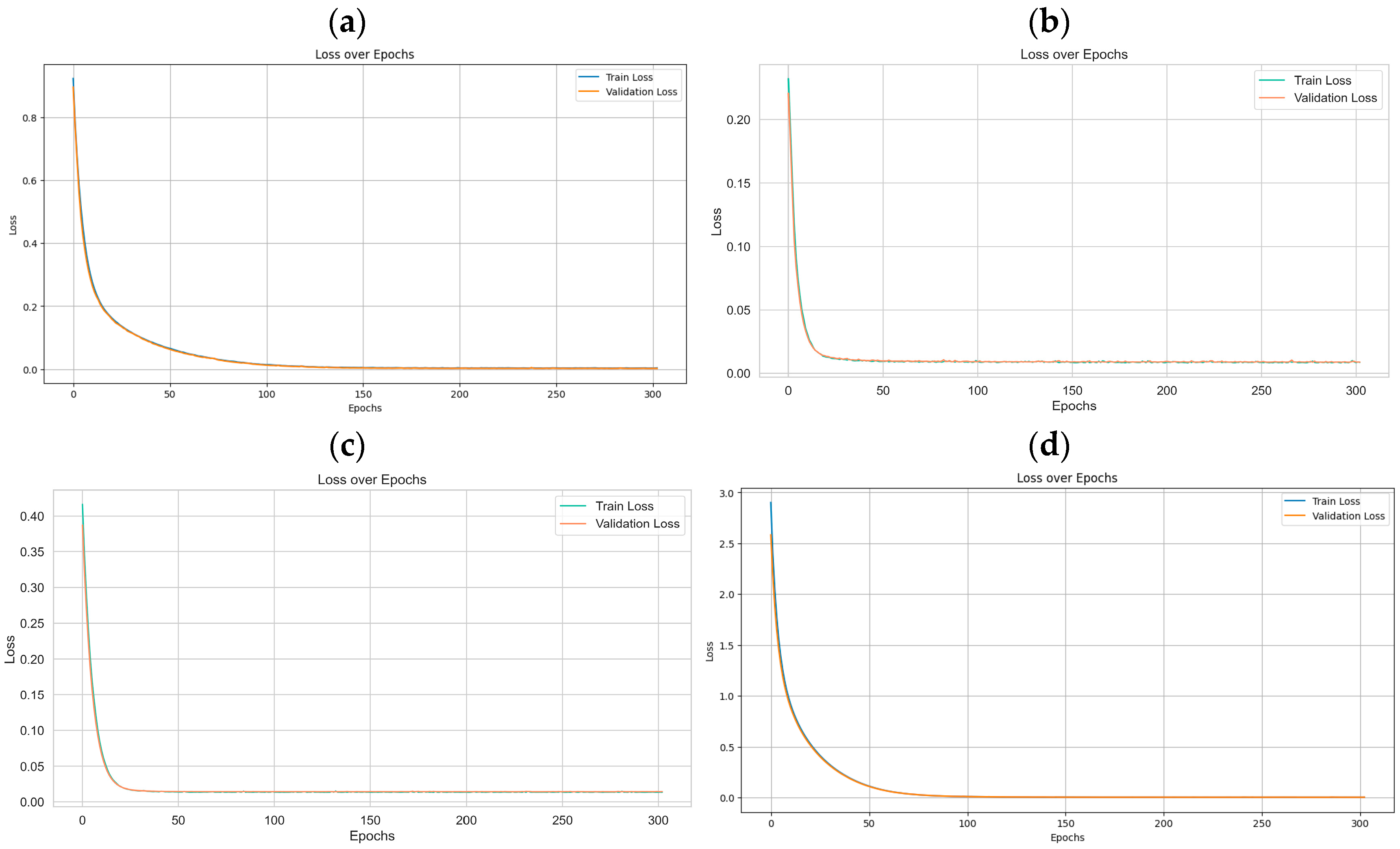
In this study, the FMD-mGTO-BiGRU-KAN architecture was constructed as a prediction model to predict the water flow of Baiquan Spring. We split the data into three distinct sets: training, validation, and Prediction set, in the ratio of 70:15:15. To compare the performance of this model, we used the currently popular spring flow prediction models, LSTM, GRU, and Transformer as benchmark models for comparative analysis. Since all benchmark models had very poor prediction results using the original data, with an accuracy of less than 0.1, they lost their significance as benchmark models for comparison. Therefore, all four groups of models used FMD-decomposed data for modeling. To ensure the reliability of the comparison results, the same data partitioning method and architecture parameters were used, and the average value was taken through multiple repeated experiments for analysis. Figure 9 shows the change of MSE with the number of iterations during the training and verification process of FMD-mGTO-BiGRU-KAN and three comparison models. It can be seen that the loss of the four models decreases smoothly during the training process and eventually stabilizes, indicating that there is no overfitting phenomenon. At the same time, it can be seen that the descent process of Figure 9a,d is smoother, indicating that the training process is more robust.
Table 3 shows the MSE, RMSE, and NSE values of the constructed FMD-mGTO-BiGRU-KAN and three benchmark models in the training, validation, and prediction processes. The model accuracy is greater than 0.87, and all have good prediction performance. By comparison (Figure 10), it is found that the FMD-mGTO-BiGRU-KAN model performs best in all results among the four groups of models. The MSR and RMSE in the training set are reduced by 61.11% and 37.19% respectively, compared with the average values of the comparison models, and the prediction process is reduced by 82.47% and 50.15% respectively. The NSE in training, validation, and prediction is increased by 6.98%, 7.10%, and 8.01% respectively, and the prediction accuracy is as high as 0.9825. The model has an accurate prediction ability and is more robust. The losses of the four models all increase in prediction, but the increase of FMD-mGTO-BiGRU-KAN is much smaller than that of the comparison model, indicating that this model has excellent generalization ability and robustness. GRU performed the worst, mainly because its architecture is relatively simple, sacrificing some prediction accuracy. LSTM and Transformer performed similarly, with Transformer performing slightly better in training and validation sets, but slightly worse in the prediction process, indicating that Transformer has a slight overfitting phenomenon due to its overly complex structure.
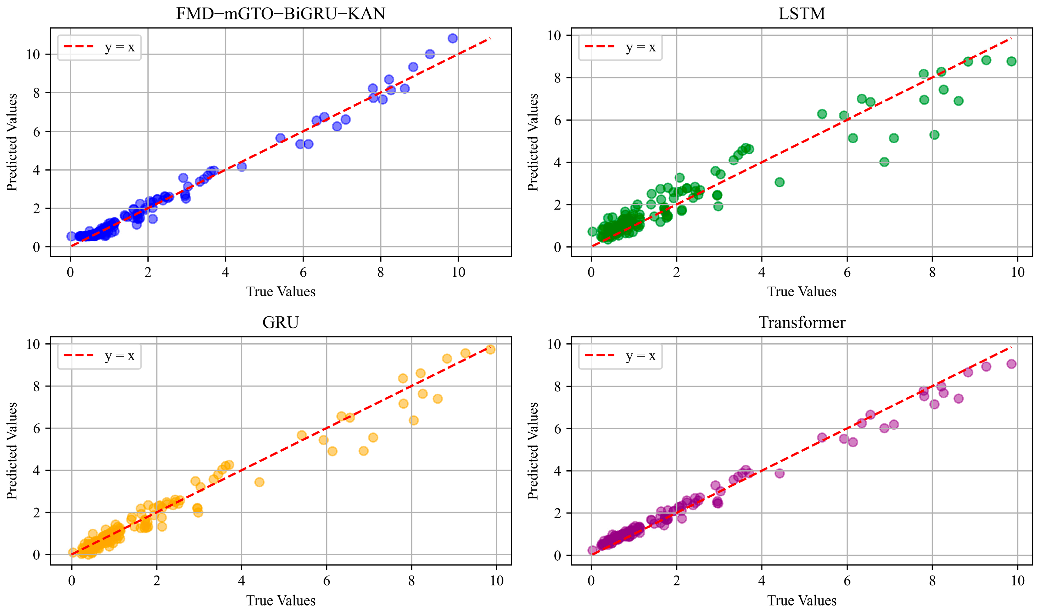
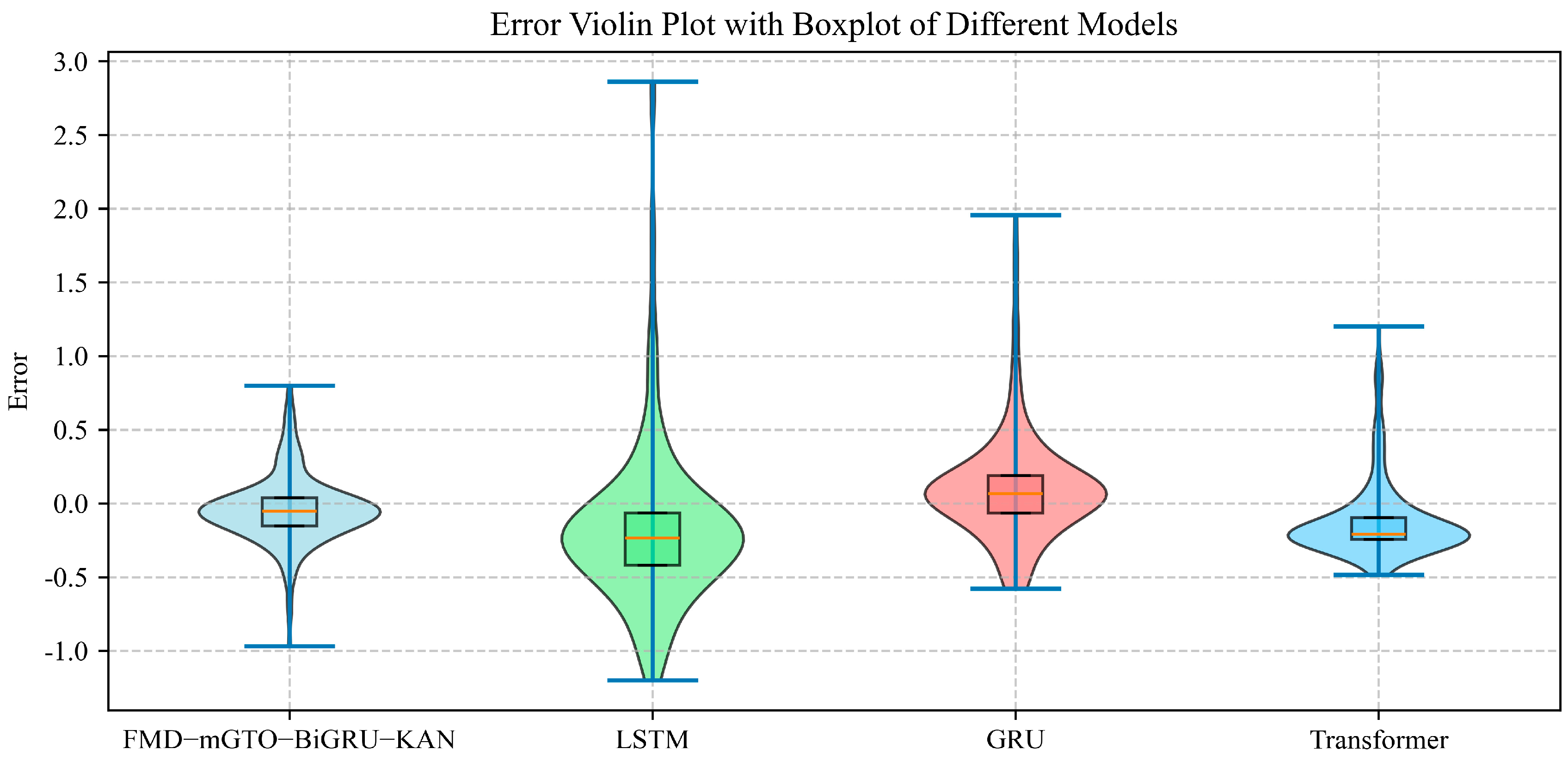
Figure 11 and Figure 12 show the prediction errors of the four models. The red dotted line of y = x in Figure 11 red dotted line, representing y = x , demonstrates the correlation between predicted and true values. The scatter points’ closeness to the line is indicative of the model’s prediction accuracy. It is evident from the figure that the FMD-mGTO-BiGRU-KAN model achieves the highest concentration of points, with a uniform distribution of errors across stages near the dotted line. The distribution of LSTM and GRU is relatively discrete, especially when the true value is large; Transformer predicts larger values when the true value is small, and smaller values when the true value is large, and the prediction ability of the peak value is insufficient. Figure 12 shows the distribution of prediction errors. The violin plot of the FMD-mGTO-BiGRU-KAN model is narrow, indicating that the error value distribution is relatively concentrated, the median (horizontal line in the box) is close to 0, and the box is short, indicating that most of the errors are concentrated in a small range, the degree of dispersion is low, and the model prediction error is small and stable. The violins of LSTM and GRU are wide and have extreme values, indicating that the prediction is unstable. The median of Transformer is close to −0.25, and the overall error is large and uneven.

5. Conclusions

Detecting and forecasting spring flows is a task that is critical to the sustainable development and utilization of springs, but the complex structure of the groundwater system makes it difficult to predict using conventional methods. This study proposes a relocatable hybrid deep learning architecture of FMD-mGTO-BiGRU-KAN for Baiquan water flow prediction. This architecture integrates different algorithms and uses targeted algorithms for different stages of prediction: FMD is used in the data stage to perform feature decomposition of precipitation, which can cope with feature data of different noises. mGTO is used in the parameter selection stage to perform global optimization of hyperparameters, and the most suitable hyperparameter combination can be quickly found for any data and model, thereby improving the model’s transferability and generalization capability. BiGRU-KAN is used in the prediction stage. The BiGRU architecture is adopted to handle time series data, identify data in both directions at the same time, and improve the ability to identify and simulate historical laws. KAN eliminates the traditional reliance on linear weight matrices, reduces the problems caused by the high dimensionality of traditional models, and improves the interpretability of the model. The primary conclusions drawn from this research are presented below:
(1) FMD was used to decompose precipitation data. Through multiple experiments, the effects of different decomposition numbers on model performance were explored (Figure 6). The results show that when decomposition is not used, due to the serious nonlinear and irregularity of precipitation, the model prediction effect is extremely poor, and the prediction accuracy is close to 0 (the performance is consistent in the benchmark model). Starting from the number of decompositions of 3, the model performance began to improve significantly. When the number of decompositions is 8, the MSE and RMSE reach the minimum, which are 0.014 and 0.0375, respectively, and the NSE reaches the maximum of 0.9732. When the number of decompositions continues to increase, the volatility of MSE and RMSE begins to increase, and the volatility of NSE decreases. Our findings suggest that decomposing the data into 8 features yields the best model performance. When the number of decompositions is insufficient, effective information cannot be fully mined. When the number of decompositions is too large, new noise is easily introduced, resulting in information redundancy. Compared with the use of original data, the introduction of FMD effectively utilizes the feature data that was originally unusable, consequently leading to a significant enhancement in the model’s predictive performance. Meanwhile, the application of FMD in the benchmark model also greatly improves the prediction effect, indicating that FMD has significant transferability.
(2) Use mGTO to globally optimize the model hyperparameters to avoid local optimal problems caused by manual debugging. mGTO is a further optimization and improvement based on the excellent intelligent optimization algorithm GTO, and has excellent performance. By introducing the intelligent optimization algorithm, on the one hand, we can better utilize the mutual influence factors between hyperparameters to avoid falling into local optimality, optimize the model’s overall effectiveness, and reduce the time and equipment costs caused by manual adjustment of parameters. On the other hand, the intelligent optimization algorithm is transferable. In the future, when modeling spring flow data in different regions or adjusting the model architecture, we can search for the best hyperparameter combination globally more quickly, reduce training costs, and improve model performance.
(3) Compared with other commonly used models (Figure 10), the FMD-mGTO-BiGRU-KAN hybrid deep learning architecture has a more accurate and robust prediction effect. During the training, validation, and testing process, it has lower prediction loss and higher prediction accuracy. The MSE and RMSE in the test set are 82.47% and 50.15% lower than the comparison model on average, and the prediction NSE is as high as 0.98, which is 8.01% higher than the baseline model on average. The model’s predictive performance is outstanding. As evidenced by the analysis of prediction errors (Figure 11 and Figure 12), the proposed model exhibits a smaller, more concentrated, and uniformly distributed prediction error, thereby demonstrating its superior predictive stability and robustness.

6. Discussion

The prediction model developed in this study demonstrates substantially enhanced accuracy compared to existing research, where FMD decomposition significantly improved model performance (original data Nash-Sutcliffe Efficiency/NSE = 0.0179). This aligns with findings by Zhou et al. [14,18], confirming the efficacy of time-frequency decomposition for nonlinear hydrological data. By optimizing the modal number ( n = 8 ), our approach better accommodates daily-scale precipitation data characteristics and overcomes limitations of conventional decomposition methods in extremely small-sample scenarios. The BiGRU-KAN integrated architecture exhibits exceptional performance, achieving approximately 6% higher NSE than LSTM models with superior generalization capability. While consistent with An Lixing et al. [13] regarding accuracy gains through model fusion, our framework demonstrates enhanced performance in complex hydrological contexts due to KAN’s superior nonlinear relationship capture coupled with BiGRU’s sequential processing strengths. This research addresses a critical gap in the Baiquan spring system literature, with quantitative results reflecting methodological trends in comparable studies. Its breakthrough in data-scarce scenarios establishes a novel paradigm for hydrological forecasting in similar regions.
The current research has two main limitations. On the one hand, it lacks interpretability regarding hydrogeological physical processes. Although the model establishes a high-precision prediction model based on characteristic data and historical data, it provides insufficient explanations for internal mechanisms such as precipitation infiltration and fracture seepage. On the other hand, due to the model design focusing on data-driven prediction logic, it neglects the impacts of stratal lithology, fault structures, and other factors on groundwater movement. In the future, emphasis will be placed on promoting the integration of traditional hydrological mechanisms and deep learning models. By incorporating hydrological model equations, a hybrid model that combines the advantages of data-driven approaches and mechanism interpretation capabilities will be constructed. This model will not only retain the prediction efficiency of deep learning but also reflect the physical laws of hydrological processes, thereby improving the model’s reliability and transferability.

Author Contributions

All authors contributed to the study conception and design. Y.L.: Methodology, Writing—original draft, Writing—review & editing. T.D.: Conceptualization, Methodology, Writing—original draft. Y.S.: Data curation, Resources. X.M.: Resources, Supervision, Writing—review & editing. All authors have read and agreed to the published version of the manuscript.

Funding

This work was supported by the Key Science and Technology Projects in Henan Province (252102321118) and Key Scientific Research Projects in Colleges and Universities of Henan Province (24A120009).

Data Availability Statement

The original data and code presented in the study are openly available in GitHub and are available at https://github.com/xiang-tian/FBGKm/, (accessed on 31 August 2025). DOI: https://doi.org/10.5281/zenodo.15502080.

Conflicts of Interest

The authors declare no conflict of interest.

References

  1. Goldscheider, N.; Chen, Z.; Auler, A.S.; Bakalowicz, M.; Broda, S.; Drew, D.; Hartmann, J.; Jiang, G.; Moosdorf, N.; Stevanovic, Z.; et al. Global Distribution of Carbonate Rocks and Karst Water Resources. Hydrogeol. J. 2020, 28, 1661–1677. [Google Scholar] [CrossRef]
  2. Hartmann, A.; Goldscheider, N.; Wagener, T.; Lange, J.; Weiler, M. Karst Water Resources in a Changing World: Review of Hydrological Modeling Approaches. Rev. Geophys. 2014, 52, 218–242. [Google Scholar] [CrossRef]
  3. Bakalowicz, M. Karst Groundwater: A Challenge for New Resources. Hydrogeol. J. 2005, 13, 148–160. [Google Scholar] [CrossRef]
  4. Ahmed, S. Application of Geostatistics in Hydrosciences. In Groundwater; Springer: Dordrecht, The Netherlands, 2007; pp. 78–111. [Google Scholar]
  5. Broderick, C.; Matthews, T.; Wilby, R.L.; Bastola, S.; Murphy, C. Transferability of Hydrological Models and Ensemble Averaging Methods between Contrasting Climatic Periods. Water Resour. Res. 2016, 52, 8343–8373. [Google Scholar] [CrossRef]
  6. Tóth, Á.; Kovács, S.; Kovács, J.; Mádl-Szőnyi, J. Springs Regarded as Hydraulic Features and Interpreted in the Context of Basin-Scale Groundwater Flow. J. Hydrol. 2022, 610, 127907. [Google Scholar] [CrossRef]
  7. Barman, P.; Ghosh, J.; Deb, S. Study of Water Quality, Socio-Economic Status and Policy Intervention in Spring Ecosystems of Tripura, Northeast India. Discov. Water 2022, 2, 7. [Google Scholar] [CrossRef]
  8. Gallegos, J.J.; Hu, B.X.; Davis, H. Simulating Flow in Karst Aquifers at Laboratory and Sub-Regional Scales Using MODFLOW-CFP. Hydrogeol. J. 2013, 21, 1749–1760. [Google Scholar] [CrossRef]
  9. Efstratiadis, A.; Nalbantis, I.; Koukouvinos, A.; Rozos, E.; Koutsoyiannis, D. HYDROGEIOS: A Semi-Distributed GIS-Based Hydrological Model for Modified River Basins. Hydrol. Earth Syst. Sci. 2008, 12, 989–1006. [Google Scholar] [CrossRef]
  10. Çallı, S.S.; Çallı, K.Ö.; Tuğrul Yılmaz, M.; Çelik, M. Contribution of the Satellite-Data Driven Snow Routine to a Karst Hydrological Model. J. Hydrol. 2022, 607, 127511. [Google Scholar] [CrossRef]
  11. Diodato, N.; Guerriero, L.; Fiorillo, F.; Esposito, L.; Revellino, P.; Grelle, G.; Guadagno, F.M. Predicting Monthly Spring Discharges Using a Simple Statistical Model. Water Resour. Manag. 2014, 28, 969–978. [Google Scholar] [CrossRef]
  12. Katsanou, K.; Maramathas, A.; Lambrakis, N. Simulation of Karst Springs Discharge in Case of Incomplete Time Series. Water Resour. Manag. 2015, 29, 1623–1633. [Google Scholar] [CrossRef]
  13. Kazakis, N.; Chalikakis, K.; Mazzilli, N.; Ollivier, C.; Manakos, A.; Voudouris, K. Management and Research Strategies of Karst Aquifers in Greece: Literature Overview and Exemplification Based on Hydrodynamic Modelling and Vulnerability Assessment of a Strategic Karst Aquifer. Sci. Total Environ. 2018, 643, 592–609. [Google Scholar] [CrossRef] [PubMed]
  14. Farzin, M.; Avand, M.; Ahmadzadeh, H.; Zelenakova, M.; Tiefenbacher, J.P. Assessment of Ensemble Models for Groundwater Potential Modeling and Prediction in a Karst Watershed. Water 2021, 13, 2540. [Google Scholar] [CrossRef]
  15. Granata, F.; Saroli, M.; de Marinis, G.; Gargano, R. Machine Learning Models for Spring Discharge Forecasting. Geofluids 2018, 2018, 8328167. [Google Scholar] [CrossRef]
  16. Song, X.; Hao, H.; Liu, W.; Wang, Q.; An, L.; Jim Yeh, T.-C.; Hao, Y. Spatial-Temporal Behavior of Precipitation Driven Karst Spring Discharge in a Mountain Terrain. J. Hydrol. 2022, 612, 128116. [Google Scholar] [CrossRef]
  17. An, L.; Hao, Y.; Yeh, T.-C.J.; Liu, Y.; Liu, W.; Zhang, B. Simulation of Karst Spring Discharge Using a Combination of Time–Frequency Analysis Methods and Long Short-Term Memory Neural Networks. J. Hydrol. 2020, 589, 125320. [Google Scholar] [CrossRef]
  18. Zhou, R.; Zhang, Y.; Wang, Q.; Jin, A.; Shi, W. A Hybrid Self-Adaptive DWT-WaveNet-LSTM Deep Learning Architecture for Karst Spring Forecasting. J. Hydrol. 2024, 634, 131128. [Google Scholar] [CrossRef]
  19. Pölz, A.; Blaschke, A.P.; Komma, J.; Farnleitner, A.H.; Derx, J. Transformer Versus LSTM: A Comparison of Deep Learning Models for Karst Spring Discharge Forecasting. Water Resour. Res. 2024, 60, e2022WR032602. [Google Scholar] [CrossRef]
  20. Hua, Q.; Fan, Z.; Mu, W.; Cui, J.; Xing, R.; Liu, H.; Gao, J. A Short-Term Power Load Forecasting Method Using CNN-GRU with an Attention Mechanism. Energies 2024, 18, 106. [Google Scholar] [CrossRef]
  21. Liu, F.; Cai, M.; Wang, L.; Lu, Y. An Ensemble Model Based on Adaptive Noise Reducer and Over-Fitting Prevention LSTM for Multivariate Time Series Forecasting. IEEE Access 2019, 7, 26102–26115. [Google Scholar] [CrossRef]
  22. Zhou, R.; Wang, Q.; Jin, A.; Shi, W.; Liu, S. Interpretable Multi-Step Hybrid Deep Learning Model for Karst Spring Discharge Prediction: Integrating Temporal Fusion Transformers with Ensemble Empirical Mode Decomposition. J. Hydrol. 2024, 645, 132235. [Google Scholar] [CrossRef]
  23. Zhang, W.; Duan, L.; Liu, T.; Shi, Z.; Shi, X.; Chang, Y.; Qu, S.; Wang, G. A Hybrid Framework Based on LSTM for Predicting Karst Spring Discharge Using Historical Data. J. Hydrol. 2024, 633, 130946. [Google Scholar] [CrossRef]
  24. Akay, B.; Karaboga, D.; Akay, R. A Comprehensive Survey on Optimizing Deep Learning Models by Metaheuristics. Artif. Intell. Rev. 2022, 55, 829–894. [Google Scholar] [CrossRef]
  25. Dodangeh, E.; Panahi, M.; Rezaie, F.; Lee, S.; Tien Bui, D.; Lee, C.-W.; Pradhan, B. Novel Hybrid Intelligence Models for Flood-Susceptibility Prediction: Meta Optimization of the GMDH and SVR Models with the Genetic Algorithm and Harmony Search. J. Hydrol. 2020, 590, 125423. [Google Scholar] [CrossRef]
  26. Mostafa, R.R.; Gaheen, M.A.; Abd ElAziz, M.; Al-Betar, M.A.; Ewees, A.A. An Improved Gorilla Troops Optimizer for Global Optimization Problems and Feature Selection. Knowl. Based Syst. 2023, 269, 110462. [Google Scholar] [CrossRef]
  27. Abdollahzadeh, B.; Soleimanian Gharehchopogh, F.; Mirjalili, S. Artificial Gorilla Troops Optimizer: A New Nature-Inspired Metaheuristic Algorithm for Global Optimization Problems. Int. J. Intell. Syst. 2021, 36, 5887–5958. [Google Scholar] [CrossRef]
  28. Hussien, A.G.; Bouaouda, A.; Alzaqebah, A.; Kumar, S.; Hu, G.; Jia, H. An In-Depth Survey of the Artificial Gorilla Troops Optimizer: Outcomes, Variations, and Applications. Artif. Intell. Rev. 2024, 57, 246. [Google Scholar] [CrossRef]
  29. Singh, N.K.; Gope, S.; Koley, C.; Dawn, S.; Alhelou, H.H. Optimal Bidding Strategy for Social Welfare Maximization in Wind Farm Integrated Deregulated Power System Using Artificial Gorilla Troops Optimizer Algorithm. IEEE Access 2022, 10, 71450–71461. [Google Scholar] [CrossRef]
  30. Tayab, U.B.; Hasan, K.N.; Hayat, M.F. Short-Term Industrial Demand Response Capability Forecasting Using Hybrid EMD-AGTO-LSTM Model. In Proceedings of the 2023 IEEE International Conference on Energy Technologies for Future Grids (ETFG), Wollongong, Australia, 3–6 December 2023; IEEE: New York, NY, USA, 2023; pp. 1–5. [Google Scholar]
  31. Cho, K.; van Merrienboer, B.; Gulcehre, C.; Bahdanau, D.; Bougares, F.; Schwenk, H.; Bengio, Y. Learning Phrase Representations Using RNN Encoder–Decoder for Statistical Machine Translation. In Proceedings of the 2014 Conference on Empirical Methods in Natural Language Processing (EMNLP), Doha, Qatar, 25–29 October 2014; Association for Computational Linguistics: Stroudsburg, PA, USA, 2014; pp. 1724–1734. [Google Scholar]
  32. Liu, Z.; Wang, Y.; Vaidya, S.; Ruehle, F.; Halverson, J.; Soljačić, M.; Hou, T.Y.; Tegmark, M. Kan: Kolmogorov—Arnold Networks. arXiv 2024. [Google Scholar] [CrossRef]
  33. Miao, Y.; Zhang, B.; Li, C.; Lin, J.; Zhang, D. Feature Mode Decomposition: New Decomposition Theory for Rotating Machinery Fault Diagnosis. IEEE Trans. Ind. Electron. 2023, 70, 1949–1960. [Google Scholar] [CrossRef]
  34. Li, Z.; Jiang, B.; Lu, J.; Wang, X. Application of the Grey Theory to Dynamic Analyses of the Baiquan Spring Flow Rate in Xinxiang. Hydrogeol. Eng. Geol. 2023, 2, 34–43. [Google Scholar] [CrossRef]
  35. Jiang, B.; Xu, L.; Cui, J.; Zhao, G. Dynamic Prediction of Spring Flow and Resources Evaluation of Baiquan at Xinxiang. Yellow River 2014, 12, 71–72. [Google Scholar] [CrossRef]
  36. He, K.; Zhang, X.; Ren, S.; Sun, J. Deep Residual Learning for Image Recognition. In Proceedings of the 2016 IEEE Conference on Computer Vision and Pattern Recognition (CVPR), Las Vegas, NV, USA, 27–30 June 2016; pp. 770–778. [Google Scholar]
  37. Greff, K.; Srivastava, R.K.; Koutnik, J.; Steunebrink, B.R.; Schmidhuber, J. LSTM: A Search Space Odyssey. IEEE Trans. Neural Netw. Learn. Syst. 2017, 28, 2222–2232. [Google Scholar] [CrossRef] [PubMed]
  38. Vaswani, A.; Shazeer, N.; Parmar, N.; Uszkoreit, J.; Jones, L.; Gomez, A.N.; Polosukhin, I. Attention Is All You Need. In Proceedings of the 31st International Conference on Neural Information Processing Systems, Long Beach, CA, USA, 4–9 December 2017; Curran Associates Inc.: Red Hook, NY, USA, 2017; pp. 6000–6010. [Google Scholar]
  39. Diniz, P.S.R. Adaptive Filtering; Springer: Boston, MA, USA, 2013; ISBN 978-1-4614-4105-2. [Google Scholar]
  40. Woods, R.; McAllister, J.; Yi, Y.; Lightbody, G. FPGA-Based Implementation of Signal Processing Systems; Wiley: Hoboken, NJ, USA, 2017; ISBN 9781119077954. [Google Scholar]
  41. Ke, Q.; Kanade, T. Robust L1 Norm Factorization in the Presence of Outliers and Missing Data by Alternative Convex Programming. In Proceedings of the 2005 IEEE Computer Society Conference on Computer Vision and Pattern Recognition (CVPR’05), San Diego, CA, USA, 20–25 June 2005; IEEE: New York, NY, USA, 2005; pp. 739–746. [Google Scholar]
  42. Yildiz, B.S.; Pholdee, N.; Bureerat, S.; Yildiz, A.R.; Sait, S.M. Enhanced Grasshopper Optimization Algorithm Using Elite Opposition-Based Learning for Solving Real-World Engineering Problems. Eng. Comput. 2022, 38, 4207–4219. [Google Scholar] [CrossRef]
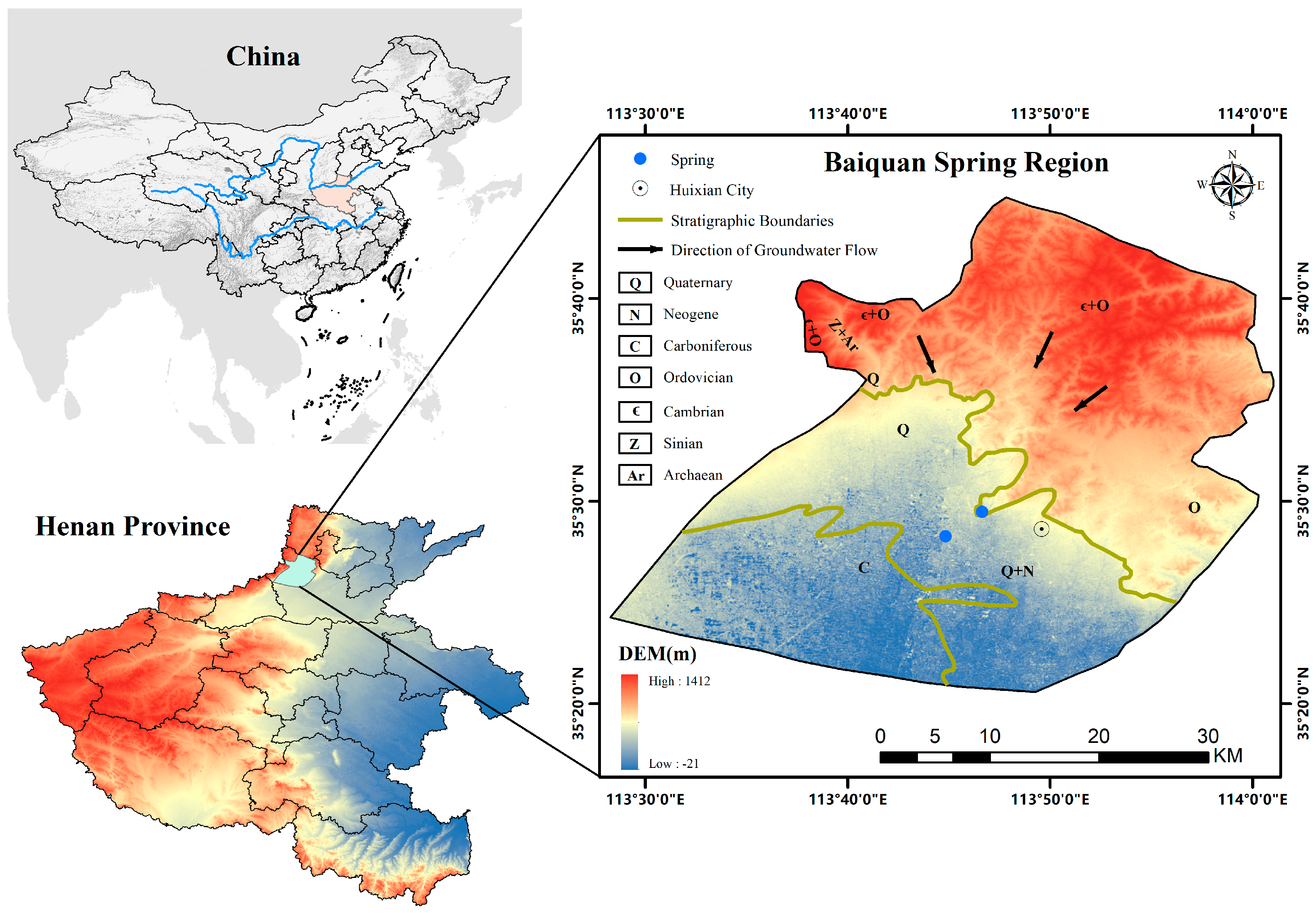
Figure 1. Baiquan Spring DEM.
Sustainability 17 08101 g001
Figure 2. Temperature Variation Distribution Ridge Plot.
Sustainability 17 08101 g002
Figure 3. FMD-mGTO-BiGRU-KAN model architecture diagram.
Sustainability 17 08101 g003
Figure 4. Architecture Diagram of Feature Mode Decomposition Model.
Sustainability 17 08101 g004
Figure 5. BiGRU model architecture diagram.
Sustainability 17 08101 g005
Figure 6. Evaluation of the predictive performance of the selective BiGRU-KAN hybrid model using varying numbers of decomposition components as input features. The numbers on the x - a x i s are arranged from small to large, where 0 means using the original undecomposed data. The number of decompositions starts from 3, and the maximum number is 15.
Sustainability 17 08101 g006
Figure 7. FMD decomposition mode and original data.
Sustainability 17 08101 g007
Figure 8. The global optimization trajectory of the mGTO algorithm is visualized, with the iteration count on the x - a x i s . The figure comprises four subplots: (a) illustrates the change in population size over the course of iterations, (b) shows the dynamic ratio of exploration to exploitation, (c) displays the evolution of fitness (global optimal value), and (d) presents the running time for each iteration.
Sustainability 17 08101 g008aSustainability 17 08101 g008b
Figure 9. Training and validation losses of FMD-mGTO-BiGRU-KAN (a), LSTM (b), GRU (c), and Transformer (d).
Sustainability 17 08101 g009
Figure 10. Evaluation indicators of the prediction effects of four models on different data sets.
Sustainability 17 08101 g010
Figure 11. Scatter plots of the predicted and observed discharges of Baiquan Spring during the four model prediction phases.
Sustainability 17 08101 g011
Figure 12. Violin plots of the predicted and observed Baiquan Spring discharge during the four model prediction stages.
Sustainability 17 08101 g012
Table 1. Model hyperparameter setting range during mGTO global optimization.
ParameterRange
look back3~30
learning rate5 × 10−5~1 × 10⁻³
num epochs200~600
batch size16~128
Table 2. The best results of hyperparameters for mGTO global optimization.
ParameterLook BackLearning RateNum EpochsBatch Size
result68.44306 × 10−430361
Table 3. Comparative analysis of calibration and validation performance among FMD-mGTO-BiGRU-KAN, LSTM, GRU, and Transformer.
FMD-mGTO-BiGRU-KANLSTMGRUTransformer
MSE-Train0.00140.00380.00440.0027
RMSE-Train0.03760.06180.06630.0515
NSE-Train0.96370.89540.87970.9274
MSE-Val0.00070.00390.00480.0038
RMSE-Val0.02600.06250.06930.0620
NSE-Val0.98350.92370.90630.9248
MSE-Pred0.07060.35150.48400.3734
RMSE-Pred0.26580.59290.69570.6111
NSE-Pred0.98250.92130.89160.9163
Disclaimer/Publisher’s Note: The statements, opinions and data contained in all publications are solely those of the individual author(s) and contributor(s) and not of MDPI and/or the editor(s). MDPI and/or the editor(s) disclaim responsibility for any injury to people or property resulting from any ideas, methods, instructions or products referred to in the content.